Dynamic Longevity Hedging in the Presence of …...Dynamic Longevity Hedging Residual Risk...

Dynamic Longevity Hedging Residual Risk Transferring

Dynamic Longevity Hedging in the Presence ofPopulation Basis Risk: A Feasibility Analysisfrom Technical and Economic Perspectives

Kenneth Q. Zhou and Johnny S.-H. Li

University of Waterloo

September 3, 2014

Kenneth Q. Zhou and Johnny S.-H. Li University of Waterloo

Dynamic Longevity Hedging


Outline

Figure 1: The outline of the proposed dynamic hedging strategy.




Overview

1 Dynamic Longevity HedgingConstructing the dynamic hedging strategyA two-population example

2 Residual Risk TransferringConstructing the customized surplus swapA multi-population example




Constructing the dynamic hedging strategy

Model and Approximation

The augmented common factor model (Li and Lee, 2005):

ln(m(i)x ,t) = a

(i)x + BxKt+1 + b

(i)x k

(i)t+1 + e

(i)x ,t , i = 1, 2, . . .

where

Kt follows a random walk:

Kt = c + Kt−1 + εt ;

k(i)t follows an AR(1) process:

k(i)t = c(i) + φ(i)k

(i)t−1 + ε

(i)t .





The approximation method - an extension of the work of Cairns(2011):

f(i)x ,t (T ,Kt , k

(i)t ) = Φ−1(p

(i)x ,t(T ,Kt , k

(i)t ))

≈ D(i)x ,t,0(T ) + D

(i)x ,t,1(T ) · (Kt − K̂t)

+ D(i)x ,t,2(T ) · (k

(i)t − k̂

(i)t )

where

Φ−1 is the probit function;

p(i)x,t(T ,Kt , k

(i)t ) is the time-t spot

survival probability for T years;

K̂t = E(Kt |K0);

k̂(i)t = E(k

(i)t |k

(i)0 );

D(i)x,t,0(T ) = f

(i)x,t (T , K̂t , k̂

(i)t );

D(i)x,t,1(T ) =

∂f(i)x,t (T ,Kt ,k̂

(i)t )

∂Kt

∣∣∣∣Kt=K̂t

;

D(i)x,t,2(T ) =

∂f(i)x,t (T ,K̂t ,k

(i)t )

∂k(i)t

∣∣∣∣k

(i)t =k̂

(i)t

.





Evaluation of the Required Quantities

To construct the dynamic hedging strategy, the followingquantities are calculated using the approximation method:

The time-t present value of the pension liabilities.

The time-t present value of the hedging instruments.

The first derivative with respect to Kt of the time-t presentvalue of the pension liabilities, ∆liab

Kt.

The first derivative with respect to Kt of the time-t presentvalue of the hedging instruments, ∆hedge

Kt.





Dynamic Hedging

To determine the optimal hedge ratio, ht , the first derivativesof the pension liabilities and the hedging instruments withrespect to Kt are matched:

∆liabKt

= ht · ∆hedgeKt

.

At time t, ht units of the hedging instruments are purchasedto hedge the uncertainty of the pension liabilities from time tto t + 1.

At time t + 1, the hedging instruments purchased at time tare closed out to compensate for the shortfall of the pensionplan from the longevity risk.





Hedge Effectiveness

The hedge effectiveness at time t is calculated as:

HEt = 1 − Var(Ht − Lt)

Var(Lt)

where

Lt is the time-0 present value of the realized liabilities fromtime 0 to t and the future liabilities after time t;

Ht is the time-0 present value of the payoffs of the hedginginstruments up to time t with an initial reserve of H0 = L0.




A two-population example

A Two-Population Example

Two populations: Continuous Mortality Investigation (CMI)and England and Wales (EW)

Liability: 30 years of $1 pension liabilities subject to themortality experience of a male individual aged 60 in year 2005from the CMI population.

Hedging instrument: 10-year age-75 q-forward contractslinked to the EW population, which are unlimitedly availableand liquidly traded.





0 5 10 15 20 25 30

14.3

14.4

14.5

14.6

14.7

14.8

14.9

15CMI: Liability

Time

L t

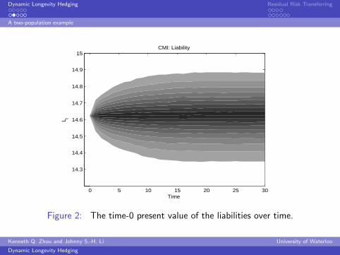
Figure 2: The time-0 present value of the liabilities over time.





0 5 10 15 20 250.015

0.02

0.025

0.03

0.035

0.04

Time

Rat

e

EW: q−forward

Figure 3: The 10-year age-75 q-forward rate over time.





0 5 10 15 20 25 300

20

40

60

80

100

120

140

160

Time

h t

No Population Basis Risk

0 5 10 15 20 25 300

20

40

60

80

100

120

140

160

Time

h t

Population Basis Risk

Figure 4: The optimal hedge ratio over time.





0 5 10 15 20 25 30−0.4

−0.3

−0.2

−0.1

0

0.1

0.2

0.3

0.4

Time

H t − L

t

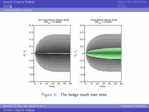
No Population Basis RiskHE30 = 0.9996

0 5 10 15 20 25 30−0.4

−0.3

−0.2

−0.1

0

0.1

0.2

0.3

0.4

Time

H t − L

t

Population Basis RiskHE30 = 0.9187

Figure 5: The hedge result over time.




Constructing the customized surplus swap

Motivations

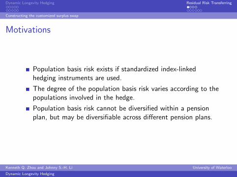
Population basis risk exists if standardized index-linkedhedging instruments are used.

The degree of the population basis risk varies according to thepopulations involved in the hedge.

Population basis risk cannot be diversified within a pensionplan, but may be diversifiable across different pension plans.





The Customized Surplus Swap

The swap is a cash exchange agreement between a pensionplan and a reinsurer.

It transfers population basis risk and sampling risk from oneparty to another.

The swap exchanges the economic surplus of a pension planafter the implementation of a dynamic longevity hedgingstrategy.

It eventually offloads the residual risk from the pension planto the counterparty.





The Surplus of a Pension Plan

The total liability of the pension plan at time t is

Lt = CLt + FLt ,

where CLt and FLt are the time-t values of the current andfuture liabilities, respectively.

The hedging portfolio for the pension plan at time t is

Ht = (1 + r)(Ht−1 − CLt−1) + Pt ,

where Pt is the payoff of the hedging instruments at time t,and H0 = L0 is the initial reserve.

Finally, the surplus of the pension plan at time t is defined as

SPt = Ht − Lt .





The Cash Flow of the Swap

The goal is to have SPt = 0. Hence, the cash flow of the swap attime t is defined as CFt = −SPt . It follows that

CFt = Lt − (1 + r)(Ht−1 − CLt−1) − Pt .

If the swap is set up every year, then

CFt = Lt − (1 + r)FLt−1 − Pt .

Both Lt and FLt−1 can be determined by whichever valuationmethods agreed to by the two parties. The payoff of the hedginginstruments will be determined by the market price at time t andthe number of holdings at time t − 1.




A multi-population example

A Multi-Population Example

20 national populations.

Liability: 30 years of $1 pension liabilities subject to themortality experience of a male individual aged 60 in year 2008from each population.

Hedging instrument: 10-year age-75 q-forward contractslinked to the EW population, which are unlimitedly availableand liquidly traded.

Sampling risk: a binomial frequency model with an assumedpopulation size of 10,000 for each population.





0 15 30−1

−0.5

0

0.5

1

Time

H t − L t

EWHE30=0.9668

0 15 30−1

−0.5

0

0.5

1

Time

H t − L t

SWEHE30=0.7247

0 15 30−1

−0.5

0

0.5

1

Time

H t − L t

FRAHE30=0.9054

0 15 30−1

−0.5

0

0.5

1

Time

H t − L t

BELHE30=0.9024

0 15 30−1

−0.5

0

0.5

1

Time

H t − L t

NLDHE30=0.68

0 15 30−1

−0.5

0

0.5

1

Time

H t − L t

CHEHE30=0.9289

0 15 30−1

−0.5

0

0.5

1

Time

H t − L t

CANHE30=0.853

0 15 30−1

−0.5

0

0.5

1

Time

H t − L t

NZLHE30=0.9479

0 15 30−1

−0.5

0

0.5

1

Time

H t − L t

PRTHE30=0.8504

0 15 30−1

−0.5

0

0.5

1

Time

H t − L t

ITAHE30=0.9511

0 15 30−1

−0.5

0

0.5

1

Time

H t − L t

NORHE30=0.6416

0 15 30−1

−0.5

0

0.5

1

Time

H t − L t

AUSHE30=0.7832

0 15 30−1

−0.5

0

0.5

1

Time

H t − L t

ESPHE30=0.7815

0 15 30−1

−0.5

0

0.5

1

Time

H t − L t

DEUWHE30=0.6855

0 15 30−1

−0.5

0

0.5

1

Time

H t − L t

AUTHE30=0.8528

0 15 30−1

−0.5

0

0.5

1

Time

H t − L t

USAHE30=0.7402

0 15 30−1

−0.5

0

0.5

1

Time

H t − L t

FINHE30=0.7053

0 15 30−1

−0.5

0

0.5

1

Time

H t − L t

LUXHE30=0.6467

0 15 30−1

−0.5

0

0.5

1

TimeH t −

L t

ISLHE30=0.5682

0 15 30−1

−0.5

0

0.5

1

Time

H t − L t

SCOHE30=0.4404

Figure 6: The hedge result over time for the 20 populations.





0 15 30−2

−1

0

1

2

Time

SPt

EW

0 15 30−2

−1

0

1

2

Time

SPt

SWE

0 15 30−2

−1

0

1

2

Time

SPt

FRA

0 15 30−2

−1

0

1

2

Time

SPt

BEL

0 15 30−2

−1

0

1

2

Time

SPt

NLD

0 15 30−2

−1

0

1

2

Time

SPt

CHE

0 15 30−2

−1

0

1

2

Time

SPt

CAN

0 15 30−2

−1

0

1

2

Time

SPt

NZL

0 15 30−2

−1

0

1

2

Time

SPt

PRT

0 15 30−2

−1

0

1

2

Time

SPt

ITA

0 15 30−2

−1

0

1

2

Time

SPt

NOR

0 15 30−2

−1

0

1

2

Time

SPt

AUS

0 15 30−2

−1

0

1

2

Time

SPt

ESP

0 15 30−2

−1

0

1

2

Time

SPt

DEUW

0 15 30−2

−1

0

1

2

Time

SPt

AUT

0 15 30−2

−1

0

1

2

Time

SPt

USA

0 15 30−2

−1

0

1

2

Time

SPt

FIN

0 15 30−2

−1

0

1

2

Time

SPt

LUX

0 15 30−2

−1

0

1

2

TimeSP

t

ISL

0 15 30−2

−1

0

1

2

Time

SPt

SCO

Figure 7: The surplus over time for the 20 populations.





0 15 30−0.2

−0.1

0

0.1

0.2

Time

CFt

EW

0 15 30−0.2

−0.1

0

0.1

0.2

Time

CFt

SWE

0 15 30−0.2

−0.1

0

0.1

0.2

Time

CFt

FRA

0 15 30−0.2

−0.1

0

0.1

0.2

Time

CFt

BEL

0 15 30−0.2

−0.1

0

0.1

0.2

Time

CFt

NLD

0 15 30−0.2

−0.1

0

0.1

0.2

Time

CFt

CHE

0 15 30−0.2

−0.1

0

0.1

0.2

Time

CFt

CAN

0 15 30−0.2

−0.1

0

0.1

0.2

Time

CFt

NZL

0 15 30−0.2

−0.1

0

0.1

0.2

Time

CFt

PRT

0 15 30−0.2

−0.1

0

0.1

0.2

Time

CFt

ITA

0 15 30−0.2

−0.1

0

0.1

0.2

Time

CFt

NOR

0 15 30−0.2

−0.1

0

0.1

0.2

Time

CFt

AUS

0 15 30−0.2

−0.1

0

0.1

0.2

TimeCF

t

ESP

0 15 30−0.2

−0.1

0

0.1

0.2

Time

CFt

DEUW

0 15 30−0.2

−0.1

0

0.1

0.2

Time

CFt

AUT

0 15 30−0.2

−0.1

0

0.1

0.2

Time

CFt

USA

0 15 30−0.2

−0.1

0

0.1

0.2

Time

CFt

FIN

0 15 30−0.2

−0.1

0

0.1

0.2

Time

CFt

LUX

0 15 30−0.2

−0.1

0

0.1

0.2

Time

CFt

ISL

0 15 30−0.2

−0.1

0

0.1

0.2

Time

CFt

SCO

Figure 8: The cash flow over time for the 20 populations.





0 5 10 15 20 25 30−0.2

−0.15

−0.1

−0.05

0

0.05

0.1

0.15

0.2Mean Cash Flow

Time

CF t

Figure 9: The mean cash flow of the 20 populations.





Conclusion

Figure 10: The outline of the proposed dynamic hedging strategy.



Dynamic Longevity Hedging in the Presence of …...Dynamic Longevity Hedging Residual Risk...

Documents

Transcript of Dynamic Longevity Hedging in the Presence of …...Dynamic Longevity Hedging Residual Risk...