Trading to hedge: dynamic hedging - New York Universitypeople.stern.nyu.edu/jhasbrou/Teaching/POST...
18
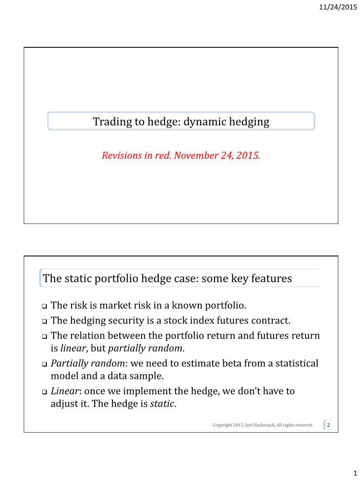
1 11/24/2015 Trading to hedge: dynamic hedging Revisions in red. November 24, 2015. The static portfolio hedge case: some key features The risk is market risk in a known portfolio. The hedging security is a stock index futures contract. The relation between the portfolio return and futures return is linear, but partially random. Partially random: we need to estimate beta from a statistical model and a data sample. Linear: once we implement the hedge, we don’t have to adjust it. The hedge is static. Copyright 2015, Joel Hasbrouck, All rights reserved 2
Transcript of Trading to hedge: dynamic hedging - New York Universitypeople.stern.nyu.edu/jhasbrou/Teaching/POST...
1
11/24/2015
Trading to hedge: dynamic hedging
Revisions in red. November 24, 2015.
The static portfolio hedge case: some key features
The risk is market risk in a known portfolio.
The hedging security is a stock index futures contract.
The relation between the portfolio return and futures return is linear, but partially random.
Partially random: we need to estimate beta from a statistical model and a data sample.
Linear: once we implement the hedge, we don’t have to adjust it. The hedge is static.
Copyright 2015, Joel Hasbrouck, All rights reserved 2
2
11/24/2015
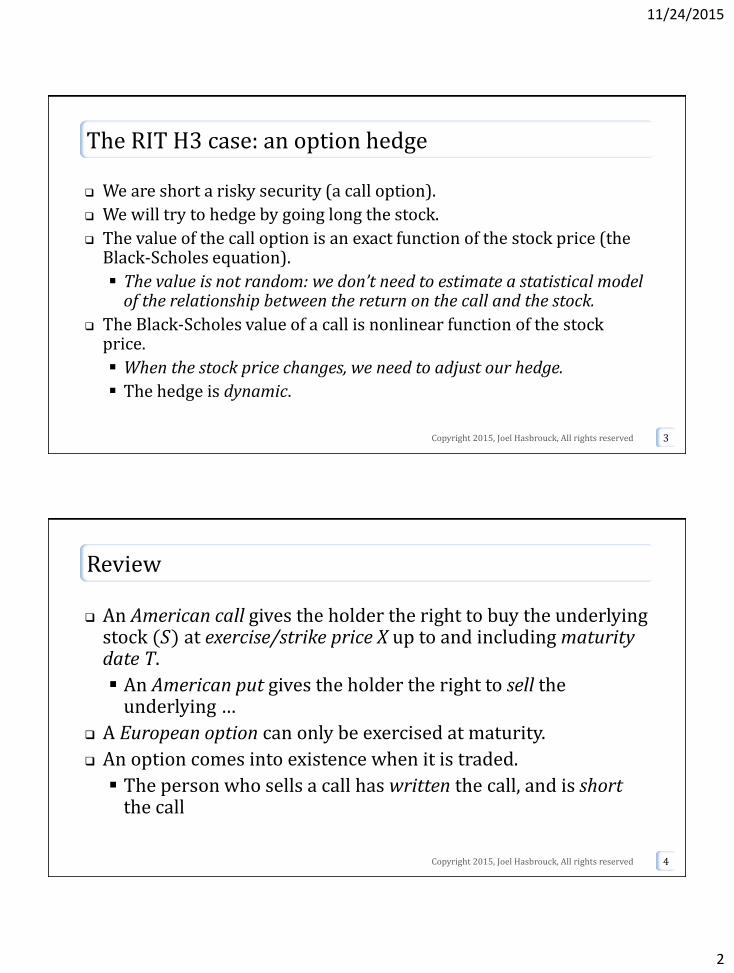
The RIT H3 case: an option hedge
We are short a risky security (a call option).
We will try to hedge by going long the stock.
The value of the call option is an exact function of the stock price (the Black-Scholes equation).
The value is not random: we don’t need to estimate a statistical model of the relationship between the return on the call and the stock.
The Black-Scholes value of a call is nonlinear function of the stock price.
When the stock price changes, we need to adjust our hedge.
The hedge is dynamic.
Copyright 2015, Joel Hasbrouck, All rights reserved 3
Review
An American call gives the holder the right to buy the underlying stock (𝑆) at exercise/strike price X up to and including maturity date T.
An American put gives the holder the right to sell the underlying …
A European option can only be exercised at maturity.
An option comes into existence when it is traded.
The person who sells a call has written the call, and is shortthe call
Copyright 2015, Joel Hasbrouck, All rights reserved 4
3
11/24/2015
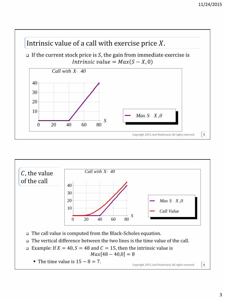
Intrinsic value of a call with exercise price 𝑋.
If the current stock price is 𝑆, the gain from immediate exercise is𝐼𝑛𝑡𝑟𝑖𝑛𝑠𝑖𝑐 𝑣𝑎𝑙𝑢𝑒 = 𝑀𝑎𝑥 𝑆 − 𝑋, 0
Copyright 2015, Joel Hasbrouck, All rights reserved 5
0 20 40 60 80S
10
20
30
40
Call with X 40
Max S X ,0
𝐶, the value of the call
The call value is computed from the Black-Scholes equation.
The vertical difference between the two lines is the time value of the call.
Example: If 𝑋 = 40, 𝑆 = 48 and 𝐶 = 15, then the intrinsic value is𝑀𝑎𝑥 48 − 40,0 = 8
The time value is 15 − 8 = 7.6
0 20 40 60 80S
10
20
30
40
Call with X 40
Call Value
Max S X ,0
Copyright 2015, Joel Hasbrouck, All rights reserved
4
11/24/2015
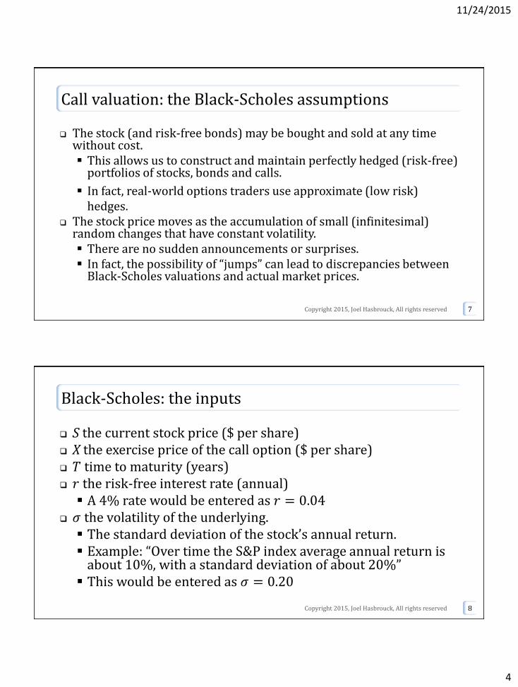
Call valuation: the Black-Scholes assumptions
The stock (and risk-free bonds) may be bought and sold at any time without cost. This allows us to construct and maintain perfectly hedged (risk-free)
portfolios of stocks, bonds and calls.
In fact, real-world options traders use approximate (low risk) hedges.
The stock price moves as the accumulation of small (infinitesimal) random changes that have constant volatility. There are no sudden announcements or surprises. In fact, the possibility of “jumps” can lead to discrepancies between
Black-Scholes valuations and actual market prices.
Copyright 2015, Joel Hasbrouck, All rights reserved 7
Black-Scholes: the inputs
S the current stock price ($ per share) X the exercise price of the call option ($ per share) 𝑇 time to maturity (years) 𝑟 the risk-free interest rate (annual) A 4% rate would be entered as 𝑟 = 0.04
𝜎 the volatility of the underlying. The standard deviation of the stock’s annual return. Example: “Over time the S&P index average annual return is
about 10%, with a standard deviation of about 20%” This would be entered as 𝜎 = 0.20
Copyright 2015, Joel Hasbrouck, All rights reserved 8
5
11/24/2015
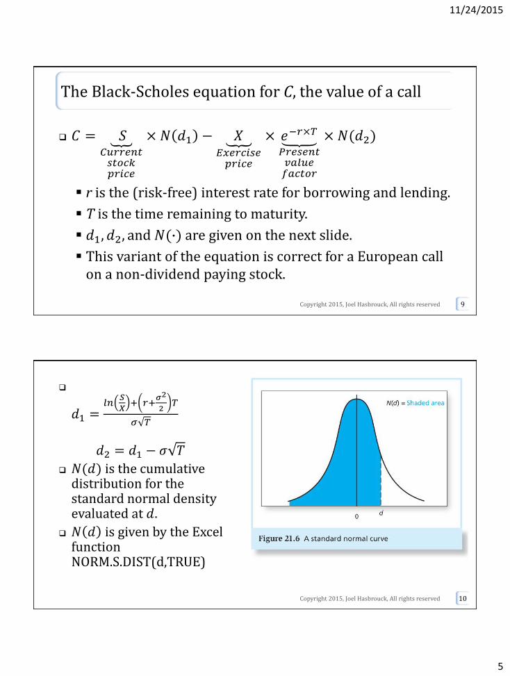
The Black-Scholes equation for C, the value of a call
𝐶 = 𝑆𝐶𝑢𝑟𝑟𝑒𝑛𝑡𝑠𝑡𝑜𝑐𝑘𝑝𝑟𝑖𝑐𝑒
× 𝑁 𝑑1 − 𝑋𝐸𝑥𝑒𝑟𝑐𝑖𝑠𝑒𝑝𝑟𝑖𝑐𝑒
× 𝑒−𝑟×𝑇
𝑃𝑟𝑒𝑠𝑒𝑛𝑡𝑣𝑎𝑙𝑢𝑒𝑓𝑎𝑐𝑡𝑜𝑟
× 𝑁(𝑑2)
r is the (risk-free) interest rate for borrowing and lending.
T is the time remaining to maturity.
𝑑1, 𝑑2, and 𝑁(∙) are given on the next slide.
This variant of the equation is correct for a European call on a non-dividend paying stock.
Copyright 2015, Joel Hasbrouck, All rights reserved 9
𝑑1 =𝑙𝑛𝑆
𝑋+ 𝑟+𝜎2
2𝑇
𝜎 𝑇
𝑑2 = 𝑑1 − 𝜎 𝑇
𝑁(𝑑) is the cumulative distribution for the standard normal density evaluated at 𝑑.
𝑁 𝑑 is given by the Excel function NORM.S.DIST(d,TRUE)
10Copyright 2015, Joel Hasbrouck, All rights reserved
6
11/24/2015
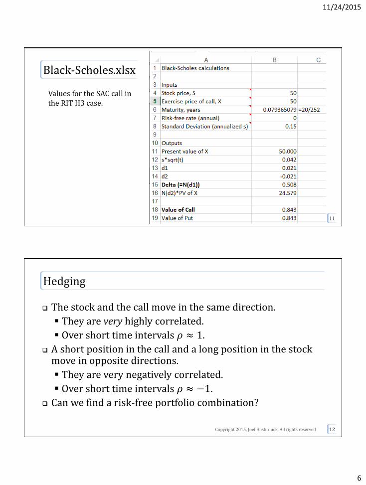
Black-Scholes.xlsx
Copyright 2015, Joel Hasbrouck, All rights reserved 11
Values for the SAC call in the RIT H3 case.
Hedging
The stock and the call move in the same direction.
They are very highly correlated.
Over short time intervals 𝜌 ≈ 1.
A short position in the call and a long position in the stock move in opposite directions.
They are very negatively correlated.
Over short time intervals 𝜌 ≈ −1.
Can we find a risk-free portfolio combination?
Copyright 2015, Joel Hasbrouck, All rights reserved 12
7
11/24/2015
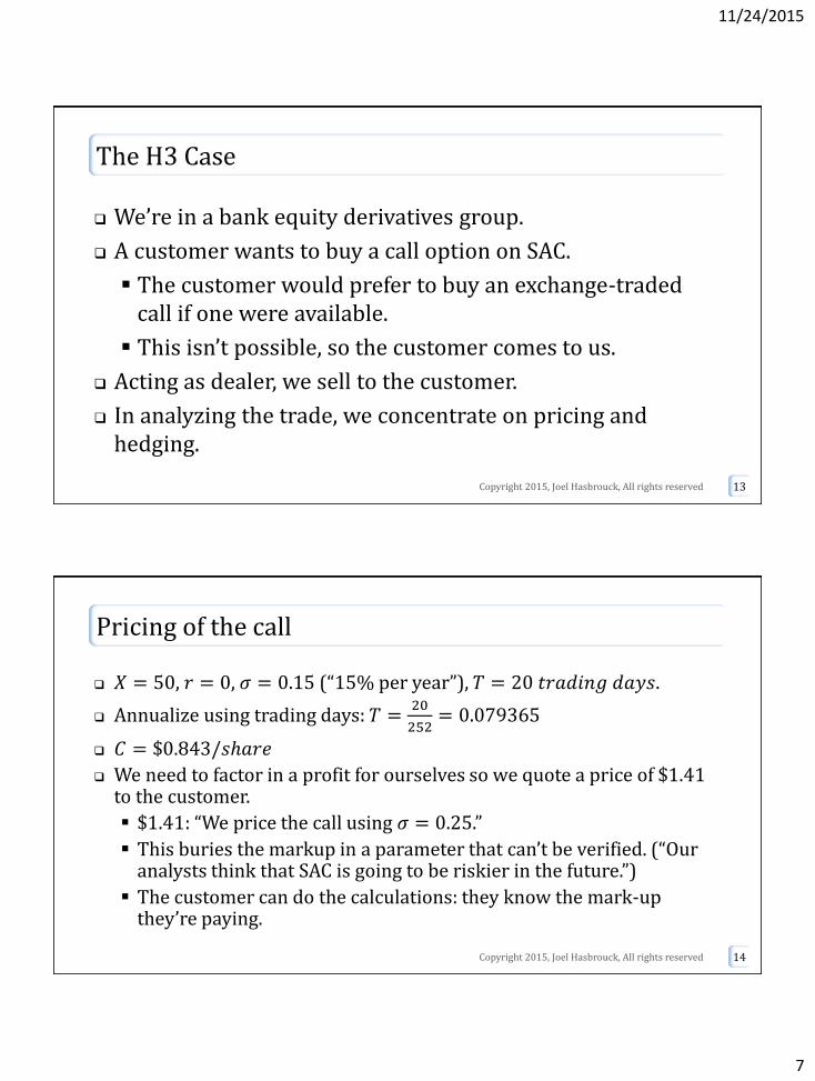
The H3 Case
We’re in a bank equity derivatives group.
A customer wants to buy a call option on SAC.
The customer would prefer to buy an exchange-traded call if one were available.
This isn’t possible, so the customer comes to us.
Acting as dealer, we sell to the customer.
In analyzing the trade, we concentrate on pricing and hedging.
Copyright 2015, Joel Hasbrouck, All rights reserved 13
Pricing of the call
𝑋 = 50, 𝑟 = 0, 𝜎 = 0.15 (“15% per year”), 𝑇 = 20 𝑡𝑟𝑎𝑑𝑖𝑛𝑔 𝑑𝑎𝑦𝑠.
Annualize using trading days: 𝑇 =20
252= 0.079365
𝐶 = $0.843/𝑠ℎ𝑎𝑟𝑒
We need to factor in a profit for ourselves so we quote a price of $1.41 to the customer.
$1.41: “We price the call using 𝜎 = 0.25.”
This buries the markup in a parameter that can’t be verified. (“Our analysts think that SAC is going to be riskier in the future.”)
The customer can do the calculations: they know the mark-up they’re paying.
Copyright 2015, Joel Hasbrouck, All rights reserved 14
8
11/24/2015
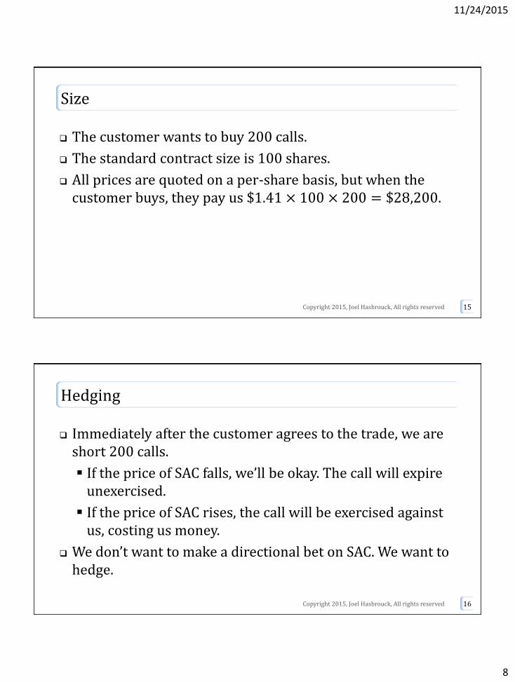
Size
The customer wants to buy 200 calls.
The standard contract size is 100 shares.
All prices are quoted on a per-share basis, but when the customer buys, they pay us $1.41 × 100 × 200 = $28,200.
Copyright 2015, Joel Hasbrouck, All rights reserved 15
Hedging
Immediately after the customer agrees to the trade, we are short 200 calls.
If the price of SAC falls, we’ll be okay. The call will expire unexercised.
If the price of SAC rises, the call will be exercised against us, costing us money.
We don’t want to make a directional bet on SAC. We want to hedge.
Copyright 2015, Joel Hasbrouck, All rights reserved 16
9
11/24/2015
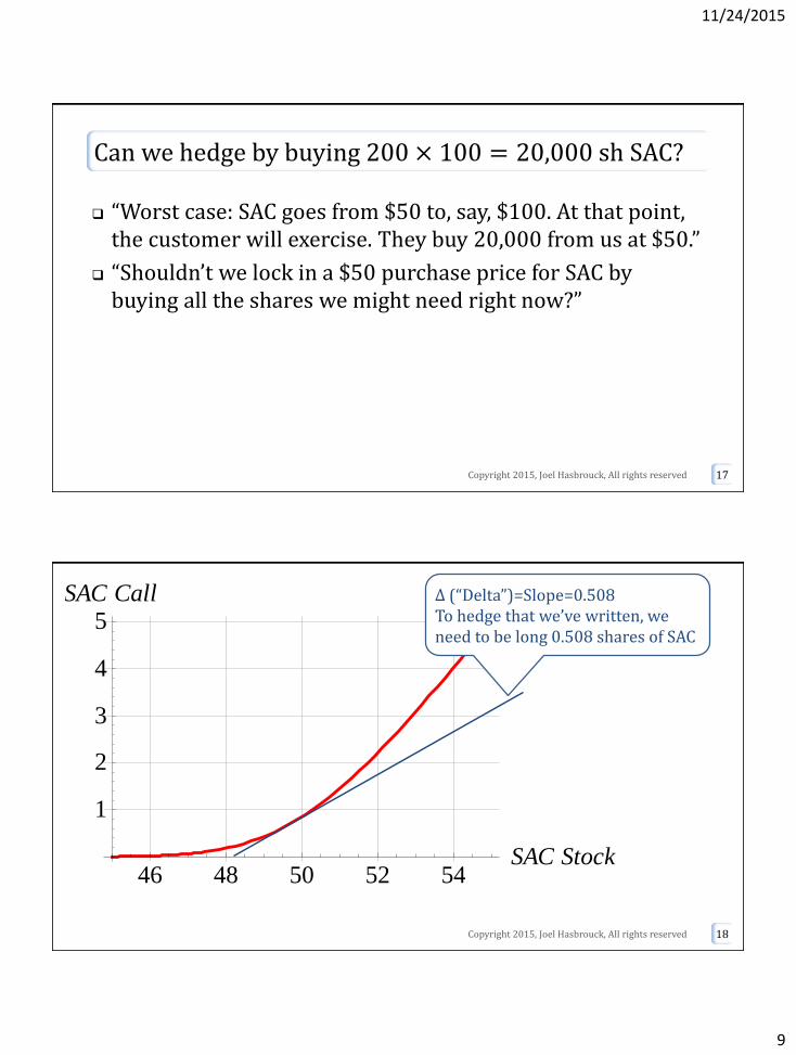
Can we hedge by buying 200 × 100 = 20,000 sh SAC?
“Worst case: SAC goes from $50 to, say, $100. At that point, the customer will exercise. They buy 20,000 from us at $50.”
“Shouldn’t we lock in a $50 purchase price for SAC by buying all the shares we might need right now?”
Copyright 2015, Joel Hasbrouck, All rights reserved 17
Copyright 2015, Joel Hasbrouck, All rights reserved 18
46 48 50 52 54SAC Stock
1
2
3
4
5SAC Call Δ (“Delta”)=Slope=0.508
To hedge that we’ve written, we need to be long 0.508 shares of SAC
10
11/24/2015
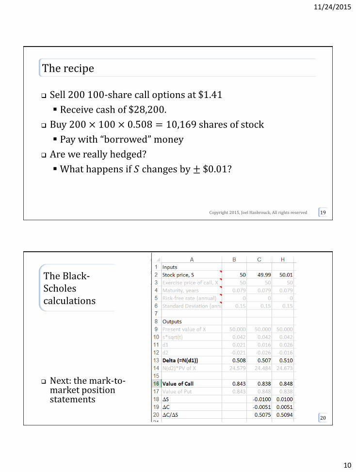
The recipe
Sell 200 100-share call options at $1.41
Receive cash of $28,200.
Buy 200 × 100 × 0.508 = 10,169 shares of stock
Pay with “borrowed” money
Are we really hedged?
What happens if 𝑆 changes by ± $0.01?
Copyright 2015, Joel Hasbrouck, All rights reserved 19
The Black-Scholes calculations
Next: the mark-to-market position statements
20
11
11/24/2015
21
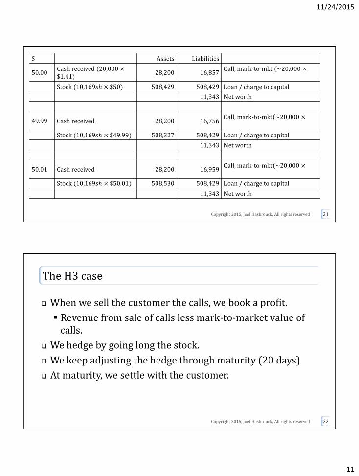
S Assets Liabilities
50.00Cash received (20,000 ×$1.41)
28,200 16,857Call, mark-to-mkt (~20,000 ×
Stock (10,169𝑠ℎ × $50) 508,429 508,429 Loan / charge to capital
11,343 Net worth
49.99 Cash received 28,200 16,756Call, mark-to-mkt(~20,000 ×
Stock (10,169𝑠ℎ × $49.99) 508,327 508,429 Loan / charge to capital
11,343 Net worth
50.01 Cash received 28,200 16,959Call, mark-to-mkt(~20,000 ×
Stock (10,169𝑠ℎ × $50.01) 508,530 508,429 Loan / charge to capital
11,343 Net worth
Copyright 2015, Joel Hasbrouck, All rights reserved
The H3 case
When we sell the customer the calls, we book a profit.
Revenue from sale of calls less mark-to-market value of calls.
We hedge by going long the stock.
We keep adjusting the hedge through maturity (20 days)
At maturity, we settle with the customer.
Copyright 2015, Joel Hasbrouck, All rights reserved 22
12
11/24/2015
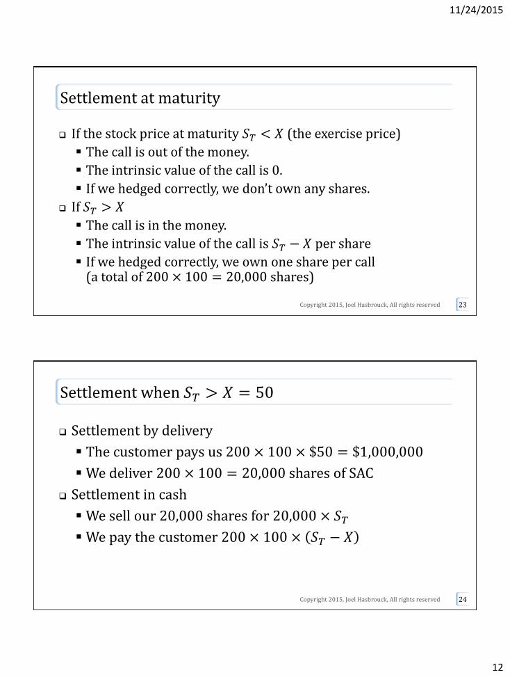
Settlement at maturity
If the stock price at maturity 𝑆𝑇 < 𝑋 (the exercise price)
The call is out of the money.
The intrinsic value of the call is 0.
If we hedged correctly, we don’t own any shares.
If 𝑆𝑇 > 𝑋
The call is in the money.
The intrinsic value of the call is 𝑆𝑇 − 𝑋 per share
If we hedged correctly, we own one share per call (a total of 200 × 100 = 20,000 shares)
Copyright 2015, Joel Hasbrouck, All rights reserved 23
Settlement when 𝑆𝑇 > 𝑋 = 50
Settlement by delivery
The customer pays us 200 × 100 × $50 = $1,000,000
We deliver 200 × 100 = 20,000 shares of SAC
Settlement in cash
We sell our 20,000 shares for 20,000 × 𝑆𝑇 We pay the customer 200 × 100 × 𝑆𝑇 − 𝑋
Copyright 2015, Joel Hasbrouck, All rights reserved 24
13
11/24/2015
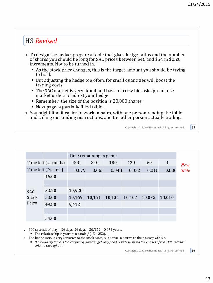
H3 Revised
To design the hedge, prepare a table that gives hedge ratios and the number of shares you should be long for SAC prices between $46 and $54 in $0.20 increments. Not to be turned in. As the stock price changes, this is the target amount you should be trying
to hold. But adjusting the hedge too often, for small quantities will boost the
trading costs. The SAC market is very liquid and has a narrow bid-ask spread: use
market orders to adjust your hedge. Remember: the size of the position is 20,000 shares. Next page: a partially filled table …
You might find it easier to work in pairs, with one person reading the table and calling out trading instructions, and the other person actually trading.
Copyright 2015, Joel Hasbrouck, All rights reserved 25
300 seconds of play = 20 days; 20 days = 20/252 = 0.079 years. The relationship is years = seconds / (15 x 252).
The hedge ratio is very sensitive to the stock price, but not so sensitive to the passage of time. If a two-way table is too confusing, you can get very good results by using the entries of the “300 second”
column throughout.
Copyright 2015, Joel Hasbrouck, All rights reserved 26
Time remaining in game
Time left (seconds) 300 240 180 120 60 1
Time left (“years”) 0.079 0.063 0.048 0.032 0.016 0.000
SACStockPrice
46.00
…
50.20 10,920
50.00 10,169 10,151 10,131 10,107 10,075 10,010
49.80 9,412
…
54.00
New Slide
14
11/24/2015
Practical complications
We’ve concentrated on hedging short term changes in the stock price S.
This is called delta hedging.
The hedge ratio also depends on 𝑇, 𝑟 and 𝜎.
𝜎 depends on market conditions and new information.
Even if 𝑟 and 𝜎 are constant, T will change with the passage of time.
Copyright 2015, Joel Hasbrouck, All rights reserved 27
Adjusting the hedge requires us to trade in the direction of the market.
We sell when S falls, buy when S rises.
Do our trades push the price against us?
Are there other traders who are also trying to delta-hedge?
What if there is a significant news announcement when the market is closed?
Copyright 2015, Joel Hasbrouck, All rights reserved 28
15
11/24/2015
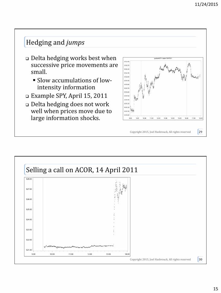
Hedging and jumps
Delta hedging works best when successive price movements are small.
Slow accumulations of low-intensity information
Example SPY, April 15, 2011
Delta hedging does not work well when prices move due to large information shocks.
Copyright 2015, Joel Hasbrouck, All rights reserved 29
Selling a call on ACOR, 14 April 2011
Copyright 2015, Joel Hasbrouck, All rights reserved 30
16
11/24/2015
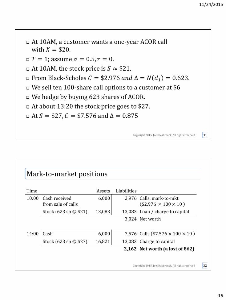
At 10AM, a customer wants a one-year ACOR call with 𝑋 = $20.
𝑇 = 1; assume 𝜎 = 0.5, 𝑟 = 0.
At 10AM, the stock price is 𝑆 ≈ $21.
From Black-Scholes 𝐶 = $2.976 𝑎𝑛𝑑 Δ = 𝑁 𝑑1 = 0.623.
We sell ten 100-share call options to a customer at $6
We hedge by buying 623 shares of ACOR.
At about 13:20 the stock price goes to $27.
At 𝑆 = $27, 𝐶 = $7.576 and Δ = 0.875
Copyright 2015, Joel Hasbrouck, All rights reserved 31
Mark-to-market positions
Copyright 2015, Joel Hasbrouck, All rights reserved 32
Time Assets Liabilities
10:00 Cash receivedfrom sale of calls
6,000 2,976 Calls, mark-to-mkt $2.976 × 100 × 10
Stock (623 sh @ $21) 13,083 13,083 Loan / charge to capital
3,024 Net worth
14:00 Cash 6,000 7,576 Calls $7.576 × 100 × 10
Stock (623 sh @ $27) 16,821 13,083 Charge to capital
2,162 Net worth (a lost of 862)
17
11/24/2015
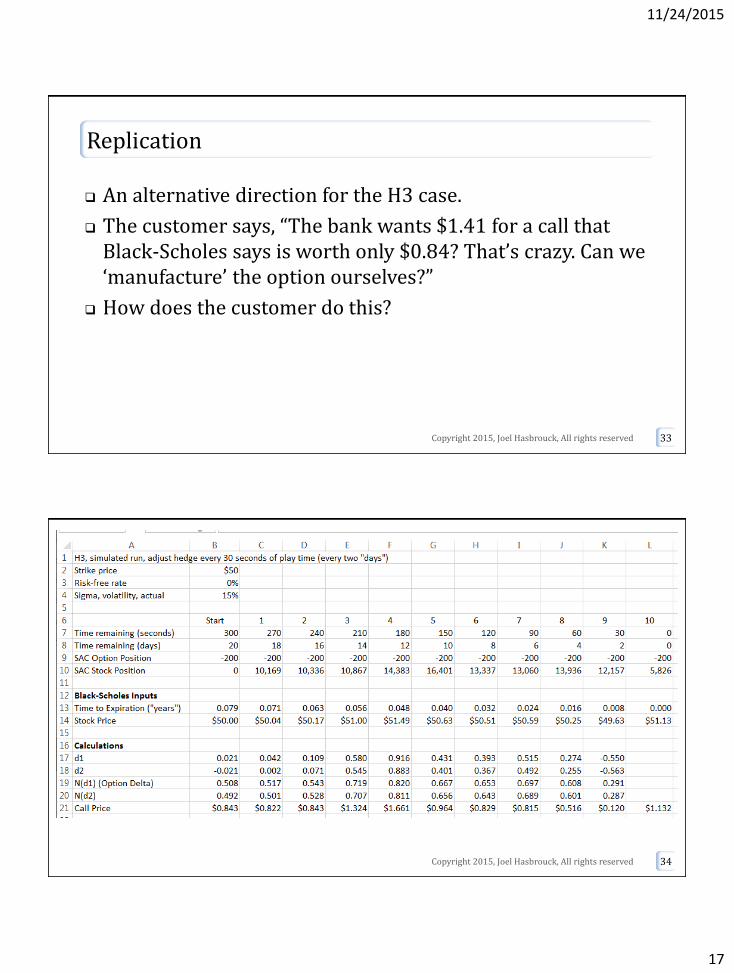
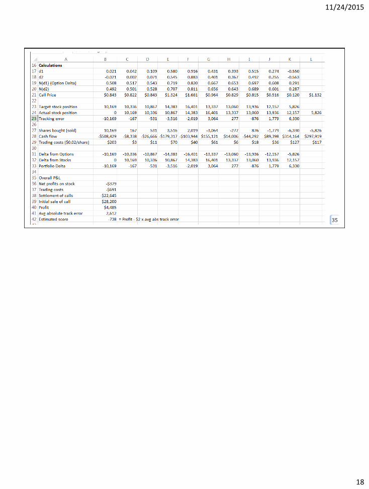
Replication
An alternative direction for the H3 case.
The customer says, “The bank wants $1.41 for a call that Black-Scholes says is worth only $0.84? That’s crazy. Can we ‘manufacture’ the option ourselves?”
How does the customer do this?
Copyright 2015, Joel Hasbrouck, All rights reserved 33
Copyright 2015, Joel Hasbrouck, All rights reserved 34
18
11/24/2015
Copyright 2015, Joel Hasbrouck, All rights reserved 35