
DSGE Model-Based Forecasting · DSGE Model-Based Forecasting S FRBNY f. ... theory to explain and...
95
This paper presents preliminary findings and is being distributed to economists and other interested readers solely to stimulate discussion and elicit comments. The views expressed in this paper are those of the authors and are not necessarily reflective of views at the Federal Reserve Bank of New York or the Federal Reserve System. Any errors or omissions are the responsibility of the authors. Federal Reserve Bank of New York Staff Reports Staff Report No. 554 March 2012 Marco Del Negro Frank Schorfheide DSGE Model-Based Forecasting REPORTS FRBNY Staff
Transcript of DSGE Model-Based Forecasting · DSGE Model-Based Forecasting S FRBNY f. ... theory to explain and...

This paper presents preliminary fi ndings and is being distributed to economists and other interested readers solely to stimulate discussion and elicit comments. The views expressed in this paper are those of the authors and are not necessarily refl ective of views at the Federal Reserve Bank of New York or the Federal Reserve System. Any errors or omissions are the responsibility of the authors.
Federal Reserve Bank of New YorkStaff Reports
Staff Report No. 554March 2012
Marco Del NegroFrank Schorfheide
DSGE Model-Based Forecasting
REPORTS
FRBNY
Staff
Del Negro: Federal Reserve Bank of New York (e-mail: [email protected]). Schorfheide: University of Pennsylvania (e-mail: [email protected]). Schorfheide gratefully acknowledges fi nancial support from the National Science Foundation under Grant SES 1061358. The completion of this project owes much to the outstanding research assistance of Minchul Shin and especially Daniel Herbst. For helpful comments and suggestions, the authors thank Keith Sill, as well as seminar participants at the 2012 American Economic Association meetings, the 2011 Asian meetings of the Econometric Society, the 2011 Canon Institute for Global Studies Conference on Macroeconomic Theory and Policy, the National Bank of Poland conference “DSGE Models and Beyond,” and Norges Bank. They also thank Rochelle Edge and Refet Gürkaynak for providing and explaining the real-time data and Stefano Eusepi and Emanuel Möench for furnishing the survey data. The views expressed in this paper are those of the authors and do not necessarily refl ect the position of the Federal Reserve Bank of New York or the Federal Reserve System.
Abstract
Dynamic stochastic general equilibrium (DSGE) models use modern macroeconomic theory to explain and predict comovements of aggregate time series over the business cycle and to perform policy analysis. We explain how to use DSGE models for all three purposes―forecasting, story telling, and policy experiments―and review their forecast-ing record. We also provide our own real-time assessment of the forecasting performance of the Smets and Wouters (2007) model data up to 2011, compare it with Blue Chip and Greenbook forecasts, and show how it changes as we augment the standard set of ob-servables with external information from surveys (nowcasts, interest rate forecasts, and expectations for long-run infl ation and output growth). We explore methods of generat-ing forecasts in the presence of a zero-lower-bound constraint on nominal interest rates and conditional on counterfactual interest rate paths. Finally, we perform a postmortem of DSGE model forecasts of the Great Recession and show that forecasts from a version of the Smets-Wouters model augmented by fi nancial frictions, and using spreads as an observable, compare well with Blue Chip forecasts.
Key words: DSGE models, forecasting
DSGE Model-Based ForecastingMarco Del Negro and Frank SchorfheideFederal Reserve Bank of New York Staff Reports, no. 554March 2012JEL classifi cation: C11, C52, C54
Contents
1 Introduction 1
2 The DSGE Models 3
2.1 The Smets-Wouters Model . . . . . . . . . . . . . . . . . . . . . . . . . . . . 4
2.2 A Medium-Scale Model with Financial Frictions . . . . . . . . . . . . . . . . 8
2.3 A Small-Scale DSGE Model . . . . . . . . . . . . . . . . . . . . . . . . . . . 8
3 Generating Forecasts with DSGE Models 11
3.1 Posterior Inference for θ . . . . . . . . . . . . . . . . . . . . . . . . . . . . . 12
3.2 Evaluating the Predictive Distribution . . . . . . . . . . . . . . . . . . . . . 15
4 Accuracy of Point Forecasts 17
4.1 A Real Time Data Set for Forecast Evaluation . . . . . . . . . . . . . . . . . 17
4.2 Forecasts from the Small-Scale Model . . . . . . . . . . . . . . . . . . . . . . 21
4.3 Forecasts from the Smets-Wouters Model . . . . . . . . . . . . . . . . . . . . 22
4.4 Literature Review of Forecasting Performance . . . . . . . . . . . . . . . . . 26
5 DSGE Model Forecasts using External Information 32
5.1 Incorporating Long-Run Inflation Expectations . . . . . . . . . . . . . . . . 33
5.2 Incorporating Output Expectations . . . . . . . . . . . . . . . . . . . . . . . 36
5.3 Conditioning on External Nowcasts . . . . . . . . . . . . . . . . . . . . . . . 39
5.4 Incorporating Interest Rate Expectations . . . . . . . . . . . . . . . . . . . . 46
6 Forecasts Conditional on Interest Rate Paths 51
6.1 The Effects of Monetary Policy Shocks . . . . . . . . . . . . . . . . . . . . . 52
6.2 Using Unanticipated Shocks to Condition on Interest Rates . . . . . . . . . . 56
6.3 Using Anticipated Shocks to Condition on Interest Rates . . . . . . . . . . . 58
6.4 Forecasting Conditional on an Interest Rate Path: An Empirical Illustration 62

7 Moving Beyond Point Forecasts 63
7.1 Shock Decompositions . . . . . . . . . . . . . . . . . . . . . . . . . . . . . . 64
7.2 Real-Time DSGE Density Forecasts During the Great Recession: A Post-
Mortem . . . . . . . . . . . . . . . . . . . . . . . . . . . . . . . . . . . . . . 67
7.3 Calibration of Density Forecasts . . . . . . . . . . . . . . . . . . . . . . . . . 73
8 Conclusion and Outlook 77
8.1 Why DSGE Model Forecasting? . . . . . . . . . . . . . . . . . . . . . . . . . 77
8.2 Beyond DSGE Models . . . . . . . . . . . . . . . . . . . . . . . . . . . . . . 79
8.3 The Future . . . . . . . . . . . . . . . . . . . . . . . . . . . . . . . . . . . . 81
A Details for Figure 4 A-1

Del Negro, Schorfheide – DSGE Model Based Forecasting: February 29, 2012 1
1 Introduction
[sec:intro] Dynamic stochastic general equilibrium (DSGE) models use modern macroeco-
nomic theory to explain and predict comovements of aggregate time series over the business
cycle. The term DSGE model encompasses a broad class of macroeconomic models that spans
the standard neoclassical growth model discussed in King, Plosser, and Rebelo (1988) as well
as New Keynesian monetary models with numerous real and nominal frictions that are based
on the work of Christiano, Eichenbaum, and Evans (2005) and Smets and Wouters (2003).
A common feature of these models is that decision rules of economic agents are derived from
assumptions about preferences, technologies, and the prevailing fiscal and monetary policy
regime by solving intertemporal optimization problems. As a consequence, the DSGE model
paradigm delivers empirical models with a strong degree of theoretical coherence that are
attractive as a laboratory for policy experiments.
DSGE models are increasingly being used by central banks around the world as tools for
macroeconomic forecasting and policy analysis. Examples of such models include the small
open economy model developed by the Sveriges Riksbank (Adolfson, Linde, and Villani
(2007) and Adolfson, Andersson, Linde, Villani, and Vredin (2007)), the New Area-Wide
Model developed at the European Central Bank (Coenen, McAdam, and Straub (2008) and
Christoffel, Coenen, and Warne (2010)), and the Federal Reserve Board’s new Estimated,
Dynamic, Optimization-based model (Edge, Kiley, and Laforte (2009)). DSGE models are
frequently estimated with Bayesian methods (see, for instance, An and Schorfheide (2007a)
or Del Negro and Schorfheide (2010) for a review), in particular if the goal is to track
and forecast macroeconomic time series. Bayesian inference delivers posterior predictive
distributions that reflect uncertainty about latent state variables, parameters, and future
realizations of shocks conditional on the available information.
The contribution of this paper has a methodological and a substantive dimension. On
the methodological side, we provide a collection of algorithms that can be used to generate
forecasts with DSGE models that have been estimated with Bayesian methods. In particular,
we focus on novel methods that allow the user to incorporate external information into the
DSGE-model-based forecasts. This external information could take the form of forecasts
for the current quarter (nowcasts) from surveys of professional forecasters, short-term and
medium-term interest rate forecasts, or long-run inflation and output-growth expectations.

Del Negro, Schorfheide – DSGE Model Based Forecasting: February 29, 2012 2
We also study the use of unanticipated and anticipated monetary policy shocks to generate
forecasts conditional on desired interest rate paths.
On the substantive side, we are providing detailed empirical applications of the fore-
casting methods. The empirical analysis features small and medium-scale DSGE models
estimated on U.S. data. The novel aspects of the empirical analysis are to document how
the forecast performance of the Smets and Wouters (2007) model can be improved by in-
corporating data on long-run inflation expectations as well as nowcasts from the Blue Chip
survey. We also show that data on short- and medium-horizon interest rate expectations
improves the interest rate forecasts of the Smets-Wouters model with anticipated monetary
policy shocks, but has some adverse effects on output growth and inflation forecasts. Fi-
nally, we provide new insights in the real-time forecasting performance of the Smets-Wouters
model and a DSGE model with financial frictions during the 2008-09 recession.
The remainder of this paper is organized as follows. Section 2 provides a description of
the DSGE models used in the empirical analysis of this paper. The mechanics of generating
DSGE model forecasts within a Bayesian framework are described in Section 3. We review
well-known procedures to generate draws from posterior parameter distributions and poste-
rior predictive distributions for future realizations of macroeconomic variables. From these
draws one can then compute point, interval, and density forecasts. The first set of empirical
results is presented in Section 4. We describe the real-time data set that is used throughout
this paper and examine the accuracy of our benchmark point forecasts. We also provide a
review of the sizeable literature on the accuracy of DSGE model forecasts.
The accuracy of DSGE model forecasts is affected by how well the model captures low
frequency trends in the data and the extent to which important information about the current
quarter (nowcast) is incorporated into the forecast. In Section 5 we introduce shocks to the
target-inflation rate, long-run productivity growth, as well as anticipated monetary policy
shocks into the Smets and Wouters (2007) model. With these additional shocks, we can use
data on inflation, output growth, and interest rate expectations from the Blue Chip survey
as observations on agents’ expectations in the DSGE model and thereby incorporate the
survey information into the DSGE model forecasts. We also consider methods of adjusting
DSGE model forecasts in light of Blue Chip nowcasts. In Section 6 we use unanticipated and
anticipated monetary policy shocks to generate forecasts conditional on a desired interest
rate path.

Del Negro, Schorfheide – DSGE Model Based Forecasting: February 29, 2012 3
Up to this point we have mainly focused on point forecasts generated from DSGE models.
In Section 7 we move beyond point forecasts. We start by using the DSGE model to decom-
pose the forecasts into the contribution of the various structural shocks. We then generate
density forecasts throughout the 2008-09 financial crisis and recession, comparing predictions
from a DSGE model without and with financial frictions. We also present some evidence on
the quality of density forecasts by computing probability integral transformations. Finally,
Section 8 concludes and provides an outlook. As part of this outlook we point the reader to
several strands of related literature in which forecasts are not directly generated from DSGE
models but the DSGE model restrictions nonetheless influence the forecasts.
Throughout this paper we use the following notation. Yt0:t1 denotes the sequence of
observations or random variables {yt0 , . . . , yt1}. If no ambiguity arises, we sometimes drop
the time subscripts and abbreviate Y1:T by Y . θ often serves as generic parameter vector,
p(θ) is the density associated with the prior distribution, p(Y |θ) is the likelihood function,
and p(θ|Y ) the posterior density. We use iid to abbreviate independently and identically
distributed. If X|Σ ∼ MNp×q(M,Σ ⊗ P ) is matricvariate Normal and Σ ∼ IWq(S, ν) has
an Inverted Wishart distribution, we say that (X,Σ) ∼ MNIW (M,P, S, ν). Here ⊗ is the
Kronecker product. We use I to denote the identity matrix and use a subscript indicating
the dimension if necessary. tr[A] is the trace of the square matrix A, |A| is its determinant,
and vec(A) stacks the columns of A. Moreover, we let ‖A‖ =√tr[A′A]. If A is a vector,
then ‖A‖ =√A′A is its length. We use A(.j) (A(j.)) to denote the j’th column (row) of a
matrix A. Finally, I{x ≥ a} is the indicator function equal to one if x ≥ a and equal to zero
otherwise.
2 The DSGE Models
[sec:models] We consider three DSGE models in this paper. The first model is the Smets
and Wouters (2007), which is based on earlier work by Christiano, Eichenbaum, and Evans
(2005) and Smets and Wouters (2003) (Section 2.1). It is a medium-scale DSGE model,
which augments the standard neoclassical stochastic growth model by nominal price and
wage rigidities as well as habit formation in consumption and investment adjustment costs.
The second model is obtained by augmenting the Smets-Wouters model with credit frictions
as in the financial accelerator model developed by Bernanke, Gertler, and Gilchrist (1999)
Del Negro, Schorfheide – DSGE Model Based Forecasting: February 29, 2012 4
(Section 2.2). The actual implementation of the credit frictions closely follows Christiano,
Motto, and Rostagno (2009). Finally, we consider a small-scale DSGE model, which is
obtained as a special case of the Smets and Wouters (2007) model by removing some of its
features such as capital accumulation, wage stickiness, and habit formation (Section 2.3).
2.1 The Smets-Wouters Model
[subsec:swmodel] We begin by briefly describing the log-linearized equilibrium conditions of
the Smets and Wouters (2007) model. We deviate from Smets and Wouters (2007) in that
we detrend the non-stationary model variables by a stochastic rather than a deterministic
trend. This approach makes it possible to express almost all equilibrium conditions in a way
that encompasses both the trend-stationary total factor productivity process in Smets and
Wouters (2007), as well as the case where technology follows a unit root process. We refer
to the model presented in this section as SW model. Let zt be the linearly detrended log
productivity process which follows the autoregressive law of motion
zt = ρz zt−1 + σzεz,t. (1)
We detrend all non stationary variables by Zt = eγt+ 11−α
zt , where γ is the steady state growth
rate of the economy. The growth rate of Zt in deviations from γ, denoted by zt, follows the
process:
zt = ln(Zt/Zt−1)− γ =1
1− α(ρz − 1)zt−1 +
1
1− ασzεz,t. (2)
All variables in the subsequent equations are expressed in log deviations from their non-
stochastic steady state. Steady state values are denoted by ∗-subscripts and steady state
formulas are provided in a Technical Appendix (available upon request). The consumption
Euler equation takes the form:
ct = − (1− he−γ)
σc(1 + he−γ)(Rt − IEt[πt+1] + bt) +
he−γ
(1 + he−γ)(ct−1 − zt)
+1
(1 + he−γ)IEt [ct+1 + zt+1] +
(σc − 1)
σc(1 + he−γ)
w∗L∗c∗
(Lt − IEt[Lt+1]) , (3)
where ct is consumption, Lt is labor supply, Rt is the nominal interest rate, and πt is inflation.
The exogenous process bt drives a wedge between the intertemporal ratio of the marginal
utility of consumption and the riskless real return Rt − IEt[πt+1], and follows an AR(1)

Del Negro, Schorfheide – DSGE Model Based Forecasting: February 29, 2012 5
process with parameters ρb and σb. The parameters σc and h capture the relative degree of
risk aversion and the degree of habit persistence in the utility function, respectively. The
next condition follows from the optimality condition for the capital producers, and expresses
the relationship between the value of capital in terms of consumption qkt and the level of
investment it measured in terms of consumption goods:
qkt = S ′′e2γ(1 + βe(1−σc)γ)
(it −
1
1 + βe(1−σc)γ(it−1 − zt)
− βe(1−σc)γ
1 + βe(1−σc)γIEt [it+1 + zt+1]− µt
), (4)
which is affected by both investment adjustment cost (S ′′ is the second derivative of the
adjustment cost function) and by µt, an exogenous process called “marginal efficiency of
investment” that affects the rate of transformation between consumption and installed capital
(see Greenwood, Hercovitz, and Krusell (1998)). The latter, called kt, indeed evolves as
kt =
(1− i∗
k∗
)(kt−1 − zt
)+i∗k∗it +
i∗k∗S′′e2γ(1 + βe(1−σc)γ)µt, (5)
where i∗/k∗ is the steady state ratio of investment to capital. µt follows an AR(1) process
with parameters ρµ and σµ. The parameter β captures the intertemporal discount rate in
the utility function of the households. The arbitrage condition between the return to capital
and the riskless rate is:
rk∗
rk∗ + (1− δ)
IEt[rkt+1] +
1− δ
rk∗ + (1− δ)
IEt[qkt+1]− qk
t = Rt + bt − IEt[πt+1], (6)
where rkt is the rental rate of capital, rk
∗ its steady state value, and δ the depreciation rate.
Capital is subject to variable capacity utilization ut. The relationship between kt and the
amount of capital effectively rented out to firms kt is
kt = ut − zt + kt−1. (7)
The optimality condition determining the rate of utilization is given by
1− ψ
ψrkt = ut, (8)
where ψ captures the utilization costs in terms of foregone consumption. From the optimality
conditions of goods producers it follows that all firms have the same capital-labor ratio:
kt = wt − rkt + Lt. (9)

Del Negro, Schorfheide – DSGE Model Based Forecasting: February 29, 2012 6
Real marginal costs for firms are given by
mct = wt + αLt − αkt, (10)
where α is the income share of capital (after paying markups and fixed costs) in the produc-
tion function.
All of the equations so far maintain the same form whether technology has a unit root or
is trend stationary. A few small differences arise for the following two equilibrium conditions.
The production function is:
yt = Φp (αkt + (1− α)Lt) + I{ρz < 1}(Φp − 1)1
1− αzt, (11)
under trend stationarity. The last term (Φp−1) 11−α
zt drops out if technology has a stochastic
trend, because in this case one has to assume that the fixed costs are proportional to the
trend. Similarly, the resource constraint is:
yt = gt +c∗y∗ct +
i∗y∗it +
rk∗k∗y∗
ut − I{ρz < 1} 1
1− αzt, . (12)
The term − 11−α
zt disappears if technology follows a unit root process. Government spending
gt is assumed to follow the exogenous process:
gt = ρggt−1 + σgεg,t + ηgzσzεz,t.
Finally, the price and wage Phillips curves are, respectively:
πt =(1− ζpβe
(1−σc)γ)(1− ζp)
(1 + ιpβe(1−σc)γ)ζp((Φp − 1)εp + 1)mct
+ιp
1 + ιpβe(1−σc)γπt−1 +
βe(1−σc)γ
1 + ιpβe(1−σc)γIEt[πt+1] + λf,t, (13)
and
wt =(1− ζwβe
(1−σc)γ)(1− ζw)
(1 + βe(1−σc)γ)ζw((λw − 1)εw + 1)
(wh
t − wt
)− 1 + ιwβe
(1−σc)γ
1 + βe(1−σc)γπt +
1
1 + βe(1−σc)γ(wt−1 − zt − ιwπt−1)
+βe(1−σc)γ
1 + βe(1−σc)γIEt [wt+1 + zt+1 + πt+1] + λw,t, (14)

Del Negro, Schorfheide – DSGE Model Based Forecasting: February 29, 2012 7
where ζp, ιp, and εp are the Calvo parameter, the degree of indexation, and the curvature
parameters in the Kimball aggregator for prices, and ζw, ιw, and εw are the corresponding
parameters for wages. The variable wht corresponds to the household’s marginal rate of
substitution between consumption and labor, and is given by:
wht =
1
1− he−γ
(ct − he−γct−1 + he−γzt
)+ νlLt, (15)
where νl characterizes the curvature of the disutility of labor (and would equal the inverse
of the Frisch elasticity in absence of wage rigidities). The mark-ups λf,t and λw,t follow
exogenous ARMA(1,1) processes
λf,t = ρλfλf,t−1 + σλf
ελf ,t + ηλfσλf
ελf ,t−1, and
λw,t = ρλwλw,t−1 + σλwελw,t + ηλwσλwελw,t−1,
respectively. Last, the monetary authority follows a generalized feedback rule:
Rt = ρRRt−1 + (1− ρR)(ψ1πt + ψ2(yt − yf
t ))+ ψ3
((yt − yf
t )− (yt−1 − yft−1))
+ rmt , (16)
where the flexible price/wage output yft obtains from solving the version of the model without
nominal rigidities (that is, Equations (3) through (12) and (15)), and the residual rmt follows
an AR(1) process with parameters ρrm and σrm .
The SW model is estimated based on seven quarterly macroeconomic time series. The
measurement equations for real output, consumption, investment, and real wage growth,
hours, inflation, and interest rates are given by:
Output growth = γ + 100 (yt − yt−1 + zt)
Consumption growth = γ + 100 (ct − ct−1 + zt)
Investment growth = γ + 100 (it − it−1 + zt)
Real Wage growth = γ + 100 (wt − wt−1 + zt)
Hours = l + 100lt
Inflation = π∗ + 100πt
FFR = R∗ + 100Rt
, (17)
where all variables are measured in percent, π∗ and R∗ measure the steady state level of
net inflation and short term nominal interest rates, respectively, and l captures the mean of
hours (this variable is measured as an index). The priors for the DSGE model parameters
is the same as in Smets and Wouters (2007), and is summarized in Panel I of Table 1.

Del Negro, Schorfheide – DSGE Model Based Forecasting: February 29, 2012 8
2.2 A Medium-Scale Model with Financial Frictions
[subsec:ffmodel] We now add financial frictions to the SW model following the work of
Bernanke, Gertler, and Gilchrist (1999) and Christiano, Motto, and Rostagno (2009). This
amounts to replacing (6) with the following conditions:
Et
[Rk
t+1 −Rt
]= −bt + ζsp,b
(qkt + kt − nt
)+ σω,t (18)
and
Rkt − πt =
rk∗
rk∗ + (1− δ)
rkt +
(1− δ)
rk∗ + (1− δ)
qkt − qk
t−1, (19)
where Rkt is the gross nominal return on capital for entrepreneurs, nt is entrepreneurial
equity, and σω,t captures mean-preserving changes in the cross-sectional dispersion of ability
across entrepreneurs (see Christiano, Motto, and Rostagno (2009)) and follows an AR(1)
process with parameters ρσω and σσω . The second condition defines the return on capital,
while the first one determines the spread between the expected return on capital and the
riskless rate.1 The following condition describes the evolution of entrepreneurial net worth:
nt = ζn,Rk
(Rk
t − πt
)− ζn,R (Rt−1 − πt) + ζn,qK
(qkt−1 + kt−1
)+ ζn,nnt−1
− ζn,σω
ζsp,σωσω,t−1
. (20)
In addition, the set of measurement equations (17) is augmented as follows
Spread = SP∗ + 100IEt
[Rk
t+1 −Rt
], (21)
where the parameter SP∗ measures the steady state spread. We specify priors for the param-
eters SP∗, ζsp,b, in addition to ρσω and σσω , and fix the parameters F∗ and γ∗ (steady state
default probability and survival rate of entrepreneurs, respectively). A summary is provided
in Panel V of Table 1. In turn, these parameters imply values for the parameters of (20), as
shown in the Technical Appendix. We refer to the DSGE model with financial frictions as
SW-FF.
2.3 A Small-Scale DSGE Model
[subsec:smallmodel] The small-scale DSGE model is obtained as a special case of the SW
model, by removing some of its features such as capital accumulation, wage stickiness, and
1Note that if ζsp,b = 0 and the financial friction shocks are zero, (6) coincides with (18) plus (19).
Del Negro, Schorfheide – DSGE Model Based Forecasting: February 29, 2012 9
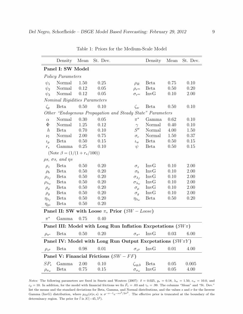
Table 1: Priors for the Medium-Scale Model
Density Mean St. Dev. Density Mean St. Dev.
Panel I: SW Model
Policy Parameters
ψ1 Normal 1.50 0.25 ρR Beta 0.75 0.10ψ2 Normal 0.12 0.05 ρrm Beta 0.50 0.20ψ3 Normal 0.12 0.05 σrm InvG 0.10 2.00
Nominal Rigidities Parameters
ζp Beta 0.50 0.10 ζw Beta 0.50 0.10
Other “Endogenous Propagation and Steady State” Parameters
α Normal 0.30 0.05 π∗ Gamma 0.62 0.10Φ Normal 1.25 0.12 γ Normal 0.40 0.10h Beta 0.70 0.10 S ′′ Normal 4.00 1.50νl Normal 2.00 0.75 σc Normal 1.50 0.37ιp Beta 0.50 0.15 ιw Beta 0.50 0.15r∗ Gamma 0.25 0.10 ψ Beta 0.50 0.15
(Note β = (1/(1 + r∗/100))ρs, σs, and ηs
ρz Beta 0.50 0.20 σz InvG 0.10 2.00ρb Beta 0.50 0.20 σb InvG 0.10 2.00ρλf
Beta 0.50 0.20 σλfInvG 0.10 2.00
ρλw Beta 0.50 0.20 σλw InvG 0.10 2.00ρµ Beta 0.50 0.20 σµ InvG 0.10 2.00ρg Beta 0.50 0.20 σg InvG 0.10 2.00ηλf
Beta 0.50 0.20 ηλw Beta 0.50 0.20ηgz Beta 0.50 0.20
Panel II: SW with Loose π∗ Prior (SW − Loose)
π∗ Gamma 0.75 0.40
Panel III: Model with Long Run Inflation Excpetations (SWπ)
ρπ∗ Beta 0.50 0.20 σπ∗ InvG 0.03 6.00
Panel IV: Model with Long Run Output Excpetations (SWπY )
ρzp Beta 0.98 0.01 σzp InvG 0.01 4.00
Panel V: Financial Frictions (SW − FF )
SP∗ Gamma 2.00 0.10 ζsp,b Beta 0.05 0.005ρσw Beta 0.75 0.15 σσw InvG 0.05 4.00
Notes: The following parameters are fixed in Smets and Wouters (2007): δ = 0.025, g∗ = 0.18, λw = 1.50, εw = 10.0, and
εp = 10. In addition, for the model with financial frictions we fix F∗ = .03 and γ∗ = .99. The columns “Mean” and “St. Dev.”
list the means and the standard deviations for Beta, Gamma, and Normal distributions, and the values s and ν for the Inverse
Gamma (InvG) distribution, where pIG(σ|ν, s) ∝ σ−ν−1e−νs2/2σ2. The effective prior is truncated at the boundary of the
determinacy region. The prior for l is N (−45, 52).
Del Negro, Schorfheide – DSGE Model Based Forecasting: February 29, 2012 10
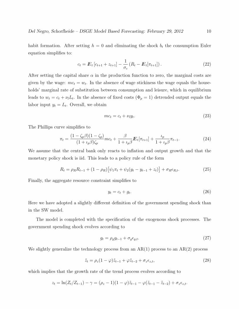
habit formation. After setting h = 0 and eliminating the shock bt the consumption Euler
equation simplifies to:
ct = IEt [ct+1 + zt+1]−1
σc
(Rt − IEt[πt+1]) . (22)
After setting the capital share α in the production function to zero, the marginal costs are
given by the wage: mct = wt. In the absence of wage stickiness the wage equals the house-
holds’ marginal rate of substitution between consumption and leisure, which in equilibrium
leads to wt = ct + νlLt. In the absence of fixed costs (Φp = 1) detrended output equals the
labor input yt = Lt. Overall, we obtain
mct = ct + νlyt. (23)
The Phillips curve simplifies to
πt =(1− ζpβ)(1− ζp)
(1 + ιpβ)ζpmct +
β
1 + ιpβIEt[πt+1] +
ιp1 + ιpβ
πt−1. (24)
We assume that the central bank only reacts to inflation and output growth and that the
monetary policy shock is iid. This leads to a policy rule of the form
Rt = ρRRt−1 + (1− ρR)[ψ1πt + ψ2(yt − yt−1 + zt)
]+ σRεR,t. (25)
Finally, the aggregate resource constraint simplifies to
yt = ct + gt. (26)
Here we have adopted a slightly different definition of the government spending shock than
in the SW model.
The model is completed with the specification of the exogenous shock processes. The
government spending shock evolves according to
gt = ρggt−1 + σgεg,t. (27)
We slightly generalize the technology process from an AR(1) process to an AR(2) process
zt = ρz(1− ϕ)zt−1 + ϕzt−2 + σzεz,t, (28)
which implies that the growth rate of the trend process evolves according to
zt = ln(Zt/Zt−1)− γ = (ρz − 1)(1− ϕ)zt−1 − ϕ(zt−1 − zt−2) + σzεz,t.
Del Negro, Schorfheide – DSGE Model Based Forecasting: February 29, 2012 11
The innovations εz,t, εg,t, and εR,t are assumed to be iid standard normal.
The small-scale model is estimated based on three quarterly macroeconomic time series.
The measurement equations for real output growth, inflation, and interest rates are given
by:
Output growth = γ + 100 (yt − yt−1 + zt)
Inflation = π∗ + 100πt
FFR = R∗ + 100Rt
(29)
where all variables are measured in percent and π∗ and R∗ measure the steady state level
of inflation and short term nominal interest rates, respectively. For the parameters that are
common between the SW model and the small-scale model we use the same marginal prior
distributions as listed in Table 1. The additional parameter ϕz has a prior distribution that
is uniform on the interval (−1, 1) because it is a partial autocorrelation. The joint prior
distribution is given by the products of the marginals, truncated to ensure that the DSGE
model has a determinate equilibrium.
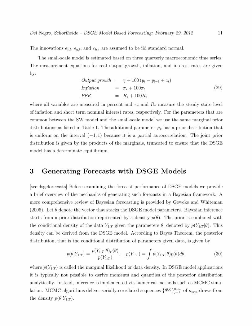
3 Generating Forecasts with DSGE Models
[sec:dsgeforecasts] Before examining the forecast performance of DSGE models we provide
a brief overview of the mechanics of generating such forecasts in a Bayesian framework. A
more comprehensive review of Bayesian forecasting is provided by Geweke and Whiteman
(2006). Let θ denote the vector that stacks the DSGE model parameters. Bayesian inference
starts from a prior distribution represented by a density p(θ). The prior is combined with
the conditional density of the data Y1:T given the parameters θ, denoted by p(Y1:T |θ). This
density can be derived from the DSGE model. According to Bayes Theorem, the posterior
distribution, that is the conditional distribution of parameters given data, is given by
p(θ|Y1:T ) =p(Y1:T |θ)p(θ)p(Y1:T )
, p(Y1:T ) =
∫p(Y1:T |θ)p(θ)dθ, (30)
where p(Y1:T ) is called the marginal likelihood or data density. In DSGE model applications
it is typically not possible to derive moments and quantiles of the posterior distribution
analytically. Instead, inference is implemented via numerical methods such as MCMC simu-
lation. MCMC algorithms deliver serially correlated sequences {θ(j)}nsimj=1 of nsim draws from
the density p(θ|Y1:T ).

Del Negro, Schorfheide – DSGE Model Based Forecasting: February 29, 2012 12
In forecasting applications the posterior distribution p(θ|Y1:T ) is not the primary object
of interest. Instead, the focus is on predictive distributions, which can be decomposed as
follows:
p(YT+1:T+H |Y1:T ) =
∫p(YT+1:T+H |θ, Y1:T )p(θ|Y1:T )dθ. (31)
This decomposition highlights that draws from the predictive density can be obtained by
simulating the DSGE model conditional on posterior parameter draws θ(j) and the observa-
tions Y1;T . In turn, this leads to sequences Y(j)T+1:T+H , j = 1, . . . , nsim that represent draws
from the predictive distribution (31). These draws can then be used to obtain numerical
approximations of moments, quantiles, and the probability density function of YT+1:T+H . In
the remainder of this section, we discuss how to obtain draws from the posterior distribution
of DSGE model parameters (Section 3.1) and how to generate draws from the predictive
distribution of future observations (Section 3.2).
3.1 Posterior Inference for θ
[subsec:posteriortheta] Before the DSGE model can be estimated, it has to be solved using
a numerical method. In most DSGE models, the intertemporal optimization problems of
economic agents can be written recursively, using Bellman equations. In general, the value
and policy functions associated with the optimization problems are nonlinear in terms of
both the state and the control variables, and the solution of the optimization problems
requires numerical techniques. The implied equilibrium law of motion can be written as
st = Φ(st−1, εt; θ), (32)
where st is a vector of suitably defined state variables and εt is a vector that stacks the
innovations for the structural shocks. In this paper, we proceed under the assumption that
the DSGE model’s solution is approximated by log-linearization techniques and ignore the
discrepancy between the nonlinear model solution and the first-order approximation:
st = Φ1(θ)st−1 + Φε(θ)εt. (33)
The system matrices Φ1 and Φε are functions of the DSGE model parameters θ, and st spans
the state variables of the model economy, but also might contain some redundant elements
that facilitate a simple representation of the measurement equation:
yt = Ψ0(θ) + Ψ1(θ)t+ Ψ2(θ)st. (34)

Del Negro, Schorfheide – DSGE Model Based Forecasting: February 29, 2012 13
Equations (33) and (34) provide a state-space representation for the linearized DSGE model.
This representation is the basis for the econometric analysis. If the innovations εt are Gaus-
sian, then the likelihood function p(Y1:T |θ) can be evaluated with a standard Kalman filter.
We now turn to the prior distribution represented by the density p(θ). An example of such
a prior distribution is provided in Table 1. The table characterizes the marginal distribution
of the DSGE model parameters. The joint distribution is then obtained as the product of the
marginals. It is typically truncated to ensure that the DSGE model has a unique solution.
DSGE model parameters can be grouped into three categories: (i) parameters that affect
steady states; (ii) parameters that control the endogenous propagation mechanism of the
model without affecting steady states; and (iii) parameters that determine the law of motion
of the exogenous shock processes.
Priors for steady-state related parameters are often elicited indirectly by ensuring that
model-implied steady states are commensurable with pre-sample averages of the correspond-
ing economic variables. Micro-level information, e.g. about labor supply elasticities or the
frequency of price and wage changes, is often used to formulate priors for parameters that
control the endogenous propagation mechanism of the model. Finally, beliefs about volatili-
ties and autocovariance patterns of endogenous variables can be used to elicit priors for the
remaining parameters. A more detailed discussions and some tools to mechanize the prior
elicitation are provided in Del Negro and Schorfheide (2008).
A detailed discussion of numerical techniques to obtain draws from the posterior distri-
bution p(θ|Y1:T ) can be found, for instance, in An and Schorfheide (2007a) and Del Negro
and Schorfheide (2010). We only provide a brief overview. Because of the nonlinear re-
lationship between the DSGE model parameters θ and the system matrices Ψ0, Ψ1, Ψ2,
Φ1 and Φε of the state-space representation in (33) and (34), the marginal and conditional
distributions of the elements of θ do not fall into the well-known families of probability dis-
tributions. Up to now, the most commonly used procedures for generating draws from the
posterior distribution of θ are the Random-Walk Metropolis (RWM) Algorithm described
in Schorfheide (2000) and Otrok (2001) or the Importance Sampler proposed in DeJong,
Ingram, and Whiteman (2000). The basic RWM Algorithm takes the following form
Algorithm 1. Random-Walk Metropolis (RWM) Algorithm for DSGE Model.
[algo:rwm]

Del Negro, Schorfheide – DSGE Model Based Forecasting: February 29, 2012 14
1. Use a numerical optimization routine to maximize the log posterior, which up to a
constant is given by ln p(Y1:T |θ) + ln p(θ). Denote the posterior mode by θ.
2. Let Σ be the inverse of the (negative) Hessian computed at the posterior mode θ, which
can be computed numerically.
3. Draw θ(0) from N(θ, c20Σ) or directly specify a starting value.
4. For j = 1, . . . , nsim: draw ϑ from the proposal distribution N(θ(j−1), c2Σ). The jump
from θ(j−1) is accepted (θ(j) = ϑ) with probability min {1, r(θ(j−1), ϑ|Y1:T )} and rejected
(θ(j) = θ(j−1)) otherwise. Here,
r(θ(j−1), ϑ|Y1:T ) =p(Y1:T |ϑ)p(ϑ)
p(Y1:T |θ(j−1))p(θ(j−1)). �
If the likelihood can be evaluated with a high degree of precision, then the maximization
in Step 1 can be implemented with a gradient-based numerical optimization routine. The
optimization is often not straightforward because the posterior density is typically not glob-
ally concave. Thus, it is advisable to start the optimization routine from multiple starting
values, which could be drawn from the prior distribution, and then set θ to the value that
attains the highest posterior density across optimization runs. In some applications we found
it useful to skip Steps 1 to 3 by choosing a reasonable starting value, such as the mean of
the prior distribution, and replacing Σ in Step 4 with a matrix whose diagonal elements are
equal to the prior variances of the DSGE model parameters and whose off-diagonal elements
are zero.
While the RWM algorithm in principle delivers consistent approximations of posterior
moments and quantiles even if the posterior contours are highly non-elliptical, the practical
performance can be poor as documented in An and Schorfheide (2007a). Recent research on
posterior simulators tailored toward DSGE models tries to address the shortcomings of the
“default” approaches that are being used in empirical work. An and Schorfheide (2007b)
use transition mixtures to deal with a multi-modal posterior distribution. This approach
works well if the researcher has knowledge about the location of the modes, obtained, for
instance, by finding local maxima of the posterior density with a numerical optimization al-
gorithm. Chib and Ramamurthy (2010) propose to replace the commonly used single block
RWM algorithm with a Metropolis-within-Gibbs algorithm that cycles over multiple, ran-
domly selected blocks of parameters. Kohn, Giordani, and Strid (2010) propose an adaptive

Del Negro, Schorfheide – DSGE Model Based Forecasting: February 29, 2012 15
hybrid Metropolis-Hastings samplers and Herbst (2010) develops a Metropolis-within-Gibbs
algorithm that uses information from the Hessian matrix to construct parameter blocks that
maximize within-block correlations at each iteration and Newton steps to tailor proposal
distributions for the various conditional posteriors.
3.2 Evaluating the Predictive Distribution
[subsec:preddistribution] Bayesian DSGE model forecasts can computed based on draws from
the posterior predictive distribution of YT+1:T+H . We use the parameter draws {θ(j)}nsimj=1
generated with Algorithm 1 in the previous section as a starting point. Since the DSGE
model is represented as a state-space model with latent state vector st, we modify the
decomposition of the predictive density in (31) accordingly:
p(YT+1:T+H |Y1:T ) (35)
=
∫(sT ,θ)
[∫ST+1:T+H
p(YT+1|T+H |ST+1:T+H)p(ST+1:T+H |sT , θ, Y1:T )dST+1:T+H
]×p(sT |θ, Y1:T )p(θ|Y1:T )d(sT , θ)
Draws from the predictive density can be generated with the following algorithm:
Algorithm 2. Draws from the Predictive Distribution. [algo:preddraws] For j = 1 to
nsim, select the j’th draw from the posterior distribution p(θ|Y1:T ) and:
1. Use the Kalman filter to compute mean and variance of the distribution p(sT |θ(j), Y1:T ).
Generate a draw s(j)T from this distribution.
2. A draw from ST+1:T+H |(sT , θ, Y1:T ) is obtained by generating a sequence of innovations
ε(j)T+1:T+H . Then, starting from s
(j)T , iterate the state transition equation (33) with θ
replaced by the draw θ(j) forward to obtain a sequence S(j)T+1:T+H :
s(j)t = Φ1(θ
(j))s(j)t−1 + Φε(θ
(j))ε(j)t , t = T + 1, . . . , T +H.
3. Use the measurement equation (34) to obtain Y(j)T+1:T+H :
y(j)t = Ψ0(θ
(j)) + Ψ1(θ(j))t+ Ψ2(θ
(j))s(j)t , t = T + 1, . . . , T +H. �

Del Negro, Schorfheide – DSGE Model Based Forecasting: February 29, 2012 16
Algorithm 2 generates nsim trajectories Y(j)T+1:T+H from the predictive distribution of
YT+1:T+H given Y1:T . The algorithm could be modified by executing Steps 2 and 3 m times
for each j, which would lead to a total of m · nsim draws from the predictive distribution. A
point forecast yT+h of yT+h can be obtained by specifying a loss function L(yT+h, yT+h) and
determining the prediction that minimizes the posterior expected loss:
yT+h|T = argminδ∈Rn
∫yT+h
L(yT+h, δ)p(yT+h|Y1:T )dyT+h. (36)
For instance, under the quadratic forecast error loss function
L(y, δ) = tr[W (y − δ)′(y − δ)],
where W is a symmetric positive-definite weight matrix and tr[·] is the trace operator, the
optimal predictor is the posterior mean
yT+h|T =
∫yT+h
yT+hp(yT+h|Y1:T )dyT+h ≈1
nsim
nsim∑j=1
y(j)T+h, (37)
which can be approximated by a Monte Carlo average.
Pointwise (meaning for fixed h rather than jointly over multiple horizons) 1−α credible
interval forecasts for a particular element yi,T+h of yT+h can be obtained by either com-
puting the α/2 and 1 − α/2 percentiles of the empirical distribution of {y(j)i,T+h}
nsimj=1 or by
numerically searching for the shortest connected interval that contains a 1−α fraction of the
draws {y(j)i,T+h}
nsimj=1 . By construction, the latter approach leads to sharper interval forecasts.2
Finally, density forecasts can be obtained by applying a density estimator (see Silverman
(1986) for an introduction) to the set of draws {y(j)i,T+h}
nsimj=1 .
As a short-cut, practitioners sometimes replace the numerical integration with respect to
the parameter vector θ in Algorithm 2 by a plug-in step. Draws from the plug-in predictive
distribution p(yT+1:T+H |θ, Y1:T ) are obtained by setting θ(j) = θ in Steps 2 and 3 of the
algorithm. Here θ is a point estimator such as the posterior mode or the posterior mean.
While the plug-in approach tends to reduce the computational burden, it does not deliver
the correct Bayes predictions and, importantly, interval and density forecasts will understate
the uncertainty about future realizations of yt.
2In general, the smallest (in terms of volume) set forecast is given by the highest-density set. If the
predictive density is uni-modal the second above-mentioned approach generates the highest-density set. If
the predictive density is multi-modal, then there might exist a collection of disconnected intervals that
provides a sharper forecast.
Del Negro, Schorfheide – DSGE Model Based Forecasting: February 29, 2012 17
4 Accuracy of Point Forecasts
[sec:pointforecasts] We begin the empirical analysis with the computation of RMSEs for
our DSGE models. The RMSEs are based on a pseudo-out-of-sample forecasting exercise
in which we are using real-time data sets to recursively estimate the DSGE models. The
construction of the real-time data set is discussed in Section 4.1. Empirical results for the
small-scale DSGE model of Section 2.3 are presented in Section 4.2. We compare DSGE
model-based RMSEs to RMSEs computed for forecasts of the Blue Chip survey. A similar
analysis is conducted for the SW model in Section 4.3. Finally, Section 4.4 summarizes results
on the forecast performance of medium-scale DSGE models published in the literature.
4.1 A Real Time Data Set for Forecast Evaluation
[subsec:realtimedata] Since the small-scale DSGE model is estimated based on a subset of
variables that are used for the estimation of the SW model, we focus on the description of
the data set for the latter. Real GDP (GDPC), the GDP price deflator (GDPDEF), nominal
personal consumption expenditures (PCEC), and nominal fixed private investment (FPI) are
constructed at a quarterly frequency by the Bureau of Economic Analysis (BEA), and are
included in the National Income and Product Accounts (NIPA).
Average weekly hours of production and nonsupervisory employees for total private in-
dustries (PRS85006023), civilian employment (CE16OV), and civilian noninstitutional pop-
ulation (LNSINDEX) are produced by the Bureau of Labor Statistics (BLS) at the monthly
frequency. The first of these series is obtained from the Establishment Survey, and the re-
maining from the Household Survey. Both surveys are released in the BLS Employment Sit-
uation Summary (ESS). Since our models are estimated on quarterly data, we take averages
of the monthly data. Compensation per hour for the nonfarm business sector (PRS85006103)
is obtained from the Labor Productivity and Costs (LPC) release, and produced by the BLS
at the quarterly frequency.
Last, the federal funds rate is obtained from the Federal Reserve Board’s H.15 release at
the business day frequency, and is not revised. We take quarterly averages of the annualized

Del Negro, Schorfheide – DSGE Model Based Forecasting: February 29, 2012 18
daily data. All data are transformed following Smets and Wouters (2007). Specifically:
Output growth = LN((GDPC)/LNSINDEX) ∗ 100
Consumption growth = LN((PCEC/GDPDEF )/LNSINDEX) ∗ 100
Investment growth = LN((FPI/GDPDEF )/LNSINDEX) ∗ 100
Real Wage growth = LN(PRS85006103/GDPDEF ) ∗ 100
Hours = LN((PRS85006023 ∗ CE16OV/100)/LNSINDEX) ∗ 100
Inflation = LN(GDPDEF/GDPDEF (−1)) ∗ 100
FFR = FEDERAL FUNDS RATE/4
In the estimation of the DSGE model with financial frictions we measure Spread as the
annualized Moody’s Seasoned Baa Corporate Bond Yield spread over the 10-Year Treasury
Note Yield at Constant Maturity. Both series are available from the Federal Reserve Board’s
H.15 release, and averaged over each quarter. Spread data is also not revised.
Many macroeconomic time series get revised multiple times by the statistical agencies
that publish the series. In many cases the revisions reflect additional information that has
been collected by the agencies, in other instances revisions are caused by changes in defi-
nitions. For instance, the BEA publishes three releases of quarterly GDP in the first three
month following the quarter. Thus, in order to be able to compare DSGE model forecasts
to real-time forecasts made by private-sector professional forecasters or the Federal Reserve
Board, it is important to construct vintages of real time historical data. We follow the work
by Edge and Gurkaynak (2010) and construct data vintages that are aligned with the publi-
cation dates of the Blue Chip survey and the Federal Reserve Board’s Greenbook/Tealbook.
Blue Chip’s survey of professional forecasters is published on the 10th of each month,
based on responses that have been submitted at the end of the previous month. For instance,
forecasts published on April 10 are based on information that was available at the end of
March. Whenever we evaluate the accuracy of Blue Chip forecasts in this paper, we focus
on the so-called Consensus Blue Chip forecast, which is defined as the average of all the
forecasts gathered in the Blue Chip Economic Indicators (BCEI) survey. While there are
three Blue Chip forecasts published every quarter, we restrict our attention to the month
in which the last forecast is made in each quarter. Given the approximate two week delay
between the survey and the publication of the results on the 10th of each month, this means
that we are constructing data sets that are aligned with the information available for the
January, April, July, and October Blue Chip publications. For concreteness, consider the

Del Negro, Schorfheide – DSGE Model Based Forecasting: February 29, 2012 19
April 1992 Blue Chip release date. In late March the NIPA series for 1992:Q1 are not yet
available, which means that the DSGE model can only be estimated based on a sample that
ends in 1991:Q4. Our selection of Blue Chip dates maximizes the informational advantage
for the Blue Chip forecasters, who can in principle utilize high-frequency information about
economic activity in 1992:Q1 that is available by late March. The first forecast origin con-
sidered in the subsequent forecast evaluation is January 1992 and the last one is April 2011.
We refer to the collection of data vintages aligned with the Blue Chip publication dates as
Blue Chip sample.
The Greenbook/Tealbook contains macroeconomic forecasts from the staff of the Board
of Governors in preparation for a FOMC meeting. There are typically eight FOMC meetings
per year. For the comparison of Greenbook versus DSGE model forecasts we also only
consider a subset of four Greenbook publication dates, one associated with each quarter:
typically from the months of March, June, September, and December.3 We refer to the
collection of vintages aligned with the Greenbook dates as Greenbook sample. The first
forecast origin in the Greenbook sample is March 1992 and the last one is September 2004,
since the Greenbook forecasts are only available with a 5 year lag. Table 2 summarizes
the Blue Chip and Greenbook forecast origins in 1992 for which we are constructing DSGE
model forecasts. Since we always use real time information, the vintage used to estimate the
DSGE model for the comparison to the March 1992 Greenbook may be different from the
vintage that is used for the comparison with the April 1992 Blue Chip forecast, even though
in both cases the end of the estimation sample for the DSGE model is T=1991:Q4.
The Blue Chip Economic Indicators survey only contain quarterly forecasts for one calen-
dar year after the current one. This implies that on January 10 the survey will have forecasts
for eight quarters, and only for six quarters on October 10. When comparing forecast accu-
racy between Blue Chip and DSGE models, we use seven- and eight-quarter ahead forecasts
only when available from the Blue Chip survey (which means we only use the January and
April forecast dates when computing eight-quarter ahead RMSEs). For consistency, when
comparing forecast accuracy across DSGE models we use the same approach (we refer to this
set of dates/forecast horizons as the “Blue Chip dates”). Similarly, the horizon of Greenbook
3As forecast origins we choose the last Greenbook forecast date before an advanced NIPA estimate for
the most recent quarter is released. For instance, the advanced estimate for Q1 GDP is typically released in
the second half of April, prior to the April FOMC meeting.

Del Negro, Schorfheide – DSGE Model Based Forecasting: February 29, 2012 20
Table 2: Blue Chip and Greenbook Forecast Dates for 1992
Forecast Origin End of Est. Forecast
Blue Chip Greenbook Sample T h = 1 h = 2 h = 3 h = 4
Apr 92 Mar 92 91:Q4 92:Q1 92:Q2 92:Q3 92:Q4
Jul 92 Jun 92 92:Q1 92:Q2 92:Q3 92:Q4 93:Q1
Oct 92 Sep 92 92:Q2 92:Q3 92:Q4 93:Q1 93:Q2
Jan 93 Dec 92 92:Q3 92:Q4 93:Q1 93:Q2 93:Q3
forecasts also varies over time. In comparing DSGE model and Greenbook forecast accuracy
we only use seven- and eight-quarter ahead whenever available from both.
For each forecast origin our estimation sample begins in 1964:Q1 and ends with the
most recent quarter for which a NIPA release is available. Historical data were taken from
the FRB St. Louis’ ALFRED database. For vintages prior to 1997, compensation and
population series were unavailable in ALFRED. In these cases, the series were taken from
Edge and Gurkaynak (2010).4 In constructing the real time data set, the release of one
series for a given quarter may outpace that of another. For example, in several instances,
Greenbook forecast dates occur after a quarter’s ESS release but before the NIPA release.
In other words, for a number of data vintages there is, relative to NIPA, an extra quarter
of employment data. Conversely, in a few cases NIPA releases outpace LPC, resulting in
an extra quarter of NIPA data. We follow the convention in Edge and Gurkaynak (2010)
and use NIPA availability to determine whether a given quarter’s data should be included in
a vintage’s estimation sample. When employment data outpace NIPA releases, this means
ignoring the extra observations for hours, population, and employment from the Employment
Situation Summary. In cases where NIPA releases outpace LPC releases, we include the next
available LPC data in that vintage’s estimation sample to “catch up” to the NIPA data.
There is an ongoing debate in the forecasting literature as to whether the “actuals”
used in computing forecast errors should be the values of the variables according to the
last available vintage, or the so-called “first finals”, which for output corresponds with the
4We are very grateful to Rochelle Edge and Refet Gurkaynak for giving us this data, and explaining us
how they constructed their dataset.

Del Negro, Schorfheide – DSGE Model Based Forecasting: February 29, 2012 21
“Final” NIPA estimate (available roughly three months after the quarter is over). We show
results according to the first approach.
Finally, the various DSGE models only produce forecasts for per-capita output, while
Blue Chip and Greenbook forecasts are in terms of total GDP. When comparing RMSEs
between the DSGE models and Blue Chip/Greenbook we therefore transform per-capita
into aggregate output forecasts using (the final estimate of) realized population growth.5
4.2 Forecasts from the Small-Scale Model
[subsec:rmsesmallmodel] We begin by comparing the point forecast performance of the small-
scale DSGE model described in Section 2.3 to that of the Blue Chip and Greenbook forecasts.
RMSEs for output growth, inflation, and interest rates (Federal Funds) are displayed in
Figure 1. Throughout this paper, GDP growth rates, inflation rates, and interest rates are
reported in Quarter-on-Quarter (QoQ) percentages. The RMSEs in the first row of the figure
are for forecasts that are based on the information available prior to the January, April, July,
and October Blue Chip publication dates over the period 1992 to 2011. The RMSEs in the
bottom row correspond to forecasts generated at the March, June, September, and December
Greenbook dates over the period from 1992 to 2004.
The small-scale model attains a RMSE for output growth of approximately 0.65%. The
RMSE is fairly flat with respect to the forecast horizon, which is consistent with the low
serial correlation of U.S. GDP growth. At the nowcast horizon (h = 1), the Blue Chip
forecasts are much more precise, their RMSE is 0.42, because they incorporate information
from the current quarter. As the forecast horizon increases to h = 4 the RMSEs of the DSGE
model and the Blue Chip forecasts are approximately the same. The accuracy of inflation
and, in particular, interest rate forecasts of the small scale DSGE model is decreasing in the
forecast horizon h due to the persistence of these series. The inflation RMSE is about 0.25%
at the nowcast horizon and 0.35% for a two-year horizon. For the Federal Funds rate the
RMSE increases from about 0.15 to 0.5. The inflation and interest rate Blue Chip forecasts
tend to be substantially more precise than the DSGE model forecasts both at the nowcast
as well as the one-year horizon.
5Edge and Gurkaynak (2010) follow a similar approach, except that their population “actuals” are the
“first finals”, consistently with the fact that they use “first finals” to measure forecast errors.

Del Negro, Schorfheide – DSGE Model Based Forecasting: February 29, 2012 22
In comparison to the Greenbook forecasts the output growth forecasts of the small-scale
DSGE model are more precise for horizons h ≥ 3. Moreover, the inflation forecast of the
DSGE model at the nowcast horizon is about as precise as the Greenbook inflation nowcast,
but for horizons h ≥ 1 the Greenbook forecasts dominate. We do not report RMSEs for
Greenbook interest rate projections because the FOMC sets the nominal interest rate in part
based on the information provided in the Greenbook.
4.3 Forecasts from the Smets-Wouters Model
[subsec:rmsemediummodel] We proceed by computing forecast error statistics for the SW
model reviewed in Section 2.1. The results are reported in Figure 2. The top panels provide
a comparison to Blue Chip forecasts from 1992 to 2011 and the bottom panels a comparison
to Greenbook forecasts from 1992 to 2004. The accuracy of the output growth and inflation
forecasts from the SW model forecasts for the Blue Chip dates is commensurable with the
accuracy of the forecasts generated by the small-scale DSGE model. The inflation forecast
of the SW model, however, are more precise than the inflation forecasts of the small-scale
model, which can be attributed to a more sophisticated Phillips curve relationship and the
presence of wage stickiness. The SW interest rate forecasts are slightly more accurate in the
short run but slightly less precise in the long run. In the short-run the Blue Chip forecasts of
output growth and inflation are more precise than the forecasts from the SW model, but for
horizons h = 5 to h = 8, the DSGE model dominates. In general the DSGE model forecast
errors are smaller for the Greenbook sample than for the Blue Chip sample. While the Blue
Chip sample spans the period from 1992 to 2011, the forecasts for the Greenbook sample
end in 2004 and thereby exclude the most recent recession. Except at the nowcast horizon,
the SW model produces slightly more precise point forecasts than the Greenbook, though
the differences in forecast accuracy tend to be small.
Up to this point we considered multi-step-ahead forecasts of growth rates of output and
prices, as well as multi-step-ahead forecast of interest rates. Alternatively, the model can
be used to forecast average growth rates and average interest rates over the next h-periods.
In many instance, forecasts of averages might be more appealing than forecasts of a growth
rate between period T +h− 1 and T +h. RMSEs associated with forecasts of averages tend
to have a different profile as a function of h. To fix ideas, suppose that yt, say inflation,

Del Negro, Schorfheide – DSGE Model Based Forecasting: February 29, 2012 23
Figure 1: RMSEs for Small-Scale Model
DSGE vs Blue Chip (1992-2011)
Output Growth Inflation Interest Rates
1 2 3 4 5 6 7 80.4
0.45
0.5
0.55
0.6
0.65
0.7
0.75
1 2 3 4 5 6 7 80.15
0.2
0.25
0.3
0.35
1 2 3 4 5 6 7 80
0.15
0.3
0.45
0.6
0.75
SMODBC
DSGE vs Greenbook (1992-2004)
Output Growth Inflation Interest Rates
1 2 3 4 5 6 7 80.4
0.45
0.5
0.55
0.6
0.65
0.7
0.75
1 2 3 4 5 6 7 80.15
0.2
0.25
0.3
0.35
1 2 3 4 5 6 7 80
0.15
0.3
0.45
0.6
0.75
SMODGB
Notes: The top and bottom panels compare the RMSEs for the Small-Scale DSGE model (circles) with the Blue Chip (blue
diamonds, top panel) and Greenbook (green diamonds, bottom panel) for one through eight quarters ahead for output growth,
inflation, and interest rates. All variables are expressed in terms of QoQ rates in percentage. Section 4.1 provides the details
of the forecast comparison exercise.

Del Negro, Schorfheide – DSGE Model Based Forecasting: February 29, 2012 24
Figure 2: RMSEs for SW Model
DSGE vs Blue Chip (1992-2011)
Output Growth Inflation Interest Rates
1 2 3 4 5 6 7 80.4
0.45
0.5
0.55
0.6
0.65
0.7
0.75
1 2 3 4 5 6 7 80.15
0.2
0.25
0.3
0.35
1 2 3 4 5 6 7 80
0.15
0.3
0.45
0.6
0.75
SWBC
DSGE vs Greenbook (1992-2004)
Output Growth Inflation Interest Rates
1 2 3 4 5 6 7 80.4
0.45
0.5
0.55
0.6
0.65
0.7
0.75
1 2 3 4 5 6 7 80.15
0.2
0.25
0.3
0.35
1 2 3 4 5 6 7 80
0.15
0.3
0.45
0.6
0.75
SWGB
Notes: The top and bottom panels compare the RMSEs for the SW DSGE model (circles) with the Blue Chip (blue diamonds,
top panel) and Greenbook (green diamonds, bottom panel) for one through eight quarters ahead for output growth, inflation,
and interest rates. All variables are expressed in terms of QoQ rates in percentage. Section 4.1 provides the details of the
forecast comparison exercise.
evolves according to an AR(1) process
yt = θyt−1 + ut, ut ∼ iidN(0, 1), 0 < θ < 1. (38)

Del Negro, Schorfheide – DSGE Model Based Forecasting: February 29, 2012 25
To simplify the exposition, we will abstract from parameter uncertainty and assume that θ
is known. The time T h-step forecast of yT+h is given by yT+h|T = θhyT . The h-step ahead
forecast error is given by
eT+h|T =h−1∑j=0
θjuT+h−j. (39)
In turn, the population RMSE is given by√E[e2T+h|T ] =
√1− θ2h
1− θ2−→ 1√
1− θ2as h→∞. (40)
If θ is close to zero, the RMSE as a function of h is fairly flat, whereas it is strongly increasing
for values of θ close to one. The RMSEs associated with the DSGE model forecasts aligned
with the Blue Chip publication dates in the top panels of Figure 2 are broadly consistent
with this pattern. The serial correlation of output growth and inflation is fairly small, which
leads to a fairly flat, albeit slightly increasing RMSE function. Interest rates, on the other
hand, follow a highly persistent process (θ ≈ 1), which generates RMSEs that are essentially
linearly increasing in the forecast horizon.
The error associated with a forecast of an h-period average is given by
eT+h|T =1
h
h∑s=1
(s−1∑j=0
θjuT+s−j
)=
1
h
h−1∑j=0
1− θj+1
1− θut+h−j. (41)
The second equality is obtained by re-arranging terms and using the formula∑j−1
s=0 θs =
(1− θj)/(1− θ). The resulting population RMSE is given by
√E[e2T+h|T ] =
1√h(1− θ)2
√1− 2θ
1− θh
h(1− θ)+ θ2
1− θ2h
h(1− θ2). (42)
Thus, the RMSE of the forecast of the h-period average decays at rate 1/√h. Based on
results from the Blue Chip sample, we plot RMSEs for the forecasts of average output
growth, average inflation, and average interest rates in Figure 3. In assessing the empirical
results, it is important to keep in mind that the population RMSE calculated above abstracts
from parameter uncertainty and potential misspecification of the forecasting model. The
GDP growth and inflation RMSEs for the DSGE model are indeed decreasing in the forecast
horizon. The interest rate RMSEs remain increasing in h, but compared to Figure 2 the
slope is not as steep. Since the Blue Chip forecasts are more precise at short horizons, the
averaging favors the Blue Chip forecasts in the RMSE comparison.

Del Negro, Schorfheide – DSGE Model Based Forecasting: February 29, 2012 26
Figure 3: RMSEs for SW Model vs Blue Chip: Forecasting Averages
Forecasts of h-Period Averages
Output Growth Inflation Interest Rates
1 2 3 4 5 6 7 80.35
0.4
0.45
0.5
0.55
0.6
0.65
0.7
1 2 3 4 5 6 7 80.18
0.19
0.2
0.21
0.22
0.23
0.24
0.25
0.26
0.27
1 2 3 4 5 6 7 80
0.05
0.1
0.15
0.2
0.25
0.3
0.35
0.4
SWBC
Notes: The figure compares the RMSEs for the SW DSGE model (circles) with the Blue Chip forecasts (blue diamonds) for
one through eight quarters-ahead averages for output growth, inflation, and interest rates. All variables are expressed in terms
of QoQ rates in percentage. Section 4.1 provides the details of the forecast comparison exercise.
4.4 Literature Review of Forecasting Performance
[subsec:rmseliterature] By now there exists a substantial body of research evaluating the
accuracy of point forecasts from DSGE models. Some of the papers are listed in Table 3.
Many of the studies consider variants of the Smets and Wouters (2003, 2007) models. Since
the studies differ with respect to the forecast periods, that is, the collection of forecast origins,
as well as the choice of data vintages, direct comparisons of results are difficult. Smets and
Wouters (2007) report output growth, inflation, and interest rate RMSEs of 0.57%, 0.24%,
and 0.11% QoQ. The forecast period considered by Smets and Wouters (2007) ranges from
1990:Q1 to 2004:Q2 and is comparable to our Greenbook sample. The corresponding RMSEs
obtained in our analysis in Section 4.3 using real-time data are 0.55%, 0.19%, and 0.11%.
In order to make the RMSE results comparable across studies we generate forecasts from
a simple AR(2), using the variable definitions, forecast origins, and estimation samples that
underly the studies listed in Table 3. In particular, we use real-time data whenever the
original study was based on real-time data and we use the corresponding vintage for studies
that were based on the analysis of a single vintage. The AR(2) model is estimated using

Del Negro, Schorfheide – DSGE Model Based Forecasting: February 29, 2012 27
Table 3: A Sample of Studies Reporting RMSEs for Medium-Scale DSGE Models
Study Forecast Origins Real Time
Rubaszek and Skrzypczynski (2008) 1994:Q1 - 2005:Q3 Yes
Kolasa, Rubaszek, and Skrzypczynski (2010) 1994:Q1 - 2007:Q4 Yes
Graeve, Emiris, and Wouters (2009) 1990:Q1 - 2007:Q1 (h=1) No
Wolters (2010), Del Negro-Schorfheide Model 1984:Q1 - 2000:Q4 Yes
Wolters (2010), Fuhrer-Moore Model 1984:Q1 - 2000:Q4 Yes
Wolters (2010), SW Model 1984:Q1 - 2000:Q4 Yes
Wolters (2010), EDO Model 1984:Q1 - 2000:Q4 Yes
Edge and Gurkaynak (2010) 1992:Jan - 2004:Q4 Yes
Edge, Kiley, and Laforte (2009) 1996:Sep - 2002:Q4 Yes
Smets and Wouters (2007) 1990:Q1 - 2004:Q4 (h=1) No
Del Negro, Schorfheide, Smets, and Wouters (2007) 1985:Q4 - 2000:Q2 (h=1) No
Schorfheide, Sill, and Kryshko (2010) 2001:Q1 - 2007:Q4 (h=1) No

Del Negro, Schorfheide – DSGE Model Based Forecasting: February 29, 2012 28
Bayesian techniques with the improper prior p(σ2) ∝ (σ2)−1, where σ2 is the innovation
variance.
Figure 4 depicts RMSE ratios for DSGE model forecasts versus AR(2) forecasts. Each
cross corresponds to one of the studies listed in Table 3. A value less than one indicates
that the RMSE of the DSGE model forecast is lower than the RMSE of the benchmark
AR(2) forecast. The solid lines indicate RMSE ratios of one. The top panels summarize the
accuracy of output growth and inflation forecasts, whereas the bottom panel summarize the
accuracy of interest rate and inflation forecasts. In general, the DSGE models perform better
at the h = 4 horizon than at the one-quarter-ahead horizon as there are fewer observations
in the upper-right quadrant.
While the one-step-ahead output growth forecasts from the DSGE models are by and
large at par with the AR(2) forecasts, the bottom left panel indicates that the DSGE model
inflation and interest rate forecasts in general tend to be worse than the AR(2) forecasts. At
the one-year horizon, more than half of the DSGE model output growth forecasts are more
accurate than the corresponding AR(2) forecasts. One outlier (the RMSE ratio is close to
2.0) is the output growth RMSE reported in Del Negro, Schorfheide, Smets, and Wouters
(2007), which is computed from an infinite-order VAR approximation of the state-space
representation of the DSGE model. Growth rate differentials between output, investment,
consumption, and real wages might contribute to the poor forecast performance of the DSGE
model. Finally, about half of the estimated DSGE models considered here are able to produce
inflation and interest rate forecasts that attain a lower RMSE than the AR(2) forecasts.
Our interpretation of Figure 4 is that DSGE model forecasts can be competitive in
terms of accuracy with simple benchmark models, in particular for medium-run forecasts.
This statement, however, has two qualifications. First, the DSGE model needs to carefully
specified to optimize forecast performance. Second, if the AR(2) model is replaced by a
statistical model that is specifically designed to forecast a particular macroeconomic time
series well, DSGE model forecasts can be dominated in terms of RMSEs by other time series
models.
Many of the papers in the DSGE model forecasting literature offer direct comparisons of
DSGE model forecasts to other forecasts. Edge and Gurkaynak (2010) compare univariate
forecasts from the SW model estimated with real-time data against forecasts obtained from

Del Negro, Schorfheide – DSGE Model Based Forecasting: February 29, 2012 29
Figure 4: RMSEs Reported in the Literature
Notes: Figure depicts RMSE ratios: DSGE (reported in various papers) / AR(2) (authors
calculation).

Del Negro, Schorfheide – DSGE Model Based Forecasting: February 29, 2012 30
the staff of the Federal Reserve, the Blue Chip survey, and a Bayesian vector autoregres-
sion (VAR). Based on RMSEs, they conclude that the DSGE model delivers forecasts that
are competitive in terms of accuracy with those obtained from the alternative prediction
methods. Comparisons between DSGE model and professional forecasts are also reported
in Wieland and Wolters (2011) and Wieland and Wolters (2012). The evidence from Euro
Area data is similar. Adolfson, Linde, and Villani (2007) assess the forecasting performance
of an Open Economy DSGE model during the period of 1994 to 2004 based on RMSEs, log
determinant of the forecast-error covariance matrix6, predictive scores, and the coverage fre-
quency of interval forecasts. Overall, the authors conclude that the DSGE model compares
well with more flexible time series models such as VARs.
Christoffel, Coenen, and Warne (2010) examine the forecasting performance of the New
Area Wide Model (NAWM), the DSGE model used by the European Central Bank. The
authors evaluate the model’s univariate forecast performance through RMSEs and its multi-
variate performance using the ln-det statistic. They find that the DSGE model is competitive
with other forecasting models such as VARs of various sizes. The authors also find that the
assessment of multivariate forecasts based on the ln-det statistic can sometimes be severely
affected by the inability to forecast just one series, nominal wage growth.
The Bayesian VARs that serve as a benchmark in the aforementioned papers use a
Minnesota prior but are typically not optimized with respect to their empirical performance.
For instance, some of the dummy observations described in Sims and Zha (1998) and more
recently discussed in Del Negro and Schorfheide (2010) that generate a priori correlations
among VAR coefficients and have been found useful for prediction have been excluded from
the construction of the prior distribution. Del Negro and Schorfheide (2004) and DSSW
compare the forecasting performance of a three-equation New Keynesian DSGE model and
a variant of the SW model to Bayesian VARs that use a prior distribution centered at
the DSGE model restrictions. Both papers find that the resulting DSGE-VAR forecasts
significantly better than the underlying DSGE model.
In addition to comparing point forecasts across different models, Edge and Gurkaynak
6The so-called “ln-det” statistic had been proposed by Doan, Litterman, and Sims (1984). The eigen-
vectors of the forecast error covariance matrix generate linear combinations of the model variables with
uncorrelated forecast errors. The determinant equals the product of the eigenvalues and thereby measures
the product of the forecast error variances associated with these linear combinations. The more linear
combinations exist that can be predicted with small forecast error variance, the smaller the ln-det statistic.

Del Negro, Schorfheide – DSGE Model Based Forecasting: February 29, 2012 31
(2010) also examine the overall quality of DSGE model forecasts. To do so, they estimate
regressions of the form
yi,t = α(h) + β(h)yi,t|t−h + e(h)t . (43)
If the predictor yi,t|t−h is the conditional mean of yi,t then the estimate of α(h) should be close
to zero and the estimate of β(h) close to one. In the simple AR(1) example in Equation (38)
of Section 4.3 the residual e(h)t would be equal to the h-step-ahead forecast error et|t−h
in (39) and the population R2 of the regression (43) would be θ2h. For inflation forecasts of
varying horizons h Edge and Gurkaynak (2010) find that α(h) is significantly positive, β(h)
is significantly less than one, and R2 is near zero. The output growth forecasts are better
behaved in that the authors are unable to reject the hypotheses that α(h) = 0 and β(h) = 1.
Moreover, R2 is between 0.07 and 0.2. While the fairly low R2 is qualitatively consistent
with the low persistent in inflation and output growth during the forecasting period, the
estimates of α(h) and β(h) indicate that the DSGE model forecasts are deficient.
Herbst and Schorfheide (2011) examine whether the realized pseudo-out-of-sample RMSE
of DSGE model forecasts is commensurable with the RMSE that would be expected given the
posterior distribution of DSGE model parameters. By simulating the estimated DSGE model
and then generating recursive forecasts on the simulated trajectories, one can obtain a DSGE
model-implied predictive distribution for RMSEs. The authors find that for a small-scale
DSGE model, similar to the model of Section 2.3, the actual RMSEs of output and inflation
forecasts are within the bands of the predictive distribution. The actual interest rate RMSEs,
on the other hand, exceed the predictive bands, indicating a deficiency in the law of motion
of the interest rate. For the Smets and Wouters (2007) model, the inflation and interest rate
RMSEs fall within the bands of the predictive distribution, but the realized output growth
RMSE is smaller than the RMSE predicted by the model. A possible explanation is that
some of the estimated shock processes are overly persistent because they need to absorb
violations of the balanced growth path restrictions of the DSGE model. This would lead to
excess volatility in the simulated output paths.
To summarize, the empirical evidence supports our claim that DSGE model forecasts are
comparable to standard autoregressive or vector autoregressive models but can be dominated
by more sophisticated univariate or multivariate time series. Nonetheless DSGE models
present advantages relative to reduced form models as tools for predictions because they
provide an intelligible econonomic story for their projections, as we discuss in Section 7.
Del Negro, Schorfheide – DSGE Model Based Forecasting: February 29, 2012 32
Moreover, these models also provide a framework for policy analysis. In the forecasting
context this is important as they can be used to make projections based on alternative paths
for the policy instrument (see Section 6).
5 DSGE Model Forecasts using External Information
[sec:externalinfo] In the previous section we generated baseline forecasts from two DSGE
models. For the small-scale model these forecasts were based on output growth, inflation,
and interest rate data. For the SW model we also used data on consumption, investment,
hours worked, and real wages. However, these series reflect only a subset of the information
that is available to a forecaster in real time. While quarterly NIPA data are released with
a lag of more than four weeks, other series, e.g. interest rates, are observed at a much
higher frequency and without publication lag. Thus, in this section we present methods of
improving DSGE model forecasts by incorporating what we call external information. This
external information can take various forms. We consider long-run inflation expectations
(Section 5.1), long-run output growth expectations (Section 5.2), nowcasts of output and
inflation from professional forecasters (Section 5.3), as well as expectations of the short-term
interest rate over various horizons (Section 5.4).
Two distinctly different approaches of incorporating the external information are con-
sidered. First, in Sections 5.1, 5.2, and 5.4 we treat some of the (rational) expectations held
by agents within the DSGE model as observable and equate them with multi-step forecasts
published by the Blue Chip Survey. Discrepancies between DSGE-model implied expecta-
tions and professional forecasts are bridged by introducing additional structural shocks into
the DSGE models presented in Section 2: shocks to the target inflation rate, the growth rate
of technology, and anticipated monetary policy shocks. Second, in Section 5.3 we consider
methods that amount to interpreting nowcasts from professional forecasters as a noisy mea-
sure of (or as news about) current quarter macroeconomic variables. In turn, the external
nowcasts provide information about the exogenous shocks that hit the economy in the cur-
rent quarter and thereby alter the DSGE model forecasts. These methods do not require
the DSGE model to be modified and augmented by additional structural shocks.

Del Negro, Schorfheide – DSGE Model Based Forecasting: February 29, 2012 33
5.1 Incorporating Long-Run Inflation Expectations
[subsec:inflationexpectations] The level of inflation and interest rates has shifted substantially
in the post-war period. In our DSGE models the estimated target inflation rate roughly
corresponds to the sample average of the inflation rate. If the sample includes observations
from the 70s and 80s, then this sample average tends to be higher than what can be thought
of as a long-run inflation target of the past decade, which is around 2%. In turn, this leads
to a poor forecast performance.
In Figure 5 we are plotting the RMSE of the output growth, inflation, and interest rate
forecasts from the SW model under the prior distribution used in Smets and Wouters (2007)
as well as an alternative prior. The original prior for the quarterly steady state inflation rate
used by Smets and Wouters (2007) is tightly centered around 0.62% (which is about 2.5%
annualized) with a standard deviation of 0.1%. Our alternative prior is centered at 0.75%
and is less dogmatic with a standard deviation of 0.4% (see Panel II of Table 1). We refer
to the model with “loose” prior as SW-Loose. Under the Smets and Wouters (2007) prior
the estimated target inflation rate is around 2.7% to 3.0%, whereas the “loose” prior yields
posterior estimates in the range of 4% to 5% As a consequence, the medium-run forecast
accuracy is worse for the SW-Loose model than for the SW model, in particular for inflation
but also for interest rates and output growth.
The forecast inaccuracy caused by the gradual decline of inflation and interest rates post
1980 had been recognized by Wright (2011), who proposed to center the prior distribution
for the vector of long-run means in a Bayesian VAR at the five-to-ten year expectations of
professional forecasters. This approach turned out to be particularly helpful for inflation
forecasts, because of the ability of survey forecasts to capture shifting end points. Faust and
Wright (2011) use a similar approach to improve inflation forecasts from a DSGE model.
Instead of simply centering a tight prior for π∗ with hindsight, they center the prior at the
most recent long-run inflation forecast.
Our approach is similar in spirit to Faust and Wright (2011), but differs in regard to
the implementation. In order to capture the rise and fall of inflation and interest rates in
the estimation sample we replace the constant target inflation rate by a time-varying target
inflation. While time-varying target rates have been frequently used for the specification of
monetary policy rules in DSGE model (e.g., Erceg and Levin (2003), Smets and Wouters

Del Negro, Schorfheide – DSGE Model Based Forecasting: February 29, 2012 34
Figure 5: Using Inflation Expectations
SW vs SW with “loose” prior (SW-Loose)vs SW with “loose” prior and long run inflation expectations (SWπ)
Output Growth Inflation Interest Rates
1 2 3 4 5 6 7 80.4
0.45
0.5
0.55
0.6
0.65
0.7
0.75
1 2 3 4 5 6 7 80.15
0.2
0.25
0.3
0.35
1 2 3 4 5 6 7 80
0.15
0.3
0.45
0.6
0.75
SWSW−LooseSWπ
Notes: The figure compares the one through eight quarters-ahead RMSEs for the SW DSGE model (SW, circles) with the SW
model with a “loose” prior on the parameter π∗ (SW-Loose, crosses) and the SW model with observed long run inflation expec-
tations (SWπ, squares) for output growth, inflation, and interest rates. The comparison is done for the same vintages/forecast
dates as the Blue Chip/DSGE comparison discussed in Section 4.3. All variables are expressed in terms of QoQ rates in
percentage. Section 4.1 provides the details of the forecast comparison exercise.
(2003) and Justiniano, Primiceri, and Tambalotti (2009), among others), we follow the ap-
proach of Aruoba and Schorfheide (2010) and Del Negro and Eusepi (2011) and include data
on long-run inflation expectations as an observable into the estimation of the DSGE model.
At each point in time, the long-run inflation expectations essentially determine the level of
the target inflation rate.
More specifically, for the SW model the interest-rate feedback rule of the central bank (16)
is modified as follows:7
Rt = ρRRt−1 + (1− ρR)(ψ1(πt − π∗t ) + ψ2(yt − yf
t ))
(44)
+ψ3
((yt − yf
t )− (yt−1 − yft−1))
+ rmt .
7We follow the specification in Del Negro and Eusepi (2011), while Aruoba and Schorfheide (2010) assume
that the inflation target also affects the intercept in the feedback rule.

Del Negro, Schorfheide – DSGE Model Based Forecasting: February 29, 2012 35
The time-varying inflation target evolves according to:
π∗t = ρπ∗π∗t−1 + σπ∗επ∗,t, (45)
where 0 < ρπ∗ < 1 and επ∗,t is an iid shock. We follow Erceg and Levin (2003) and model
π∗t as following a stationary process, although our prior for ρπ∗ will force this process to
be highly persistent (see Panel III of Table 1). The set of measurement equations (17) is
augmented by
πO,40t = π∗ + 100IEt
[1
40
40∑k=1
πt+k
](46)
= π∗ +100
40Ψ2(θ)(π,.)(I − Φ1(θ))
−1(Φ1(θ)− Φ1(θ)
41)st,
where πO,40t represents observed long run inflation expectations obtained from surveys (in
percent per quarter), and the right-hand-side of (46) corresponds to expectations obtained
from the DSGE model (in deviation from the mean π∗). The second line shows how to
compute these expectations using the transition equation (33), where Ψ2(θ)(π,.) is the row of
the matrix Ψ2(θ) entering the measurement equation (34) corresponding to inflation.
The long-run inflation forecasts are obtained from the Blue Chip Economic Indicators
survey and the Survey of Professional Forecasters (SPF) available from the FRB Philadel-
phia. Long-run inflation expectations (average CPI inflation over the next 10 years) are
available from 1991:Q4 onwards. Prior to 1991:Q4, we use the 10-year expectations data
from the Blue Chip survey to construct a long time series that begins in 1979:Q4. Since the
Blue Chip survey reports long-run inflation expectations only twice a year, we treat these
expectations in the remaining quarters as missing observations and adjust the measurement
equation of the Kalman filter accordingly. Long-run inflation expectations πO,40t are therefore
measured as
πO,40t = (10-YEAR AVERAGE CPI INFLATION FORECAST− 0.50)/4.
where .50 is the average difference between CPI and GDP annualized inflation from the
beginning of the sample to the 1992, the starting point for our forecasting exercise, and
where we divide by 4 since the data are expressed in quarterly terms.
Importantly from a real-time forecasting perspective, the inflation expectation data used
in the DSGE model estimation is available to both Blue Chip and Greenbook forecasters by

Del Negro, Schorfheide – DSGE Model Based Forecasting: February 29, 2012 36
the time they make their forecasts. The timing of the SPF Survey is geared to the release
of the BEA’s Advance NIPA report, which is released at the end of the first month of each
quarter. This implies that, for instance, when producing DSGE forecasts with T =1991:Q4
we use long-run inflation expectation data that is public by the end of January 1992, that is,
well before the associated Greenbook and Blue Chip forecasts are made (March and April
1992, respectively, see Table 2).
RMSEs from the modified SW model with time-varying inflation target and inflation
expectation data, henceforth SWπ, are also plotted in Figure 5. While the RMSEs associated
with forecasts from the SWπ model are only slightly lower than those of the SW model, the
former is much more appealing because it is not based on a prior distribution that from
an a priori perspective is rather tight. Moreover, the SWπ is much more flexible. If the
average level of inflation as well as inflation expectations will rise again in the future, then
the estimated inflation target will increase and the forecasts will adapt to a higher level of
inflation.
5.2 Incorporating Output Expectations
[subsec:outputexpectations] Over the past six decades the U.S. economy has experienced
several shifts in the long-run growth rates of productivity and output, e.g. the productivity
slowdown of the 1970s. While the changes in long-run growth rates are not as pronounced
as the changes in the inflation rate during the late 1970s and early 1980s, capturing low fre-
quency movements in productivity growth is potentially important for DSGE model forecasts
of output. Thus, we now introduce long-run output growth expectations as an observable
variable in the DSGE model following the same approach we used for the long-run inflation
expectations in Section 5.1
The measurement equations are augmented with an expression equating the model-
implied long-run output expectation with the long-run growth expectations data obtained
from a combination of Blue Chip Financial Forecasts (BCFF), Blue Chip Economic Indica-

Del Negro, Schorfheide – DSGE Model Based Forecasting: February 29, 2012 37
tors (BCEI), Livingstone Survey, and the SPF:8
GrowthO,40t = γ + 100IEt
[1
40
40∑k=1
(yt+k − yt+k−1 + zt+k)
], (47)
where GrowthO,40t represents the observed long-run-growth expectation (in percent per quar-
ter) obtained from the two surveys and the right-hand-side of (47) is the corresponding
expectation computed from the DSGE model. 10-year GDP forecasts are given in aggregate
annualized growth rates. They are transformed into quarterly per capita rates using the
5-year (backward looking) moving average of the population series from the ESS Household
Survey:
GrowthO,40t = 10-YEAR AVERAGE GDP GROWTH FORECAST/4
− 100 ∗ (LN(LNSINDEX/LNSINDEX(−20))/20).
In order to generate time-variation in the DSGE model’s implied long-run output growth
expectations we introduce very persistent changes to the growth rate of productivity in the
SW model described in (2). Specifically, we assume that zt, the growth rate of the stochastic
trend Zt in deviations from γ, follows the process:
zt = log(Zt/Zt−1)− γ =1
1− α(ρz − 1)zt−1 +
1
1− ασzεz,t + zp
t , (48)
where
zpt = ρzpzp
t−1 + σzpεzp,t. (49)
The prior for ρzp is chosen to ensure that the local level process zpt is highly persistent (see
Panel IV of Table 1).
RMSEs for the SWπ model versus the DSGE model with inflation and output expec-
tations, denoted by SWπY, are depicted in Figure 6. Unlike the incorporation of long-run
inflation expectations, the use of long-run output growth expectations does not lead to an
8We are very grateful to Stefano Eusepi and Emanuel Monch for providing us with this data, which are
described in Eusepi and Monch (2011). Specifically, Eusepi and Monch obtain a monthly time series of 10-
years ahead output growth forecasts using the data from SPF for February, BCFF for May and November,
BCEI for March and October, the Livingston survey for June and December. We take quarterly averages of
the monthly data, whenever available. We adjust the observation equation in the Kalman filter to deal with
missing observations.

Del Negro, Schorfheide – DSGE Model Based Forecasting: February 29, 2012 38
Figure 6: Using Inflation and Output Expectations
SW with long run inflation expectations (SWπ) vsSW with long run inflation and output growth expectations (SWπY )
Output Growth Inflation Interest Rates
1 2 3 4 5 6 7 80.4
0.5
0.6
0.7
0.8
0.9
1
1 2 3 4 5 6 7 80.15
0.2
0.25
0.3
0.35
1 2 3 4 5 6 7 80
0.15
0.3
0.45
0.6
0.75
SWπSWπY
Consumption Growth Investment Growth Real Wage Growth
1 2 3 4 5 6 7 8
0.58
0.6
0.62
0.64
0.66
0.68
0.7
0.72
0.74
1 2 3 4 5 6 7 82
2.1
2.2
2.3
2.4
2.5
2.6
2.7
2.8
1 2 3 4 5 6 7 80.72
0.74
0.76
0.78
0.8
0.82
0.84
0.86
0.88
0.9
Notes: The figure compares the one through eight quarters-ahead RMSEs for the SW model with observed long run inflation
expectations (SWπ, squares) and the SW model with observed long run inflation and output growth expectations (SWπY,
crosses) for output growth, inflation, interest rates, consumption, investment, and real wage growth. The comparison is done
for the same vintages/forecast dates as the Blue Chip/DSGE comparison discussed in Section 4.3. All variables are expressed
in terms of QoQ rates in percentage. Section 4.1 provides the details of the forecast comparison exercise.
improvement in the forecast performance of the DSGE model. In fact, the forecasts for
output, consumption, investment, and real wage growth deteriorated substantially. While
the SWπ model attains an RMSE for output growth of 0.58% at h = 1 and 0.67% at h = 8,

Del Negro, Schorfheide – DSGE Model Based Forecasting: February 29, 2012 39
the corresponding RMSEs for the SWπY model are 0.74% and 0.86%. Including long-run
output growth expectations does not improve DSGE model forecasts partly because these
forecasts appear to be overly optimistic. Of course, we do not have a large-enough sample
to test the accuracy of 10-years ahead forecasts. However, we observe that the eight-quarter
ahead forecast bias (defined as actual value minus forecast) for output growth is −0.5% for
the SWπY model, whereas it is only −0.1% for the SWπ model.
5.3 Conditioning on External Nowcasts
[subsec:externalnowcasts] As explained in Section 4.1, the NIPA data that enter the estima-
tion of the DSGE model only become available with a lag of more than four weeks. During
this time period, a lot of other important information about the state of the economy is
released, e.g. interest rates, unemployment rates, inflation data. Some of this information is
implicitly incorporated in the current quarter forecasts surveyed by Blue Chip because the
professional forecasters included in the survey are not required to use quarterly-frequency
time series models and potentially make subjective adjustments to model-based forecasts in
view of high frequency economic data. In this section we use the nowcasts obtained from
the Blue Chip survey to improve the forecasts from the SWπ DSGE model. We proceed
in four steps. First, the timing of the nowcast release is described. Second, we consider
two approaches of incorporating external information: (i) nowcasts are interpreted as noisy
measures of variables dated T +1 (recall that T corresponds to the end of estimation sample
and beginning of forecasting origin); (ii) nowcasts are interpreted as news about T + 1 data.
We provide algorithms to generate draws from the predictive density of the DSGE models
under these two interpretations of external information. Third, using the noise interpre-
tation, nowcasts are incorporated into forecasts from the SWπ model. Finally, we discuss
alternative methods that have been proposed in the literature.
To fix ideas, the timing of the DSGE model forecasts and the Blue Chip nowcasts for the
year 1992 is illustrated in Table 4. Columns 1 and 2 of Table 4 are identical to Columns 1
and 3 of Table 2. Consider for instance the forecast origin that corresponds to the July 1992
Blue Chip release. Due to the timing of the NIPA GDP release the estimation sample ends
in 1992:Q1. In our notation, the first quarter of 1992 corresponds to period T . We modify
the DSGE model forecast by incorporating the nowcast for 1992:Q2 (T + 1) published in
July 1992. To fix notation, assume that the variables used for the DSGE model estimation

Del Negro, Schorfheide – DSGE Model Based Forecasting: February 29, 2012 40
Table 4: Blue Chip Forecast Dates and Nowcast Information for 1992
Forecast End of Est. External Forecast
Origin Sample T Nowcast T + 1 h = 1 h = 2
Apr 92 91:Q4 92:Q1 based on Apr 92 BC 92:Q1 92:Q2
Jul 92 92:Q1 92:Q2 based on Jul 92 BC 92:Q2 92:Q3
Oct 92 92:Q2 92:Q3 based on Oct 92 BC 92:Q3 92:Q4
Jan 93 92:Q3 92:Q4 based on Jan 93 BC 92:Q4 93:Q1
are partitioned into y′T+1 = [y′1,T+1, y′2,T+1], where y1,T+1 is the subvector for which external
information zT+1 is available. The T + 1 subscript highlights that the information in z
pertains to t = T + 1 variables.
To understand how external information alters the DSGE model forecasts, consider the
following factorization of the one-step-ahead predictive density:
p(yT+1|Y1:T ) =
∫θ
[∫sT ,sT+1
p(yT+1|sT+1, θ)p(sT , sT+1|θ, Y1:T )d(sT , sT+1)
]p(θ|Y1:T )dθ. (50)
We adopted the timing convention that the Blue Chip nowcasts zT+1 become available after
period T , but prior to the release of yT+1. In view of (50), zT+1 provides information about
the latent states (sT+1, sT ) and the DSGE model parameters θ. Thus, p(sT+1, sT |θ, Y1:T ) and
p(θ|Y1:T ) should be replaced by p(sT+1, sT |θ, Y1:T , zT+1) and p(θ|Y1:T , zT+1), respectively. In
the remainder of this section we focus on p(sT+1, sT |θ, Y1:T , zT+1), assuming that
p(θ|Y1:T , zT+1) ≈ p(θ|Y1:T ). (51)
Thus, unlike in the work on conditional forecasting with Bayesian VARs by Waggoner and
Zha (1999), we disregard the information contents of the external nowcasts with respect
to the model parameters θ. This assumption is compelling in applications in which the
information in the sample Y1:T and prior distribution strongly dominates the information
contained in zT+1. For the SWπ model considered below, the shortest estimation sample
contains about 110 observations for 8 macroeconomic time series, whereas zT+1 is comprised
of only 3 observations.
We now turn our attention to the construction of p(sT+1, sT |θ, Y1:T , zT+1). Since we
adopted the convention that zT+1 provides information about y1,T+1 we can write without
Del Negro, Schorfheide – DSGE Model Based Forecasting: February 29, 2012 41
loss of generality
y1,T+1 = zT+1 + (y1,T+1 − zT+1) = zT+1 + ηT+1. (52)
An assumption about the joint distribution of zT+1 and ηT determine the joint distribution
of y1,T+1 and zT+1. For now, we consider two specific assumptions that we classify as Noise
and News. Under the Noise assumption the external information zT+1 is interpreted as a
noisy measure of y1,T+1, that is
Noise : zT+1 = y1,T+1 − ηT+1, y1,T+1 ⊥ ηT+1. (53)
Here ηT+1 is a measurement error that is independent (⊥) of the actual value y1,T+1. Under
the News assumption it is the nowcast zT+1 that is independent of the error term ηT+1
News : y1,T+1 = zT+1 + ηT+1, zT+1 ⊥ ηT+1. (54)
Such a correlation structure arises if, for instance, zT+1 is a conditional expectation of y1,T+1
given Y1:T and other information.
The Noise assumption can be easily incorporated into the Kalman-filter-based analysis
of the DSGE model. After the time T Kalman filter iterations have been completed and
p(sT |Y1:T , θ) has been computed, (53) is used as period T + 1 measurement equation. This
leads to the following algorithm:
Algorithm 3. Draws from the Predictive Distribution Conditional on External
Nowcast (Noise Assumption). [algo:preddrawsnowcastnoise] For j = 1 to nsim, select
the j’th draw from the posterior distribution p(θ|Y1:T ) and:
1. Use the Kalman filter to compute mean and variance of the distribution p(sT |θ(j), Y1:T ).
2. In period T+1 use Equation (53) as measurement equation for the nowcast zT+1 assum-
ing ηT+1 ∼ N(0, σ2η). Use the Kalman filter updating to compute p(sT+1|θ(j), Y1:T , zT+1)
and generate a draw s(j)T+1 from this distribution.
3. Draw a sequence of innovations ε(j)T+2:T+H and, starting from s
(j)T+1, iterate the state
transition equation (33) forward to obtain the sequence S(j)T+2:T+H .
4. Use the measurement equation (34) to compute Y(j)T+1:T+H based on S
(j)T+1:T+H . �

Del Negro, Schorfheide – DSGE Model Based Forecasting: February 29, 2012 42
So far, we have assumed that the external information only pertains to observations
dated T + 1. Algorithm 3 has a straightforward generalization to the case in which the
external information spans multiple horizons, e.g. T + 1, . . . , T + H. Denoting this in-
formation by ZT+1:T+H = {zT+1, . . . , zT+H}, Step 2 can be replaced by using the simula-
tion smoother described in Carter and Kohn (1994)) to generate a draw S(j)
T+1:T+Hfrom
p(ST+1:T+H |θ(j), Y1:T , ZT+1:T+H). Associated with each simulated sequence of latent states
S(j)
T+1:T+His a sequence of structural shocks ε
(j)
T+1:T+H. The distribution of the structural
shocks conditional on the external information has no longer mean zero. Thus, an external
nowcast of output growth that is larger than the DSGE model forecast might be rational-
ized by a particular combination of technology, government spending, and monetary policy
shocks.9
According to the News assumption in (54), the nowcast is interpreted as a predictive
distribution for y1,T+1 that incorporates both the information Y1:T used in the DSGE model
estimation as well as some additional, not explicitly specified information that has been
processed by the professional forecasters included in the Blue Chip survey. We will describe
an algorithm that is based on the following representation of the predictive density
p(yT+1|Y1:T , zT+1) =
∫θ
[ ∫y1,T+1
p(yT+1|sT+1, θ)p(sT+1|y1,T+1, Y1:T , θ) (55)
×p(y1,T+1|Y1:T , zT+1)dy1,T+1
]p(θ|Y1:T ).
We assume that conditional on the Blue Chip nowcast Y1:T contains no additional information
that is useful for predicting y1,T+1, that is,
p(y1,T+1|Y1:T , zT+1) = p(y1,T+1|zT+1) (56)
and the density on the right-hand-side is given by (54). The density p(sT+1|y1,T+1, Y1:T , θ)
in (55) captures the information about the latent state sT+1, accounting through y1,T+1 for
the information contained in zT+1. Since the DSGE model is represented as a linear Gaussian
state-space model, the one-step-ahead forecast generated by (55) of y1,T+1 equals zT+1. The
following algorithm implements the conditional forecast.
9Benes, Binning, and Lees (2008) interpret the likelihood of the structural shocks that are needed to
attain the path of observables implied by the external information as a measure of how plausible this external
information is in view of the model.

Del Negro, Schorfheide – DSGE Model Based Forecasting: February 29, 2012 43
Algorithm 4. Draws from the Predictive Distribution Conditional on External
Nowcast (News Assumption). [algo:preddrawsnowcastnews] For j = 1 to nsim, select
the j’th draw from the posterior distribution p(θ|Y1:T ) and:
1. Use the Kalman filter to compute mean and variance of the distribution p(sT |θ(j), Y1:T ).
2. Generate a draw y(j)1,T+1 from the distribution p(y1,T+1|Y1:T , zT+1) using (54), assuming
ηT+1 ∼ N(0, σ2η).
3. Treating y(j)1,T+1 as observation for y1,T+1 use the Kalman filter updating step to compute
p(sT+1|θ(j), Y1:T , y(j)1,T+1) and generate a draw s
(j)T+1 from this distribution.
4. Draw a sequence of innovations ε(j)T+2:T+H and, starting from s
(j)T+1, iterate the state
transition equation (33) forward to obtain the sequence S(j)T+2:T+H .
5. Use the measurement equation (34) to obtain Y(j)T+1:T+H based on S
(j)T+2:T+H .
Using (56) in Step 2 of Algorithm 4, we impose that y1,T+1 ∼ N(zT+1, σ2η). This step
can be modified to allow for a more general conditional distribution of y1,T+1. For instance,
instead of imposing that the conditional mean of y1,T+1 equals the Blue Chip nowcast zT+1,
one could use a weighted average of the Blue Chip nowcast and the one-step-ahead DSGE
model forecast from p(y1,T+1|Y1:T , θ). Finally, hard conditioning on external nowcasts, i.e.
imposing the equality y1,T+1 = zT+1, can be implemented by setting σ2η = 0. In this case
Algorithms 3 and 4 are identical.
We now use Algorithm 3 to incorporate information from Blue Chip nowcasts of output
growth, inflation, and interest rates into the DSGE model forecasts. We refer to the resulting
forecasts as SWπ-now. The vector of measurement errors σ2η in (53) associated with the Blue
Chip nowcasts are calibrated to match the size of the nowcast error. Figure 7 depicts RMSEs
for SWπ and SWπ-now forecasts as well as the Blue Chip forecasts. The top panels of the
figure depict RMSEs for output growth, inflation, and interest rates, which are the three
series for which we add external information. At the nowcast horizon h = 1 the RMSEs
associated with SWπ-now and Blue Chip forecasts are essentially identical and dominate
the SWπ forecasts by a considerable margin. The nowcasts reduce the RMSEs of output
growth forecasts horizon h = 1 from 0.58% to 0.43%, but essentially have no effect on RMSEs

Del Negro, Schorfheide – DSGE Model Based Forecasting: February 29, 2012 44
Figure 7: Using Inflation Expectations and External Nowcasts
Blue Chip vs SW with long run inflation expectations (SWπ) vsSW with long run inflation expectations and nowcast (SWπnow)
Output Growth Inflation Interest Rates
1 2 3 4 5 6 7 80.4
0.45
0.5
0.55
0.6
0.65
0.7
0.75
1 2 3 4 5 6 7 80.15
0.2
0.25
0.3
0.35
1 2 3 4 5 6 7 80
0.15
0.3
0.45
0.6
0.75
SWπSWπ−nowBC
Consumption Growth Investment Growth Real Wage Growth
1 2 3 4 5 6 7 8
0.58
0.59
0.6
0.61
0.62
0.63
0.64
0.65
0.66
1 2 3 4 5 6 7 81.7
1.8
1.9
2
2.1
2.2
2.3
2.4
2.5
1 2 3 4 5 6 7 80.735
0.74
0.745
0.75
0.755
0.76
0.765
Notes: The figure compares the one through eight quarters-ahead RMSEs for Blue Chip (diamonds), the SW model with
observed long run inflation expectations (SWπ, squares) and the SW model with observed long run inflation expectations and
output growth, inflation, and interest rate nowcasts (SWπ-now, crosses) for output growth, inflation, interest rates, consumption,
investment, and real wage growth. The comparison is done for the same vintages/forecast dates as the Blue Chip/DSGE
comparison discussed in section 4.3. All variables are expressed in terms of QoQ rates in percentage. Section 4.1 provides the
details of the forecast comparison exercise.
for h > 1. At horizons h = 2 and h = 3 the Blue Chip forecasts dominate the SWπ-now
forecasts. This ranking is reserved for horizons h > 3.

Del Negro, Schorfheide – DSGE Model Based Forecasting: February 29, 2012 45
The positive effect of the external information on inflation and interest rate forecasts is
more persistent. For instance, for h = 1 the interest rate RMSE is reduced from 0.12 (SWπ)
to 0.01 (SWπ-now). For h = 4 the RMSE is lowered from 0.35 (SWπ) to 0.31 (SWπ-now).
For horizons h = 2 to h = 5 the Blue Chip interest rate forecasts remain more accurate than
the SWπ-now forecasts. For inflation, on the other hand, SWπ predictions weakly dominate
Blue Chip forecasts at all horizon. Although the Blue Chip nowcasts include no information
about consumption and investment growth, we observe a RMSE reduction for h = 1. To the
extent that the joint predictive distribution correctly captures non-zero correlations between
output, inflation, and interest rates on the one hand and consumption and investment growth
on the other hand, information about the first set of variables can sharpen the predictions
for the second set of variables.
A number of alternative approaches of incorporating external information in DSGE
model forecasts have been considered in the literature. Herbst and Schorfheide (2011) take
the output of a simulator that generates draws from the unconditional predictive density,
e.g. Algorithm 2, and use Kernel weights to convert draws from the unconditional predictive
density into draws from a predictive density. This nonparametric approach can in princi-
ple be applied to draws from any kind of joint predictive distribution to hard-condition on
y1,T+1 = zT+1. However, if the dimension of zT+1 is moderately large or if the external now-
cast lies far in the tails of the model-implied predictive distribution p(Y1,T+1|Y1:T ) a precise
Kernel-based approximation of the conditional distribution could require a large number
of draws from the predictive distribution p(yT+1:T+H |Y1:T ). One benefit of the Kernel-based
method is that the posterior distribution of θ implicitly also is updated in light of the external
information zT+1.
Robertson, Tallman, and Whiteman (2005) propose a nonparametric method that allows
users to soft-condition on external information. Rather than imposing that y1,T+1 = zT+1,
the authors’ goal is to impose the restriction E[y1,T+1] = zT+1. Building on insights from
the empirical likelihood literature, see Owen (2001), the authors apply an exponential tilt-
ing procedure to the draws from the unconditional predictive distribution p(YT+1:T+H |Y1:T ).
Each draw Y(j)T+1:T+H receives a weight wj such that the empirical distribution associated
with the weighted draws minimizes the Kullback-Leibler distance to the unweighted empir-
ical distribution subject to the moment constraint∑nsim
j=1 wjy(j)1,T+1 = zT+1. The procedure
allows the user to remain agnostic about all aspects of the distribution of ηT+1 in (54), except

Del Negro, Schorfheide – DSGE Model Based Forecasting: February 29, 2012 46
the constraint E[ηT+1] = 0.
Monti (2010) develops an approach of incorporating external professional forecasts into
a DSGE model, which combines aspects of what we previously referred to as news and
noise assumption. She assumes that the professional forecasters have additional information
(news) about the structural shocks that are hitting the economy in the current period.
However, the professional forecasters also add some personal judgement to their forecasts
which works like a noise term. Monti (2010) derives a set of measurement equations for
current period observations and multi-step professional forecasts and estimates the DSGE
model on this joint information. Rather than conditioning on external forecasts, Giannone,
Monti, and Reichlin (2009) directly incorporate monthly information in the estimation of a
DSGE model. In a nutshell, the authors first estimate the DSGE model parameters based
on the usual quarterly observations and then transform the state-transition equations to
monthly frequency. In addition to the usual quarterly variables, the authors then also use
monthly variables to make inference about the current state of the economy and to improve
the accuracy of short-horizon forecasts.
5.4 Incorporating Interest Rate Expectations
[subsec:interestrateexpectations] Discrepancies between DSGE model-based interest rate fore-
casts on the one hand and external forecasts or financial-market based expectations of future
interest rates pose a challenge for the DSGE model analysis, in particular, if it is evident
that the latter are more accurate than the former. The state-space representation of the
DSGE model given by (33) and (34) implies that
E[yt+h|st] = ψ0(θ) + Ψ1(θ)(t+ h) + Ψ2(θ)[Φ1(θ)]hst.
Thus, adding observations that are equated with the DSGE model-implied expectations
of endogenous variables generates a singularity problem because there are fewer shocks in
the model than observables in the measurement equation. In Section 5.1 we overcame the
singularity problem by adding an additional structural shock to the model: we replaced
the constant target inflation rate by a stochastically varying target inflation rate which was
driven by a new innovation επ∗,t. We followed a similar approach in Section 5.2 by adding a
shock to the growth rate of technology. In this section we will introduce so-called anticipated

Del Negro, Schorfheide – DSGE Model Based Forecasting: February 29, 2012 47
monetary policy shocks to absorb discrepancies between observed and DSGE-model-implied
interest rate expectations.
Equation (16) characterizes the monetary policy rule for the SW model with constant
target inflation rate and (44) is the modified version with the time-varying inflation target.
The disturbance rmt captures deviations from the systematic part of the policy rule. While
in many DSGE models these deviations are assumed to be iid, the SW model allows for a
serially correlated process:
rmt = ρrmrm
t−1 + σrmεmt . (57)
We now augment the process rmt by anticipated shocks that capture future expected devia-
tions from the systematic part of the monetary policy rule:
rmt = ρrmrm
t−1 + σrmεmt +K∑
k=1
σrm,kεmk,t−k, (58)
where the policy shocks εmk,t−k, k = 1, . . . , K, are known to agents at time t − k, but affect
the policy rule with a k period delay in period t. Thus, agents are assumed to expect certain
deviations from the systematic part of the interest-rate feedback rule several quarters in
advance.
To the extent that the SWπ-now model with a policy rule given by (44) and (57) is
unable to match the observed interest rate expectations in the data (see Figure 7), the
anticipated monetary policy shocks can absorb the discrepancies between actual and DSGE
model-implied expectations. As central banks around the world have been experimenting
with so-called forward guidance, that is, sending signals about the future path of interest
rates, we would expect the external interest rates forecasts to become more accurate and
the use of anticipated shocks to rationalize the interest rate expectations in DSGE models
to become attractive and plausible.
It is convenient to express the anticipated shocks in recursive form. For this purpose, we
augment the state vector st with H additional states νmt ,. . . ,νm
t−Hwhose law of motion is as
follows:
νm1,t = νm
2,t−1 + σrm,1εm1,t, νm
2,t = νm3,t−1 + σrm,2ε
m2,t, . . . νm
K,t = σrm,KεmK,t (59)
and rewrite the process rmt in (58) as
rmt = ρrmrm
t−1 + σrmεmt + νm1,t−1. (60)

Del Negro, Schorfheide – DSGE Model Based Forecasting: February 29, 2012 48
Figure 8: Using Inflation Expectations, External Nowcasts, and Interest Rate Expectations
Blue Chip vs SW with long run inflation expectations and nowcast (SWπ-now)vs SW with long run inflation and interest rate
expectations, and nowcast (SWπ-R-now)
Output Growth Inflation Interest Rates
1 2 3 4 5 6 7 80.4
0.45
0.5
0.55
0.6
0.65
0.7
0.75
1 2 3 4 5 6 7 80.15
0.2
0.25
0.3
0.35
1 2 3 4 5 6 7 80
0.15
0.3
0.45
0.6
0.75
SWπ−nowSWπ−R−now
Consumption Growth Investment Growth Real Wage Growth
1 2 3 4 5 6 7 8
0.58
0.6
0.62
0.64
0.66
0.68
0.7
0.72
0.74
0.76
1 2 3 4 5 6 7 81.5
1.6
1.7
1.8
1.9
2
2.1
2.2
2.3
2.4
1 2 3 4 5 6 7 80.725
0.73
0.735
0.74
0.745
0.75
0.755
0.76
0.765
0.77
Notes: The figure compares the one through eight quarters-ahead RMSEs for the SW model with observed long run inflation
expectations and output growth, inflation, and interest rate nowcasts (SWπ-now, crosses) and the SW model with observed
long run inflation and interest rate expectations and nowcasts (SWπR-now, diamonds) for output growth, inflation, interest
rates, consumption, investment, and real wage growth. The comparison is done for the same vintages/forecast dates as the Blue
Chip/DSGE comparison discussed in Section 4.3. All variables are expressed in terms of QoQ rates in percentage. Section 4.1
provides the details of the forecast comparison exercise.

Del Negro, Schorfheide – DSGE Model Based Forecasting: February 29, 2012 49
Table 5: Blue Chip Forecast Dates and Nowcast Information and Interest Rate Expectations
for 1992
Forecast End of Est. External Interest Rate Exp Forecast
Origin Sample T Nowcast T + 1 ReT+2|T+1, . . . , R
eT+5|T+1 h = 1 h = 2
Apr 92 91:Q4 92:Q1 based on Apr 92 BC 92:Q2 - 93:Q1 92:Q1 92:Q2
Jul 92 92:Q1 92:Q2 based on Jul 92 BC 92:Q3 - 93:Q2 92:Q2 92:Q3
Oct 92 92:Q2 92:Q3 based on Oct 92 BC 92:Q4 - 93:Q3 92:Q3 92:Q4
Jan 93 92:Q3 92:Q4 based on Jan 93 BC 93:Q1 - 93:Q4 92:Q4 93:Q1
It is easy to verify that νm1,t−1 =
∑Kk=1 σrm,kε
mk,t−k, that is, νm
1,t−1 is a “bin” that collects all
anticipated shocks that affect the policy rule in period t. The model’s solution can then
again be expressed in terms of the transition equation (33).
While one could in principle estimate the anticipated shock model based on an augmented
data set that includes interest rate expectations, we start from estimates of the SWπ model
based on Y1:T and then switch to the anticipated shocks model, denoted by SWπR-now, to
generate forecasts. This shortcut facilitates the comparison between forecasts from the SWπ-
now and the SWπR-now because the forecasts are generated based on the same posterior
distribution of DSGE model parameters θ.10 The timing of the forecasts and the external
information is explained in Table 5. The first three columns are identical to Columns 1 to 3
of Table 4. Consider the forecast origin that corresponds to the July 1992 Blue Chip release.
The July 10 Blue Chip Economic Indicator survey is based on forecasts that were generated
at the end of June. At this point, the forecasters essentially know the average interest rate
for 1992:Q2, which is period T + 1. We interpret Blue Chip interest forecasts for 1992:Q3
through 1993:Q2 as observations of interest rate expectations ReT+2|T+1 to Re
T+5|T+1:
ReT+1+k|T+1 = R∗ + IET+1 [RT+1+k] , k = 1, . . . . (61)
R∗ is the steady state interest rate and IET+1 [RT+1+k] is the DSGE model-implied k-period-
ahead interest rate expectation.
10We do not have estimates for the standard deviations σrm,k of the anticipated shocks. In the imple-
mentation, we assume that these shocks have the same standard deviation as the contemporaneous shock:
σrm,k = σrm .

Del Negro, Schorfheide – DSGE Model Based Forecasting: February 29, 2012 50
Federal funds rate expectations are taken from Blue Chip Financial Forecasts survey,
which is published on the first of each month.11 They are given in annual rates and are
transformed in the same manner as the interest rate series in the estimation sample:
ReT+1+k|T+1 = BLUE CHIP k-QUARTERS AHEAD FFR FORECAST/4.
Since Blue Chip Financial Forecasts extend to at most two calendar year including the current
one, the horizon k for the interest forecasts varies from seven to five quarters, depending on
the vintage. We use all available data. In addition to the interest rate expectations, we also
incorporate the Blue Chip nowcasts into the forecasting procedure, using the Noise approach
described in Section 5.3. This leads to the following algorithm to generate draws from the
predictive distribution:
Algorithm 5. Draws from the Predictive Distribution Conditional on External
Nowcast (Noise Assumption) and Interest Rate Expectations. [algo:preddrawsinterestexpect]
For j = 1 to nsim, select the j’th draw from the posterior distribution p(θ|Y1:T ) and:
1. Based on the DSGE model without anticipated shocks, use the Kalman filter to com-
pute mean and variance of the distribution p(sT |θ(j), Y1:T ).
2. Forecast the latent state sT+1 based on T information using the DSGE model without
anticipated shocks.
3. Switch to DSGE model with anticipated shocks. Augment the state vector by the
additional state variables νm1,t, . . . , ν
mK,t. Set mean and variances/covariances of these
additional states to zero. Denote the augmented state vector by st.
4. Adjust the measurement equation such that it lines up with the available Blue Chip
nowcasts, zT+1, as well as the interest rate expectations ReT+2|T+1, . . . , R
eT+5|T+1. Use
the Kalman filter updating to compute p(sT+1|θ(j), Y1:T , zT+1, ReT+2|T+1, . . . , R
eT+5|T+1)
Generate a draw s(j)T+1 from this distribution.
5. Draw a sequence of innovations ε(j)T+2:T+H and, starting from s
(j)T+1, iterate the state
transition equations of the DSGE model forward to obtain a sequence S(j)T+2:T+H .
11There is a ten day gap between the BCFF and the BCEI survey, so the two are not quite based on the
same information set. Also, the survey participants are not the same, although there is a substantial overlap.
We ignore these differences. We thank Stefano Eusepi and Emanuel Monch for providing us with this data,
and their RA, Jenny Chan, for helping us find out how they were constructed.

Del Negro, Schorfheide – DSGE Model Based Forecasting: February 29, 2012 51
6. Use the measurement equation to obtain Y(j)T+1:T+H based on S
(j)T+1:T+H .
In Figure 8 we compare forecasts from the SWπ-now model, which only utilizes current
quarter interest rates, and the model that utilizes interest rate expectations up to four quar-
ters ahead, SWπR-now. The interest-rate expectations modify the DSGE model forecasts
as follows. The use of interest-rate expectations in the measurement equation affects the
inference about the latent state sT+1 in Step 4 of Algorithm 5. This latent state vector has
two components, namely sT+1 and the additional state variables νmk,t, k = 1, . . . , K, specified
in (59). Since the anticipated monetary policy shocks only affect the exogenous component
of the monetary policy rule, the output growth, inflation, and interest rate dynamics gen-
erated by the reversion of sT+1 to its steady state of zero are the same as in the SWπ-now
model. However, the inferred period T + 1 level of the state vector differs across models. In
addition, the forecasts of the SWπR-now model are influenced by the impulse-responses to
the anticipated monetary policy shocks that align the model-based interest rate forecasts in
period T + 1 with the observed interest rate expectations.
The use of interest-rate expectations reduces the RMSE for the Federal Funds rate for
horizon h = 2 to h = 5. For instance, while the RMSE associated with the SWπ-now model
is 0.23% for h = 2, it drops to 0.14% if interest rate expectations are included. Unfortunately,
the interest rate expectations have an adverse effect on output growth and inflation forecasts.
For instance, at h = 3 the output growth RMSE rises from 0.63% to 0.68% and the inflation
RMSE increases from 0.25% to 0.27%. While consumption and real wage growth forecasts
also deteriorate over the two- to five-quarter horizon, only the investment growth forecast
improves. For h = 2 the investment growth RMSE for the SWπ-now model is 2.15% whereas
it is only 1.95% for the SWπR-now model. While it is difficult to disentangle which feature
of SWπR-now is responsible for the observed deterioration in the forecast performance, we
provide a detailed discussion of responses to anticipated monetary policy shocks in the next
section.
6 Forecasts Conditional on Interest Rate Paths
[sec:forecastgivenR] In this section we are generating forecasts conditional on a particular
interest path. In particular, we assume that in periods t = T + 1, . . . , T + H the interest

Del Negro, Schorfheide – DSGE Model Based Forecasting: February 29, 2012 52
rate takes (in expectation or actually) the values RT+1, . . ., RT+H , where H ≤ H. We
consider two methods: using unanticipated monetary policy shocks (Section 6.2) and using
anticipated monetary policy shocks (Section 6.3). Before engaging in conditional forecasting,
we briefly review the effects of monetary policy shocks in a simple DSGE model (Section 6.1)
and provide impulse response functions for the SWπ model. At last, we provide an empirical
illustration of conditional forecasting (Section 6.4).
6.1 The Effects of Monetary Policy Shocks
[subsec:mpolshocks] In order to understand the effects of unanticipated and anticipated mon-
etary policy shocks, we begin by solving an analytical example.12 The subsequent example
is based on a further simplification of the small-scale model presented in Section 2.3. The
simplified version of the model consists of the linearized Euler equation:
yt = E[yt+1]− (Rt − E[πt+1]) , (62)
a Phillips curve,
πt = βE[πt+1] + κyt, (63)
and a monetary policy rule with unanticipated and anticipated monetary policy shocks:
Rt =1
βπt + εRt +
K∑k=1
εRk,t−k. (64)
As in Section 5.4, we use εRk,t−k as a shock that is realized in period t − k and affects the
interest rate k periods later. The inflation coefficient in the policy rule is restricted to be
equal to 1/β, which facilitates the analytical solution of the model.
We first determine the law of motion of output. The Euler equation (62) implies that
output is the sum of expected future real rates. Of course future real rates are endogenous and
further manipulations are needed to express output as the sum of expected future monetary
policy shocks. Using (64) to eliminating the nominal interest rate from the Euler equation
yields
yt = Et[yt+1]−(
1
βπt − Et[πt+1]
)− εRt −
K∑k=1
εRk,t−k. (65)
12See also Milani and Treadwell (2011) for a discussion and some empirical results.

Del Negro, Schorfheide – DSGE Model Based Forecasting: February 29, 2012 53
The restriction imposed on the inflation coefficient in the monetary policy rule implies that
we can express next period’s real return on a nominal bond as a function of current output.
More specifically, we can re-write the Phillips curve (63) as
1
βπt − E[πt+1] =
κ
βyt (66)
and combine (66) with (65) to obtain
yt = E[yt+1]−κ
βyt − εRt −
K∑k=1
εRk,t−k. (67)
Defining ψ = (1 + κ/β)−1 and solving (67) forward yields
yt = −ψEt
[∞∑
j=0
ψj
(εRt+j +
K∑k=1
εRk,t+j−k
)].
Since the expected value of εRk,t+j is zero for j > 0 we deduce
yt = −ψ
(εRt +
K∑k=1
εRk,t−k +K∑
j=1
K∑k=j
ψjεRk,t+j−k
). (68)
This equation implies that the impulse response function for a K-period anticipated shock
takes the form∂yt+h
∂εRK,t
=∂yt
∂εRK,t−h
= −ψ1+K−h, h = 0, . . . , K (69)
and is zero thereafter. The anticipated monetary policy shock raises the expected real return
on government bonds and through the consumption Euler equation leads to a decrease in
output. Output drops upon impact. Since 0 < ψ < 1 the output effect increases over time
and peaks at −ψ K periods after impact, before it drops to zero.
The law of motion of inflation can be obtained by solving (63) forward. After calculating
Et[yt+i] based on (68), it can be shown that inflation has the representation
πt = −κψ
(εRt +
K∑k=1
εRk,t−k +K∑
j=1
K∑k=j
ψjεRk,t+j−k
)(70)
−κψK∑
i=1
βi
(K∑
k=i
εRk,t+i−k +K∑
j=1
K∑k=j+i
ψjεRk,t+i+j−k
).

Del Negro, Schorfheide – DSGE Model Based Forecasting: February 29, 2012 54
It can be verified that inflation responds to a K-period anticipated shock according to
∂πt+h
∂εRK,t
=∂πt
∂εRK,t−h
= −κψ
(ψK−h + βK−h + ψK−h
K−1−h∑i=1
(β
ψ
)i), h = 0, . . . , K, (71)
where β/ψ = β+κ. Inflation also drops on impact of the anticipated monetary policy shock
and remains below steady state until period t+K, after which it reverts to zero. The shape
of the inflation response depends on whether β+κ is less than or greater than unity. Finally,
the law of motion of the interest rates is obtained by plugging (70) into the monetary policy
rule (64). The anticipated future increase in interest rates leads to a drop in interest rates
prior to h = K because the central bank lowers interest rates in response to the below-target
inflation rate.
We now compute impulse response functions of interest rates, output growth, and in-
flation to an unanticipated and an anticipated contractionary policy shock based on the
estimated SWπ model. This model exhibits more elaborate dynamics than the simple ana-
lytical model. The impulse response functions depicted in Figure 9 are computed using the
posterior mode estimates from the May-2011 vintage. The anticipated shock is known to
the agents in the model k = 6 periods in advance. The size of both shocks is the same, and
equal to the estimated standard deviation of the unanticipated shocks.
The response to the unanticipated monetary policy shock (top panels) follows the familiar
pattern. Interest rates rise by about 16bp, whereas output falls by 25bp upon impact. Over
time, output growth reverts back to zero and eventually becomes negative, as the long-run
effect of an unanticipated shock on the level of output is zero. Inflation falls by 5bp and
slowly reverts back to zero. The strong response of output relative to inflation is a reflection
of the magnitude of estimated nominal rigidities in the model.
As foreshadowed by the analytical calculations, the effect of the anticipated policy shock
is quite different from the response to the unanticipated shock. To understand the pattern it
is helpful to reconsider (69) and (71). Upon impact, the anticipated monetary policy shock
lowers output and inflation, and via the systematic part of the monetary policy rule also
interest rates. This pattern is also evident in the bottom panels of Figure 9. Output and
inflation drop by 15bp and 8bp, respectively, interest rates fall by 5bp due to the endogenous
policy response. In the simple analytical model output keeps on falling after the impact of
the anticipated policy shock because 0 < ψ < 1. This implies that output growth remains

Del Negro, Schorfheide – DSGE Model Based Forecasting: February 29, 2012 55
Figure 9: Impulse Responses to Anticipated and Unanticipated Policy Shocks
Unanticipated policy shocks
Interest Rates Output Growth Inflation
0 4 8 12−0.02
0
0.02
0.04
0.06
0.08
0.1
0.12
0.14
0.16
0.18
Pe
rce
nt
0 4 8 12−0.3
−0.25
−0.2
−0.15
−0.1
−0.05
0
0.05
Pe
rce
nt
0 4 8 12−0.06
−0.05
−0.04
−0.03
−0.02
−0.01
0
Pe
rce
nt
Six-periods ahead anticipated policy shocks
Interest Rates Output Growth Inflation
0 4 8 12−0.2
−0.15
−0.1
−0.05
0
0.05
Pe
rce
nt
0 4 8 12−0.15
−0.1
−0.05
0
0.05
0.1
Pe
rce
nt
0 4 8 12−0.1
−0.09
−0.08
−0.07
−0.06
−0.05
−0.04
−0.03
−0.02
−0.01
0P
erc
en
t
Notes: The figure shows the impulse response functions of interest rates, output growth, and inflation to a one-standard
deviation unanticipated (top panel) and anticipated (bottom panel) policy shock. The anticipated shock is known to agents six
periods in advance. The impulse responses are computed using the modal estimates for the last available vintage (May 2011)
for model SWπ.
negative, which we also see in Figure 9. According to (71) the shape of the inflation response
is ambiguous. The SWπ produces a hump-shaped response that reaches its trough at h = 2.
The interest rate jumps after six periods, when the anticipated deviation from the rule is
actually realized. Unlike the simple analytical model, the SWπ model has endogenous state
variables, which generate fairly persistent dynamics even after the policy shock is realized.
Generally, the effect of the anticipated shock on output is much more persistent than
that of the unanticipated shock. Since inflation depends on the present discounted value of

Del Negro, Schorfheide – DSGE Model Based Forecasting: February 29, 2012 56
future marginal costs, this persistence implies that the impact on inflation is almost twice as
strong, even though the size of the shock is the same. After having examined the responses
to unanticipated and anticipated monetary policy shocks, we now turn to the problem of
generating forecasts conditional on a desired interest-rate path by the central bank.
6.2 Using Unanticipated Shocks to Condition on Interest Rates
[subsec:unanticipatedshocks] Many central banks generate model-based forecasts conditional
on hypothetical interest rate paths. One popular scenario in policy discussions is the
constant-interest-rate scenario which assumes that the nominal interest rate stays fixed at
its current level over the forecast horizon. Since in DSGE models as well as vector autore-
gressive models interest rates are endogenous, it is by no means guaranteed that the model
predicts the interest rate to be constant. For concreteness, suppose that the current level
of the nominal interest rate is 2% and the posterior mean predictions for periods T + 1 and
T +2 are 2.25% and 2.50%, respectively. In this case, a constant-interest rate path would, in
the logic of the DSGE model, require an intervention that lowers the interest rate by 25bp
in period T + 1 and by 50bp in period T + 2.
One approach of generating forecasts conditional on hypothetical interest rate with
DSGE models is to utilize a sequence of unanticipated monetary policy shocks as in Leeper
and Zha (2003) and Smets and Wouters (2005). Mechanically, it is straightforward to com-
pute such forecasts. Without loss of generality assume that the interest rate Rt is ordered
first in the vector yt, that is, y1,t = Rt. Moreover, use ε<−p>t to denote the sub-vector of εt
that contains all structural innovations, except for the monetary policy innovation that is
used to attain the desired interest rate path. Lastly, assume that the monetary policy shock
εpt is ordered first, such that εt = [εpt , ε<−p>′
t ]′. Typically, the policy shock εpt would correspond
to a short-lived deviation from the systematic part of the monetary policy rule, but in the
SWπ model εpt could also correspond to the innovation of the target-inflation process.
Let RT+1, . . . , RT+H denote the desired interest rate path, where H ≤ H. Using the
unanticipated monetary policy shocks we can modify the predictive density in two ways: (i)
the expected value of the interest rates in periods T+1, . . . , T+H is equal to Rt+1, . . . , RT+H ;
(ii) the simulated values of the interest rates along each trajectory are exactly equal to

Del Negro, Schorfheide – DSGE Model Based Forecasting: February 29, 2012 57
Rt+1, . . . , RT+H . The following algorithm can be used to generate draws from the predictive
distribution conditional on the desired interest rate path.
Algorithm 6. Draws from the Counterfactual Predictive Distribution via Unan-
ticipated Shocks. [algo:pred:unanticipatedshocks] For j = 1 to nsim, select the j’th draw
from the posterior distribution p(θ|Y1:T ) and:
1. Use the Kalman filter to compute mean and variance of the distribution p(sT |θ(j), Y1:T ).
Generate a draw s(j)T from this distribution.
2. Draw a sequence of innovations ε<−p>(j)T+1:T+H for the non-policy shocks.
3. Case (i): Compute the sequence εpt , t = T + 1, . . . , T + H as follows. For t = T + 1
to t = T + H:
(a) Determine εpt as the solution to
Rt = Ψ1.,1(θ(j)) + Ψ1.,1(θ
(j))t+ Ψ1.,2(θ(j))(Φ1(θ
(j))st−1 + Φε(θ(j))[εpt , 0]′
).
(b) Let st = Φ1st−1 + Φε[εpt , 0]′.
Case (ii): Compute the sequence εpt , t = T + 1, . . . , T + H as follows. For t = T + 1
to t = T + H:
(a) Determine εpt as the solution to
Rt = Ψ1.,1(θ(j)) + Ψ1.,1(θ
(j))t+ Ψ1.,2(θ(j))(Φ1(θ
(j))st−1 + Φε(θ(j))[εpt , ε
<−p>(j)t ]′
).
for εpt .
(b) Let st = Φ1st−1 + Φε[εpt , ε
<−p>(j)t ]′.
4. Starting from s(j)T , iterate the state transition equation (33) forward to obtain a se-
quence s(j)T+1:T+H :
s(j)t = Φ1(θ
(j))s(j)t−1 + Φε(θ
(j))[εpt , ε<−p>(j)′
t ]′, t = T + 1, . . . , T +H.
For t = T + 1, . . . , T + H use εpt = εpt . For t > T + H, generate a draw εpt ∼ N(0, 1).
5. Use the measurement equation (34) to compute y(j)T+1:T+H based on s
(j)T+1:T+H . �
Del Negro, Schorfheide – DSGE Model Based Forecasting: February 29, 2012 58
There are two conceptual drawbacks associated with the use of unanticipated monetary
policy shocks. First, if the interest rate path RT+1:T+H is credibly announced by the central
bank, then the deviations from the systematic part of the monetary policy rule are not
unanticipated. Consequently, the use of unanticipated monetary policy shocks might lead
to inaccurate predictions. Second, suppose that the interest rate path is not announced
to the public but its implementation requires a sequence of strongly positively correlated
unanticipated monetary policy shocks. Over time, the agents in the DSGE model might
be able to detect the persistence in the deviation from the systematic part of the monetary
policy rule and suspect that the policy rule itself might have changed permanently, which,
in turn, creates an incentive to update decision rules. Of course, none of this is captured in
the DSGE model itself. Leeper and Zha (2003) recommend to analyze the effect of monetary
policy interventions with unanticipated shocks only if the interventions are modest. Here
modest essentially means that in a larger model in which agents assign positive probability to
occasional shifts in policy regimes, the intervention would not trigger the learning mechanism
and lead the agent to belief that the policy regime has shifted.
6.3 Using Anticipated Shocks to Condition on Interest Rates
[subsec:anticipatedshocks] More recently, the literature has considered the use of anticipated
monetary policy shocks to generate forecasts conditional on an interest rate path that de-
viates from the model-implied path, e.g. Laseen and Svensson (2011), Blake (2011), and
Milani and Treadwell (2011). This approach is appealing because several central banks have
changed their communication strategy and started to announce interest rate paths. Con-
sider the modified policy rule (58) that includes anticipated shocks εRk,t−k as discussed in
Section 5.4.
Suppose that after time T shocks are realized, the central bank announces the interest
rate path. For the agents the announcement in a one-time surprise in period T + 1, which
corresponds to the realization of a single unanticipated monetary policy shock εRT+1 and a
sequence of anticipated shocks
εR1:K,T+1 =[εR1,T+1, ε
R2,T+1, . . . , ε
RK,T+1
]′,
where K = H − 1. Notice that unlike in Section 6.2 all policy shocks that are used to
implement the interest rate path are dated T + 1. We will subsequently use εt to denote

Del Negro, Schorfheide – DSGE Model Based Forecasting: February 29, 2012 59
the vector that collects the innovation of the unanticipated shocks and εR1:K,t, the vector
of anticipated shocks. In slight abuse of notation, we denote the expanded state vector
that includes cumulative effects of anticipated shocks, see (59), also by st and use the same
notation for the state transition equation, which is now driven by the combined innovation
vector [ε′t, εR′1:K,t]
′. The following algorithm determines the time T +1 monetary policy shocks
as a function of the desired interest rate sequence RT+1, . . . , RT+H to generate predictions
conditional on an announced interest rate path. The announced interest rate path will be
attained in expectation.
Algorithm 7. Draws from the Counterfactual Predictive Distribution via Antic-
ipated Shocks. [algo:predanticipatedshocks] For j = 1 to nsim, select the j’th draw from
the posterior distribution p(θ|Y1:T ) and:
1. Use the Kalman filter to compute mean and variance of the distribution p(sT |θ(j), Y1:T ).
Generate a draw s(j)T from this distribution.
2. Draw a sequence of innovations ε(j)T+1:T+H .
3. Consider the following system of equations, omitting the θ(j) argument of the system
matrices:
RT+1 = Ψ1.,0 + Ψ1.,1(T + 1) + Ψ1.,2Φ1sT + Ψ1.,2Φε[εRT+1, 0, . . . , 0︸ ︷︷ ︸
ε′T+1
, εR′
1:K,T+1]′
RT+2 = Ψ1.,0 + Ψ1.,1(T + 2) + Ψ1.,2(Φ1)2sT + Ψ1.,2Φ1Φε[ε
RT+1, 0, . . . , 0︸ ︷︷ ︸
ε′T+1
, εR′
1:K,T+1]′
...
RT+H = Ψ1.,0 + Ψ1.,1(T + H) + Ψ1.,2(Φ1)HsT + Ψ1.,2(Φ1)
H−1Φε[εRT+1, 0, . . . , 0︸ ︷︷ ︸
ε′T+1
, εR′
1:K,T+1]′
This linear system of H equations with H unknowns can be solved for for εRT+1 and
εR1:K,T+1.
4. Starting from s(j)T , iterate the state transition equation (33) forward to obtain a se-

Del Negro, Schorfheide – DSGE Model Based Forecasting: February 29, 2012 60
quence s(j)T+1:T+H :
s(j)t = Φ1(θ
(j))s(j)t−1 + Φε(θ
(j))[εRt , ε<−R>′
t︸ ︷︷ ︸ε′t
, εR′
1:K,t]′, t = T + 1, . . . , T +H,
where (i) ε<−R>t = ε
<−R>(j)t for t = T + 1, . . . , T + H (we are using simulated values
throughout); (ii) εRT+1 = εRT+1 and εRt = εR(j)t for t = T + 2, . . . , T + H (use solved-for
value in period T + 1 and simulated values thereafter); (iii) εR1:K,T+1 = εR1:K,T+1 and
εR1:K,t = 0 for t = T + 2, . . . , T + H (use solved-for values in period T + 1 and zeros
thereafter).
5. Use the measurement equation (34) to compute y(j)T+1:T+H based on s
(j)T+1:T+H . �
To shed some light on the algorithm it is instructive to revisit the analytical example of
Section 6.1. For K = 1 output, inflation, and interest rates are given by
yt = −ψ(εRt + εR1,t−1 + ψεR1,t
)(72)
πt = −κψ(εRt + εR1,t−1 + (ψ + β)εR1,t
)Rt = ψεRt + ψεR1,t−1 −
1
βκψ(ψ + β)εR1,t.
Suppose that the central bank wants to raise interest rates by 25 basis points (bp) for periods
T +1 and T +2. The unanticipated policy shock εRT+1 and the anticipated policy shock εR1,T+1
are determined by solving the system
RT+1 = 0.25 = ψεRT+1 −1
βκψ(ψ + β)εR1,T+1
RT+2 = 0.25 = ψεR1,T+1.
For κ = 0.1 and β = 0.99, which leads to ψ = 0.91, the second equation implies that the
anticipated policy shock needs to be equal to εR1,T+1 = 0.275. The anticipated shock lowers
the interest rate in the first period by 2.5bp. To compensate for this effect, the unanticipated
monetary policy shock has to be equal to 30bp. Once the policy shocks have been determined,
Algorithm 7 amounts to simulating the system (72) holding the time T + 1 monetary policy
shocks fixed.
One can solve for the effect of a policy that raises interest rates 25bp above the steady
state level in periods T+1 and T+2 in an alternative manner. Since there is no persistence in

Del Negro, Schorfheide – DSGE Model Based Forecasting: February 29, 2012 61
the model, the economy returns to the rational expectations equilibrium in period t = T +3.
Thus, in the absence of further shocks yT+3 = πT+3 = RT+3 = 0. In turn, ET+2[yT+3] =
ET+2[πT+3] = 0. The Euler equation (62) for period T +2 implies that output is determined
by yT+2 = −RT+2. Using ET+2[πT+3] = 0 once more, the Phillips curve (63) implies that
πT+2 = κyT+2. Now that period T + 2 output and inflation are determined, (62) and (63)
can be solved to find yT+1 and πT+1 conditional on RT+1. The solution is identical to the
one obtained with the anticipated monetary policy shocks.
The effect of keeping the interest rate constant at, say R = 25bp, for an extended
period of time can be determined by proceeding with the backward solution of the difference
equations:
yt−j = yt−j+1 − R + πt−j+1, j = 0, 1, . . . , K
πt−j = (1 + β)πt−j+1 + yt−j+1 − R
As explained in detail in Carlstrom, Fuerst, and Paustian (2012) the backward iterations
generate explosive paths for output and inflation which leads to potentially implausibly large
initial effects of extended periods of fixed interest rates. In larger systems the explosive roots
could also be complex such that fixed interest rates cause oscillating dynamics. Carlstrom,
Fuerst, and Paustian (2012) interpret the explosive dynamics as a failure of New Keyne-
sian monetary DSGE models. This sentiment is shared by Blake (2011) who proposes an
alternative method of simulating DSGE models conditional on an interest rate path that is
pre-determined for H periods. His solution evolves a modification that introduces indetermi-
nacy into the model and then selecting an equilibrium path that delivers a priori reasonable
responses.
In sum, it remains an open research question how to best generate DSGE model forecasts
conditional on a fixed interest rate paths. While, the use of anticipated shocks is appealing
at first glance and easy to implement, it might produce unreasonable dynamics. We view this
as a reason to exercise caution when generating predictions of interest rate announcements
and recommend to carefully examine the responses to anticipated monetary policy shocks
before engaging in this type of policy analysis.
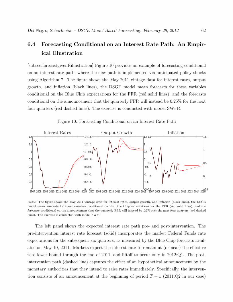
Del Negro, Schorfheide – DSGE Model Based Forecasting: February 29, 2012 62
6.4 Forecasting Conditional on an Interest Rate Path: An Empir-
ical Illustration
[subsec:forecastgivenRillustration] Figure 10 provides an example of forecasting conditional
on an interest rate path, where the new path is implemented via anticipated policy shocks
using Algorithm 7. The figure shows the May-2011 vintage data for interest rates, output
growth, and inflation (black lines), the DSGE model mean forecasts for these variables
conditional on the Blue Chip expectations for the FFR (red solid lines), and the forecasts
conditional on the announcement that the quarterly FFR will instead be 0.25% for the next
four quarters (red dashed lines). The exercise is conducted with model SWπR.
Figure 10: Forecasting Conditional on an Interest Rate Path
Interest Rates Output Growth Inflation
2007 2008 2009 2010 2011 2012 2013 2014 20150
0.2
0.4
0.6
0.8
1
1.2
1.4
0
0.2
0.4
0.6
0.8
1
1.2
1.4
2007 2008 2009 2010 2011 2012 2013 2014 2015−2
−1.5
−1
−0.5
0
0.5
1
1.5
−2
−1.5
−1
−0.5
0
0.5
1
1.5
2007 2008 2009 2010 2011 2012 2013 2014 2015−0.5
0
0.5
1
1.5
−0.5
0
0.5
1
1.5
Notes: The figure shows the May 2011 vintage data for interest rates, output growth, and inflation (black lines), the DSGE
model mean forecasts for these variables conditional on the Blue Chip expectations for the FFR (red solid lines), and the
forecasts conditional on the announcement that the quarterly FFR will instead be .25% over the next four quarters (red dashed
lines). The exercise is conducted with model SWπ.
The left panel shows the expected interest rate path pre- and post-intervention. The
pre-intervention interest rate forecast (solid) incorporates the market Federal Funds rate
expectations for the subsequent six quarters, as measured by the Blue Chip forecasts avail-
able on May 10, 2011. Markets expect the interest rate to remain at (or near) the effective
zero lower bound through the end of 2011, and liftoff to occur only in 2012:Q1. The post-
intervention path (dashed line) captures the effect of an hypothetical announcement by the
monetary authorities that they intend to raise rates immediately. Specifically, the interven-
tion consists of an announcement at the beginning of period T + 1 (2011:Q2 in our case)

Del Negro, Schorfheide – DSGE Model Based Forecasting: February 29, 2012 63
that the quarterly FFR will be .25% (1% annualized) for the next four quarters (through
2012:Q1). In terms of the model mechanics, such an announcement amounts to a vec-
tor of time T + 1 unanticipated and anticipated shocks computed in such a way to obtain
RT+1 = IET+1[RT+2] = .. = IET+1[RT+4] = 0.25, as described in Algorithm 7.
Consistent with the impulse responses shown in Figure 9, the announcement that policy
will be more contractionary than expected leads to lower inflation and lower output growth.
The effect of the announcement on output growth is front-loaded, as we discussed in Sec-
tion 6.1. On impact (2011:Q2) the difference between the solid and dashed lines is about
75 basis points, that is, roughly 3% annualized. The difference narrows over the following
two quarters and is about zero in 2012:Q1, even though the difference in interest rates in
that quarter is almost as large as it was in 2011:Q2. After 2012:Q1 output growth following
the contractionary announcement is actually higher than otherwise. This is not surprising
in light of the fact that monetary policy is still neutral in this model. Slower growth in the
short-run must be compensated by higher growth later, since eventually the effect of the
announcement on the level of output must be zero. Nonetheless the post-intervention level
of output remains below the pre-intervention level at least through 2015, leading to lower
real marginal costs and lower inflation, as shown in the last panel of Figure 10.
7 Moving Beyond Point Forecasts
[sec:densforecast] Thus far, this paper has focused on point forecasts generated from DSGE
models and on how to improve their accuracy by using external information. For the remain-
der of this paper we will explore other aspects of DSGE model forecasts. First, an important
feature that distinguishes DSGE models from many other time series models, is that DSGE
models attribute macroeconomic fluctuations to orthogonal structural shocks. Thus, the
models can provide decompositions of historical time series as well as the predicted path of
the economy. We illustrate the use of shock decompositions in Section 7.1. Second, the al-
gorithms described in the preceding sections generate draws from the predictive distribution
which, as discussed in Section 3.2, can also be used to obtain interval or density forecasts.
In Section 7.2 we generate real-time density forecasts from the SWπ model as well as the
DSGE model with financial frictions introduced in Section 2.2 and examine the extent to
which the forecasts capture the evolution of output growth and inflation during the 2008-09

Del Negro, Schorfheide – DSGE Model Based Forecasting: February 29, 2012 64
recession. Third, in Section 7.3 we examine more systematically whether DSGE model den-
sity forecasts are well calibrated in the sense that stated probabilities are commensurable
with actual frequencies.
7.1 Shock Decompositions
[subsec:shockdecompositions] DSGE models deliver a structural interpretation for both the
history and the forecasts of macroeconomic time series. Figure 11 displays so-called shock
decompositions for output growth and inflation, that illustrate the contribution of the various
structural shocks to the historical and projected evolution of the two series. Before discussing
the results in detail, we present the algorithm that is used to construct the decomposition.
Algorithm 8. Draws from the Posterior Distribution of a Shock Decomposition.
[algo:shockdecomposition] For j = 1 to nsim, select the j’th draw from the posterior distri-
bution p(θ|Y1:T ) and:
1. Use the simulation smoother (see, for instance, the textbook by Durbin and Koopman
(2001) for a description) to generate a draw S(j)0:T from the distribution p(S
(j)0:T |Y1:T , θ
(j)).
2. For each structural shock i = 1, . . . ,m (which is an element of the vector st):
(a) Compute the sequence of shock innovations ε(j)i,1:T , for instance, by solving s
(j)i,t =
ρ(j)i s
(j)i,t−1 + σ
(j)i ε
(j)i,t for ε
(j)i,t .
(b) Define a new sequence of innovations e1:T (et is of the same dimension as εt)
by setting the i’th element ei,t = ε(j)i,t for t = 1, . . . , T and ei,t ∼ N(0, σ2
i ) for
t = T + 1, . . . , T +H. All other elements of et, t = 1, . . . , T +H, are set equal to
zero.
(c) Starting from s0 = s(j)0 , iterate the state transition equation (33) forward using
the innovations e1:T+H to obtain the sequence S(j)1:T+H .
(d) Use the measurement equation (34) to compute Y(j)1:T+H based on S
(j)1:T+H . �
In practice, researchers sometimes take some or all of the following short-cuts: the
parameter draws θ(j) are replaced by the posterior mean or mode, say θ; draws of the

Del Negro, Schorfheide – DSGE Model Based Forecasting: February 29, 2012 65
Figure 11: Shock Decompositions
Output Growth
2007 2008 2009 2010 2011 2012 2013 2014 2015−3
−2.5
−2
−1.5
−1
−0.5
0
0.5
1
1.5
2
−3
−2.5
−2
−1.5
−1
−0.5
0
0.5
1
1.5
2
Inflation
2007 2008 2009 2010 2011 2012 2013 2014 2015−1.5
−1
−0.5
0
0.5
1
g b µ z λf
λw rm π*
−1.5
−1
−0.5
0
0.5
1
Notes: The shock decompositions for output growth (top) and inflation (bottom) are computed using model SWπ estimated
on the last available vintage (May 2011). The black and red lines represent the data and the forecasts, both in deviation from
the steady state. The colored bars represent the contribution of each shock to the evolution of the variables.

Del Negro, Schorfheide – DSGE Model Based Forecasting: February 29, 2012 66
sequence S(j)0:T are replaced by the mean of the distribution p(S0:T |Y1:T , θ); and future values
of ei,t (Step 2(b)) are set to zero.
The shock decomposition for output growth and inflation in Figure 11 is obtained from
the SWπ model based on the May-2011 data vintage and provides an interpretation of the
2008-09 recession through the lens of a DSGE model. The black and red lines represent
the data and the forecasts, both in deviations from the steady state. The colored bars
represent the contribution of each shock in the model to the evolution of the historical and
the projected path of the two series. The bars in Figure 11 show the posterior mean of
the output generated with Algorithm 8. The two shocks chiefly responsible for the drop in
output (top panel of Figure 11) are shocks that captures imperfections in financial markets,
namely the discount rate (b) and the marginal efficiency of investment (µ) shocks.
As discussed in Smets and Wouters (2007), the discount rate shock has similar effects
as a shock to the external finance premium in a model with explicit financial frictions as in
Section 2.2. This is evident from the no-arbitrage condition (18). All else equal, a negative
b shock coincides with an increase in the expected return of capital. Likewise, an increase
in the riskiness of entrepreneurial projects (positive σω shock) raises the spread between the
expected return on capital and the riskless rate. The µ shock captures, in a broad sense, the
headwinds from the crisis. More precisely, the shock shifts the efficiency with which savings
are turned into future capital, and therefore serves as a proxy for the efficiency of financial
intermediation (see Justiniano, Primiceri, and Tambalotti (2009)).
Wage mark-up (λw) and monetary policy (rm) shocks also play a significant role in
the 2008-09 recession. Wage mark-up shocks capture imperfections in the labor market,
whereas the monetary policy shocks capture unanticipated deviations from the systematic
part of the interest rate feedback rule. During the recession output and inflation were very
low compared to their target value. According to the systematic part of the interest-rate
feedback rule nominal interest rates should have been below zero during this period. Since
the linearized version of the DSGE model ignores the zero-lower-bound constraint on the
nominal interest rate, contractionary monetary policy shocks are necessary to rationalize
the observed 25bp interest rates. The contractionary monetary policy shocks contributed
to the depth of the recession. Finally, positive productivity shocks are the main drivers of
the recovery in GDP after the trough, which is consistent with the behavior of measured
productivity.

Del Negro, Schorfheide – DSGE Model Based Forecasting: February 29, 2012 67
The same shocks that drive fluctuations in economic activity – µ and b shocks – also
explain much of the business-cycle frequency movements in inflation. This is not surprising
in light of the New Keynesian Phillips curve. These shocks depress the level of output, and
therefore real marginal costs, for a long period of time, and consequently lead to inflation
below trend. Productivity shocks also play an important role, as positive shocks lead to
lower real marginal costs, ceteris paribus. High frequency movements in inflation, e.g., due
to oil price shocks, are captured by price mark-up shocks (λf ). Conversely, movements in
the inflation target (π∗), which are disciplined by the use of long-run inflation expectations
in the SWπ model, capture low frequency inflation movements.
Figure 11 is also helpful in explaining the forecasts. For instance, the SWπ model
forecasts above trend output growth throughout the forecast horizon largely because of b
and µ shocks: as the economy recovers from the Great Recession, the negative impact of
these shocks on the level of output diminishes, and this results in a boost in terms of growth
rates. Because of their protracted effect on economic activity, these shocks also keep inflation
lower than steady state.
7.2 Real-Time DSGE Density Forecasts During the Great Reces-
sion: A Post-Mortem
[subsec:densforecastcrisis] After having provided an ex-post rationalization of the 2008-09
recession in the previous section, we now examine ex-ante forecasts of the SWπ model as
well as two variants of the DSGE model with financial frictions discussed in Section 2.2,
henceforth SWπ-FF. Figure 12 shows the DSGE models’ and Blue Chip’s forecasts for output
growth (in Q-o-Q percent) obtained at three different junctures of the financial crisis that
lead to the recession. The dates coincide with Blue Chip forecasts releases: (i) October 10,
2007, right after turmoil in financial markets had begun in August of that year; (ii) July 10,
2008, right before the default of Lehman Brothers; and (iii) January 10, 2009, at or near the
apex of the crisis. Specifically, each panel shows the current real GDP growth vintage (black
line), the DSGE model’s mean forecasts (red line) and percentile bands of the predictive
distribution (shaded blue areas indicate 50% (dark blue), 60%, 70%, 80%, and 90% (light
blue) bands), the Blue Chip forecasts (blue diamonds), and finally the actual realizations
according to the May-2011 vintage (black dashed line).

Del Negro, Schorfheide – DSGE Model Based Forecasting: February 29, 2012 68
In interpreting the results, the reader should bear in mind that the information used
to generate the forecasts depicted in Figure 12 consists only of data that was available at
the beginning of October 2007, July 2008, and January 2009, respectively. For instance, by
January 10, 2009 the forecaster would have access to NIPA samples that end in 2008:Q3 data.
The information set of the Blue Chip forecasters, on the other hand, contains additional
information such as economic indicators for 2008:Q4, information from financial markets,
and a plethora of qualitative information provided by the media, speeches of government
officials, et cetera.
Each row of Figure 12 contains forecasts from a different model. We consider the SWπ
model, the SWπ-FF model, and a specification that we label as SWπ-FF-Current. The two
key differences between the SWπ and the SWπ-FF model are the introduction of financial
frictions as in Bernanke, Gertler, and Gilchrist (1999) and the use of the Baa-10 year Treasury
rate spread as an observable, which arguably captures distress in financial markets.13 The
difference between the SWπ-FF and the SWπ-FF-Current specification is that forecasts
from the latter also utilize the Federal Funds rate and spreads of the most recent quarter,
that is, of the quarter for which NIPA data is not yet available. For instance, the January
2009 SWπ-FF-Current forecast incorporates the average Federal Funds rate and the average
spread for 2008:Q4. At any point in time, the information used to generate predictions from
the SWπ-FF-Current model remains a subset of the information that has been available to
the Blue Chip forecasters.
The October 10, 2007, Blue Chip Consensus forecasts for output are relatively upbeat,
at or above 0.5% Q-o-Q, that is, 2% annualized, as shown in the panels in the first column of
Figure 12. The SWπ forecasts are less optimistic, especially in the short run. The model’s
mean forecasts for output growth are barely above zero in 2008:Q1, with a non-negligible
probability of sustained negative growth (recession) throughout the year. The forecasts for
the two SWπ-FF specifications are in line with those of the SWπ model, although a bit more
subdued. Quarter by quarter, the SWπ-FF specifications assign a probability of 50% or more
to the occurrence of negative growth. While the DSGE models capture the slowdown that
occurred in late 2007 and early 2008, they do not anticipate the subsequent post-Lehman
13Gilchrist and Zakrajsek (forthcoming) use secondary market prices of corporate bonds to construct a
credit spread index that, they argue, is a a considerably more powerful predictor of economic activity than
the measure of spreads we use. Their finding suggests that using an improved measure of spreads may further
improve the SWπ-FF model’s predictive ability.

Del Negro, Schorfheide – DSGE Model Based Forecasting: February 29, 2012 69
Figure 12: Predicting the Crisis: Model and Blue Chip Forecasts for Output Growth
October 10, 2007 (2007Q2 data) July 10, 2008 (2008Q1 data) January 10, 2009 (2008Q3 data)
SWπ Model
2003 2004 2005 2006 2007 2008 2009 2010 2011−2
−1.5
−1
−0.5
0
0.5
1
1.5
2
2.5
3
−2
−1.5
−1
−0.5
0
0.5
1
1.5
2
2.5
3
2004 2005 2006 2007 2008 2009 2010 2011 2012−2
−1.5
−1
−0.5
0
0.5
1
1.5
2
2.5
3
−2
−1.5
−1
−0.5
0
0.5
1
1.5
2
2.5
3
2004 2005 2006 2007 2008 2009 2010 2011 2012−2
−1.5
−1
−0.5
0
0.5
1
1.5
2
2.5
3
−2
−1.5
−1
−0.5
0
0.5
1
1.5
2
2.5
3
SWπ-FF Model
2003 2004 2005 2006 2007 2008 2009 2010 2011−2
−1.5
−1
−0.5
0
0.5
1
1.5
2
2.5
3
−2
−1.5
−1
−0.5
0
0.5
1
1.5
2
2.5
3
2004 2005 2006 2007 2008 2009 2010 2011 2012−2
−1.5
−1
−0.5
0
0.5
1
1.5
2
2.5
3
−2
−1.5
−1
−0.5
0
0.5
1
1.5
2
2.5
3
2004 2005 2006 2007 2008 2009 2010 2011 2012−2
−1.5
−1
−0.5
0
0.5
1
1.5
2
2.5
3
−2
−1.5
−1
−0.5
0
0.5
1
1.5
2
2.5
3
SWπ-FF Model + Current Informaton on FFR and Spreads
2003 2004 2005 2006 2007 2008 2009 2010 2011−2
−1.5
−1
−0.5
0
0.5
1
1.5
2
2.5
3
−2
−1.5
−1
−0.5
0
0.5
1
1.5
2
2.5
3
2004 2005 2006 2007 2008 2009 2010 2011 2012−2
−1.5
−1
−0.5
0
0.5
1
1.5
2
2.5
3
−2
−1.5
−1
−0.5
0
0.5
1
1.5
2
2.5
3
2004 2005 2006 2007 2008 2009 2010 2011 2012−2
−1.5
−1
−0.5
0
0.5
1
1.5
2
2.5
3
−2
−1.5
−1
−0.5
0
0.5
1
1.5
2
2.5
3
Notes: The panels show for each model/vintage the available real GDP growth data (black line), the DSGE model’s mean
forecasts (red line) and bands of its forecast distribution (shaded blue areas; these are the 50, 60, 70, 80, and 90 percent bands,
in decreasing shade), the Blue Chip forecasts (blue diamonds), and finally the actual realizations according to the last available
vintage (May 2011, black dashed line) . All the data are in percent, Q-o-Q.

Del Negro, Schorfheide – DSGE Model Based Forecasting: February 29, 2012 70
collapse of economic activity. The decline in real GDP that occurred in 2008:Q4 lies far in the
tails of the predictive distribution generated by the SWπ model. While the DSGE models
with financial frictions place more probability on growth rates below -1% than the SWπ
model, the 2008:Q4 growth rate still falls outside of the 90% credible prediction intervals.
In July 2008 the Blue Chip forecast and the mean forecast for the SWπ model are roughly
aligned. Both foresaw a weak economy – but not negative growth – in 2008, and a rebound
in 2009. The two SWπ-FF specifications are less sanguine. Their forecasts for 2008 are only
slightly more pessimistic than the Blue Chip forecast for 2008, but, unlike Blue Chip, the
financial frictions models do not predict a strong rebound of the economy in 2009. While
the two SWπ-FF deliver point forecasts of essentially zero growth in 2008:Q4, the models
assign a lot of probability to strongly negative growth rates. As a consequence, the realized
-1.7% growth rate in the last quarter of 2008 falls almost within the 90% credible interval
associated with the predictive distribution.
By January 2009 the scenario has changed dramatically: Lehman Brothers has filed for
bankruptcy a few months earlier (September 15, 2008), stock prices have fallen, financial
markets are in disarray, and various current indicators have provided evidence that real
activity was tumbling. None of this information was available to the SWπ model, which for
the January 10, 2009 forecast round uses data up to 2008:Q3. Not surprisingly, the model
is out of touch with reality with regard to the path of economic activity in 2008:Q4 and
thereafter. It predicts a positive growth rate of 0.5% for the fourth quarter, while the actual
growth rate is approximately -1.7%. The SWπ-FF model is less optimistic, it forecasts zero
growth for 2008:Q4, but also misses the steep decline. The SWπ-FF uses spreads as an
observable, but since the Lehman bankruptcy occurred toward the end of the third quarter,
it had minor effects on the average Baa-10 year Treasury rate spread for 2008:Q3. As a
consequence, the SWπ-FF model has little direct information on the turmoil in financial
markets.
Finally, we turn to the forecasts from the SWπ-FF-Current specification, which uses
2008:Q4 observations on spreads and the Federal Funds rate. This model produces about
the same forecast as Blue Chip for 2008:Q4. Unlike Blue Chip forecasters, the agents in the
laboratory DSGE economy have not seen the Fed Chairman and the Treasury Secretary on
television painting a dramatically bleak picture of the U.S. economy. Thus, we regard it as a
significant achievement that the DSGE model forecasts and the Blue Chip forecasts are both

Del Negro, Schorfheide – DSGE Model Based Forecasting: February 29, 2012 71
Figure 13: Predicting the Crisis: Model and Blue Chip Forecasts for Inflation
October 10, 2007 (2007Q2 data) July 10, 2008 (2008Q1 data) January 10, 2009 (2008Q3 data)
SWπ Model
2003 2004 2005 2006 2007 2008 2009 2010 2011−0.5
0
0.5
1
1.5
−0.5
0
0.5
1
1.5
2004 2005 2006 2007 2008 2009 2010 2011 2012−0.5
0
0.5
1
1.5
−0.5
0
0.5
1
1.5
2004 2005 2006 2007 2008 2009 2010 2011 2012−0.5
0
0.5
1
1.5
−0.5
0
0.5
1
1.5
SWπ-FF Model
2003 2004 2005 2006 2007 2008 2009 2010 2011−0.5
0
0.5
1
1.5
−0.5
0
0.5
1
1.5
2004 2005 2006 2007 2008 2009 2010 2011 2012−0.5
0
0.5
1
1.5
−0.5
0
0.5
1
1.5
2004 2005 2006 2007 2008 2009 2010 2011 2012−0.5
0
0.5
1
1.5
−0.5
0
0.5
1
1.5
SWπ-FF Model + Current Informaton on FFR and Spreads
2003 2004 2005 2006 2007 2008 2009 2010 2011−0.5
0
0.5
1
1.5
−0.5
0
0.5
1
1.5
2004 2005 2006 2007 2008 2009 2010 2011 2012−0.5
0
0.5
1
1.5
−0.5
0
0.5
1
1.5
2004 2005 2006 2007 2008 2009 2010 2011 2012−1
−0.5
0
0.5
1
1.5
−1
−0.5
0
0.5
1
1.5
Notes: The panels show for each model/vintage the available GDP deflator data (black line), the DSGE model’s mean forecasts
(red line) and bands of its forecast distribution (shaded blue areas; these are the 50, 60, 70, 80, and 90 percent bands, in
decreasing shade), the Blue Chip forecasts (blue diamonds), and finally the actual realizations according to the last available
vintage (May 2011, black dashed line) . All the data are in percent, Q-o-Q.

Del Negro, Schorfheide – DSGE Model Based Forecasting: February 29, 2012 72
around -1.3%. More importantly, we find this to be convincing evidence on the importance
of using appropriate information in forecasting with structural models.
Figure 13 conducts the same post-mortem for inflation. On October 10, 2010, all three
specifications generate similar forecasts of inflation. The mean quarterly forecasts are above
0.5% (2% annualized) in 2007, and slightly below 0.5% throughout the rest of the forecast
horizon. Blue Chip forecasts are more subdued for 2007, and correctly so, but essentially
coincide with the DSGE models’ forecasts thereafter. The DSGE model point forecasts
overstate inflation in 2009 and 2010. As the structural models miss the severity of the Great
Recession, they also miss its impact on the dynamics of prices. In terms of density forecasts
however, the forecasts of inflation are not as bad as those for output: In 2009 and 2010 the
ex-post realizations of inflation are mostly within the 70 and 50% bands, respectively.
The July 10, 2008, Blue Chip forecasts for inflation increase quite a bit compared to
2007. The U.S. economy has just been hit by a commodity shock and, moreover, the Federal
Reserve has lowered rates in response to the financial crisis, leading to Blue Chip quarterly
inflation forecasts above 0.5% (2% annualized) throughout the forecast horizon. The mean
DSGE model forecasts are instead slightly more subdued than in 2007, especially for the
models with financial frictions. This occurs for two reasons. First, the DSGE models have no
information on the recent rise in commodity prices. Second, the models perceive a weakness
in aggregate activity and translate that into a moderate inflation outlook.
By 2008:Q3 inflation has risen following the commodity shock. Nonetheless, the January
10, 2009, inflation forecasts of the DSGE models are low. While all three models correctly
assume the high 2008Q3 inflation to be temporary, there exist significant differences in the
inflation forecasts across models, which reflect their different assessment of the state of the
economy. The SWπ and SWπ-FF models’ mean forcasts for inflation are generally above
the actuals for 2009 and 2010. Blue Chip consensus forecasts are – correctly – more subdued
than these forecasts for 2008:Q4 and the first half of 2009, but are no different afterwards:
quarterly inflation quickly reverts to 0.5% in their outlook. Conversely, the SWπ-FF-current
model predicts inflation to remain low throughout the forecast horizon, which is consistent
with the actual evolution of this variable in the aftermath of the Great Recession.
The examination of DSGE model forecasts during the 2008-09 recession suggests that
the DSGE models with financial frictions are preferable to the SWπ model. It turns out
that this ranking is not stable over time. Figure 14 depicts RMSE differentials for the SWπ

Del Negro, Schorfheide – DSGE Model Based Forecasting: February 29, 2012 73
Figure 14: Difference in Forecasting Accuracy Over Time: SWπ and SWπFF-Current
Difference in 4-quarter-ahead Rolling RMSEsOutput Inflation
1992 1994 1996 1998 2000 2002 2004 2006 2008 2010 2012−0.5
−0.4
−0.3
−0.2
−0.1
0
0.1
0.2
1992 1994 1996 1998 2000 2002 2004 2006 2008 2010 2012−0.1
−0.08
−0.06
−0.04
−0.02
0
0.02
0.04
0.06
0.08
Notes: The figure shows the difference over time in 4-quarter-ahead rolling RMSEs between the SWπ and SWπFF-Current
models for output growth and inflation. At each point in time, the RMSEs are computed using the previous 12 quarters, that
is, the figure shows RMSEt(SWπ)−RMSEt(SWπFF-Current), where RMSEt(Mi) =
r112
P11j=0
“yt−j − y
Mit−j|t−j−4
”2and
yMit−j|t−j−4
is the 4-quarter ahead forecast of yt−j obtained using model Mi, Mi = {SWπ, SWπFF-Current}.
model and the SWπ-FF-Current model for h = 4-step-ahead forecasts (the results for model
SWπ-FF are very similar). At each point in term the RMSEs are computed using the 12
previous quarters. A value greater than zero indicates that the financial-frictions model
attains a lower RMSE. The Figure indicates that on average over the forecast period the
model without financial frictions generates more accurate forecasts. However, during the
recent financial crisis, the ordering is reversed. The SWπ-FF-Current model contains an
additional mechanism that associates high spreads with low economic activity and helps the
model to track and forecast aggregate output and inflation throughout the crisis.
7.3 Calibration of Density Forecasts
[subsec:densforecastcalibration] We previously presented a variety of interval and density
forecasts which begs the question of how accurate these forecasts are. While, strictly speak-

Del Negro, Schorfheide – DSGE Model Based Forecasting: February 29, 2012 74
ing, predictive distributions in a Bayesian framework are subjective, the statistics reported
below provide a measure of the extent to which the predicted probabilities of events are
consistent with their observed frequencies. Dawid (1984) views this consistency as a min-
imal desirable property for probability forecasts. Bayarri and Berger (2004) refer to the
notion that in repeated practical use of a sequential forecasting procedure the long-run av-
erage level of accuracy should be consistent with the long-run average reported accuracy as
frequentist principle. The literature, see for instance Dawid (1982), refers to sequences of
(subjective) density forecasts that adhere to the frequentist principle as well calibrated. To
assess whether DSGE model density forecasts are well calibrated we generate histograms for
probability integral transformations (PITs).
Starting with Dawid (1984) and Kling and Bessler (1989) the use of probability inte-
gral transformations (PITs) has a fairly long tradition in the literature on density forecast
evaluation. The PIT of yi,T+h based on its time T predictive distribution as
zi,h,T =
∫ yi,T+h
−∞p(yi,T+h|Y1:T )dyi,T+h. (73)
Thus, the PIT is defined as the cumulative density of the random variable yi,T+h evaluated at
yi,T+h. Based on the output of Algorithm 2 the PITs can be easily approximated by (recall
that I{x ≥ a} denotes the indicator function)
zi,h,T ≈nsim∑j=1
I{y(j)i,T+h ≤ yi,T+h},
where yi,T+h is now the value of yi observed in period T+h. It is straightforward to show that
the marginal distribution of PITs is uniform. Consider a random variable X with density
F (x). Then
P{F (X) ≤ z} = P{X ≤ F−1(z)} = F(F−1(z)
)= z
Building on results by Rosenblatt (1952), Diebold, Gunther, and Tay (1998) show that for
h = 1 the zi,t,h’s are not just uniformly distributed, but they are also independent across
time: zi,t,h ∼ iid U [0, 1]. For this reason, PITs are often called generalized residuals.
Below, we plot PIT histograms and informally assess the distance of the unconditional
empirical distribution of the PITs from the uniform distribution. A more formal assess-

Del Negro, Schorfheide – DSGE Model Based Forecasting: February 29, 2012 75
ment, via posterior predictive checks, is provided in Herbst and Schorfheide (2011).14 It
is important to stress that the uniformity of PITs does not imply that a forecast is sharp.
Abstracting from parameter uncertainty, suppose that yt evolves according to
yt = θyt−1 + ut, ut ∼ iidN(0, 1), 0 ≤ θ < 1. (74)
Moreover, suppose that Forecaster F1 reports the predictive density N(θyt−1, 1), whereas
forecaster F2 reports the density forecast N(0, 1/(1− θ2)
). Both forecasts lead to PITs that
are unconditionally uniformly distributed. The uniformity of the PITs associated with F2
follows immediately. Let Φ(·) denote the cdf of a N(0, 1) random variable. For F1 it can be
verified as follows:
P(yt,yt−1){Φ(yt − θyt−1) ≤ z
}= Eyt−1
[Pyt
yt−1
{Φ(yt − θyt−1) ≤ z
}]= Eyt−1 [z] = z.
The unconditional probability needs to be computed under the joint distribution of (yt, yt−1).
It can be obtained by first conditioning on yt−1 and subsequently integrating out yt−1, which
leads to the first equality. The second equality follows from (74). However, as long as
θ > 0, F1’s forecast will be more precise than F2’s forecast because it exploits conditioning
information that reduces the variance of the predictive distribution from 1/(1− θ2) to 1. In
fact, conditional on yt−1 the cdf of the PIT computed from F2 is given by
Pytyt−1
{Φ(√
1− θ2yt
)≤ z
}= Φ
(Φ−1(z)√
1− θ− θyt−1
),
which implies that the sequence of PITs from F2 is not independently distributed.
As we have seen in Section 5, DSGE model forecasts often do not exploit all the available
information and therefore might not be as sharp as other forecasts. Nonetheless, it remains
interesting to assess whether the predictive distributions are well-calibrated in the sense that
PITs have an unconditional distribution that is approximately uniform. Figure 15 depicts
14As emphasized by Geweke and Whiteman (2006), Bayesian approaches to forecast evaluation are funda-
mentally different from frequentist approaches. In a Bayesian framework there is no uncertainty about the
predictive density given the specified collection of models, because predictive densities are simply constructed
by the relevant conditioning. Non-Bayesian approaches, see Corradi and Swanson (2006), tend to adopt the
notion of a “true” data-generating process (DGP) and try to approximate the predictive density inherent in
the DGP with a member of a collection of probability distributions indexed by a parameter θ. To the extent
that the forecaster faces uncertainty with respect to θ, there is uncertainty about the density forecast itself,
and non-Bayesian assessments try to account for this uncertainty.

Del Negro, Schorfheide – DSGE Model Based Forecasting: February 29, 2012 76
Figure 15: PITs: SWπ model
2 Quarters-AheadOutput Growth Inflation Interest Rates
0 0.2 0.4 0.6 0.8 10
5
10
15
20
25
30
35
40
45
50
0 0.2 0.4 0.6 0.8 10
5
10
15
20
25
30
35
40
45
50
0 0.2 0.4 0.6 0.8 10
5
10
15
20
25
30
35
40
45
50
4 Quarters-AheadOutput Growth Inflation Interest Rates
0 0.2 0.4 0.6 0.8 10
5
10
15
20
25
30
35
40
45
50
0 0.2 0.4 0.6 0.8 10
5
10
15
20
25
30
35
40
45
50
0 0.2 0.4 0.6 0.8 10
5
10
15
20
25
30
35
40
45
50
8 Quarters-AheadOutput Growth Inflation Interest Rates
0 0.2 0.4 0.6 0.8 10
5
10
15
20
25
30
35
40
45
50
0 0.2 0.4 0.6 0.8 10
5
10
15
20
25
30
35
40
45
50
0 0.2 0.4 0.6 0.8 10
5
10
15
20
25
30
35
40
45
50
Notes:
histograms for PITs based on forecasts generated with the SWπ model. We group the PITs
into five equally sized bin. Under a uniform distribution, each bin should contain 20% of
the PITs, indicated by the solid horizontal lines in the figure. The empirical distribution
looks quite different from a uniform distribution and the discrepancy increases with forecast
horizon h. For output growth, an overly large fraction of PITs fall into the 0.4-0.6 bin. This
indicates that the predictive distribution is too diffuse.

Del Negro, Schorfheide – DSGE Model Based Forecasting: February 29, 2012 77
One potential explanation is that all of the forecasts are generated post 1984 and most
of them fall into the period of the so-called Great Moderation. The estimation sample,
on the other hand, contains a significant fraction of observations from the pre-1984 period.
Thus, the shock standard deviations, roughly speaking, are estimated to capture an average
of the pre- and post-moderation volatility, which means that they tend to overpredict the
volatility during the forecast period. While the empirical distribution of the output growth
PITs is essentially symmetric, the PITs associated with inflation and interest rate forecasts
have a slightly skewed distribution. The DSGE model assigns substantial probability to low
inflation rates that never materialize. Vice versa, the model also assigns positive probability
to relatively high interest rates that are not observed during the forecast period. Further
results on the evaluation of density forecasts of medium-scale DSGE models can be found in
Herbst and Schorfheide (2011) and Wolters (2010).
8 Conclusion and Outlook
[sec:conclusion] This paper reviewed the recent literature on forecasting with DSGE models,
discussed numerous useful algorithms, and provided empirical illustrations of the various
methods considered. We presented some novel methods that allow modelers to incorporate
external information and that may increase the accuracy of DSGE model forecasts. More-
over, we compared methods of generating forecasts conditional on desired interest rate paths,
and studied the forecasting performance of DSGE models with and without financial frictions
during the 2008-09 recession. In closing, we provide some discussion of why we think that
DSGE-model-based forecasts are useful, we review empirical approaches that relax some of
the DSGE model-implied restrictions to improve forecast accuracy, and lastly we engage in
a wild speculation about the future of DSGE model forecasting.
8.1 Why DSGE Model Forecasting?
A macroeconomic forecaster can in principle choose from a large pool of econometric models.
Some models are univariate, others are multivariate; some are linear, others are nonlinear;
some are based on economic theory whereas others simply exploit correlations in the data.
Empirical DSGE models are multivariate, in most instances they are linearized, and they

Del Negro, Schorfheide – DSGE Model Based Forecasting: February 29, 2012 78
build upon modern dynamic macroeconomic theory which emphasizes intertemporal decision
making and the role of expectations. The benefit of building empirical models on sound
theoretical foundations is that the model delivers an internally consistent interpretation of
the current state and future trajectories of the economy and enables a sound analysis of policy
scenarios. The potential cost is that theory-implied cross-coefficient restrictions might lead
to a deterioration in forecast performance.
While a decade ago the costs outweighed the benefits, the scale has tipped in favor of
DSGE models in recent years. First, DSGE models have been enriched with endogenous
propagation mechanisms, e.g. Christiano, Eichenbaum, and Evans (2005), and exogenous
propagation mechanisms, e.g. Smets and Wouters (2003, 2007), which allow the models
to better capture the autocovariance patterns in the data. Second, as demonstrated in
Section 5, DSGE models can be easily modified to incorporate external information into
the forecasts, both real-time information about the current state of the economy as well
information about its long run trends. Real-time information is interpreted by the models
as information about the realization of the structural shocks, and is useful to improve the
accuracy of short-horizon forecasts. Moreover, long-run inflation expectations can be used
to anchor long-horizon forecasts of nominal variables.
The case for DSGE model forecasting ultimately rests on the fact that these models pro-
vide a good package. Granted, there exist time series models that generate more accurate
univariate forecasts of output growth and inflation, but these models might miss comove-
ments between these two variables. Bayesian VARs tend to be good multivariate forecasting
models but it is difficult to identify more than one or two structural shocks and to provide a
narrative for the current and future state of the economy. Moreover, VARs typically do not
have enough structure to generate predictions about anticipated changes in interest rates.
Dynamic factor models are able to extract information from a large cross section of macroe-
conomic variables and to explain the comovements among these series as being generated by
a low-dimensional vector of latent variables. While the forecasting record of these models is
strong, the policy experiments that could be carried out with these models are very limited.
Finally, none of the aforementioned models would allow the user to measure the degree of
distortion in the economy that ought to be corrected through monetary policy.
Estimated DSGE models can perform a lot of tasks simultaneously. They generate
multivariate density forecasts that reflect parameter and shock uncertainty. They provide a

Del Negro, Schorfheide – DSGE Model Based Forecasting: February 29, 2012 79
device of interpreting the current state and the future path of the economy through the lens of
modern dynamic macroeconomics and provide decompositions in terms of structural shocks.
Moreover, the models enable the user to generate predictions of the effect of alternative
policy scenarios. While a successful decathlete may not be the fastest runner or the best
hammer thrower, she certainly is a well-rounded athlete.
8.2 Beyond DSGE Models
Throughout this paper have focused on forecasts generated from specific DSGE models.
In closing we briefly mention some strands of the literature that either relax some of the
DSGE model restrictions to improve their forecast performance or combine different classes
of econometric models. Ingram and Whiteman (1994) were the first to use DSGE models
to construct a prior distribution for vector autoregressions that is centered at the DSGE
model-implied parameter restrictions. This approach has the advantage that the DSGE
model restrictions are imposed in a non-dogmatic manner, allowing for modest violations of
the DSGE model restrictions. Del Negro and Schorfheide (2004) developed this approach
further and constructed a hierarchical Bayes model, called DSGE-VAR, that takes the form
of a structural VAR and allows the researcher to simultaneously estimate the parameters
of the DSGE model and the VAR. A hyperparameter determines the scale of the prior
covariance matrix. If the prior covariance matrix is zero, then the DSGE model restrictions
are dogmatically imposed on the VAR.
In the context of a small-scale DSGE model Del Negro and Schorfheide (2004) document
that the best forecasting performance is obtained for an intermediate value of the hyperpa-
rameter that implies that prior distribution and likelihood of the VAR are about equally
informative about the parameters. The DSGE-VAR produces substantially more accurate
pseudo-out-of-sample forecasts than the underlying DSGE model. A similar empirical re-
sult is reported in Del Negro, Schorfheide, Smets, and Wouters (2007) for a variant of the
Smets-Wouters model.15
15Kolasa, Rubaszek, and Skrzypczynski (2010) provide a less favorable assessment of the DSGE-VAR
approach, however. Using the Smets and Wouters (2007) model to generate a prior distribution, the authors
found that the DSGE model actually outperforms the DSGE-VAR. This result might be due to the fact that
the 2007-version of the Smets-Wouters model contains a number of features that are designed to boost its
forecast performance. Also, the DSGE-VAR specification that they use is in first differences.

Del Negro, Schorfheide – DSGE Model Based Forecasting: February 29, 2012 80
An alternative way of combining VARs and DSGE models for macroeconomic forecast-
ing applications is explored by Amisano and Geweke (2011). The authors consider a pool of
macroeconomic models that incorporates, among others, DSGE models and VARs. A com-
bined forecast is generated from a convex combination of the predictive densities associated
with the models included in the pool. The weights are estimated such that asymptotically
the Kullback-Leibler discrepancy between the convex combination of models and some un-
derlying “data generating process” is minimized. The authors find that while the DSGE
model receives a non-trivial weight in the model mixture, the forecasting performance of the
pool is substantially better than the forecasting performance of any of the individual models
in the pool. Waggoner and Zha (2010) extend the Amisano-Geweke approach by allowing
for time-varying model weights that follow a regime-switching process. Moreover, model
parameters and mixture weights are estimated simultaneously rather than sequentially. The
authors identify episodes in which the DSGE model is useful for macroeconomic forecasting
and episodes in which the combined forecasts are dominated by the VAR. The same ap-
proach could be used to combine different DSGE models. As documented in Section 7.2,
the relative ranking of DSGE models without and with financial frictions seems to shift over
time.
Finally, there is a strand of literature that combines DSGE models and dynamic factor
models (DFM). The goal of this literature is to link the DSGE model with a large cross section
of macroeconomic indicators rather than a small set of seven or eight observables as was done
in this paper. One the one hand, the large set of macroeconomic variables might provide
sharper inference about the current state of the economy. On the other hand, this framework
allows the modeler to assess the effect of structural shocks, e.g. monetary policy shocks,
on variables that are not explicitly modeled in the DSGE model. The resulting empirical
specification is called DSGE-DFM. It is essentially a DFM in which the latent factors are
equated with the state variables of a DSGE model and follow the DSGE model-implied law
of motion. The DSGE-DFM was first developed by Boivin and Giannoni (2006) and studied
further by Kryshko (2010) who documents that the space spanned by the factors of a DSGE-
DFM is very similar to the space spanned by factors extracted from an unrestricted DFM.
Schorfheide, Sill, and Kryshko (2010) used a DSGE-DFM to generate DSGE-model-based
forecasts for variables that do not explicitly appear in the DSGE model.

Del Negro, Schorfheide – DSGE Model Based Forecasting: February 29, 2012 81
8.3 The Future
While the literature on forecasting with DSGE models was practically non-existent a decade
ago, it has become a vibrant area of research. A lot of progress has been made in the specifica-
tion of DSGE models, as well as in the development of methods that enable the incorporation
of real-time information, the relaxation of overly tight cross-equation restrictions, and the
combination of DSGE models with other macroeconometric models. The progress is in part
driven by the desire of central banks to incorporate modern macroeconomic equilibrium into
their decision making process. In this regard, the recent crisis with the emergence of noncon-
ventional monetary policies and interest rates near the zero-lower bound has supplied new
challenges for DSGE model-based forecasting that need to be tackled in future research.
References
Adolfson, M., M. K. Andersson, J. Linde, M. Villani, and A. Vredin (2007):
“Modern Forecasting Models in Action: Improving Macroeconomic Analyses at Central
Banks,” International Journal of Central Banking, 3(4), 111–144.
Adolfson, M., J. Linde, and M. Villani (2007): “Forecasting Performance of an Open
Economy Dynamic Stochastic General Equilibrium Model,” Econometric Reviews, 26(2-4),
289–328.
Amisano, G., and J. Geweke (2011): “Prediction with Macroeconomic Models,”
Manuscript.
An, S., and F. Schorfheide (2007a): “Bayesian Analysis of DSGE Models,” Econometric
Reviews, 26(2-4), 113–172.
(2007b): “Bayesian Analysis of DSGE Models–Rejoinder,” Econometric Reviews,
26(2-4), 211–219.
Aruoba, S. B., and F. Schorfheide (2010): “Sticky Prices versus Monetary Frictions:
An Estimation of Policy Trade-offs,” American Economic Journal: Macroeconomics, forth-
coming.

Del Negro, Schorfheide – DSGE Model Based Forecasting: February 29, 2012 82
Bayarri, M., and J. Berger (2004): “The Interplay of Bayesian and Frequentist Analy-
sis,” Statistical Science, 19(1), 58–80.
Benes, J., A. Binning, and K. Lees (2008): “Incorporating judgement with DSGE
models,” Manuscript, DP2008/10.
Bernanke, B., M. Gertler, and S. Gilchrist (1999): “The Financial Accelerator in
a Quantitative Business Cycle Framework,” in Handbook of Macroeconomics, ed. by J. B.
Taylor, and M. Woodford, vol. 1C. North Holland, Amsterdam.
Blake, A. (2011): “Fixed Interest Rates over Finite Horizons,” Bank of England Working
Paper, No. 808.
Boivin, J., and M. P. Giannoni (2006): “DSGE Models in a Data Rich Enviroment,”
NBER Working Paper, 12772.
Carlstrom, C., T. Fuerst, and M. Paustian (2012): “How Inflationary Is an Extended
Period of Low Interest Rates,” Manuscript.
Carter, C., and R. Kohn (1994): “On Gibbs Sampling for State Space Models,”
Biometrika, 81(3), 541–553.
Chib, S., and S. Ramamurthy (2010): “Tailored Randomized Block MCMC Methods
with Application to DSGE Models,” Journal of Econometrics, 155(1), 19–38.
Christiano, L., R. Motto, and M. Rostagno (2009): “Financial Factors in Economic
Fluctuations,” Manuscript, Northwestern University and European Central Bank.
Christiano, L. J., M. Eichenbaum, and C. L. Evans (2005): “Nominal Rigidities
and the Dynamic Effects of a Shock to Monetary Policy,” Journal of Political Economy,
113(1), 1–45.
Christoffel, K., G. Coenen, and A. Warne (2010): “Forecasting with DSGE Models,”
in Oxford Handbook on Economic Forecasting, ed. by M. Clements, and D. Hendry, p.
forthcoming. Oxford University Press.
Coenen, G., P. McAdam, and R. Straub (2008): “Tax Reform and Labor Market
Performance in the Euro Area: A Simulation-based Analysis Using the New Area-Wide
Model,” Journal of Economic Dynamics and Control, 32(8), 2543–2583.

Del Negro, Schorfheide – DSGE Model Based Forecasting: February 29, 2012 83
Corradi, V., and N. Swanson (2006): “Predictive Density Evaluation,” in Handbook
of Economic Forecasting, ed. by G. Elliott, C. Granger, and A. Timmermann, vol. 1 of
Handbooks in Economics 24, pp. 197–286. North Holland, Amsterdam.
Dawid, A. (1982): “The Well-Calibrated Bayesian,” Journal of the American Statistical
Association, 77(379), 605–610.
Dawid, A. (1984): “Statistical Theory: The Prequential Approach,” Journal of the Royal
Statistical Society, Series A, 147(2), 278–292.
DeJong, D. N., B. F. Ingram, and C. H. Whiteman (2000): “A Bayesian Approach
to Dynamic Macroeconomics,” Journal of Econometrics, 98(2), 203 – 223.
Del Negro, M., and S. Eusepi (2011): “Fitting Observed Ination Expectations,” Journal
of Economic Dynamics and Control, 35, 2105–2131.
Del Negro, M., and F. Schorfheide (2004): “Priors from General Equilibrium Models
for VARs,” International Economic Review, 45(2), 643 – 673.
(2008): “Forming Priors for DSGE Models (and How it Affects the Assessment of
Nominal Rigidities),” Journal of Monetary Economics, 55(7), 1191–1208.
(2010): “Bayesian Macroeconometrics,” in Handbook of Bayesian Econometrics,
ed. by H. K. van Dijk, G. Koop, and J. Geweke. Oxford University Press.
Del Negro, M., F. Schorfheide, F. Smets, and R. Wouters (2007): “On the Fit
of New Keynesian Models,” Journal of Business and Economic Statistics, 25(2), 123–162.
Diebold, F., T. Gunther, and A. Tay (1998): “Evaluating Density Forecasts with
Applications to Financial Risk Management,” International Economic Review, 39(4), 863–
883.
Doan, T., R. Litterman, and C. A. Sims (1984): “Forecasting and Conditional Pro-
jections Using Realistic Prior Distributions,” Econometric Reviews, 3(4), 1–100.
Durbin, J., and S. J. Koopman (2001): Time Series Analysis by State Space Methods.
Oxford University Press.

Del Negro, Schorfheide – DSGE Model Based Forecasting: February 29, 2012 84
Edge, R., and R. Gurkaynak (2010): “How Useful Are Estimated DSGE Model Fore-
casts for Central Bankers,” Brookings Papers of Economic Activity, p. forthcoming.
Edge, R., M. Kiley, and J.-P. Laforte (2009): “A Comparison of Forecast Performance
Between Federal Reserve Staff Forecasts, Simple Reduced-Form Models, and a DSGE
Model,” Federal Reserve Board of Governors Finance and Economics Discussion Paper
Series, 2009-10.
Erceg, C. J., and A. T. Levin (2003): “Imperfect Credibility and Inflation Persistence,”
Journal of Monetary Economics, 50, 915–944.
Eusepi, S., and E. Monch (2011): “Treasury Term Premia in a Survey-Based Expecta-
tions Hypothesis Model,” Manuscript, FRB New York.
Faust, J., and J. Wright (2011): “Forecasting Inflation,” in Handbook of Economic
Forecasting, ed. by G. Elliott, and A. Timmermann, vol. 2. Elsevier.
Geweke, J., and C. Whiteman (2006): “Bayesian Forecasting,” in Handbook of Economic
Forecasting, ed. by G. Elliott, C. Granger, and A. Timmermann, vol. 1 of Handbooks in
Economics 24, pp. 3–80. North Holland, Amsterdam.
Giannone, D., F. Monti, and L. Reichlin (2009): “Incorporating Conjunctural Analy-
sis in Structural Models,” The Science and Practice of Monetary Policy Today, pp. 41–57.
Gilchrist, S., and E. Zakrajsek (forthcoming): “Credit Spreads and Business Cycle
Fluctuations,” American Economic Review.
Graeve, F. D., M. Emiris, and R. Wouters (2009): “A Structural Decomposition of
the US Yield Curve,” Journal of Monetary Economics, 56(4), 545 – 559.
Greenwood, J., Z. Hercovitz, and P. Krusell (1998): “Long-Run Implications of
Investment-Specific Technological Change,” American Economic Review, 87(3), 342–36.
Herbst, E. (2010): “Gradient and Hessian-based MCMC for DSGE Models,” Manuscript.
Herbst, E., and F. Schorfheide (2011): “Evaluating DSGE Model Forecasts of Co-
movements,” Manuscript, University of Pennsylvania.
Del Negro, Schorfheide – DSGE Model Based Forecasting: February 29, 2012 85
Ingram, B., and C. Whiteman (1994): “Supplanting the Minnesota Prior- Forecasting
Macroeconomic Time Series Using Real Business Cycle Model Priors,” Journal of Mone-
tary Economics, 49(4), 1131–1159.
Justiniano, A., G. E. Primiceri, and A. Tambalotti (2009): “Investment Shocks and
Business Cycles,” NBER Working Paper, 15570.
King, R. G., C. I. Plosser, and S. Rebelo (1988): “Production, Growth, and Business
Cycles: I The Basic Neoclassical Model,” Journal of Monetary Economics, 21(2-3), 195–
232.
Kling, J., and D. Bessler (1989): “Calibration-Based Predictive Distributions: An Ap-
plication of Prequential Analysis to Interest Rates, Money, Prices, and Output,” Journal
of Business, 62(4), 447–499.
Kohn, R., P. Giordani, and I. Strid (2010): “Adaptive Hybrid Metropolis-Hastings
Samplers for DSGE Models,” Riksbank Manuscript.
Kolasa, M., M. Rubaszek, and P. Skrzypczynski (2010): “Putting the New Keyne-
sian DSGE Model to the Real-Time Forecasting Test,” Working Paper.
Kryshko, M. (2010): “Data-Rich DSGE and Dynamic Factor Models,” Manuscript, Uni-
versity of Pennsylvania.
Laseen, S., and L. E. Svensson (2011): “Anticipated Alternative Policy-Rate Paths in
Policy Simulations,” International Journal of Central Banking, 7(3), 1–35.
Leeper, E. M., and T. Zha (2003): “Modest Policy Interventions,” Journal of Monetary
Economics, 50(8), 1673 – 1700.
Milani, F., and J. Treadwell (2011): “The Effects of Monetary Policy ”News” and
”Surprises”,” Manuscript.
Monti, F. (2010): “Combining Judgment and Models,” Journal of Money, Credit and
Banking, 42(8), 1641–1662.
Otrok, C. (2001): “On Measuring the Welfare Costs of Business Cycles,” Journal of
Monetary Economics, 45(1), 61–92.

Del Negro, Schorfheide – DSGE Model Based Forecasting: February 29, 2012 86
Owen, A. B. (2001): Empirical Likelihood. Chapman & Hall / CRC.
Robertson, J. C., E. W. Tallman, and C. H. Whiteman (2005): “Forecasting Using
Relative Entropy,” Journal of Money, Credit, and Banking, 37(3), 383–401.
Rosenblatt, M. (1952): “Remarks on a Multivariate Transformation,” Annals of Mathe-
matical Statistics, 23(3), 470–472.
Rubaszek, M., and P. Skrzypczynski (2008): “On the Forecasting Performance of a
Small-Scale DSGE Model,” International Journal of Forecasting, 24(3), 498–512.
Schorfheide, F. (2000): “Loss Function-Based Evaluation of DSGE Model,” Journal of
Applied Econometrics, 15(6), 645–670.
Schorfheide, F., K. Sill, and M. Kryshko (2010): “DSGE Model-Based Forecasting
of Non-Modelled Variables,” International Journal of Forecasting, 26(2), 348–373.
Silverman, B. (1986): Density Estimation for Statistics and Data Analysis. Chapman &
Hall, New York.
Sims, C. A., and T. Zha (1998): “Bayesian Methods for Dynamic Multivariate Models,”
International Economic Review, 39(4), 949–968.
Smets, F., and R. Wouters (2003): “An Estimated Dynamic Stochastic General Equi-
librium Model of the Euro Area,” Journal of the European Economic Association, 1(5),
1123–1175.
Smets, F., and R. Wouters (2005): “Bayesian New Neoclassical Synthesis (NNS) Models:
Modern Tools for Central Banks,” Journal of the European Economic Association, 3(2-3),
422 – 433.
Smets, F., and R. Wouters (2007): “Shocks and Frictions in US Business Cycles: A
Bayesian DSGE Approach,” American Economic Review, 97(3), 586–606.
Waggoner, D., and T. Zha (1999): “Conditional Forecasts In Dynamic Multivariate
Models,” Review of Economics and Statistics, 81(4), 639–651.
Waggoner, D. F., and T. Zha (2010): “Confronting Model Misspecification in Macroe-
conomics,” Manuscript, Federal Reserve Bank of Atlanta.

Del Negro, Schorfheide – DSGE Model Based Forecasting: February 29, 2012 87
Wieland, V., and M. H. Wolters (2011): “The Diversity of Forecasts from Macroeco-
nomic Models of the US Economy,” Economic Theory, 47, 247–292.
(2012): “Forecasting and Policy Making,” in Handbook of Economic Forecasting,
ed. by G. Elliott, and A. Timmermann, vol. 2. Elsevier.
Wolters, M. H. (2010): “Forecating under Model Uncertainty,” Working Paper.
Wright, J. (2011): “Evaluating Real-Time VAR Forecasts with an Informative Democratic
Prior,” Manuscript.

Del Negro, Schorfheide – DSGE Model Based Forecasting: February 29, 2012 A-1
A Details for Figure 4
Table A-1 lists the RMSEs that are plotted in Figure 4 by study. The specific references for
each study can be found in Table 3.
Table A-2 contains details on the computation of AR(2) forecasts that are used to construct
RMSE ratios.

Del Negro, Schorfheide – DSGE Model Based Forecasting: February 29, 2012 A-2
Table A-1: RMSEs for DSGE and AR(2) Models in Figure 4
h = 1 h = 4
Study Model GDP INFL INT GDP INFL INT
RS DSGE 0.496 0.224 0.130 0.448 0.287 0.335
AR (2) 0.512 0.198 0.083 0.502 0.235 0.320
KRS DSGE 0.485 0.240 0.108 0.477 0.255 0.335
AR (2) 0.471 0.236 0.107 0.465 0.297 0.416
GEW DSGE 0.610 0.290 0.138 0.385 0.350 0.405
AR (2) 0.532 0.221 0.118 0.328 0.281 0.437
W-DS DSGE 0.525 0.262 0.163 0.532 0.272 0.372
AR (2) 0.491 0.257 0.121 0.523 0.331 0.402
W-FM DSGE 0.494 0.321 0.133 0.586 0.330 0.391
AR (2) 0.491 0.257 0.121 0.523 0.331 0.402
W-SW DSGE 0.542 0.255 0.127 0.462 0.279 0.344
AR (2) 0.491 0.257 0.121 0.523 0.331 0.402
W-Edo DSGE 0.529 0.285 0.164 0.511 0.349 0.478
AR (2) 0.491 0.257 0.121 0.523 0.331 0.402
EG DSGE 0.550 0.180 0.110 0.510 0.200 0.100
AR (2) 0.568 0.223 0.122 0.582 0.304 0.425
EKL DSGE 0.448 0.294 0.208 0.502 0.292 0.465
AR (2) 0.626 0.204 0.102 0.734 0.254 0.387
SW DSGE 0.566 0.245 0.108 0.327 0.183 0.354
AR (2) 0.546 0.229 0.126 0.352 0.289 0.467
DSSW DSGE 0.664 0.249 0.123 0.657 0.243 0.394
AR (2) 0.493 0.206 0.111 0.340 0.199 0.357
SSK DSGE 0.510 0.220 0.177 0.410 0.190 0.532
AR (2) 0.525 0.227 0.094 0.469 0.229 0.419

Del Negro, Schorfheide – DSGE Model Based Forecasting: February 29, 2012 A-3
Tab
leA
-2:
ASam
ple
ofStu
die
sR
epor
ting
RM
SE
sfo
rM
ediu
m-S
cale
DSG
EM
odel
s:Par
t1
Stu
dy
Real-ti
me
Act
uals
for
Fore
c.Eval
Act
uals
for
Fore
c.Eval
GD
PD
ata
Fore
cast
Mult
i-
Data
Set?
Use
dfo
rD
SG
EM
odel
Use
dfo
rA
R(2
)M
odel
Per
Capit
a?
Avera
ges?
RS
Yes
One-
year
afte
rth
efo
reca
stin
gor
igin
Fir
stfinal
rele
ase
No
No
KR
SY
esFix
edvin
tage
(200
9:Q
1)Fir
stfinal
rele
ase
No
No
GE
WN
oN
/AFix
edvin
tage
(Jan
2008
)Y
esY
es(O
utp
ut)
W-D
SY
esV
inta
gere
leas
edtw
oquar
ters
afte
rSam
eas
orig
inal
study
No
No
W-F
MY
esV
inta
gere
leas
edtw
oquar
ters
afte
rSam
eas
orig
inal
study
No
No
W-S
WY
esV
inta
gere
leas
edtw
oquar
ters
afte
rSam
eas
orig
inal
study
No
No
W-E
do
Yes
Vin
tage
rele
ased
two
quar
ters
afte
rSam
eas
orig
inal
study
No
No
EG
Yes
Fir
stfinal
rele
ase
Fir
stfinal
rele
ase
Yes
No
EK
LY
esFir
stfinal
rele
ase
Fir
stfinal
rele
ase
Yes
No
SW
No
N/A
Fix
edvin
tage
(Jan
2006
)Y
esY
es(O
utp
ut)
DSSW
No
N/A
Fix
edvin
tage
(Apr
2005
)Y
esY
es(O
utp
ut,
Inflat
ion)
SSK
No
N/A
Fix
edvin
tage
(Apr
2009
)Y
esN
o

Del Negro, Schorfheide – DSGE Model Based Forecasting: February 29, 2012 A-4
Tab
leA
-2:
ASam
ple
ofStu
die
sR
epor
ting
RM
SE
sfo
rM
ediu
m-S
cale
DSG
EM
odel
s:Par
t2
Stu
dy
Fore
cast
Ori
gin
sFore
cast
ing
Date
sD
ata
for
AR
(2)
Fore
cast
ing
Est
imati
on
Sam
ple
RS
1994
:Q1-
2005
:Q3
Mid
dle
ofea
chquar
ter
Our
real
tim
edat
aset
(GB
dat
es)
Mos
tre
cent
60quar
ters
KR
S19
94:Q
1-
2007
:Q4
Mid
dle
ofea
chquar
ter
Our
real
tim
edat
aset
(GB
dat
es)
Fix
edst
arting
poi
nt
(196
4:Q
3)
GE
W19
90:Q
1-20
07:Q
1(h
=1)
N/A
Vin
tage
4Qaf
ter
last
dat
eof
fore
cast
ing
orig
inFix
edst
arting
poi
nt
(196
6:Q
1)
W-D
S19
84:Q
1-
2000
:Q4
Gre
enbook
Use
Fau
stan
dW
righ
tdat
aset
Mos
tre
cent
80quar
ters
W-F
M19
84:Q
1-
2000
:Q4
Gre
enbook
Use
Fau
stan
dW
righ
tdat
aset
Mos
tre
cent
80quar
ters
W-S
W19
84:Q
1-
2000
:Q4
Gre
enbook
Use
Fau
stan
dW
righ
tdat
aset
Mos
tre
cent
80quar
ters
W-E
do
1984
:Q1
-20
00:Q
4G
reen
book
Use
Fau
stan
dW
righ
tdat
aset
Mos
tre
cent
80quar
ters
EG
1992
:Q1(
Jan
)-20
04:Q
4(D
ec)
Gre
enbook
Our
real
tim
edat
aset
(GB
dat
es)
Fix
edst
arting
poi
nt
(196
5:Q
1)
EK
L19
96:Q
3(Sep
)-20
02:Q
4(D
ec)
Gre
enbook
Our
real
tim
edat
aset
(GB
dat
es)
Fix
edst
arting
poi
nt
(198
3:Q
1)
SW
1990
:Q1-
2004
:Q4
(h=
1)N
/AV
inta
ge4Q
afte
rla
stdat
eof
fore
cast
ing
orig
inFix
edst
arting
poi
nt
(196
6:Q
1)
DSSW
1986
:Q1-
2000
:Q2
(h=
1)N
/AV
inta
ge4Q
afte
rla
stdat
eof
fore
cast
ing
orig
inM
ost
rece
nt
120
quar
ters
SSK
2001
:Q1-
2007
:Q4
(h=
1)N
/AV
inta
ge4Q
afte
rla
stdat
eof
fore
cast
ing
orig
inFix
edst
arting
poi
nt
(198
4:Q
1)


