A New-Keynesian DSGE Model for Forecasting the South ...

A New-Keynesian DSGE Model for Forecasting the

South African Economy

Guangling “Dave” Liu;∗ Rangan Gupta;† Eric Schaling‡

Abstract

This paper develops a New-Keynesian Dynamic Stochastic General Equilibrium

(NKDSGE) Model for forecasting the growth rate of output, inflation, and the

nominal short-term interest rate (91-days Treasury Bills rate) for the South

African economy. The model is estimated via maximum likelihood technique

for quarterly data over the period of 1970:1-2000:4. Based on a recursive esti-

mation using the Kalman filter algorithm, the out-of-sample forecasts from the

NKDSGE model are then compared with the forecasts generated from the Clas-

sical and Bayesian variants of the Vector Autoregression (VAR) models for the

period 2001:1-2006:4. The results indicate that in terms of out-of-sample fore-

casting the NKDSGE model outperforms both the Classical and the Bayesian

VARs for inflation, but not for output growth and the nominal short-term inter-

est rate. However, the differences in the RMSEs are not significant across the

models.

Journal of Economic Literature Classification: E17, E27, E32, E37, E47.

Keywords: New-Keynesian DSGE Model; VAR and BVAR Model; Forecast Accuracy.

∗Contact Details: Department of Economics, University of Pretoria, Pretoria, 0002, South Africa, Email:[email protected]. Phone: +27 12 420 3729, Fax: +27 12 362 5207.

†To whom correspondence should be addressed. Contact details: Associate Professor, Department ofEconomics, University of Pretoria, Pretoria, 0002, South Africa, Email: [email protected]. Phone:+27 12 420 3460, Fax: +27 12 362 5207, Web: http://web.up.ac.za/default.asp?ipkCategoryID=4248

‡South African Reserve Bank Chair, University of Pretoria and CentER for Economic Research, TilburgUniversity, The Netherlands, Email: [email protected]. Web: http://center.uvt.nl/staff/schaling/

1

1 Introduction

The objective of this paper is to develop a New-Keynesian Dynamic Stochastic General

Equilibrium (NKDSGE) Model for forecasting growth rate of output, inflation, and a measure

of nominal short-term interest rate, in our case the 91-days Treasury Bills rate, for South

African economy. The model is estimated via maximum likelihood technique for quarterly

data over the period of 1970:1-2000:4. Based on a recursive estimation using the Kalman

filter algorithm, the out-of-sample forecasts from the NKDSGE model are then compared

with the same generated from the Classical and Bayesian variants of the VAR models for

the period 2001:1-2006:4.

During the last three decades, lot of work has gone into developing well-structured New-

Keynesian-Macroeconomic (NKM) models in response to criticisms on the traditional, once-

dominant, IS-LM framework of macroeconomic analysis. The NKM models incorporate the

nominal (price and/or wage) rigidities into the traditional IS-LM framework to capture the

time series properties of the data. More recently, the so called new generation NKM mod-

els (Goodfriend and King, 1997; Rotemberg and Woodford, 1997; McCallum and Nelson,

1999, Smets and Wouters, 2003) that are built on a dynamic stochastic general equilibrium

framework, based on optimizing behavior of agents, has also gained tremendous prominence.

However, this type of micro-founded NKM models have generally been used for policy anal-

ysis, few being used for forecasting purposes. One exception in this regard is the study by

Smets and Wouters (2004). The authors develop and estimate a micro-founded NKM model

with sticky prices and wages for the Euro area. The results indicate that the forecasting

performance of NKM model is reasonably well comparable to the atheoretical VAR.

In a recent paper, Liu et al. (2007) develop and estimate a Hansen(1985)–type hybrid

model for forecasting the South African economy. The hybrid model is based on a real

business cycle (RBC) framework. Kydland and Prescott (1982) argue that in the basic RBC

framework, the U.S. business cycle fluctuations are purely driven by real technology shocks.

This one-shock assumption makes RBC models stochastically singular. In order to overcome

this singularity problem, the authors augment the theoretical model with unobservable errors

having a VAR representation. This allows one to combine the theoretical rigor of a DSGE

2

model with the flexibility of an atheoretical VAR model. The results indicate that the

estimated hybrid DSGE model outperforms the Classical VAR, but not the Bayesian VARs

in terms of out-of-sample forecasting performances. Having resorbed to a RBC framework,

prevents Liu et al. (2007) from analyzing the role of nominal shocks. This is, in our opinion,

inappropriate for the South African economy, since South African economy, just as other

developing economies, is subject to nominal shocks.

In this paper, following Rotemberg and Woodford (1997) and Ireland (2004), we develop

and estimate a NKDSGE model with sticky prices. The model consists of three equations,

an expectational IS curve, a forward-looking version of the Phillips curve, and a Taylor-type

monetary policy rule. Furthermore, the model is characterized by four shocks: a preference

shock; a technology shock; a cost-push shock; and a monetary policy shock. Essentially,

by incorporating four shocks, that generally tends to affect a macroeconomy, we attempt

to model the empirical stochastics and dynamics in the data better, and hence, improve

the predictions. In addition, using a NKDSGE model, allows us to model product market

rigidities, which is also an important feature of the South African economy. Further allowing

for explicit interest rate rules also helps in modelling the inflation targeting frame regime

of the South African economy, understanding better in comparison to the RBC model for

obvious reason.

The rest of the paper is structured as follows. Section 2 lays out the theoretical model,

while Section 3 shows the solution of the model. Results are presented in Section 4 and

Section 5 concludes.

2 The Model

2.1 The Representative Household

The economy consists of a continuum of infinitely-lived households. In each period t =

0, 1, 2, ..., a representative household makes a sequence of decisions to maximize the expected

utility over a composite consumption good Ct, real money balance Mt/Pt, and leisure 1−ht:

3

E

∞∑t=0

βt[atlog(Ct) + log

(Mt

Pt

)− (1

η

)hη

t

], 0 < β < 1, η ≥ 1, (1)

where β is the subjective discount factor and at is the preference shock which follows an

AR(1) process as in Ireland (2004):

log(at) = ρalog(at−1) + εat, 0 ≤ ρa < 1, εat ∼ i.i.d.(0, σ2a), (2)

The representative household carries money Mt−1 and bonds Bt−1 from the previous

period into the current period t. In time period t, the household receives a lump-sum

transfer Tt from the monetary authority and the nominal profit or dividend payment Dt

from the intermediate good firms. In addition, the household also receives its usual labor

income Wtht, where Wt denotes the nominal wage. Therefore, in each time period the

representative household maximizes its expected utility (1) by choosing consumption, labor

supply, money and bond, subject to the following budget constraint:

Ct +Bt

rtPt

=Wt

Pt

ht +Bt−1

Pt

+ Dt + Tt − Mt −Mt−1

Pt

(3)

where rt denotes the gross nominal interest rate and Pt denotes the nominal price.

In this version of NKDSGE model, capital accumulation decision is ignored. Christiano

et al. (2005) assume that the household owns capital stock and makes capital accumulation

and utilization decisions in each time period1. However, as noted that there exists little

relationship between capital stock and output at business cycle frequencies (McCallum and

Nelson, 1999; Cogley and Nason, 1995), the role of capital has been ignored here.

Given (1) and (2), the representative household’s first order conditions are as follows:

1For further details on capital accumulation and utilization in NKDSGE models see Dotsey and King(2001), and Smets and Wouters (2003).

4

Wt

Pt

= a−1t Cth

η−1t (4)

at

Ct

= rtβEt

[at+1

( 1

Ct+1

)( Pt

Pt+1

)](5)

Mt

Pt

= a−1t Ct[rt/(rt − 1)] (6)

where (4) is the intratemporal optimality condition, capturing the consumption and leisure

trade-off, i.e. the marginal rate of substitution between consumption and leisure equals

to the real wage. Equation (5) represents the intertemporal allocation of consumption,

whereas (6) is the money demand equation. It shows that the optimal condition of money

holding requires that the marginal rate of substitution between money and consumption

must equalize with the opportunity cost of holding money.

2.2 Final-Goods Production

In the final-goods sector, a representative firm produces the final good Yt according to a

constant elasticity of substitution (CES) production function as suggested by Dixit and

Stiglitz (1977):

Yt =

(∫ 1

0

Yθt−1

θtjt dj

) θtθt−1

, θt > 1, (7)

where Yjt denotes the output of intermediate good j which the representative final-goods

firm uses as input to produce Yt units of final goods.

Given the intermediate-goods price Pjt,2 firm maximizes its profits:

maxYjt

{Yt − 1

Pt

∫ 1

0

PjtYjt

}(8)

Solving the firm’s profits maximization problem (8), yields:

2As explained in section 2.3, the representative intermediate-goods firm is assumed to sell its output in amonopolistically competitive market.

5

Yjt =(Pjt

Pt

)−θt

Yt (9)

Since the final-goods firms operate in a perfectly competition, in equilibrium the repre-

sentative firm’s profit should equal to zero. Hence, the equilibrium market price for final

good is given as follows:

Pt =(∫ 1

0

P 1−θtjt dj

) 11−θt (10)

It is important to point out that the production function (7) implies a constant elasticity

of substitution between intermediate goods. θt is a stochastic parameter determining the

time-varying mark-up in the goods market (Smets and Wouters, 2003; Ireland, 2004). This is

a convenient way to introduce the so called mark-up or cost-push shocks into the NKDSGE

model as proposed by Clarida et al. (1999). The cost-push shock follows the following

autoregressive process:

logθt = (1− ρθ)logθ + ρθlogθt−1 + εθt, 0 ≤ ρθ < 1, εθt ∼ i.i.d.(0, σ2θ), (11)

where the serially uncorrelated innovation εθt is normally distributed.

2.3 Intermediate-Goods Production

In the intermediate-goods sector, firms are monopolistically competitive and face a quadratic

cost of price adjustment. In each time period, the representative intermediate-goods firm

hires hjt units of labor and produces Yjt units of intermediate good j, according to the

following technology:

Yjt = Zthjt (12)

This is a standard constant-return-to-scale production function, but without capital. Zt

is the aggregate technology shock, which is assumed follow a random walk with a positive

6

drift:

logZt = logZ + logZt−1 + εzt, εzt ∼ i.i.d.(0, σ2z), (13)

where Z > 1 and the serially uncorrelated innovation εzt is normally distributed. In equi-

librium, this supply-side disturbance acts as a shock to the Phillips curve in the NKDSGE

model (Ireland, 2001).

As stated above, the representative intermediate-goods firm faces a quadratic cost of

nominal price adjustment along the line of Rotemberg (1982). Mathematically, we have:

φ

2

[ Pjt

πPjt−1

]2

Yt, φ > 0, π > 1, (14)

where φ is the parameter that governs the magnitude of the cost of price adjustment and π

is the steady-state gross rate of inflation.

Since the representative intermediate-goods firm operates in a monopolistically compet-

itive market, it chooses its own sale price Pjt taking as given a downward sloping demand

curve in order to maximize its market value:

E

∞∑t=0

βt(at/Ct){[Pjt

Pt

]1−θ

Yt −[Pjt

Pt

]−θ(Wt

Pt

)(Yt

Zt

)− φ

2

[ Pjt

πPjt−1

]2

Yt

}(15)

where βt(at/Ct) measures the representative household’s marginal utility of an additional

unit of real profit generated in time period t. The first order condition is:

(θt − 1)(Pjt

Pt

)−θt(Yt

Pt

)= βφEt

[(at+1

at

)( Ct

Ct+1

)(Pjt+1

πPjt

− 1)(Yt+1

Pjt

)(Pjt+1

πPjt

)]

+[θt

(Pjt

Pt

)−θt−1(Wt

Pt

)(Yt

Zt

)( 1

Pt

)]−

[φ( Pjt

πPjt−1

− 1)( Yt

πPjt−1

)](16)

The representative intermediate-goods firm sets its markup price Pjt in such a way that

the actual markup price will differ from, but tend to gravitate towards, the desired markup

overtime (Ireland, 2004: 9).

7

2.4 The Monetary Authority

The model is closed by assuming that the monetary authority follows a modified Taylor

(1993) rule. That is, the monetary authority adjusts its instrument, the nominal short-term

interest rate, in response to deviations of inflation and output from their steady-state levels,

as well as lagged deviations of interest rate and deviations of current growth rate.

rt = ρrrt−1 + ρππt + ρggt + ρxxt + εrt, εrt ∼ i.i.d.(0, σ2r), (17)

rt is the nominal short-term interest rate, gt output growth, and xt output gap3. The εrt’s

represent exogenous monetary policy shocks, which are assumed to be serially uncorrelated.

Monetary policy rules are often preferred over discretionary decisions. A formal rule is

the desire for governance“by laws, not by means”, as well as, the way to overcome“dynamic

inconsistency” (Barro and Gordon, 1983; Rogoff, 1985). From a monetary transmission

mechanism point of view, monetary policy affects the target variable(s) and the economy

mainly through the private-sector expectations of the future interest rates, inflation, and

output. Since growth rate of output is public knowledge, besides output gap, we include

output growth in our interest rate rule as well. Moreover, output growth can be one of the

most important and observable indicator, as apposed to the more elaborated output gap,

that the monetary authority responds to.

The measure of output gap associated with NKM model differs from the empirical (sta-

tistical) approach. The empirical approach essentially involves detrending output from its

smooth trend. It requires using either a univariate technique like the Hodrick-Prescott filter

or a multivariate technique like adapted multivariate filter to determine the smooth trend

– potential output 4. However, the main properties of the resulting series, the potential

output, do not seem to hinge critically on the exact techniques used. Moreover, the use of

de-trended output as a proxy for the output gap has been criticized due to the lack of theo-

retical justification (Gali, 2002). Using a simple estimated linear model, Smets (1998) shows

3A letter with a hat above indicates its deviation.4For detailed discussion of different techniques for computing potential output, see Nelson and Plosser

(1972), Hodrick and Prescott (1997), Laxton and Tetlow (1992).

8

that output gap uncertainty can have a significant effect on the efficient response coefficients

in Taylor-type rules for the US economy.

We define the output gap in the following way as proposed by Ireland (2004). Under the

structure of our model, suppose there is a benevolent government that seeks to maximize

the representative household’s welfare:

E

∞∑t=0

βt[atlogYt − 1

η

(∫ 1

0

Njtdj)η]

(18)

that is, in each time period Njt units of labor are allocated to the representative intermediate

firm to produce Yjt units of intermediate good j, which will then be used as input goods to

produce Yt units of final goods.

This optimization problem is subject to the following economy-wide constraint:

Yt = Zt

(∫ 1

0

Nθt−1

θtjt dj

) θtθt−1

(19)

The first order condition implies that the optimal level of output in the final-goods sector

is given by5:

Yt = a1η

t Zt (20)

The model’s output gap xt is then defined by dividing the actual output by the optimal

level of output:

xt =( 1

at

) 1η Yt

Zt

(21)

3 Solution of the Model

In equilibrium, markets must clear. A symmetric equilibrium is characterized by the following

conditions: Yjt = Yt, Pjt = Pt, hjt = ht, for all j ∈ [0, 1] and t = 0, 1, 2, .... In addition,

5It is clear that the optimal level of output responds positively to the preference shock at and thetechnology shock Zt.

9

market clearing conditions require Mt = Mt−1 + Tt, Bt = Bt−1 = 0.

These market clearing conditions imply that Yt = Ct; households are homogeneous

with respect to consumption and bond holdings (Woodford, 1996; Erceg et al., 2000);

intermediate-goods firms are identical with respect to price and production decisions, and;

money and asset markets are clearing for all t = 0, 1, 2, ....

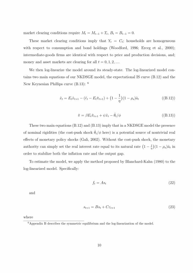
We then log-linearize the model around its steady-state. The log-linearized model con-

tains two main equations of our NKDSGE model, the expectational IS curve (B.12) and the

New Keynesian Phillips curve (B.13): 6

xt = Etxt+1 − (rt − Etπt+1) +(1− 1

η

)(1− ρa)at ((B.12))

π = βEtπt+1 + ψxt − θt/φ ((B.13))

These two main equations (B.12) and (B.13) imply that in a NKDSGE model the presence

of nominal rigidities (the cost-push shock θt/φ here) is a potential source of nontrivial real

effects of monetary policy shocks (Gali, 2002). Without the cost-push shock, the monetary

authority can simply set the real interest rate equal to its natural rate(1− 1

η

)(1− ρa)at in

order to stabilize both the inflation rate and the output gap.

To estimate the model, we apply the method proposed by Blanchard-Kahn (1980) to the

log-linearized model. Specifically:

ft = Ast (22)

and

st+1 = Bst + Cεt+1 (23)

where

6Appendix B describes the symmetric equilibrium and the log-linearization of the model.

10

ft = [gt, πt, rt]′

(24)

st = [yt−1, πt−1, rt−1, xt−1, gt−1, at, et, zt, εrt]′

(25)

εt+1 = [εat+1, εet+1, εzt+1, εrt+1]′

(26)

The empirical model consisting of (22) and (23) has three observable variables, output

growth, inflation, and the nominal short-term interest rate, and two unobservable variables

namely the de-trended output and the output gap. The model also consists of four different

shocks, the preference shock at, the cost-push shock7 et, the technology shock zt, and the

monetary policy shock εrt. All the shocks are assumed to be serially uncorrelated. In other

words, the covariance matrix of εt+1 is diagonal:

Eεt+1ε′t+1 =

σa 0 0 0

0 σe 0 0

0 0 σz 0

0 0 0 σr

(27)

The empirical model is in state-pace form and can be estimated via maximum likelihood

approach. The model is estimated based on quarterly data on real Gross Domestic Product

(GDP), GDP deflator, and 91-day Treasury Bills rate (TBILL) as the nominal short-term

interest rate over the period of 1970:1-2000:4. Before calculating the output (GDP) growth,

GDP is converted into per-capita form by dividing it with the size of population aged between

15-64. The data for seasonally adjusted real GDP, GDP deflator, and the 91-days TBILL

rate are obtained from the South African Reserve Bank Quarterly Bulletin.8 Note the base

year is the year of 2000. Series for population aged between 15-64 is obtained from World

Bank database.

7et = θt/φ is the transformed cost-push cost.8The plots of the three variables of concern, namely the per-capita growth rate, inflation and the Treasury

Bill rate, have been provided in the Appendix C.

11

4 Results

In this section, we compare the out-of-sample forecasting performance of the NKDSGE

model with the VARs, both Classical and Bayesian, in terms of the Root Mean Squared

Errors (RMSEs). At this stage, a few words need to be said regarding the choice of the

evaluation criterion for the out-of-sample forecasts generated from Bayesian models. As

Zellner (1986: 494) points out “the optimal Bayesian forecasts will differ depending upon

the loss function employed and the form of predictive probability density function”. In other

words, Bayesian forecasts are sensitive to the choice of the measure used to evaluate the out-

of-sample forecast errors. This fact was also observed in a recent study by Gupta (2006).

However, Zellner (1986) points out that the use of the mean of the predictive probability

density function for a series, is optimal relative to a squared error loss function and the

Mean Squared Error (MSE), and, hence, the RMSE is an appropriate measure to evaluate

performance of forecasts, when the mean of the predictive probability density function is

used.

But, before we proceed to the discussion of the forecasting performance of the alternative

models, it is important to lay out the basic structural differences and advantages of using

BVARs over traditional VARs for forecasting.

4.1 Classical and Bayesian VARs

An unrestricted VAR model, as suggested by Sims (1980), can be written as follows:

χt = C + λ(L)χt + εt (28)

where χ is a (n × 1) vector of variables being forecasted; λ(L) is a (n × n) polynominal

matrix in the backshift operator L with lag lenth p, i.e., λ(L) = λ1L+λ2L2 + ...+λpL

p; C is

a (n× 1) vector of constant terms; and ε is a (n× 1) vector of white-noise error terms. The

VAR model, thus, posits a set of relationships between the past lagged values of all variables

and the current value of each variable in the model.

One drawback of VAR models is that many parameters are needed to be estimated, some

12

of which may be insignificant. This problem of overparameterization, resulting in multi-

collinearity and a loss of degrees of freedom, leads to inefficient estimates and possibly large

out-of-sample forecasting errors. A popular approach to overcoming this overparameteriza-

tion, as described in Litterman (1981), Doan et al (1984), Todd (1984), Litterman (1986),

and Spencer (1993), is to use a Bayesian VAR (BVAR) model. Instead of eliminating longer

lags, the Bayesian method imposes restrictions on these coefficients by assuming that they

are more likely to be near zero than the coefficients on shorter lags. However, if there are

strong effects from less important variables, the data can override this assumption. The

restrictions are imposed by specifying normal prior distributions with zero means and small

standard deviations for all coefficients with the standard deviation decreasing as the lags

increase. The exception to this is, however, the coefficient on the first own lag of a variable,

which has a mean of unity. Litterman (1981) used a diffuse prior for the constant. This is

popularly referred to as the “Minnesota prior” due to its development at the University of

Minnesota and the Federal Reserve Bank at Minneapolis.

Formally, as discussed above, the Minnesota prior means take the following form:

βi ∼ N(1, σ2βi

)

βj ∼ N(0, σ2βj

)(29)

where βi represents the coefficients associated with the lagged dependent variables in each

equation of the VAR, while βj represents coefficients other than βi. The prior variances σ2βi

and σ2βj

, specify the uncertainty of the prior means, βi = 1 and βj = 0, respectively.

The specification of the standard deviation of the distribution of the prior imposed on

variable j in equation i at lag m, for all i, j and m, S(i, j, m), is given as follows:

S(i, j, m) = [w × g(m)× f(i, j)]σi

σj

(30)

where:

f(i, j) =

1 if i = j

kij otherwise, 0 ≤ kij ≤ 1

13

g(m) = m−d, d > 0

The term w is the measurement of standard deviation on the first own lag, and also indicates

the overall tightness. A decrease in the value of w results in a tighter prior. The function

g(m) measures the tightness on lag m relative to lag 1, and is assumed to have a harmonic

shape with a decay of d. An increas in d, tightens the prior as the number of lag increases. 9

The parameter f(i, j) represents the tightness of variable j in equation i relative to variable

i, thus, reducing the interaction parameter kij tightens the prior. σi and σj are the estimated

standard errors of the univariate autoregression for variable i and j respectively. In the case

of i 6= j, the standard deviations of the coefficients on lags are not scale invariant (Litterman,

1986b: 30). The ratio, σi

σjin (30), scales the variables so as to account for differences in the

units of magnitudes of the variables.10

4.2 Forecast Accuracy

Table 1 to 3 report the RMSEs from the NKDSGE model, along with those of the VARs.

When compared to the VAR and BVAR, the NKDSGE model does a better job in predicting

inflation than it does in predicting output growth and the nominal short-term interest rate

(TBILL). To be more precise, for inflation, the NKDSGE model outperforms both the un-

restricted VAR and the optimal BVAR 11, while for output growth and TBILL the RMSEs

generated from the NKDSGE model are larger than those generated from the unrestricted

VAR and the BVAR.

As far as the forecasting performances of the BVARs are concerned, except for inflation,

the optimal BVAR outperforms both the NKDSGE model and the unrestricted VAR. For

9In this paper, we set the overall tightness parameter (w) equal to 0.3, 0.2, and 0.1, and the harmonic lagdecay parameter (d) equal to 0.5, 1, and 2. These parameter values are chosen so that they are consistentwith the ones that used by Liu and Gupta (2007), and Liu et al. (2007).

10Note, the BVAR model is estimated using Theil’s (1971) mixed estimation technique, which involvessupplementing the data with prior information on the distribution of the coefficients. For each restrictionimposed on the parameter estimated, the number of observations and degrees of freedom are increased byone in an artificial way. Therefore, the loss of degrees of freedom associated with the unrestricted VAR isnot a concern in the BVAR.

11Here we only report the RMSEs from the optimal BVAR, i.e. a BVAR with a specific set of “hyperpa-rameters” for which we obtain the lowest RMSEs for each quarter.

14

inflation, the optimal BVAR only outperforms the unrestricted VAR. As shown in Table 1

to 3, for output growth and inflation a BVAR with a relatively tighter prior (w = 0.1, d = 1)

produces smaller forecast errors, whereas for TBILL the opposite holds. Interestingly, this

finding is different from Liu et al. (2007), in which a BVAR with a relatively loose prior

produces smaller forecast errors. Specifically, Liu et al. show that for all four variables

forecasted, namely output, consumption, investment and hours worked, a BVAR with the

most loose prior (w = 0.3, d = 0.5) outperforms the estimated Hansen(1985)–type DSGE

model and a Classical VAR.

Table 1. RMSE (2001Q1-2006Q4): Output Growth

QA 1 2 3 4 Average

NKDSGE 0.726 0.787 0.888 0.961 0.840

VAR (1) 0.756 0.700 0.797 0.851 0.776

BVAR (w=.1, d=1) 0.633 0.701 0.797 0.863 0.748

QA: Quarter Ahead; RMSE: Root Mean Squared Error (%).

Table 2. RMSE (2001Q1-2006Q4): Inflation

QA 1 2 3 4 Average

NKDSGE 0.280 0.349 0.422 0.439 0.373

VAR (1) 0.364 0.409 0.462 0.519 0.439

BVAR (w=.1, d=1) 0.312 0.402 0.467 0.520 0.425


Table 3. RMSE (2001Q1-2006Q4): TBILL

QA 1 2 3 4 Average

NKDSGE 0.914 1.586 2.067 2.406 1.743

VAR (1) 0.813 1.464 1.962 2.334 1.643

BVAR (w=.3, d=.5) 0.688 1.365 1.901 2.306 1.565


15

In order to evaluate the models’ forecast accuracy, we perform the across-model test

between the NKDSGE model and the VAR and BVAR models in pairs. The across-model

test is based on the statistic proposed by Diebold and Mariano (1995). The test statistic is

defined as the following. For instance, let {evt }T

t=1 denote the associated forecast errors from

the unrestricted VAR(1) model and {ekt }T

t=1 denote the forecast errors from the NKDSGE

model. The test statistic is then defined as s = lσl

, where l is the sample mean of the

“loss differentials” with {lt}Tt=1 obtained by using lt = (ev

t )2 − (ek

t )2 for all t = 1, 2, 3, ..., T ,

and where σl is the standard error of l. The s statistic is asymptotically distributed as a

standard normal random variable and can be estimated under the null hypothesis of equal

forecast accuracy, i.e. l = 0. Therefore, in this case, a positive value of s would suggest that

the NKDSGE model outperforms the unrestricted VAR(1) model in terms of out-of-sample

forecasting. Results are reported in Table 4. In general, the NKDSGE model does a better

job in predicting inflation than it does in predicting output growth and the nominal short-

term interest rate (TBILL). The differences between RMSEs generated from the NKDSGE

model and the VARs are minor, since most of the test statistics are insignificant.

16

Table 4. Across-Model Test Statistics

Quarters Ahead 1 2 3 4

(A) Output Growth

BVAR vs. NKDSGE -1.573 -1.271 -1.332 -1.257

BVAR vs. VAR(1) 0.913 -3.143∗ -0.002 -1.433

NKDSGE vs. VAR(1) -0.976 -1.710 -1.310 -1.270

(B) Inflation

BVAR vs. NKDSGE 0.760 0.541 0.358 1.078

BVAR vs. VAR(1) 1.145 0.533 -0.052 -0.747

NKDSGE vs. VAR(1) 0.889 0.588 0.355 1.019

(C) TBILL

BVAR vs. NKDSGE -2.226∗ -1.542 -0.896 -0.547

BVAR vs. VAR(1) 1.377 1.009 0.769 0.576

NKDSGE vs. VAR(1) -2.463∗ -1.010 -0.577 -0.371

Note:∗ indicates significance at the 5 percent level.

5 Conclusion

In this paper, we show that, besides its usual usage for policy analysis, a small-scale NKDSGE

model has a future for forecasting. We show that the NKDSGE model outperforms both

the Classical and Bayesian variants of the VARs in forecasting inflation, but not for output

growth and the nominal short-term interest rate. However, the differences of the forecast

errors are minor. The indicated success of the NKDSGE model for predicting inflation is

important, especially in the context of South Africa — an economy targeting inflation.

As suggested by Smets and Wouters (2004), a NKDSGE model estimated by Bayesian

techniques can become an useful tool in the forecasting kit for central banks. In this back-

drop, further research will concentrate on developing an estimated NKDSGE model based

on Bayesian techniques. In addition, future research in this area will also aim to extend the

17

current framework into that of a small open economy.

18

References

Barro, R. J. and D. B. Gordon, 1983. Rules, Discretion, and Reputation in a Model of

Monetary Policy. Journal of Monetary Economics, 12: 101-121.

Blanchard, O. J. and C. M. Kahn, 1980. The solution of linear difference models under

rational expectations. Econometrica, 48: 1305-1311.

Christiano, L. J., Eichenbaum, M. and C. L. Evans, 2005. Nominal rigidities and the dynamic

effects of a shock to monetary policy. Journal of Political Economy, 113(11): 1-45.

Clarida, R., Gali, J. and M. Gertler, 1999. The science of monetary policy: A new Keyesian

perspective. Journal of Economic literature, 37: 1661-1707.

Cogley, T. and J. M. Nason, 1995. Output dynamics in real-business-cycle models. American

Economic Review, 85(3): 492-511.

Diebold, F. X. and R. S. Mariano, 1995. Comparing predictive accuracy. Journal of Business

and Economic Statistics, 13: 253-263.

Dixit, A. and J. Stiglitz, 1977. Monopolistic competition and optimum product diversity.

American Economic Review, 67(3): 297-308.

Doan, T., Litterman, R. B. and C. Smis, 1984. Forecasting and conditional projection using

realistic prior distributions. Econometric Reviews, 3: 1-144.

Dotsey, M. and R. G. King, 2001. Pricing production and persistence. National Bureau of

Economic Research, Working Paper, No. 8407. Cambridge.

Erceg, C. J., Henderson, D. W. and A. T. Levin, 2000. Optimal monetary policy with

staggered wage and price contracts. Journal of Monetary Economy, 46(2): 281-313.

Gali, J., 2002. New perspectives on monetary policy, inflation, and the business cycle.

National Bureau of Economic Research, Working Paper, No. 8767. Cambridge.

19

Goodfriend, M. and R. G. King, 1997. The new neoclassical synthesis and the role of

monetary policy. National Bureau of Economic Research, Macroeconomics Annual, 231-283.

Cambridge.

Gupta, R., 2006. Forecasting the South African economy with VARs and VECMs. South

African Journal of Economics, 74(4): 611-628.

Hansen, G. D., 1985. Indivisible labor and the business cycle. Journal of Monetary Eco-

nomics, 16: 309-327.

Hodrick, R. J. and E. C. Precott, 1997. Postwar U.S. business cycle: an empirical investiga-

tion. Journal of Money, Credit, and Banking, 29: 1-16.

Kydland, F. E. and E. C. Prescott, 1982. Time to build and aggregate fluctuations. Econo-

metrica, 50(6): 1345-1370.

McCallum, T. M. and E. Nelson, 1999. An optimizing IS-LM specification for monetary

policy and business cycle analysis. Journal of Money, Credit and Banking, 31(3): 296-316.

Nelson, C. R. and C. Plosser, 1982. Trend and random walks in macro-economic time series.

Bank of Canada, Technical Report, No. 50. Ottawa.

Ireland, P. N., 2001. Money’s role in the monetary business cycle. National Bureau of

Economic Research, Working Paper, No. 8115. Cambridge.

—, 2004. Technology shocks in the new Keynesian model. National Bureau of Economic

Research, Working Paper, No. 10309. Cambridge.

Laxton, D. and R. Tetlow, 1992. A simple multivariate filter for the measurement of potential

output. Bank of Canada, Working Paper, No. 93-7. Ottawa.

Litterman, R. B., 1981. A Bayesian procedure for forecasting with vector autoregressions.

Working Paper, Federal Reserve Bank of Minneapolis.

20

—, 1986a. A statistical approach to economic forecasting. Journal of Business and Statistics,

4(1): 1-4.

—, 1986b. Forecasting with Bayesian vector autoregressions—five years of experiece. Journal

of Business and Statistics, 4(1): 25-38.

Liu G. L. and R. Gupta, 2007. A small-skill DSGE model for forecasting the South Africa

economy. South Africa Journal of Journal of Economics, 75(2): 179-193.

Liu G. L., Gupta, R. and E. Schaling, 2007. Forecasting the South African economy: A

DSGE-VAR approach. Economic Research Southern Africa, Working Paper, No. 51. Cape

Town.

Rogoff, K., 1985. The Optimal Degree of Commitment to an Intermediate Monetary Target.

Quarterly Journal of Economics, 100: 1169-89.

Rotemberg, J. J., 1982. Sticky prices in the United States. Journal of Political Economy,

90: 1187-1211.

Rotemberg, J. J. and M. Woodford, 1997. An optimization-based econometric framework for

the evaluation of monetary policy. National Bureau of Economic Research, Macroeconomics

Annual, 297-346. Cambridge.

Sims, C. A., 1980. Macroeconomics and reality. Econometrica, 48(January): 1-48.

Smets, F., 1998. Output gap uncertainty: does it matter for the Taylor rule? Bank for

International Settlements, Working Paper, No. 60. Basle.

Smets, F. and R. Wouters, 2003. An estimated dynamic stochastic general equilibrium model

of the euro area. Journal of the European Economic Association, 1(5): 1123-1175.

—, 2004. Forecasting with a Bayesian DSGE model: an application to the Euro area.

European Central Banks, Working Paper, No. 389.

21

Taylor, J. B., 1993. Discretion versus policy rules in practice. Carnegie-Rochester Conference

Series on Public Policy, 39: 195-214.

Theil, H., 1971. Principles of econometrics. New York: John Wiley.

Woodford, M., 1996. Control of the public debt: A requirement for price stability? National

Bureau of Economic Research, Working Paper, No. 5684. Cambridge.

Zellner, A., 1986. A tale of forecasting 1001 series: The Bayesian knight strikes again.

International Journal of Forecasting, 2(4): 494-494.

22

A Optimization

A.1 Household

In the NKDSGE model, the representative household chooses {Ct, ht,Mt

Pt, Bt

Pt} to maximize

the utility function (1):

E

∞∑t=0

βt[atlog(Ct) + log

(Mt

Pt

)− (1

η

)hη

t

], 0 < β < 1, η ≥ 1, ((1))

subject to the budget constraint (3):

Ct +Bt

rtPt

=Wt

Pt

ht +Bt−1

Pt

+ Dt + Tt − Mt −Mt−1

Pt

((3))

The resulting Bellman’s equation is as follows:

V (Mt−1, Bt−1, at, Zt, εrt) = max[atlog(Ct)+log(Mt

Pt

)−(1

η

)hη

t +βEtV (Mt, Bt, at+1, Zt+1, εrt+1)]

(A.1)

Substituting Ct from (3) into (A.1) and solving this problem yields the following first

order condition (FOC) for hours worked:

∂V (Mt−1, Bt−1, at, Zt, εrt)

∂ht

= 0 (A.2)

at

Ct

Wt

Pt

− hη−1t = 0 (A.3)

Wt

Pt

= a−1t Cth

η−1t (A.4)

The FOC for bond holdings is given as follows:

23


∂Bt

= 0 (A.5)

at

Ct

(− 1

rtPt

) +∂βEtV (Mt, Bt, at+1, Zt+1, εrt+1)

∂Bt

= 0 (A.6)

The associated envelope condition is:


∂Bt−1

=at

Ct

1

Pt

(A.7)

Updating (A.7) and combining with (A.6) yields

at

Ct

= rtβEt

[at+1

( 1

Ct+1

)( Pt

Pt+1

)](A.8)

FOC for money holdings can be derived as follows:


∂Mt

= 0 (A.9)

at

Ct

(−1)1

Pt

+1

Mt

+∂βEtV (Mt, Bt, at+1, Zt+1, εrt+1)

∂Mt

= 0 (A.10)

The associated envelope condition is:


∂Mt−1

=at

Ct

1

Pt

(A.11)

Updating (A.11) and combining with (A.10), we have:

at

Ct

=Pt

Mt

+ βEt(at+1

Ct+1

Pt

Pt+1

) (A.12)

Pt

Mt

= βEt(Pt

Pt+1

)− at

Ct

(A.13)

Using (A.8):

24

Mt

Pt

= a−1t Ct[rt/(rt − 1)] (A.14)

A.2 Final goods firm

A representative firm produces the final good Yt using intermediate goods Yjt according to

the CES production function:

Yt =

(∫ 1

0

Yθt−1

θtjt dj

) θtθt−1

(A.15)

The firm maximizes its profit:

maxYjt

{Yt − 1

Pt

∫ 1

0

PjtYjt

}(A.16)

Alternatively, the firm minimizes its expenditure given the production constraint. The

Lagrangean for the firm is given by the following expression:

L =

∫ 1

0

PjtYjtdj − Pt

[Yt −

(∫ 1

0

Yθt−1

θtjt dj

) θtθt−1 ]

(A.17)

Setting ∂L∂Yjt

= 0, yields:

Pjt = Pt∂Yt

∂Yjt

(A.18)

where:

∂Yt

∂Yjt

=θt

θt − 1

(∫ 1

0

Yθt−1

θtjt dj

) 1θt−1 (θt − 1

θt

)Y−1/θt

jt (A.19)

=( Yt

Yjt

)1/θt

(A.20)

Substituting (A.20) into (A.18), yields:

Yjt =(Pjt

Pt

)−θt

Yt (A.21)

25

Here, given Euler’s theorem, profits in this sector must equal to zero in equilibrium:

PtYt =

∫ 1

0

PjtYjtdj (A.22)

Solving for the optimal price of the final-goods Yt, yields:

Pt =(∫ 1

0

P 1−θtjt dj

) 11−θt (A.23)

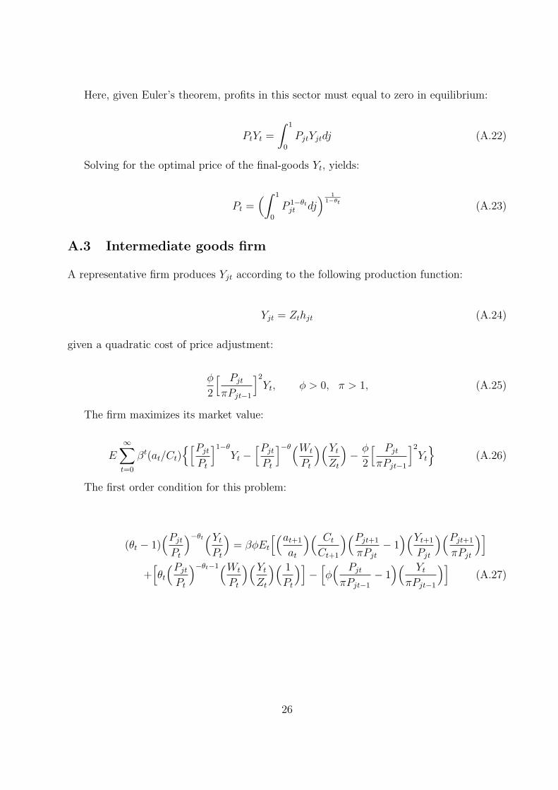
A.3 Intermediate goods firm

A representative firm produces Yjt according to the following production function:

Yjt = Zthjt (A.24)

given a quadratic cost of price adjustment:

φ

2

[ Pjt

πPjt−1

]2

Yt, φ > 0, π > 1, (A.25)

The firm maximizes its market value:

E

∞∑t=0

βt(at/Ct){[Pjt

Pt

]1−θ

Yt −[Pjt

Pt

]−θ(Wt

Pt

)(Yt

Zt

)− φ

2

[ Pjt

πPjt−1

]2

Yt

}(A.26)

The first order condition for this problem:

(θt − 1)(Pjt

Pt

)−θt(Yt

Pt

)= βφEt

[(at+1

at

)( Ct

Ct+1

)(Pjt+1

πPjt

− 1)(Yt+1

Pjt

)(Pjt+1

πPjt

)]

+[θt

(Pjt

Pt

)−θt−1(Wt

Pt

)(Yt

Zt

)( 1

Pt

)]−

[φ( Pjt

πPjt−1

− 1)( Yt

πPjt−1

)](A.27)

26

B The Log-linear Equilibrium

B.1 Symmetric Equilibrium

In a symmetric equilibrium, the model can be summarized as follows:

Yt = Ztht (B.1)

Wt

Pt

= a−1t Cth

η−1t (B.2)

at

Ct

= rtβEt

[at+1

( 1

Ct+1

)( Pt

Pt+1

)](B.3)

Mt

Pt

= a−1t Ct[rt/(rt − 1)] (B.4)

log(at) = ρalog(at−1) + εat (B.5)

logθt = (1− ρθ)logθ + ρθlogθt−1 + εθt (B.6)

logZt = logZ + logZt−1 + εzt (B.7)

0 = (1− θt)(Pjt

Pt

)−θt(Yt

Pt

)+ βφEt

[(at+1

at

)( Ct

Ct+1

)(Pjt+1

πPjt

− 1)(Yt+1

Pjt

)(Pjt+1

πPjt

)]

+[θt

(Pjt

Pt

)−θt−1(Wt

Pt

)(Yt

Zt

)( 1

Pt

)]−

[φ( Pjt

πPjt−1

− 1)( Yt

πPjt−1

)](B.8)

B.2 Log-linearization

In our complete model, equations (B.1)-(B.8) together with the output gap equation (21)

describe the behavior of the endogenous variables Yt, Ct, πt, rt, and xt, and the three exoge-

nous shocks at, θt, and Zt. Yt, Ct, and Zt are stochastically detrended so that yt = Yt/Zt,

ct = Ct/Zt, and zt = Zt/Zt−1 are stationary.

In the absence of shocks, the economy converges to a steady-state growth path, in which

yt = y, ct = c, πt = π, rt = r, xt = x, gt = g, at = a, θt = θ, and zt = z for all t = 0, 1, 2, ....

Therefore, in steady-state we have:

27

y =[a(θ − 1

θ

)] 1η

(B.9)

r =( z

β

)π (B.10)

x =(θ − 1

θ

) 1η

(B.11)

Using first-order Taylor approximation to rewrite all the equations of the model, we have:

xt = Etxt+1 − (rt − Etπt+1) +(1− 1

η

)(1− ρa)at (B.12)

π = βEtπt+1 + ψxt − θt/φ, ψ = η(θ − 1

φ

)(B.13)

xt = yt − 1

ηat (B.14)

gt = yt − yt−1 + zt (B.15)

at = ρaat−1 + εat (B.16)

θt = ρθθt−1 + εθt (B.17)

zt = εzt (B.18)

28

A New-Keynesian DSGE Model for Forecasting the South ...

Documents

Transcript of A New-Keynesian DSGE Model for Forecasting the South ...