Exchange rate forecasting with DSGE models · Exchange rate forecasting with DSGE models Michele...
47
NBP Working Paper No. 260 Exchange rate forecasting with DSGE models Michele Ca’ Zorzi, Marcin Kolasa, Michał Rubaszek
Transcript of Exchange rate forecasting with DSGE models · Exchange rate forecasting with DSGE models Michele...
NBP Working Paper No. 260
Exchange rate forecasting with DSGE models
Michele Ca’ Zorzi, Marcin Kolasa, Michał Rubaszek
Economic Research DepartmentWarsaw, 2017
NBP Working Paper No. 260
Exchange rate forecasting with DSGE models
Michele Ca’ Zorzi, Marcin Kolasa, Michał Rubaszek

Published by: Narodowy Bank Polski Education & Publishing Department ul. Świętokrzyska 11/21 00-919 Warszawa, Poland phone +48 22 185 23 35 www.nbp.pl
ISSN 2084-624X
© Copyright Narodowy Bank Polski, 2017
Michele Ca’ Zorzi – European Central Bank [email protected]
Marcin Kolasa – Narodowy Bank Polski and Warsaw School of Economics [email protected]
Michał Rubaszek – Narodowy Bank Polski and Warsaw School of Economics [email protected]
We would like to thank Charles Engel, Gianni Amisano, Luca Dedola, Alistair Dieppe, Mike Moss, Carl Sholl, Livio Stracca, Grzegorz Szafranski, Cedric Tille and two anonymous referees for excellent comments and suggestions. We are also grateful to the authors of The Bear toolbox (Dieppe et al., 2016) for granting us access to selected source codes. The paper was presented at Narodowy Bank Polski (Warsaw, September 2015), the European Central Bank (Frankfurt, October 2015), the 16th IWH-CIREQ Macroeconometric Workshop (Halle, December 2015), Norges Bank (Oslo, January 2016), the 4th International Symposium in Computational Economics and Finance (Paris, April 2016), the 36th International Symposium on Forecasting (Santander, June 2016) and the 31th annual congress of the European Economic Association (Geneva, August 2016). We thank the participants for useful discussions. The views expressed in this paper are those of the authors and do not necessarily reflect opinions of the institutions to which they are affiliated.
3NBP Working Paper No. 260
ContentsAbstract 4
Non-technical summary 5
1 Introduction 7
2 Round-up of forecasting methodologies 10
3 Data 13
4 Results for the real exchange rate 14
5 Results for the nominal exchange rate 19
6 Conclusions 23
References 24
List of Tables
1 Variable description and data sources 27
2 Root mean squared forecast error (RMSFE) for the RER 28
3 Forecast efficiency test for the RER 29
4 Comparison of one and 24-quarter ahead forecasts and realizations for the RER 30
5 Pace of mean reversion for the RER 31
6 RMSFE for the NER 32
7 RMSFE relative to the RW in a Monte Carlo experiment 32
8 RMSFE for the RPI 33
9 Selected moments from the DSGE model 34
10 RMSFE for the nominal exchange rate from partially consistent models 35
List of Figures
1 Realizations and forecasts at a one-quarter horizon for the real exchange rate 36
2 Realizations and forecasts at a six-year horizon for the real exchange rate 37
3 Sequential real exchange rate forecasts 38
4 Recursive mean (AR-fixed) and sequential steady state estimates (MBVAR and DSGE) for the real exchange rate 39
5 Speed of reversion to equilibrium for different shocks in the DSGE model 40
6 Sequential forecasts from the DSGE model 41
7 Response of RER, NER and RPI to structural shocks in the DSGE model for the US economy 42
Appendix
A Log-linearized equations of the DSGE model 43
B Measurement equations used to estimate the DSGE model 44
C Calibration and estimation details 44

Narodowy Bank Polski4
Abstract
We run an exchange rate forecasting “horse race”, which highlights that three principles hold.First, forecasts should not replicate the high volatility of exchange rates observed in sample.Second, models should exploit the mean reversion of the real exchange rate over long horizons.Third, they should account for the international price co-movement seen in the data. Abiding bythe first two principles an open-economy dynamic stochastic general equilibrium (DSGE) modelperforms well in forecasting the real but not the nominal exchange rate. Only approaches thatconform to all three principles tend to outperform the random walk.
Keywords: Forecasting; exchange rates; New Open Economy Macroeconomics; mean reversion.
JEL classification: C32; F31; F41; F47.
4
Non-technical summary
Economic theory provides policymakers with clear guidance on how the competitiveness chan-
nel operates in the aftermath of a wide set of disturbances, such as monetary, productivity, risk
premium or foreign shocks. However, there is a cloud hanging over this aspect of international
economics, namely that these conjectures may have limited empirical significance, given the sys-
tematic failure of macro models to beat even the naıve random walk in exchange rate forecasting.
The question then naturally arises of whether international macro models are rich enough to be
meaningful. Layers of complexity are typically added to improve their realism. For example,
including in the features of the model the currency of trade invoicing may help the model to
capture better the degree of exchange rate pass-through. Similarly, distinguishing the currency
of denomination of asset and liabilities, may lead to a better description of the dynamics of
external debt, which may be essential to better understand real exchange rate movements in
emerging countries. On the other hand, imposing too many restrictions on the data generating
process, either theoretically or in the estimation phase, may prove disadvantageous from a pure
forecasting perspective given the higher number of estimated parameters.
Every cloud has a silver lining, however. The exchange rate disconnect puzzle has spurred
economists to look for new directions of research with success. Open-economy dynamic stochastic
general equilibrium (DSGE) models are clearly a major accomplishment from the theoretical
perspective. The empirical literature has also shown why, by properly accounting for estimation
error, exchange rate models may be better than we usually think. The consensus in the literature
has also shifted back to the pre-1970s view that real exchange rates do not move randomly, but
tend to revert to a slow-moving equilibrium. This particular finding raises a question, however.
Why don’t the mean-reverting properties of the real exchange rate, which are embedded in most
new open-economy models, give them an edge in exchange rate forecasting vis-a-vis the random
walk?
The aim of this paper is to answer this very question. We evaluate the forecasting perfor-
mance of a state-of-the-art open-economy DSGE model. Our goal is to cross-check whether this
framework, albeit conceptually more appealing than the macro models of the 1970s, has the
same disappointing performance out of sample. The results are encouraging.
First the good news: we find that our preferred DSGE model forecasts real exchange rates
consistently better than the RW for three out of five countries at medium-term horizons and
performs comparably for the other two. This suggests that a mean reverting real exchange
rate, which is an inherent property of our preferred DSGE model, is a helpful feature rather
than an obstacle from a forecasting perspective. Moreover, we indicate that there are two other
forecasting tools that are more difficult to beat than the RW. We label the first one AR-fixed
since it is a simple autoregressive process of order one, where the autoregressive parameter is
fixed by the modeler. The other successful competitor at medium-term horizons is a Bayesian
VAR model, in which the modeler sets the prior that the real exchange rate reverts to its sample
mean (MBVAR model).
Two reasons explain their success. Firstly, the AR-fixed model, and to a lesser extent the
5
5NBP Working Paper No. 260
Abstract
We run an exchange rate forecasting “horse race”, which highlights that three principles hold.First, forecasts should not replicate the high volatility of exchange rates observed in sample.Second, models should exploit the mean reversion of the real exchange rate over long horizons.Third, they should account for the international price co-movement seen in the data. Abiding bythe first two principles an open-economy dynamic stochastic general equilibrium (DSGE) modelperforms well in forecasting the real but not the nominal exchange rate. Only approaches thatconform to all three principles tend to outperform the random walk.
Keywords: Forecasting; exchange rates; New Open Economy Macroeconomics; mean reversion.
JEL classification: C32; F31; F41; F47.
4
Non-technical summary
Economic theory provides policymakers with clear guidance on how the competitiveness chan-
nel operates in the aftermath of a wide set of disturbances, such as monetary, productivity, risk
premium or foreign shocks. However, there is a cloud hanging over this aspect of international
economics, namely that these conjectures may have limited empirical significance, given the sys-
tematic failure of macro models to beat even the naıve random walk in exchange rate forecasting.
The question then naturally arises of whether international macro models are rich enough to be
meaningful. Layers of complexity are typically added to improve their realism. For example,
including in the features of the model the currency of trade invoicing may help the model to
capture better the degree of exchange rate pass-through. Similarly, distinguishing the currency
of denomination of asset and liabilities, may lead to a better description of the dynamics of
external debt, which may be essential to better understand real exchange rate movements in
emerging countries. On the other hand, imposing too many restrictions on the data generating
process, either theoretically or in the estimation phase, may prove disadvantageous from a pure
forecasting perspective given the higher number of estimated parameters.
Every cloud has a silver lining, however. The exchange rate disconnect puzzle has spurred
economists to look for new directions of research with success. Open-economy dynamic stochastic
general equilibrium (DSGE) models are clearly a major accomplishment from the theoretical
perspective. The empirical literature has also shown why, by properly accounting for estimation
error, exchange rate models may be better than we usually think. The consensus in the literature
has also shifted back to the pre-1970s view that real exchange rates do not move randomly, but
tend to revert to a slow-moving equilibrium. This particular finding raises a question, however.
Why don’t the mean-reverting properties of the real exchange rate, which are embedded in most
new open-economy models, give them an edge in exchange rate forecasting vis-a-vis the random
walk?
The aim of this paper is to answer this very question. We evaluate the forecasting perfor-
mance of a state-of-the-art open-economy DSGE model. Our goal is to cross-check whether this
framework, albeit conceptually more appealing than the macro models of the 1970s, has the
same disappointing performance out of sample. The results are encouraging.
First the good news: we find that our preferred DSGE model forecasts real exchange rates
consistently better than the RW for three out of five countries at medium-term horizons and
performs comparably for the other two. This suggests that a mean reverting real exchange
rate, which is an inherent property of our preferred DSGE model, is a helpful feature rather
than an obstacle from a forecasting perspective. Moreover, we indicate that there are two other
forecasting tools that are more difficult to beat than the RW. We label the first one AR-fixed
since it is a simple autoregressive process of order one, where the autoregressive parameter is
fixed by the modeler. The other successful competitor at medium-term horizons is a Bayesian
VAR model, in which the modeler sets the prior that the real exchange rate reverts to its sample
mean (MBVAR model).
Two reasons explain their success. Firstly, the AR-fixed model, and to a lesser extent the
5
Narodowy Bank Polski6
Non-technical summary
MBVAR model, minimizes the errors at short horizons by mimicking the RW. Secondly, both
models exploit the mean reversion of real exchange rates at longer horizons (in line with long-term
Purchasing Power Parity). The way they do this is model specific. The AR-fixed model foresees a
constant adjustment of the real exchange rate to the recursive sample mean (“trivial dynamics”).
The MBVAR model projects instead a richer adjustment process towards the recursive steady
state (“no economic story”). By contrast, the DSGE model foresees a dynamic of adjustment
to the steady state which depends on the type of structural shocks that have tilted the real
exchange rate away from its equilibrium (“macroeconomic story”).
The key appeal of the DSGE model is that it provides a consistent macroeconomic expla-
nation of how a wide set of variables adjust towards their equilibrium. The real exchange rate
adjustment implied by the model is consistent with current account sustainability and conver-
gence of inflation to its steady state. The concept of equilibrium exchange rate is also well
defined. Empirically the model captures better the directional change of the real exchange rate.
There is however a price in terms of complexity, which on the whole leads to just a minimal
improvement in its forecasting performance relative to its closest competitors.
The bad news is that, if used consistently, the DSGE model encounters severe difficulties in
forecasting nominal exchange rates. The reason is that it wrongly projects the relative adjust-
ment of domestic and foreign prices. This negative result is nonetheless insightful because it
helps us to reconcile the forecastability of real exchange rates with the exchange rate disconnect
puzzle. The difficulty of macro models to beat the random walk in exchange rate forecasting
lies to a large extent in their difficulty in forecasting well domestic and foreign prices and their
co-movement. Therefore, it is not surprising that the random walk can be beaten also in nominal
exchange rate forecasting, but not with a fully consistent DSGE model. This can be accom-
plished by employing the real exchange rate forecasts delivered by our three best models and, as
a second step, assuming that all of the adjustment takes place via the nominal exchange rate.
This reveals that the random walk is not invincible even at horizons of one or two years.
6
1 Introduction
There is hardly anything more fascinating or nerve-wracking in international finance than at-
tempting to understand exchange rates. Little can be said about the international transmission
of shocks or the cross-border impact of monetary policy without a good understanding of what
drives them. But how much do we really know? We tend to lean on economic theory to tell
us a plausible story of how exchange rates react to a set of model-based disturbances, such as
monetary, productivity, risk premium and foreign shocks. Yet since the seminal paper by Meese
and Rogoff (1983) there is a dark cloud hanging over open-economy macro models because of
their failure to beat even the naıve random walk (RW) in forecasting the nominal exchange rate
(NER). Over the years, several studies have evaluated the robustness of this result using a large
variety of methodologies (for surveys, see Cheung et al., 2005; Rossi, 2013). One of the most
positive findings of the literature is that the ability of exchange rate models to beat the RW tends
to strengthen for larger datasets (Mark, 1995; Engel, 2014; Ince, 2014). Our interpretation of
this result is that the dismal forecasting performance of exchange rate models can be attributed
to some extent to estimation error.
Not all exchange rate theories have been discredited equally. Purchasing power parity (PPP)
theory was reappraised as a long-term concept (Taylor and Taylor, 2004). Notwithstanding the
unreliability of unit root tests, owing to their size distortion and low power (Engel, 2000), the
majority of the literature now takes for granted that the real exchange rate (RER) has an im-
portant mean reverting component and focuses instead on how to explain its slow adjustment
process. Recent papers have argued that the mean reverting property of the RER can be ex-
ploited to beat the RW both in RER and NER forecasting (Engel et al., 2008; Ca’ Zorzi et al.,
2016; Cheung et al., 2017). This highlights how simple measures of exchange rate disequilib-
ria not only signal potential economic imbalances but also tell us something about the future
direction of NER movements.
Albeit very promising, these developments are a far cry from what economists desire, namely
a fully-fledged macro model that has some predictive power. Economic theory has evolved pro-
foundly over the past 30 years. A clear highlight has been the development of richly specified
open-economy dynamic stochastic general equilibrium (DSGE) models. Since the seminal work
of Obstfeld and Rogoff (1995), a large variety of different specifications have been proposed
through the development of two-country (Devereux and Engel, 2003) or small open-economy
models (Gali and Monacelli, 2005). Thanks to the progress achieved by the econometric litera-
ture, complex DSGE models can now be brought to the data via the use of advanced estimation
techniques (An and Schorfheide, 2007). These advances, however, beg the question: is this rich
theoretical structure a help or a hindrance to forecasting real and nominal exchange rates?
The answer it not available since these models are seldom included in exchange rate forecast-
ing races. The two exceptions that we are aware of are the studies by Adolfson et al. (2007b)
and Christoffel et al. (2011), which evaluate forecasts from DSGE models for the euro area.
They show that, at least in the case of the euro, the RER can be forecasted more accurately
with an open-economy DSGE model than with the RW or with Bayesian vector autoregressions
7
7NBP Working Paper No. 260
Chapter 1
MBVAR model, minimizes the errors at short horizons by mimicking the RW. Secondly, both
models exploit the mean reversion of real exchange rates at longer horizons (in line with long-term
Purchasing Power Parity). The way they do this is model specific. The AR-fixed model foresees a
constant adjustment of the real exchange rate to the recursive sample mean (“trivial dynamics”).
The MBVAR model projects instead a richer adjustment process towards the recursive steady
state (“no economic story”). By contrast, the DSGE model foresees a dynamic of adjustment
to the steady state which depends on the type of structural shocks that have tilted the real
exchange rate away from its equilibrium (“macroeconomic story”).
The key appeal of the DSGE model is that it provides a consistent macroeconomic expla-
nation of how a wide set of variables adjust towards their equilibrium. The real exchange rate
adjustment implied by the model is consistent with current account sustainability and conver-
gence of inflation to its steady state. The concept of equilibrium exchange rate is also well
defined. Empirically the model captures better the directional change of the real exchange rate.
There is however a price in terms of complexity, which on the whole leads to just a minimal
improvement in its forecasting performance relative to its closest competitors.
The bad news is that, if used consistently, the DSGE model encounters severe difficulties in
forecasting nominal exchange rates. The reason is that it wrongly projects the relative adjust-
ment of domestic and foreign prices. This negative result is nonetheless insightful because it
helps us to reconcile the forecastability of real exchange rates with the exchange rate disconnect
puzzle. The difficulty of macro models to beat the random walk in exchange rate forecasting
lies to a large extent in their difficulty in forecasting well domestic and foreign prices and their
co-movement. Therefore, it is not surprising that the random walk can be beaten also in nominal
exchange rate forecasting, but not with a fully consistent DSGE model. This can be accom-
plished by employing the real exchange rate forecasts delivered by our three best models and, as
a second step, assuming that all of the adjustment takes place via the nominal exchange rate.
This reveals that the random walk is not invincible even at horizons of one or two years.
6
1 Introduction
There is hardly anything more fascinating or nerve-wracking in international finance than at-
tempting to understand exchange rates. Little can be said about the international transmission
of shocks or the cross-border impact of monetary policy without a good understanding of what
drives them. But how much do we really know? We tend to lean on economic theory to tell
us a plausible story of how exchange rates react to a set of model-based disturbances, such as
monetary, productivity, risk premium and foreign shocks. Yet since the seminal paper by Meese
and Rogoff (1983) there is a dark cloud hanging over open-economy macro models because of
their failure to beat even the naıve random walk (RW) in forecasting the nominal exchange rate
(NER). Over the years, several studies have evaluated the robustness of this result using a large
variety of methodologies (for surveys, see Cheung et al., 2005; Rossi, 2013). One of the most
positive findings of the literature is that the ability of exchange rate models to beat the RW tends
to strengthen for larger datasets (Mark, 1995; Engel, 2014; Ince, 2014). Our interpretation of
this result is that the dismal forecasting performance of exchange rate models can be attributed
to some extent to estimation error.
Not all exchange rate theories have been discredited equally. Purchasing power parity (PPP)
theory was reappraised as a long-term concept (Taylor and Taylor, 2004). Notwithstanding the
unreliability of unit root tests, owing to their size distortion and low power (Engel, 2000), the
majority of the literature now takes for granted that the real exchange rate (RER) has an im-
portant mean reverting component and focuses instead on how to explain its slow adjustment
process. Recent papers have argued that the mean reverting property of the RER can be ex-
ploited to beat the RW both in RER and NER forecasting (Engel et al., 2008; Ca’ Zorzi et al.,
2016; Cheung et al., 2017). This highlights how simple measures of exchange rate disequilib-
ria not only signal potential economic imbalances but also tell us something about the future
direction of NER movements.
Albeit very promising, these developments are a far cry from what economists desire, namely
a fully-fledged macro model that has some predictive power. Economic theory has evolved pro-
foundly over the past 30 years. A clear highlight has been the development of richly specified
open-economy dynamic stochastic general equilibrium (DSGE) models. Since the seminal work
of Obstfeld and Rogoff (1995), a large variety of different specifications have been proposed
through the development of two-country (Devereux and Engel, 2003) or small open-economy
models (Gali and Monacelli, 2005). Thanks to the progress achieved by the econometric litera-
ture, complex DSGE models can now be brought to the data via the use of advanced estimation
techniques (An and Schorfheide, 2007). These advances, however, beg the question: is this rich
theoretical structure a help or a hindrance to forecasting real and nominal exchange rates?
The answer it not available since these models are seldom included in exchange rate forecast-
ing races. The two exceptions that we are aware of are the studies by Adolfson et al. (2007b)
and Christoffel et al. (2011), which evaluate forecasts from DSGE models for the euro area.
They show that, at least in the case of the euro, the RER can be forecasted more accurately
with an open-economy DSGE model than with the RW or with Bayesian vector autoregressions
7
Narodowy Bank Polski8
(BVAR). To the extent that this result stays robust for other currencies, a longer sample span
and tougher benchmarks, and can be extended to forecasting the NER, it would be clearly an
important step forward.
The contribution of this paper is to provide a thorough evaluation of whether state-of-
the-art open economy DSGE models can be successful in forecasting both real and nominal
exchange rates. From the possible options at our disposal, we chose the open-economy framework
developed by Justiniano and Preston (2010b), because it appears particularly well designed and
suited to our aims. A central question is whether models such as this have any chances of
forecasting exchange rates accurately. Ex ante there is reason to doubt it, given the serious
difficulties that they have in accounting for international co-movement of key macroeconomic
variables (Justiniano and Preston, 2010a) and in forecasting domestic variables (Kolasa and
Rubaszek, 2016). There are, however, two reasons for cautious optimism. First, long-term PPP
is an intrinsic feature of open-economy DSGE models, which should give them an edge over the
RW in an exchange rate forecasting race. Second, they describe well the key role of the NER in
driving the RER towards its equilibrium (Engel, 2012; Eichenbaum et al., 2017).
To have a comprehensive set of results, we estimate the open-economy DSGE model sepa-
rately for Australia, Canada, the United Kingdom, the euro area and the United States. The
country coverage, the long evaluation sample and a set of diagnostic tools make our study ar-
guably more comprehensive than any previous evaluations of the forecasting performance of
DSGE models, especially in an open-economy context. We also apply one of the key lessons of
the recent forecasting literature and avoid easy sparring partners (Giacomini, 2015) by bringing
six competing models into the exchange rate forecasting race. The first is the “twin” DSGE
model, which is identical from a theoretical perspective, but allows for a linear trend in the RER
to improve the in-sample fit. We include this specification in our forecasting contest as it is a
common practice to detrend the RER (and other variables) before estimation, as can be seen,
for example, in Bergin (2003, 2006) and Justiniano and Preston (2010b). Next, we have three
BVAR models. Two are standard, while the third exploits the methodology of Villani (2009)
to elicit the prior that the RER reverts to its recursive mean (mean-adjusted Bayesian vector
autoregression, MBVAR). The last two models in the forecasting race are atheoretical. One is
the classical RW model, which remains the most popular benchmark in exchange rate forecast-
ing competitions. The other is a simple first-order autoregressive process, which assumes that
the forecasted variable gradually converges to its mean at the speed that is set by the modeler.
We label this model AR-fixed, in line with Faust and Wright (2013) in their work on inflation
forecasting.
The key insight of this paper is that any modeling framework must abide by three principles
to deliver real and nominal exchange rate forecasts of high quality. The first proposition is that
they must produce “conservative” forecasts, in the sense that they should not attempt to explain
a large fraction of the exchange rate volatility out of sample. Although this implies a tendency to
underpredict the scale of exchange rate movements, it does at least avoid large forecasting errors
from assigning an excessive weight to the in-sample short-term dynamics. The second principle
to which models must conform is that they should exploit any mean reverting tendency of the
8
RER. The third principle is that models should account for the international price co-movement
seen in the data. All our core results, which are summarized below, become entirely intuitive if
we keep these principles in the back of our mind.
The first finding is that for the RER the (baseline) DSGE model performs almost as well
as the RW in the short term, while it is clearly better for three currencies and comparable for
two in the medium term. This is perfectly understandable in light of the principles mentioned
above if we consider that this DSGE model produces short-term forecasts that are a bit less
conservative (and hence less successful) than the RW but are consistent with the mean reverting
properties of RER data (and hence perform better over the medium term).
Our second finding is that the twin DSGE model (with trend in the RER) is much less
accurate than the baseline DSGE (without trend in the RER). The reason is that the twin model
delivers forecasts that are neither sufficiently conservative nor mean reverting. The lesson that
we draw from this result is that attempts to improve the in-sample fit of DSGE models, e.g.
by detrending the RER, can be counterproductive out of sample. This is true even for those
currencies where the mean-reversion property is relatively weak.
The third result is not favorable to the DSGE model. The good performance of DSGE
models in RER forecasting is not due to their rich short-term dynamics but simply to the built-
in mean-reversion mechanism of the RER. Other mean reverting models, such as AR-fixed or
MBVAR, are performing comparably. The AR-fixed model is particularly hard to beat since
it provides at the same time very conservative forecasts in the short term and mean-reverting
forecasts in the medium term.
The fourth finding is that the DSGE model forecasts the NER poorly, even if it correctly
predicts that the RER adjustment in flexible exchange rate economies is driven predominantly by
NER changes. The problem lies in the excessive volatility of forecasts for the relative consumer
price indices implied by the DSGE model, which can be traced back to its failure to account
for the international price co-movement observed in the data. This helps us to reconcile three
apparently conflicting propositions, namely that the RER is forecastable, that the NER moves
to close RER disequilibria and that the NER is not predictable by the model.
The fifth finding is the most promising. We show that alternative modeling frameworks
(and not just DSGE) that also fulfil the third principle, i.e. account for high international price
co-movement, are likely to beat the RW in NER forecasting. This can be achieved in a very
draconian way by assuming the same inflation at home and abroad over the forecast horizons.
This approach, which is equivalent to assuming that all the necessary RER adjustment occurs
via the NER, is generally enough to convincingly beat the RW. This means that it is preferable
to assume perfect co-movement between domestic and foreign prices than to miss entirely the
international co-movement of prices. We infer that our ability to forecast the NER would be
strongly boosted by accounting for the international synchronization of inflation.
Finally, in this paper we also discuss how the choice of the best economic model clearly goes
beyond a narrow forecasting evaluation criterion. The strength of the DSGE model is that it
foresees a path of RER adjustment that has a structural interpretation. The elusive concept of
equilibrium exchange rate is also meaningfully defined. Moreover, over longer horizons the DSGE
9
9NBP Working Paper No. 260
Introduction
(BVAR). To the extent that this result stays robust for other currencies, a longer sample span
and tougher benchmarks, and can be extended to forecasting the NER, it would be clearly an
important step forward.
The contribution of this paper is to provide a thorough evaluation of whether state-of-
the-art open economy DSGE models can be successful in forecasting both real and nominal
exchange rates. From the possible options at our disposal, we chose the open-economy framework
developed by Justiniano and Preston (2010b), because it appears particularly well designed and
suited to our aims. A central question is whether models such as this have any chances of
forecasting exchange rates accurately. Ex ante there is reason to doubt it, given the serious
difficulties that they have in accounting for international co-movement of key macroeconomic
variables (Justiniano and Preston, 2010a) and in forecasting domestic variables (Kolasa and
Rubaszek, 2016). There are, however, two reasons for cautious optimism. First, long-term PPP
is an intrinsic feature of open-economy DSGE models, which should give them an edge over the
RW in an exchange rate forecasting race. Second, they describe well the key role of the NER in
driving the RER towards its equilibrium (Engel, 2012; Eichenbaum et al., 2017).
To have a comprehensive set of results, we estimate the open-economy DSGE model sepa-
rately for Australia, Canada, the United Kingdom, the euro area and the United States. The
country coverage, the long evaluation sample and a set of diagnostic tools make our study ar-
guably more comprehensive than any previous evaluations of the forecasting performance of
DSGE models, especially in an open-economy context. We also apply one of the key lessons of
the recent forecasting literature and avoid easy sparring partners (Giacomini, 2015) by bringing
six competing models into the exchange rate forecasting race. The first is the “twin” DSGE
model, which is identical from a theoretical perspective, but allows for a linear trend in the RER
to improve the in-sample fit. We include this specification in our forecasting contest as it is a
common practice to detrend the RER (and other variables) before estimation, as can be seen,
for example, in Bergin (2003, 2006) and Justiniano and Preston (2010b). Next, we have three
BVAR models. Two are standard, while the third exploits the methodology of Villani (2009)
to elicit the prior that the RER reverts to its recursive mean (mean-adjusted Bayesian vector
autoregression, MBVAR). The last two models in the forecasting race are atheoretical. One is
the classical RW model, which remains the most popular benchmark in exchange rate forecast-
ing competitions. The other is a simple first-order autoregressive process, which assumes that
the forecasted variable gradually converges to its mean at the speed that is set by the modeler.
We label this model AR-fixed, in line with Faust and Wright (2013) in their work on inflation
forecasting.
The key insight of this paper is that any modeling framework must abide by three principles
to deliver real and nominal exchange rate forecasts of high quality. The first proposition is that
they must produce “conservative” forecasts, in the sense that they should not attempt to explain
a large fraction of the exchange rate volatility out of sample. Although this implies a tendency to
underpredict the scale of exchange rate movements, it does at least avoid large forecasting errors
from assigning an excessive weight to the in-sample short-term dynamics. The second principle
to which models must conform is that they should exploit any mean reverting tendency of the
8
RER. The third principle is that models should account for the international price co-movement
seen in the data. All our core results, which are summarized below, become entirely intuitive if
we keep these principles in the back of our mind.
The first finding is that for the RER the (baseline) DSGE model performs almost as well
as the RW in the short term, while it is clearly better for three currencies and comparable for
two in the medium term. This is perfectly understandable in light of the principles mentioned
above if we consider that this DSGE model produces short-term forecasts that are a bit less
conservative (and hence less successful) than the RW but are consistent with the mean reverting
properties of RER data (and hence perform better over the medium term).
Our second finding is that the twin DSGE model (with trend in the RER) is much less
accurate than the baseline DSGE (without trend in the RER). The reason is that the twin model
delivers forecasts that are neither sufficiently conservative nor mean reverting. The lesson that
we draw from this result is that attempts to improve the in-sample fit of DSGE models, e.g.
by detrending the RER, can be counterproductive out of sample. This is true even for those
currencies where the mean-reversion property is relatively weak.
The third result is not favorable to the DSGE model. The good performance of DSGE
models in RER forecasting is not due to their rich short-term dynamics but simply to the built-
in mean-reversion mechanism of the RER. Other mean reverting models, such as AR-fixed or
MBVAR, are performing comparably. The AR-fixed model is particularly hard to beat since
it provides at the same time very conservative forecasts in the short term and mean-reverting
forecasts in the medium term.
The fourth finding is that the DSGE model forecasts the NER poorly, even if it correctly
predicts that the RER adjustment in flexible exchange rate economies is driven predominantly by
NER changes. The problem lies in the excessive volatility of forecasts for the relative consumer
price indices implied by the DSGE model, which can be traced back to its failure to account
for the international price co-movement observed in the data. This helps us to reconcile three
apparently conflicting propositions, namely that the RER is forecastable, that the NER moves
to close RER disequilibria and that the NER is not predictable by the model.
The fifth finding is the most promising. We show that alternative modeling frameworks
(and not just DSGE) that also fulfil the third principle, i.e. account for high international price
co-movement, are likely to beat the RW in NER forecasting. This can be achieved in a very
draconian way by assuming the same inflation at home and abroad over the forecast horizons.
This approach, which is equivalent to assuming that all the necessary RER adjustment occurs
via the NER, is generally enough to convincingly beat the RW. This means that it is preferable
to assume perfect co-movement between domestic and foreign prices than to miss entirely the
international co-movement of prices. We infer that our ability to forecast the NER would be
strongly boosted by accounting for the international synchronization of inflation.
Finally, in this paper we also discuss how the choice of the best economic model clearly goes
beyond a narrow forecasting evaluation criterion. The strength of the DSGE model is that it
foresees a path of RER adjustment that has a structural interpretation. The elusive concept of
equilibrium exchange rate is also meaningfully defined. Moreover, over longer horizons the DSGE
9

Narodowy Bank Polski10
Chapter 2
model predicts the direction of RER changes better than both AR-fixed and MBVAR models.
These findings are encouraging if one considers that DSGE model-based estimates of the steady-
state exchange rate can be quite volatile and sensitive to the addition of new observations, which
should put it at a disadvantage relative to the AR-fixed model that is resilient to estimation
error and spurious in-sample dynamics. The weakness of the DSGE model is that its complexity
has a limited pay-off in pure forecasting terms, while the inability to forecast the NER calls into
question its full reliability for economic policy, especially until it better captures the drivers of
co-movement in domestic and foreign inflation.
The remainder of the paper is structured as follows. Section 2 presents the models at the start
of the forecast race. Section 3 describes the data and the design of the forecasting competition.
Sections 4 presents the main results for the RER and also discusses the concepts of equilibrium
exchange rate and the adjustment dynamics associated with each model. Section 5 investigates
the issue of NER forecastability. Section 6 concludes.
2 Round-up of forecasting methodologies
We consider the following competitors in our forecasting horse race.
DSGE model
Our key theoretical reference is the DSGE model developed by Justiniano and Preston (2010b),
which is a generalization of the simple open-economy framework of Gali and Monacelli (2005).
In this model households maximize their lifetime utility, which depends on consumption and
labor, the latter being the only input to production. The consumption good is a composite
of domestic and foreign goods. Both domestic producers and importers operate in a monop-
olistically competitive environment and face nominal rigidities a la Calvo. Monetary policy is
conducted according to a Taylor-type rule. The foreign economy is exogenous to the domestic
economy.
The model features a number of rigidities that have been emphasized in the applied DSGE
literature (Christiano et al., 2005; Smets and Wouters, 2007), also in the open-economy context
(Adolfson et al., 2007a). Due to the local currency pricing assumption, the law of one price
does not hold in the short-run. International financial markets are assumed to be incomplete.
Consumption choice is subject to habit formation and prices of non-optimizing firms are partially
indexed to past inflation. Finally, the model includes a rich set of disturbances that affect
firms’ productivity, importers’ markups, households’ preferences, risk in international financial
markets, monetary policy, as well as the dynamics of three foreign variables: output, inflation
and the interest rate. As documented by Justiniano and Preston (2010b), this model provides
a reasonable characterization of the data for Australia, Canada and New Zealand. Importantly,
it is consistent with the empirical finding of a disconnect between exchange rate movements and
domestic variables, as cost-push and risk premium shocks explain most of the variation in the
exchange rate but little of that in inflation and output.
For all countries considered in this paper, the model is estimated using eight macroeconomic
10
times series. These are the following three pairs for the domestic and foreign economy: the
log change in output (∆y and ∆y∗), inflation (∆p and ∆p∗) and the short-term interest rate
(i and i∗), and additionally the domestic country’s current account to GDP ratio (ca) and
the log change in the RER (∆q).1 In this respect, we make two important departures from
Justiniano and Preston (2010b). First, our set of observable variables includes the current
account balance rather than the change in the terms of trade. This is motivated by our focus
on the RER dynamics and the well-established connection between this variable and the current
account in the equilibrium exchange rate literature (Williamson, 1994) or the external balance
assessment methodology of the IMF. Second, and unlike some of the previous studies, in our
baseline specification we do not demean the log-difference in the RER prior to estimation. In
the alternative specification we consider a model variant in which we do allow for a linear trend
in the RER.
As is standard in the literature, we use Bayesian methods to take the DSGE models to
the data, making the same prior assumptions for the estimated parameters as Justiniano and
Preston (2010b).2 The openness parameters are calibrated based on each country’s average
share of imports and exports in GDP. We correct these shares for the import content of exports
calculated by the OECD to compensate for the lack of this feature in the model.
More details on the model assumptions and derivations, as well as prior distributions used
in the estimation, can be found in Justiniano and Preston (2010b). In the Appendix, we list
all equations making up the log-linearized version of the model, explain the link between its
variables and the empirical data described in the next section, and present some details on the
calibration and estimation of the model parameters.
BVAR models
It is well known that, under certain conditions elaborated by Fernandez-Villaverde et al. (2007),
DSGE models have a restricted infinite-order VAR representation. This explains why VARs
have been widely used in the forecasting literature evaluating DSGE models. However, because
of the large number of parameters and short time series, classical estimates of unrestricted VAR
coefficients are often imprecise and forecasts are of low quality due to large estimation error. A
common method to tackle this problem is to apply Bayesian techniques. We follow this route
by considering three BVAR models that are estimated using the same times series as we used to
estimate the DSGE models. These three specifications differ in the choice of whether the RER
and other regressors are differenced prior to estimation, and on whether we impose the prior
that the RER is mean reverting. In particular, we consider a BVAR in “levels” (LBVAR, using
1Throughout the text we apply the following notation. Let x denote a variable showing up in the DSGE model,defined as a deviation from the non-stochastic steady state. Then x denotes an observable counterpart of x, x∗
indicates its value for the foreign economy, and xf is the forecast.2Justiniano and Preston (2010b) estimate their model for two countries considered in this paper (Australia and
Canada) and we use the same prior assumptions for the remaining three (the United Kingdom, the euro area andthe United States). Since our main conclusions do not hinge on the results obtained for Australia and Canada,it is unlikely that the DSGE model receives an unfair advantage in our forecasting race due to a choice of priorsthat aims to improve the model fit, a concern recently raised by Gurkaynak et al. (2013). Note also that we usea flat prior for trend inflation and hence our findings are immune to the criticism of Faust and Wright (2013).
11
11NBP Working Paper No. 260
Round-up of forecasting methodologies
model predicts the direction of RER changes better than both AR-fixed and MBVAR models.
These findings are encouraging if one considers that DSGE model-based estimates of the steady-
state exchange rate can be quite volatile and sensitive to the addition of new observations, which
should put it at a disadvantage relative to the AR-fixed model that is resilient to estimation
error and spurious in-sample dynamics. The weakness of the DSGE model is that its complexity
has a limited pay-off in pure forecasting terms, while the inability to forecast the NER calls into
question its full reliability for economic policy, especially until it better captures the drivers of
co-movement in domestic and foreign inflation.
The remainder of the paper is structured as follows. Section 2 presents the models at the start
of the forecast race. Section 3 describes the data and the design of the forecasting competition.
Sections 4 presents the main results for the RER and also discusses the concepts of equilibrium
exchange rate and the adjustment dynamics associated with each model. Section 5 investigates
the issue of NER forecastability. Section 6 concludes.
2 Round-up of forecasting methodologies
We consider the following competitors in our forecasting horse race.
DSGE model
Our key theoretical reference is the DSGE model developed by Justiniano and Preston (2010b),
which is a generalization of the simple open-economy framework of Gali and Monacelli (2005).
In this model households maximize their lifetime utility, which depends on consumption and
labor, the latter being the only input to production. The consumption good is a composite
of domestic and foreign goods. Both domestic producers and importers operate in a monop-
olistically competitive environment and face nominal rigidities a la Calvo. Monetary policy is
conducted according to a Taylor-type rule. The foreign economy is exogenous to the domestic
economy.
The model features a number of rigidities that have been emphasized in the applied DSGE
literature (Christiano et al., 2005; Smets and Wouters, 2007), also in the open-economy context
(Adolfson et al., 2007a). Due to the local currency pricing assumption, the law of one price
does not hold in the short-run. International financial markets are assumed to be incomplete.
Consumption choice is subject to habit formation and prices of non-optimizing firms are partially
indexed to past inflation. Finally, the model includes a rich set of disturbances that affect
firms’ productivity, importers’ markups, households’ preferences, risk in international financial
markets, monetary policy, as well as the dynamics of three foreign variables: output, inflation
and the interest rate. As documented by Justiniano and Preston (2010b), this model provides
a reasonable characterization of the data for Australia, Canada and New Zealand. Importantly,
it is consistent with the empirical finding of a disconnect between exchange rate movements and
domestic variables, as cost-push and risk premium shocks explain most of the variation in the
exchange rate but little of that in inflation and output.
For all countries considered in this paper, the model is estimated using eight macroeconomic
10
times series. These are the following three pairs for the domestic and foreign economy: the
log change in output (∆y and ∆y∗), inflation (∆p and ∆p∗) and the short-term interest rate
(i and i∗), and additionally the domestic country’s current account to GDP ratio (ca) and
the log change in the RER (∆q).1 In this respect, we make two important departures from
Justiniano and Preston (2010b). First, our set of observable variables includes the current
account balance rather than the change in the terms of trade. This is motivated by our focus
on the RER dynamics and the well-established connection between this variable and the current
account in the equilibrium exchange rate literature (Williamson, 1994) or the external balance
assessment methodology of the IMF. Second, and unlike some of the previous studies, in our
baseline specification we do not demean the log-difference in the RER prior to estimation. In
the alternative specification we consider a model variant in which we do allow for a linear trend
in the RER.
As is standard in the literature, we use Bayesian methods to take the DSGE models to
the data, making the same prior assumptions for the estimated parameters as Justiniano and
Preston (2010b).2 The openness parameters are calibrated based on each country’s average
share of imports and exports in GDP. We correct these shares for the import content of exports
calculated by the OECD to compensate for the lack of this feature in the model.
More details on the model assumptions and derivations, as well as prior distributions used
in the estimation, can be found in Justiniano and Preston (2010b). In the Appendix, we list
all equations making up the log-linearized version of the model, explain the link between its
variables and the empirical data described in the next section, and present some details on the
calibration and estimation of the model parameters.
BVAR models
It is well known that, under certain conditions elaborated by Fernandez-Villaverde et al. (2007),
DSGE models have a restricted infinite-order VAR representation. This explains why VARs
have been widely used in the forecasting literature evaluating DSGE models. However, because
of the large number of parameters and short time series, classical estimates of unrestricted VAR
coefficients are often imprecise and forecasts are of low quality due to large estimation error. A
common method to tackle this problem is to apply Bayesian techniques. We follow this route
by considering three BVAR models that are estimated using the same times series as we used to
estimate the DSGE models. These three specifications differ in the choice of whether the RER
and other regressors are differenced prior to estimation, and on whether we impose the prior
that the RER is mean reverting. In particular, we consider a BVAR in “levels” (LBVAR, using
1Throughout the text we apply the following notation. Let x denote a variable showing up in the DSGE model,defined as a deviation from the non-stochastic steady state. Then x denotes an observable counterpart of x, x∗
indicates its value for the foreign economy, and xf is the forecast.2Justiniano and Preston (2010b) estimate their model for two countries considered in this paper (Australia and
Canada) and we use the same prior assumptions for the remaining three (the United Kingdom, the euro area andthe United States). Since our main conclusions do not hinge on the results obtained for Australia and Canada,it is unlikely that the DSGE model receives an unfair advantage in our forecasting race due to a choice of priorsthat aims to improve the model fit, a concern recently raised by Gurkaynak et al. (2013). Note also that we usea flat prior for trend inflation and hence our findings are immune to the criticism of Faust and Wright (2013).
11
Narodowy Bank Polski12
y, y∗, p, p∗, i, i∗, ca and q as observables), another one with some of the variables expressed
in “differences” (DBVAR, for ∆y, ∆y∗, ∆p, ∆p∗, i, i∗, ca and ∆q), and yet another one where
we exploit the methodology of Villani (2009) to elicit the prior that the RER is mean reverting
(MBVAR, for ∆y, ∆y∗, ∆p, ∆p∗, i, i∗, ca and q). In all cases we use the specification with four
lags as the models are fitted to the data of quarterly frequency.
As regards the details of the estimation process, we use the standard Normal-Wishart prior
proposed by Kadiyala and Karlsson (1997) for LBVAR and DBVAR models, and assume a
normal-diffuse prior for the MBVAR as in Villani (2009). For the model in levels (LBVAR), we
use the standard RW prior. For the mixed models (MBVAR and DBVAR), we follow Adolf-
son et al. (2007b) and Villani (2009), centering the prior for the first own lag at zero for the
differenced variables and at 0.9 for the variables in levels. The prior mean for all other VAR
coefficients are set to zero. As regards the dispersion of the prior distributions, we assume that
they are tighter for higher lags (decay hyperparameter is set to 1) and choose the conventional
value of 0.2 for the overall tightness hyperparameter. In the case of the MBVAR model, we
additionally set the prior variance for cross-variable coefficients to lower values than for their
own lags (weight hyperparameter equal to 0.5). The steady-state prior for the RER is centered
at its recursive mean, with tightness such that the 95% interval coincides with the 2.5% range
around this mean. As regards the remaining economic variables, we take standard values sug-
gested by the literature. The 95% interval is defined as 0.5% 0.25% for steady-state (quarterly)
inflation and output growth, 1.0% 0.25% for the (quarterly) interest rate, and 0% 1.5% for
the current account to GDP ratio.
Atheoretical benchmarks
We also include two atheoretical models into the race. The first one is the most widely used
benchmark in the exchange rate forecasting literature, i.e. the naıve RW model. From the
perspective of a forecasting practitioner, there is nothing more conservative than assuming that
no changes occur over the forecast horizon. We also propose another atheoretical model, which
practitioners all know very well and which consists in simply assuming that the variable of
interest gradually returns to its average past value. Since in this method the parameter that
determines the speed of convergence to the mean is calibrated by the modeler, we label it as
AR-fixed. This method was recently shown by Faust and Wright (2013) to be very competitive
relative to several other forecasting schemes for inflation and by Ca’ Zorzi et al. (2016) for
the RER. More generally, this illustrates that a reasonable gliding path between two good
boundary values, one for the starting point and one for the long-term value, performs well in
forecasting. The AR-fixed model shares with the RW the convenient feature that it is not subject
to estimation error. At the same time, it is more appealing than the RW as, consistently with
the macro literature, it foresees that the RER is mean reverting.
In the empirical application we set the autoregressive parameter of the AR-fixed model to
0.95, which is consistent with the half-life adjustment of just over three years. This is within
the range between three and five years suggested by Rogoff (1996) in his influential survey on
the persistence of the RER. However, the analysis that we present in this article is robust to
12
any value in this range, which is consistent with the results of Ca’ Zorzi et al. (2016).
3 Data
We use quarterly data over the period 1975:1 to 2013:4 for Australia, Canada, the United
Kingdom, the euro area and the United States to construct the following eight time series for
each of the five economies:
y, y∗ GDP per capita, calculated as a ratio of real GDP to the size of the
population (log, seasonally adjusted)
p, p∗ CPI index (log, seasonally adjusted)
i, i∗ short-term nominal money market rate
ca current account balance-to-GDP ratio (seasonally adjusted)
q CPI-based real effective exchange rate (log)
During the analyzed period, the currencies of all five countries can be regarded as flexible
(freely floating, managed floating or floating within a band). The only exception is the United
Kingdom during the two-year period prior to the exchange rate mechanism (ERM) crisis. Since
this episode is relatively short, given the length of our sample, it should not have any substantial
effect on the results obtained for the United Kingdom. We employ final and not real-time data.
Not only does this allow us to compile a larger dataset, it also ensures consistency in the way
we calculate aggregate foreign variables. An extension to real-time data is clearly of interest,
but goes well beyond the scope of this paper.3
To compile such a large dataset, we have extracted the data from various databases: the
OECDMain Economic Indicators, IMF International Financial Statistics, European Commission
AMECO and ECB Area Wide Model databases (Table 1 provides the relevant tickers). For each
of the five countries, the foreign sector is represented by the other four economies plus Japan. The
aggregation is carried out on the basis of the narrow effective exchange rate weights published by
the Bank for International Settlements (Klau and Fung, 2006). More specifically, we compute
the average values of these weights over the period 1993-2010 for the relevant countries and
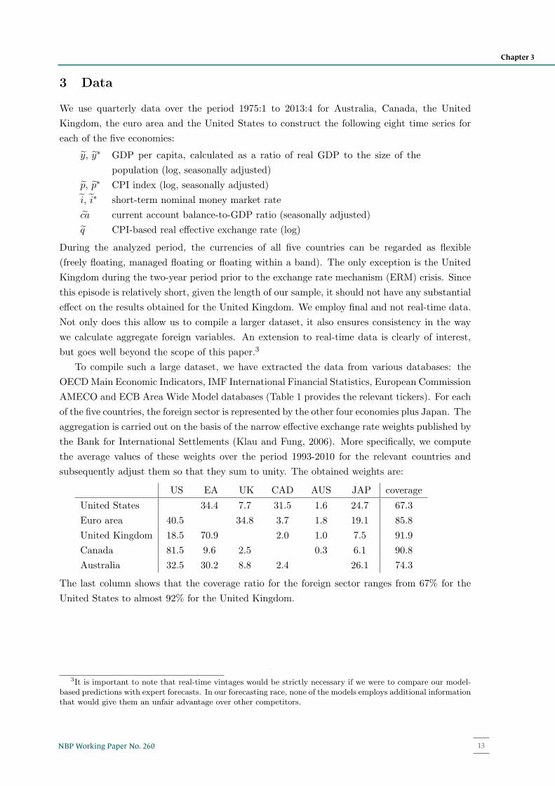
subsequently adjust them so that they sum to unity. The obtained weights are:
US EA UK CAD AUS JAP coverage
United States 34.4 7.7 31.5 1.6 24.7 67.3
Euro area 40.5 34.8 3.7 1.8 19.1 85.8
United Kingdom 18.5 70.9 2.0 1.0 7.5 91.9
Canada 81.5 9.6 2.5 0.3 6.1 90.8
Australia 32.5 30.2 8.8 2.4 26.1 74.3
The last column shows that the coverage ratio for the foreign sector ranges from 67% for the
United States to almost 92% for the United Kingdom.
3It is important to note that real-time vintages would be strictly necessary if we were to compare our model-based predictions with expert forecasts. In our forecasting race, none of the models employs additional informationthat would give them an unfair advantage over other competitors.
13
any value in this range, which is consistent with the results of Ca’ Zorzi et al. (2016).
3 Data
We use quarterly data over the period 1975:1 to 2013:4 for Australia, Canada, the United
Kingdom, the euro area and the United States to construct the following eight time series for
each of the five economies:
y, y∗ GDP per capita, calculated as a ratio of real GDP to the size of the
population (log, seasonally adjusted)
p, p∗ CPI index (log, seasonally adjusted)
i, i∗ short-term nominal money market rate
ca current account balance-to-GDP ratio (seasonally adjusted)
q CPI-based real effective exchange rate (log)
During the analyzed period, the currencies of all five countries can be regarded as flexible
(freely floating, managed floating or floating within a band). The only exception is the United
Kingdom during the two-year period prior to the exchange rate mechanism (ERM) crisis. Since
this episode is relatively short, given the length of our sample, it should not have any substantial
effect on the results obtained for the United Kingdom. We employ final and not real-time data.
Not only does this allow us to compile a larger dataset, it also ensures consistency in the way
we calculate aggregate foreign variables. An extension to real-time data is clearly of interest,
but goes well beyond the scope of this paper.3
To compile such a large dataset, we have extracted the data from various databases: the
OECDMain Economic Indicators, IMF International Financial Statistics, European Commission
AMECO and ECB Area Wide Model databases (Table 1 provides the relevant tickers). For each
of the five countries, the foreign sector is represented by the other four economies plus Japan. The
aggregation is carried out on the basis of the narrow effective exchange rate weights published by
the Bank for International Settlements (Klau and Fung, 2006). More specifically, we compute
the average values of these weights over the period 1993-2010 for the relevant countries and
subsequently adjust them so that they sum to unity. The obtained weights are:
US EA UK CAD AUS JAP coverage
United States 34.4 7.7 31.5 1.6 24.7 67.3
Euro area 40.5 34.8 3.7 1.8 19.1 85.8
United Kingdom 18.5 70.9 2.0 1.0 7.5 91.9
Canada 81.5 9.6 2.5 0.3 6.1 90.8
Australia 32.5 30.2 8.8 2.4 26.1 74.3
The last column shows that the coverage ratio for the foreign sector ranges from 67% for the
United States to almost 92% for the United Kingdom.
3It is important to note that real-time vintages would be strictly necessary if we were to compare our model-based predictions with expert forecasts. In our forecasting race, none of the models employs additional informationthat would give them an unfair advantage over other competitors.
13
13NBP Working Paper No. 260
Chapter 3
y, y∗, p, p∗, i, i∗, ca and q as observables), another one with some of the variables expressed
in “differences” (DBVAR, for ∆y, ∆y∗, ∆p, ∆p∗, i, i∗, ca and ∆q), and yet another one where
we exploit the methodology of Villani (2009) to elicit the prior that the RER is mean reverting
(MBVAR, for ∆y, ∆y∗, ∆p, ∆p∗, i, i∗, ca and q). In all cases we use the specification with four
lags as the models are fitted to the data of quarterly frequency.
As regards the details of the estimation process, we use the standard Normal-Wishart prior
proposed by Kadiyala and Karlsson (1997) for LBVAR and DBVAR models, and assume a
normal-diffuse prior for the MBVAR as in Villani (2009). For the model in levels (LBVAR), we
use the standard RW prior. For the mixed models (MBVAR and DBVAR), we follow Adolf-
son et al. (2007b) and Villani (2009), centering the prior for the first own lag at zero for the
differenced variables and at 0.9 for the variables in levels. The prior mean for all other VAR
coefficients are set to zero. As regards the dispersion of the prior distributions, we assume that
they are tighter for higher lags (decay hyperparameter is set to 1) and choose the conventional
value of 0.2 for the overall tightness hyperparameter. In the case of the MBVAR model, we
additionally set the prior variance for cross-variable coefficients to lower values than for their
own lags (weight hyperparameter equal to 0.5). The steady-state prior for the RER is centered
at its recursive mean, with tightness such that the 95% interval coincides with the 2.5% range
around this mean. As regards the remaining economic variables, we take standard values sug-
gested by the literature. The 95% interval is defined as 0.5% 0.25% for steady-state (quarterly)
inflation and output growth, 1.0% 0.25% for the (quarterly) interest rate, and 0% 1.5% for
the current account to GDP ratio.
Atheoretical benchmarks
We also include two atheoretical models into the race. The first one is the most widely used
benchmark in the exchange rate forecasting literature, i.e. the naıve RW model. From the
perspective of a forecasting practitioner, there is nothing more conservative than assuming that
no changes occur over the forecast horizon. We also propose another atheoretical model, which
practitioners all know very well and which consists in simply assuming that the variable of
interest gradually returns to its average past value. Since in this method the parameter that
determines the speed of convergence to the mean is calibrated by the modeler, we label it as
AR-fixed. This method was recently shown by Faust and Wright (2013) to be very competitive
relative to several other forecasting schemes for inflation and by Ca’ Zorzi et al. (2016) for
the RER. More generally, this illustrates that a reasonable gliding path between two good
boundary values, one for the starting point and one for the long-term value, performs well in
forecasting. The AR-fixed model shares with the RW the convenient feature that it is not subject
to estimation error. At the same time, it is more appealing than the RW as, consistently with
the macro literature, it foresees that the RER is mean reverting.
In the empirical application we set the autoregressive parameter of the AR-fixed model to
0.95, which is consistent with the half-life adjustment of just over three years. This is within
the range between three and five years suggested by Rogoff (1996) in his influential survey on
the persistence of the RER. However, the analysis that we present in this article is robust to
12
any value in this range, which is consistent with the results of Ca’ Zorzi et al. (2016).
3 Data
We use quarterly data over the period 1975:1 to 2013:4 for Australia, Canada, the United
Kingdom, the euro area and the United States to construct the following eight time series for
each of the five economies:
y, y∗ GDP per capita, calculated as a ratio of real GDP to the size of the
population (log, seasonally adjusted)
p, p∗ CPI index (log, seasonally adjusted)
i, i∗ short-term nominal money market rate
ca current account balance-to-GDP ratio (seasonally adjusted)
q CPI-based real effective exchange rate (log)
During the analyzed period, the currencies of all five countries can be regarded as flexible
(freely floating, managed floating or floating within a band). The only exception is the United
Kingdom during the two-year period prior to the exchange rate mechanism (ERM) crisis. Since
this episode is relatively short, given the length of our sample, it should not have any substantial
effect on the results obtained for the United Kingdom. We employ final and not real-time data.
Not only does this allow us to compile a larger dataset, it also ensures consistency in the way
we calculate aggregate foreign variables. An extension to real-time data is clearly of interest,
but goes well beyond the scope of this paper.3
To compile such a large dataset, we have extracted the data from various databases: the
OECDMain Economic Indicators, IMF International Financial Statistics, European Commission
AMECO and ECB Area Wide Model databases (Table 1 provides the relevant tickers). For each
of the five countries, the foreign sector is represented by the other four economies plus Japan. The
aggregation is carried out on the basis of the narrow effective exchange rate weights published by
the Bank for International Settlements (Klau and Fung, 2006). More specifically, we compute
the average values of these weights over the period 1993-2010 for the relevant countries and
subsequently adjust them so that they sum to unity. The obtained weights are:
US EA UK CAD AUS JAP coverage
United States 34.4 7.7 31.5 1.6 24.7 67.3
Euro area 40.5 34.8 3.7 1.8 19.1 85.8
United Kingdom 18.5 70.9 2.0 1.0 7.5 91.9
Canada 81.5 9.6 2.5 0.3 6.1 90.8
Australia 32.5 30.2 8.8 2.4 26.1 74.3
The last column shows that the coverage ratio for the foreign sector ranges from 67% for the
United States to almost 92% for the United Kingdom.
3It is important to note that real-time vintages would be strictly necessary if we were to compare our model-based predictions with expert forecasts. In our forecasting race, none of the models employs additional informationthat would give them an unfair advantage over other competitors.
13

Narodowy Bank Polski14
Chapter 4
4 Results for the real exchange rate
We assess the out-of-sample forecast performance of the baseline DSGE model and its competi-
tors for horizons ranging from one quarter to six years. The models are estimated using recursive
samples.4 The point forecasts were calculated as the means of draws from each model’s pre-
dictive density. Note that generating the forecasts for DSGE models alone required running
estimation, performing convergence checks and drawing from the predictive density 760 times
(since we have 76 different estimation windows for each country and two DSGE variants). The
total computer time needed to execute all these steps amounted to almost half a year.5
Forecast accuracy
We begin our analysis by measuring the forecasting performance of the seven competing methods
with the root mean squared forecast errors (RMSFEs) for the RER (Table 2). We report the
RMSFE values as ratios in comparison to the RW, so that values below unity indicate that
a given model outperforms the no-change benchmark. We also test the null of equal forecast
accuracy with the two-sided Diebold-Mariano test.
A number of key features of the results are immediately evident. The AR-fixed, MBVAR
and baseline DSGE models have generally the lowest RMSFEs at longer horizons. They over-
whelmingly beat the RW for the United States, the euro area and the United Kingdom, while
the results are broadly similar for Australia and Canada. Of the two DSGE models, the baseline
version (without trend in RER) is consistently better than the alternative (with trend). This
indicates that attempts to explain in-sample low frequency movements in the RER are coun-
terproductive out of sample. Of the three BVAR models, the MBVAR is the most accurate,
followed by LBVAR and, at a considerable distance, DBVAR. This suggests that differencing
the RER before estimation attributes too much weight to short-term dynamics. It also reveals
that setting an informative prior for the long-run level of the RER enhances the out-of-sample
performance of BVAR models.
To shed some light on the absolute performance of the competing models, we run the so-
called Mincer-Zarnowitz regressions. This consists in regressing the realized values of the RER
qt+h on a constant and their h-step ahead forecasts qft+h:
qt+h = α+ βqft+h + ηt+h. (1)
For an efficient forecasting model, the constant term should be zero, the slope coefficient unity
and the fit of the regression measured by the R2 coefficient high. Table 3 reports the outcomes
for the shortest (one-quarter-ahead) and longest (six-years-ahead) horizons considered in this
paper. It presents the parameter estimates for α and β, the R2 coefficient and the p-value of
4For each country, the one-quarter-ahead forecasts are evaluated on the basis of 76 observations, two-quarter-ahead forecasts on the basis of 75 observations, and so forth with the 24-quarter-ahead forecasts comprising53 observations. The first set of forecasts is elaborated with models estimated over the sample 1975:1-1994:4for the period 1995:1-2000:4. This procedure is repeated with samples ending in each quarter from the period1995:2-2013:3.
5We used the Intel(R) Xeon(R) 3.40GHz Processor.
14
the joint test that α = 0 and β = 1. At the one-quarter horizon, the null of forecast efficiency
cannot be rejected at the 5% significance level in almost all cases for the AR-fixed, baseline
DSGE and MBVAR models. The third criterion required to establish efficiency is however not
fulfiled as the R2 never exceeds 5%. At the six-year horizon, where the fit of the regressions is
much higher, the null of efficiency is rejected almost always for all models. In terms of efficiency,
all models disappoint, even if to a different degree.
The results of the Mincer-Zarnowitz regressions are also illustrated graphically in Figures
1 and 2, which present scatter plots of the RER realizations (y-axis) versus the model-based
forecasts (x-axis). Points along the 45 degree line correspond to perfect predictions, i.e. the
maximum degree of efficiency possible. Observations that fall in the top-right and bottom-left
quadrants are forecasts that anticipate correctly the directional change of the RER. Based on
their position relative to the 45 degree line, the predictions that have the correct sign can be
further split between those where the forecasted absolute change in the RER is larger (overpre-
diction) or smaller (underprediction) than the realization. Table 4 provides a set of indicators
that summarize the information in the scatter plots. In the upper panel we present the per-
centage of forecasts that have the correct sign. This is complemented by the goodness-of-fit χ2
test to evaluate if this number is significantly different from 50% (Pesaran and Timmermann,
1992). In the second panel we show the percentage of forecasts that underpredict the realized
values. The third panel reports the correlation coefficients between forecasts and actual data.
The fourth and final panel contains an indicator that we label as “relative volatility” as it mea-
sures the ratio of the average absolute forecasted change in the RER to the average absolute
actual change in this variable. The value of this indicator is by definition zero for the RW (very
conservative) and 100% for the perfect model.
The findings of both Figure 1 and the left columns of Table 4 confirm that at a short horizon
none of the models perform particularly well. Most observations are distant from the 45 degree
line, correlation is low and the share of forecasts that have the correct sign is almost never
significantly different from 50%. At longer horizons the AR-fixed, MBVAR and baseline DSGE
models prove to be much better than the competition. Albeit not perfectly aligned along the
45 degree line (Figure 2), most observations can be found in the “correct” quadrants, i.e. the
top-right and bottom-left ones. For example, the euro forecasts are of the correct sign in about
70% of cases with the AR-fixed and MBVAR models and in almost 80% with the baseline DSGE
model (right columns of Table 4). In these three models the null of a random draw equal to
50% is strongly rejected at the 1% significance level for all countries except Australia. Our three
best-performing models also generate forecasts that are highly and positively correlated with
actual data for all currencies but the Australian dollar. The right columns of Table 4 also show
that these models have a strong tendency to underpredict the absolute size of RER movements,
which is reflected in the “relative volatility” indicator having values that are much lower than
100%. The only model that is able to describe well the scale of future fluctuations in the RER
is DBVAR, but typically its forecast goes in the wrong direction. To sum up, the scatter plots
and statistics discussed above confirm that the AR-fixed, MBVAR and baseline DSGE models
are the most accurate, especially at longer horizons.
15
15NBP Working Paper No. 260
Results for the real exchange rate
4 Results for the real exchange rate
We assess the out-of-sample forecast performance of the baseline DSGE model and its competi-
tors for horizons ranging from one quarter to six years. The models are estimated using recursive
samples.4 The point forecasts were calculated as the means of draws from each model’s pre-
dictive density. Note that generating the forecasts for DSGE models alone required running
estimation, performing convergence checks and drawing from the predictive density 760 times
(since we have 76 different estimation windows for each country and two DSGE variants). The
total computer time needed to execute all these steps amounted to almost half a year.5
Forecast accuracy
We begin our analysis by measuring the forecasting performance of the seven competing methods
with the root mean squared forecast errors (RMSFEs) for the RER (Table 2). We report the
RMSFE values as ratios in comparison to the RW, so that values below unity indicate that
a given model outperforms the no-change benchmark. We also test the null of equal forecast
accuracy with the two-sided Diebold-Mariano test.
A number of key features of the results are immediately evident. The AR-fixed, MBVAR
and baseline DSGE models have generally the lowest RMSFEs at longer horizons. They over-
whelmingly beat the RW for the United States, the euro area and the United Kingdom, while
the results are broadly similar for Australia and Canada. Of the two DSGE models, the baseline
version (without trend in RER) is consistently better than the alternative (with trend). This
indicates that attempts to explain in-sample low frequency movements in the RER are coun-
terproductive out of sample. Of the three BVAR models, the MBVAR is the most accurate,
followed by LBVAR and, at a considerable distance, DBVAR. This suggests that differencing
the RER before estimation attributes too much weight to short-term dynamics. It also reveals
that setting an informative prior for the long-run level of the RER enhances the out-of-sample
performance of BVAR models.
To shed some light on the absolute performance of the competing models, we run the so-
called Mincer-Zarnowitz regressions. This consists in regressing the realized values of the RER
qt+h on a constant and their h-step ahead forecasts qft+h:
qt+h = α+ βqft+h + ηt+h. (1)
For an efficient forecasting model, the constant term should be zero, the slope coefficient unity
and the fit of the regression measured by the R2 coefficient high. Table 3 reports the outcomes
for the shortest (one-quarter-ahead) and longest (six-years-ahead) horizons considered in this
paper. It presents the parameter estimates for α and β, the R2 coefficient and the p-value of
4For each country, the one-quarter-ahead forecasts are evaluated on the basis of 76 observations, two-quarter-ahead forecasts on the basis of 75 observations, and so forth with the 24-quarter-ahead forecasts comprising53 observations. The first set of forecasts is elaborated with models estimated over the sample 1975:1-1994:4for the period 1995:1-2000:4. This procedure is repeated with samples ending in each quarter from the period1995:2-2013:3.
5We used the Intel(R) Xeon(R) 3.40GHz Processor.
14
the joint test that α = 0 and β = 1. At the one-quarter horizon, the null of forecast efficiency
cannot be rejected at the 5% significance level in almost all cases for the AR-fixed, baseline
DSGE and MBVAR models. The third criterion required to establish efficiency is however not
fulfiled as the R2 never exceeds 5%. At the six-year horizon, where the fit of the regressions is
much higher, the null of efficiency is rejected almost always for all models. In terms of efficiency,
all models disappoint, even if to a different degree.
The results of the Mincer-Zarnowitz regressions are also illustrated graphically in Figures
1 and 2, which present scatter plots of the RER realizations (y-axis) versus the model-based
forecasts (x-axis). Points along the 45 degree line correspond to perfect predictions, i.e. the
maximum degree of efficiency possible. Observations that fall in the top-right and bottom-left
quadrants are forecasts that anticipate correctly the directional change of the RER. Based on
their position relative to the 45 degree line, the predictions that have the correct sign can be
further split between those where the forecasted absolute change in the RER is larger (overpre-
diction) or smaller (underprediction) than the realization. Table 4 provides a set of indicators
that summarize the information in the scatter plots. In the upper panel we present the per-
centage of forecasts that have the correct sign. This is complemented by the goodness-of-fit χ2
test to evaluate if this number is significantly different from 50% (Pesaran and Timmermann,
1992). In the second panel we show the percentage of forecasts that underpredict the realized
values. The third panel reports the correlation coefficients between forecasts and actual data.
The fourth and final panel contains an indicator that we label as “relative volatility” as it mea-
sures the ratio of the average absolute forecasted change in the RER to the average absolute
actual change in this variable. The value of this indicator is by definition zero for the RW (very
conservative) and 100% for the perfect model.
The findings of both Figure 1 and the left columns of Table 4 confirm that at a short horizon
none of the models perform particularly well. Most observations are distant from the 45 degree
line, correlation is low and the share of forecasts that have the correct sign is almost never
significantly different from 50%. At longer horizons the AR-fixed, MBVAR and baseline DSGE
models prove to be much better than the competition. Albeit not perfectly aligned along the
45 degree line (Figure 2), most observations can be found in the “correct” quadrants, i.e. the
top-right and bottom-left ones. For example, the euro forecasts are of the correct sign in about
70% of cases with the AR-fixed and MBVAR models and in almost 80% with the baseline DSGE
model (right columns of Table 4). In these three models the null of a random draw equal to
50% is strongly rejected at the 1% significance level for all countries except Australia. Our three
best-performing models also generate forecasts that are highly and positively correlated with
actual data for all currencies but the Australian dollar. The right columns of Table 4 also show
that these models have a strong tendency to underpredict the absolute size of RER movements,
which is reflected in the “relative volatility” indicator having values that are much lower than
100%. The only model that is able to describe well the scale of future fluctuations in the RER
is DBVAR, but typically its forecast goes in the wrong direction. To sum up, the scatter plots
and statistics discussed above confirm that the AR-fixed, MBVAR and baseline DSGE models
are the most accurate, especially at longer horizons.
15
Narodowy Bank Polski16
The anatomy of the results
In what follows we investigate what is driving the results reported above. A good way forward
is to get a visual impression of the performance of the six models by plotting the whole sequence
of forecasts for the RER, conducted at different points in time, and comparing them to the
actuals (Figure 3). A first inspection suggests that the baseline DSGE and AR-fixed models
are characterized by conservative forecasts, i.e. forecasts that do not attempt to explain a large
fraction of the data variation or to anticipate the turning points. The charts also show that for
the baseline DSGE, MBVAR and AR-fixed models there is a visible mean-reversion mechanism.
Conversely, the worst performing model in terms of the RMSFE, i.e. the DBVAR model, delivers
forecasts which very often stray away from the mean in a way that is strongly influenced by
developments that briefly precede the forecast formulation. The LBVAR and DSGE (with trend
in the RER) models extrapolate long-term trends rather than project their correction; hence their
forecast accuracy for longer horizons is relatively low. Among the three mean-reverting methods,
the MBVAR model has the richest short-term dynamics, but this harms rather than enhances its
performance. It is clear that in our forecasting race the conservatism of the DSGE and AR-fixed
models, which also manifests itself in the low “relative volatility” indicators reported in Table 4,
shields them from incurring large forecast errors. Among the three BVAR models, the MBVAR
is the least erratic and best performing. This is intuitive since the steady-state priors anchor its
short-term forecasts within a reasonable range.
Some simple statistics help us to gauge better what role mean reversion plays in the data
and how well it is captured by our forecasting tools. We start by counting how many times the
RER moves toward its recursive mean. These numbers can be found in the last rows of each
country panel in Table 5. They reveal that at shorter horizons, e.g. one year ahead, there is no
evidence of mean reversion or diversion. At the lowest end of the range we find the euro area,
where the RER reverts towards its mean only 45% of the times. At the highest end we find
the United Kingdom, for which mean reversion takes place in 71% of the cases. The number
of episodes where the RER moves towards its mean tends to increase monotonically with the
length of the forecast horizon. After 24 quarters, this frequency is in the range between 64% for
Canada and 89% for the United Kingdom. The only notable exception is Australia, where the
indicator cannot pick up any evidence of mean reversion either in the short or long term.
It may be nonetheless misleading to just count the episodes of mean reversion without
evaluating the strength of the correction. To explore this issue in greater depth, for each model,
currency and forecast horizon we calculate the following statistics to measure the pace of mean
reversion (PMR):
PMRh = −100T∑t=1
wt
qft+h − qt
qt − qt, (2)
where qft+h is an h-step-ahead forecast for the RER elaborated at period t, qt is the recursive mean
for observations up to time t and wt indicates a weight that is proportional to the deviation of
the RER from the recursive mean, i.e. wt = |qt−qt|/∑T
t=1 |qt−qt|. The reason for this weighting
16
scheme is that, for small deviations from the steady state, the mean-reverting forces are likely
to be obscured by other short-term factors. Positive values of the PMR statistics point to mean
reversion and negative ones to mean divergence. If a model predicts the full return to the sample
mean within a given horizon, then PMR = 100. Given the above definition, this statistic will
be equal to zero for the RW benchmark at all horizons. For the AR-fixed model, the equation
can be derived analytically, namely PMRh = 100× (1− 0.95h). For the remaining models the
PMR statistic is calculated numerally using point forecasts.6
The PMR values for the six models in our forecasting race are presented in the first six rows
of each country panel in Table 5. The seventh row shows the corresponding statistics for realized
data. It is insightful to look at the realized data first. The PMR indicator reveals that, contrary
to the common presumption, mean reversion already starts at short horizons, even if very feebly.
For example, the pace of convergence of the RER for the euro towards its mean increases from
less than 10% at the end of the first year to 30% after three years; it then accelerates, reaching
120% by the end of our forecast horizon. This suggests that at long horizons there are a few
important episodes where the adjustment even overshot what was predicted by the relative PPP.
The table also shows that an entirely analogous adjustment characterizes the US dollar and the
British pound. A steady rise in the forces of mean reversion is also detectable for the Canadian
dollar, but the correction is incomplete even after six years. Finally, the evidence of mean
reversion is again almost non-existent for the Australian dollar, except at very long horizons.
The PMR indicator for our best three models, i.e. the AR-fixed, MBVAR and baseline
DSGE, matches the data rather well. They correctly anticipate that mean reversion plays
initially a minor role but eventually becomes more important. This helps us to get a grasp of
why these models, in particular AR-fixed, are already competitive at short forecasting horizons
and become increasingly harder to beat at longer horizons. The other models instead miss this
opportunity. The DBVAR model generally predicts mean divergence both for short-term and
long-term horizons. A similar story can be told for the LBVAR model for Canada and Australia.
To sum up, the failure of the standard BVARs to account for the mean-reverting property in the
data is consistent with their poor forecasting performance. It is also worth noting that even for
Australia, where the evidence of mean reversion is weaker, our benchmark DSGE clearly beats
its “twin” variant (with trend) in terms of RMSFEs.
Equilibrium exchange rates
In the previous subsection we have shown that the best forecasting models are capable of repli-
cating the mean reversion in the RER observed in the data. It should be noted, however, that
the “end-point” is not the same across models. In the case of the AR- fixed model it is equal to
the recursive mean, while for the MBVAR and DSGE models it is the model-based steady-state
of the RER. It is natural to interpret these “end-points” as proxies for the long-run equilibrium
exchange rate, which is consistent with PPP. There is however a bewildering plethora of different
6An alternative to calculating PMR could be to run a regression qft+h − qt = γ(qt − qt) + εt+h. This was doneby Eichenbaum et al. (2017), who showed that the estimates of γ for longer horizons are close to unity for mostflexible exchange rate countries, which is also consistent with their DSGE model.
17
17NBP Working Paper No. 260
Results for the real exchange rate
The anatomy of the results
In what follows we investigate what is driving the results reported above. A good way forward
is to get a visual impression of the performance of the six models by plotting the whole sequence
of forecasts for the RER, conducted at different points in time, and comparing them to the
actuals (Figure 3). A first inspection suggests that the baseline DSGE and AR-fixed models
are characterized by conservative forecasts, i.e. forecasts that do not attempt to explain a large
fraction of the data variation or to anticipate the turning points. The charts also show that for
the baseline DSGE, MBVAR and AR-fixed models there is a visible mean-reversion mechanism.
Conversely, the worst performing model in terms of the RMSFE, i.e. the DBVAR model, delivers
forecasts which very often stray away from the mean in a way that is strongly influenced by
developments that briefly precede the forecast formulation. The LBVAR and DSGE (with trend
in the RER) models extrapolate long-term trends rather than project their correction; hence their
forecast accuracy for longer horizons is relatively low. Among the three mean-reverting methods,
the MBVAR model has the richest short-term dynamics, but this harms rather than enhances its
performance. It is clear that in our forecasting race the conservatism of the DSGE and AR-fixed
models, which also manifests itself in the low “relative volatility” indicators reported in Table 4,
shields them from incurring large forecast errors. Among the three BVAR models, the MBVAR
is the least erratic and best performing. This is intuitive since the steady-state priors anchor its
short-term forecasts within a reasonable range.
Some simple statistics help us to gauge better what role mean reversion plays in the data
and how well it is captured by our forecasting tools. We start by counting how many times the
RER moves toward its recursive mean. These numbers can be found in the last rows of each
country panel in Table 5. They reveal that at shorter horizons, e.g. one year ahead, there is no
evidence of mean reversion or diversion. At the lowest end of the range we find the euro area,
where the RER reverts towards its mean only 45% of the times. At the highest end we find
the United Kingdom, for which mean reversion takes place in 71% of the cases. The number
of episodes where the RER moves towards its mean tends to increase monotonically with the
length of the forecast horizon. After 24 quarters, this frequency is in the range between 64% for
Canada and 89% for the United Kingdom. The only notable exception is Australia, where the
indicator cannot pick up any evidence of mean reversion either in the short or long term.
It may be nonetheless misleading to just count the episodes of mean reversion without
evaluating the strength of the correction. To explore this issue in greater depth, for each model,
currency and forecast horizon we calculate the following statistics to measure the pace of mean
reversion (PMR):
PMRh = −100T∑t=1
wt
qft+h − qt
qt − qt, (2)
where qft+h is an h-step-ahead forecast for the RER elaborated at period t, qt is the recursive mean
for observations up to time t and wt indicates a weight that is proportional to the deviation of
the RER from the recursive mean, i.e. wt = |qt−qt|/∑T
t=1 |qt−qt|. The reason for this weighting
16
scheme is that, for small deviations from the steady state, the mean-reverting forces are likely
to be obscured by other short-term factors. Positive values of the PMR statistics point to mean
reversion and negative ones to mean divergence. If a model predicts the full return to the sample
mean within a given horizon, then PMR = 100. Given the above definition, this statistic will
be equal to zero for the RW benchmark at all horizons. For the AR-fixed model, the equation
can be derived analytically, namely PMRh = 100× (1− 0.95h). For the remaining models the
PMR statistic is calculated numerally using point forecasts.6
The PMR values for the six models in our forecasting race are presented in the first six rows
of each country panel in Table 5. The seventh row shows the corresponding statistics for realized
data. It is insightful to look at the realized data first. The PMR indicator reveals that, contrary
to the common presumption, mean reversion already starts at short horizons, even if very feebly.
For example, the pace of convergence of the RER for the euro towards its mean increases from
less than 10% at the end of the first year to 30% after three years; it then accelerates, reaching
120% by the end of our forecast horizon. This suggests that at long horizons there are a few
important episodes where the adjustment even overshot what was predicted by the relative PPP.
The table also shows that an entirely analogous adjustment characterizes the US dollar and the
British pound. A steady rise in the forces of mean reversion is also detectable for the Canadian
dollar, but the correction is incomplete even after six years. Finally, the evidence of mean
reversion is again almost non-existent for the Australian dollar, except at very long horizons.
The PMR indicator for our best three models, i.e. the AR-fixed, MBVAR and baseline
DSGE, matches the data rather well. They correctly anticipate that mean reversion plays
initially a minor role but eventually becomes more important. This helps us to get a grasp of
why these models, in particular AR-fixed, are already competitive at short forecasting horizons
and become increasingly harder to beat at longer horizons. The other models instead miss this
opportunity. The DBVAR model generally predicts mean divergence both for short-term and
long-term horizons. A similar story can be told for the LBVAR model for Canada and Australia.
To sum up, the failure of the standard BVARs to account for the mean-reverting property in the
data is consistent with their poor forecasting performance. It is also worth noting that even for
Australia, where the evidence of mean reversion is weaker, our benchmark DSGE clearly beats
its “twin” variant (with trend) in terms of RMSFEs.
Equilibrium exchange rates
In the previous subsection we have shown that the best forecasting models are capable of repli-
cating the mean reversion in the RER observed in the data. It should be noted, however, that
the “end-point” is not the same across models. In the case of the AR- fixed model it is equal to
the recursive mean, while for the MBVAR and DSGE models it is the model-based steady-state
of the RER. It is natural to interpret these “end-points” as proxies for the long-run equilibrium
exchange rate, which is consistent with PPP. There is however a bewildering plethora of different
6An alternative to calculating PMR could be to run a regression qft+h − qt = γ(qt − qt) + εt+h. This was doneby Eichenbaum et al. (2017), who showed that the estimates of γ for longer horizons are close to unity for mostflexible exchange rate countries, which is also consistent with their DSGE model.
17
Narodowy Bank Polski18
equilibrium exchange rate concepts in the literature, which relate to shorter horizons than PPP
(Bussiere et al., 2010). In relation to this literature, the DSGE model incorporates a stock-flow
adjustment mechanism that is consistent with the Fundamental Equilibrium Exchange Rate
approach. Over medium-term horizons, large imbalances in net foreign assets require current
account deficits or surpluses, which imply prolonged RER deviations from the steady-state. The
model also incorporates some features of the behavioral equilibrium exchange rate framework
as, over short horizons, the RER deviates from the steady-state in the case of differences in the
restrictiveness of monetary policy.
To see how much these theoretical differences matter empirically, we plot in Figure 4 the
recursive estimates of the equilibrium RER for all three models. It can be seen that the estimates
from the AR-fixed and MBVAR models are almost the same. Although in the latter case relative
PPP is only set as a long-run prior, the outcome is almost identical to the recursive mean. The
differences between the recursive mean of the RER and the steady-state RER implied by the
DSGE model are instead typically larger. The average absolute distance between them varies
between 0.7% for Australia and 2.8% for the euro area. There are, however, specific cases where
the gap is much larger. For example, in the years after the euro was launched, the US dollar rose
significantly against the euro. A retrospective look at that episode tells us that in the period
1999-2003 the real effective exchange rate of the dollar was (on average) overvalued by 11%
according to the AR-fixed and MBVAR models, but only by 3% according to the DSGE model.
The DSGEmodel-based concept of equilibrium exchange rate is particularly appealing thanks
to the strong theoretical foundations of the model. It guarantees both a mean-reversion mecha-
nism for the RER and long-term current account sustainability. However, the estimated equilib-
rium exchange rate is more volatile than that implied by the other two models. There are various
cases where adding just one observation to the estimation sample leads to a re-assessment of the
equilibrium exchange rate by more than 10%. We interpret this result as a sign of the sizable
role of estimation error. This feature clearly puts the DSGE model at a disadvantage relative to
the other two models, which instead reassess the arrival of new information only marginally and
hence avoid picking up spurious in-sample dynamics (Faust and Wright, 2013). The equilibrium
exchange rate calculated with the AR-fixed or MBVAR model therefore has weaker theoretical
foundations, but is more stable.
Adjustment dynamics
Our three preferred models also feature different dynamic adjustments to their respective steady
states. In particular, Figure 5 illustrates how the long-run equilibrium is restored in the AR-fixed
and DSGE models. In the former case, this adjustment is just a simple log-linear gliding path
towards the historical mean. In the latter case, the path of adjustment is more complex as it
depends on the dynamic reactions of the RER to eight different disturbances and the historical
realizations of the shocks. For example, if the RER is tilted from its steady state by a monetary
shock, the return to the equilibrium is rapid. By contrast, it takes many years to eliminate
the impact of an import cost-push shock. Moreover, the shapes of the impulse responses do
not always point to a gradual return to the steady state, as they sometimes have an oscillating
18
pattern, as for example in the aftermath of shocks affecting foreign variables. The impulse
response functions presented in Figure 5 also help us explain the cross-country differences in
mean reversion implied by the DSGE model. It is clear that the effects of a cost-push shock,
which accounts for the bulk of RER fluctuations, especially at medium and long horizons, are
more persistent for the United States and Australia than for the United Kingdom and Canada,
which is consistent with the statistics reported in Table 5.
In comparison to the AR-fixed model, the DSGE framework is naturally richer since it
provides forecasts that can be both time variant and country specific. In particular, there are
episodes where the RER initially diverges further from the steady state in order to bring the
current account back on a converging path towards its steady state. For instance, this is the case
for the US dollar RER forecast elaborated with data ending in the third quarter of 2013. Even
though the DSGE model interprets the RER as undervalued by 5.6% relative to the long-term
equilibrium, it predicts a further depreciation by 3.5% over a six-year horizon. The reason is
that, according to the model, this depreciation was required to repay the US net foreign debt,
which had been accumulated by persistent current account deficits in the past.
The fundamental question is whether this kind of structural macroeconomic argument gives
the DSGE model a forecasting edge over atheoretical benchmarks such as the AR-fixed or MB-
VAR models. We have already seen that, in terms of the RMSFE, the forecasting performance
of the three models tends to be quite similar. However, if we go back to Table 4, we can notice
that the DSGE model does a much better job at capturing the direction of the RER movements
over longer horizons. This suggests that the macroeconomic mechanisms embedded in the DSGE
framework, by allowing for time and country variation in the speed of mean reversion of the
RER, tend to improve the quality of the forecasts for this variable. This result is remarkable
considering that the DSGE model is subject to estimation error and is more sensitive to spu-
rious in-sample dynamics than the calibrated AR-fixed benchmark. Naturally, there are also
other, more practical considerations that may affect the choice between these three competing
forecasting methods. The strength of the AR-fixed and, to some extent, the MBVAR model is
their simplicity and tractability. The comparative advantage of the DSGE model is that it is
able to provide a consistent macroeconomic explanation of adjustment to the equilibrium, not
only for the RER, but also for a wider set of economic variables.
5 Results for the nominal exchange rate
A lifetime ambition of many exchange rate economists is to develop a fully-fledged macro model
that helps forecasting the nominal and not just the real exchange rate. It is hence natural to ask
if the predictability that we have identified for the RER extends to the NER. To assess whether
this is the case, we keep in the race, in addition to the RW, only two competitors, i.e. the
baseline DSGE and MBVAR models. Our choice is motivated by their good performance for the
RER matched by their ability to deliver separate forecasts for the NER and the relative price
index (RPI), the latter being defined as the ratio of domestic and foreign consumer price indices.
The results, however, are disappointing as both models fail to beat the RW systematically in
19
19NBP Working Paper No. 260
Chapter 5
equilibrium exchange rate concepts in the literature, which relate to shorter horizons than PPP
(Bussiere et al., 2010). In relation to this literature, the DSGE model incorporates a stock-flow
adjustment mechanism that is consistent with the Fundamental Equilibrium Exchange Rate
approach. Over medium-term horizons, large imbalances in net foreign assets require current
account deficits or surpluses, which imply prolonged RER deviations from the steady-state. The
model also incorporates some features of the behavioral equilibrium exchange rate framework
as, over short horizons, the RER deviates from the steady-state in the case of differences in the
restrictiveness of monetary policy.
To see how much these theoretical differences matter empirically, we plot in Figure 4 the
recursive estimates of the equilibrium RER for all three models. It can be seen that the estimates
from the AR-fixed and MBVAR models are almost the same. Although in the latter case relative
PPP is only set as a long-run prior, the outcome is almost identical to the recursive mean. The
differences between the recursive mean of the RER and the steady-state RER implied by the
DSGE model are instead typically larger. The average absolute distance between them varies
between 0.7% for Australia and 2.8% for the euro area. There are, however, specific cases where
the gap is much larger. For example, in the years after the euro was launched, the US dollar rose
significantly against the euro. A retrospective look at that episode tells us that in the period
1999-2003 the real effective exchange rate of the dollar was (on average) overvalued by 11%
according to the AR-fixed and MBVAR models, but only by 3% according to the DSGE model.
The DSGEmodel-based concept of equilibrium exchange rate is particularly appealing thanks
to the strong theoretical foundations of the model. It guarantees both a mean-reversion mecha-
nism for the RER and long-term current account sustainability. However, the estimated equilib-
rium exchange rate is more volatile than that implied by the other two models. There are various
cases where adding just one observation to the estimation sample leads to a re-assessment of the
equilibrium exchange rate by more than 10%. We interpret this result as a sign of the sizable
role of estimation error. This feature clearly puts the DSGE model at a disadvantage relative to
the other two models, which instead reassess the arrival of new information only marginally and
hence avoid picking up spurious in-sample dynamics (Faust and Wright, 2013). The equilibrium
exchange rate calculated with the AR-fixed or MBVAR model therefore has weaker theoretical
foundations, but is more stable.
Adjustment dynamics
Our three preferred models also feature different dynamic adjustments to their respective steady
states. In particular, Figure 5 illustrates how the long-run equilibrium is restored in the AR-fixed
and DSGE models. In the former case, this adjustment is just a simple log-linear gliding path
towards the historical mean. In the latter case, the path of adjustment is more complex as it
depends on the dynamic reactions of the RER to eight different disturbances and the historical
realizations of the shocks. For example, if the RER is tilted from its steady state by a monetary
shock, the return to the equilibrium is rapid. By contrast, it takes many years to eliminate
the impact of an import cost-push shock. Moreover, the shapes of the impulse responses do
not always point to a gradual return to the steady state, as they sometimes have an oscillating
18
pattern, as for example in the aftermath of shocks affecting foreign variables. The impulse
response functions presented in Figure 5 also help us explain the cross-country differences in
mean reversion implied by the DSGE model. It is clear that the effects of a cost-push shock,
which accounts for the bulk of RER fluctuations, especially at medium and long horizons, are
more persistent for the United States and Australia than for the United Kingdom and Canada,
which is consistent with the statistics reported in Table 5.
In comparison to the AR-fixed model, the DSGE framework is naturally richer since it
provides forecasts that can be both time variant and country specific. In particular, there are
episodes where the RER initially diverges further from the steady state in order to bring the
current account back on a converging path towards its steady state. For instance, this is the case
for the US dollar RER forecast elaborated with data ending in the third quarter of 2013. Even
though the DSGE model interprets the RER as undervalued by 5.6% relative to the long-term
equilibrium, it predicts a further depreciation by 3.5% over a six-year horizon. The reason is
that, according to the model, this depreciation was required to repay the US net foreign debt,
which had been accumulated by persistent current account deficits in the past.
The fundamental question is whether this kind of structural macroeconomic argument gives
the DSGE model a forecasting edge over atheoretical benchmarks such as the AR-fixed or MB-
VAR models. We have already seen that, in terms of the RMSFE, the forecasting performance
of the three models tends to be quite similar. However, if we go back to Table 4, we can notice
that the DSGE model does a much better job at capturing the direction of the RER movements
over longer horizons. This suggests that the macroeconomic mechanisms embedded in the DSGE
framework, by allowing for time and country variation in the speed of mean reversion of the
RER, tend to improve the quality of the forecasts for this variable. This result is remarkable
considering that the DSGE model is subject to estimation error and is more sensitive to spu-
rious in-sample dynamics than the calibrated AR-fixed benchmark. Naturally, there are also
other, more practical considerations that may affect the choice between these three competing
forecasting methods. The strength of the AR-fixed and, to some extent, the MBVAR model is
their simplicity and tractability. The comparative advantage of the DSGE model is that it is
able to provide a consistent macroeconomic explanation of adjustment to the equilibrium, not
only for the RER, but also for a wider set of economic variables.
5 Results for the nominal exchange rate
A lifetime ambition of many exchange rate economists is to develop a fully-fledged macro model
that helps forecasting the nominal and not just the real exchange rate. It is hence natural to ask
if the predictability that we have identified for the RER extends to the NER. To assess whether
this is the case, we keep in the race, in addition to the RW, only two competitors, i.e. the
baseline DSGE and MBVAR models. Our choice is motivated by their good performance for the
RER matched by their ability to deliver separate forecasts for the NER and the relative price
index (RPI), the latter being defined as the ratio of domestic and foreign consumer price indices.
The results, however, are disappointing as both models fail to beat the RW systematically in
19
Narodowy Bank Polski20
NER forecasting. The accuracy of NER forecasts delivered by the DSGE model is particularly
low (Table 6).
Monte Carlo experiment
We examine the reasons why the DSGE model underperforms. One attempt to save the model is
to claim that the NER cannot be forecasted, even if the model is the true data generating process
(DGP). This hypothesis can be justified in light of the forward-looking nature of exchange rates,
as derived analytically by Engel and West (2005) for selected present value models with non-
stationary fundamentals, like monetary or Taylor rule models. Given the complex structure of a
fully-fledged DSGE model, the NER cannot easily be expressed by a present-value relationship.
We can however resort to Monte Carlo simulations to evaluate whether the data generated using
this model allow some NER forecastability.
More specifically, we use a random sequence of shocks to generate artificial samples of data
from the DSGE model. We consider five parametrizations, each corresponding to the posterior
mean for the structural parameters (including those that describe stochastic shocks) obtained
with the full sample of data for each country. For each set of parameters we generate 500 artificial
samples. From each such obtained sample we take 120 consecutive observations (roughly the
average length of the estimation sample in our forecasting horse race with actual data) to
estimate the parameters of the DSGE model, and the 24 subsequent observations to compute
forecast errors at various horizons. We then compare the degree of forecast accuracy of the
DSGE model against the RW model using the RMSFE statistic.
The results in Table 7 show that, in this controlled setting, the DSGE model would easily
beat the RW. The RMSFE values are below unity in the case of the RER, NER and RPI.
According to our Monte Carlo experiment, the DSGE model should even have a comparative
advantage in forecasting the nominal rather than the real exchange rate. The reason is that
expected future movements in the RER and the RPI are nearly uncorrelated at longer horizons,
and the latter turns out to be forecastable. One cannot escape the conclusion that the DSGE
model is not a good approximation of the true DGP as otherwise its performance would be much
better than that reported in Table 6.
Forecasts for the relative price index
Let us then investigate further what drives the dismal performance of the DSGE model in
forecasting the NER. What in the laboratory-like environment was a virtue, in the real world
turns into a vice: as shown by Figure 6, the source of failure stems precisely from the model’s
inability to forecast the RPI (rpi = p−p∗). The low quality of RPI forecasts may be caused either
by unwarranted extrapolation of past inflation trends, which are given by steady state inflation
estimates (parameters µπ and µ∗π), or by wrong forecasts of inflation fluctuations (variables π
and π∗ in the DSGE model).7 To evaluate this, we decompose the h-step ahead forecast for the
change in the RPI, rpif
t+h − rpit, into its trend and cyclical components:
7See the measurement equation in Appendix B.
20
rpif
t+h − rpit = h (µπ − µ∗π)︸ ︷︷ ︸
trend
+h∑
i=1
(πft+i − π∗f
t+i)︸ ︷︷ ︸cycle
. (3)
It turns out that neither of the two components is particularly helpful in forecasting the RPI.
This can be illustrated by evaluating four alternative forecasting schemes:
DSGE: includes both the trend and the cycle,
DSGE (no RPI trend): includes only the cycle,
DSGE (no RPI cycle): includes only the trend,
RW: excludes both the trend and the cycle.
Table 8 reports how the first three models fare against the RW using the same recursive
samples and evaluation criteria as before. The first, i.e. the DSGE model, performs badly
against the RW. The second, which excludes the trend component, performs somewhat better.
This means that it is better to assume that, over the forecast horizon, steady-state inflation is
the same in both economies. For the third model, which excludes the cyclical component, the
improvements are even greater, but in three cases out of five, not sufficient to beat the RW.
It is therefore preferable to simply assume that cyclical inflation is the same domestically and
abroad.
Overall, the RW model is the best performer if we take into account all the results. This
is revealing since the RW can be interpreted as perfect synchronization between the dynamics
of domestic and foreign prices both at the lower (trend) and higher (cycle) frequencies. This
benchmark is less far-fetched empirically than one might think if we accept the proposition
that inflation is largely a global phenomenon (Ciccarelli and Mojon, 2010). By contrast the
literature has already noted that open-economy DSGE models fail to replicate the high degree
of international price co-movement that is observed in the data (Wang and Wen, 2007; Justiniano
and Preston, 2010a). Less well known are however the effects of this failure on the accuracy of
exchange rate forecasts.
Partially consistent forecasts for the NER
A summary of selected moments presented in Table 9 helps us evaluate to what extent the
insufficient degree of inflation synchronization implied by the DSGE model matters for NER
forecasting. The first panel of the table confirms that the model essentially implies zero corre-
lation between changes in domestic and foreign prices, a far cry from what can be seen in the
data. As the second panel reveals, this leads to excessive volatility in the RPI, especially at
longer horizons. This is the root cause of the low quality of the DSGE model-based forecasts
for this variable.
Table 9 indicates, however, that there are some other features of the DSGE model that
match the data surprisingly well. The degree of RER and NER volatility implied by the model
21
21NBP Working Paper No. 260
Results for the nominal exchange rate
NER forecasting. The accuracy of NER forecasts delivered by the DSGE model is particularly
low (Table 6).
Monte Carlo experiment
We examine the reasons why the DSGE model underperforms. One attempt to save the model is
to claim that the NER cannot be forecasted, even if the model is the true data generating process
(DGP). This hypothesis can be justified in light of the forward-looking nature of exchange rates,
as derived analytically by Engel and West (2005) for selected present value models with non-
stationary fundamentals, like monetary or Taylor rule models. Given the complex structure of a
fully-fledged DSGE model, the NER cannot easily be expressed by a present-value relationship.
We can however resort to Monte Carlo simulations to evaluate whether the data generated using
this model allow some NER forecastability.
More specifically, we use a random sequence of shocks to generate artificial samples of data
from the DSGE model. We consider five parametrizations, each corresponding to the posterior
mean for the structural parameters (including those that describe stochastic shocks) obtained
with the full sample of data for each country. For each set of parameters we generate 500 artificial
samples. From each such obtained sample we take 120 consecutive observations (roughly the
average length of the estimation sample in our forecasting horse race with actual data) to
estimate the parameters of the DSGE model, and the 24 subsequent observations to compute
forecast errors at various horizons. We then compare the degree of forecast accuracy of the
DSGE model against the RW model using the RMSFE statistic.
The results in Table 7 show that, in this controlled setting, the DSGE model would easily
beat the RW. The RMSFE values are below unity in the case of the RER, NER and RPI.
According to our Monte Carlo experiment, the DSGE model should even have a comparative
advantage in forecasting the nominal rather than the real exchange rate. The reason is that
expected future movements in the RER and the RPI are nearly uncorrelated at longer horizons,
and the latter turns out to be forecastable. One cannot escape the conclusion that the DSGE
model is not a good approximation of the true DGP as otherwise its performance would be much
better than that reported in Table 6.
Forecasts for the relative price index
Let us then investigate further what drives the dismal performance of the DSGE model in
forecasting the NER. What in the laboratory-like environment was a virtue, in the real world
turns into a vice: as shown by Figure 6, the source of failure stems precisely from the model’s
inability to forecast the RPI (rpi = p−p∗). The low quality of RPI forecasts may be caused either
by unwarranted extrapolation of past inflation trends, which are given by steady state inflation
estimates (parameters µπ and µ∗π), or by wrong forecasts of inflation fluctuations (variables π
and π∗ in the DSGE model).7 To evaluate this, we decompose the h-step ahead forecast for the
change in the RPI, rpif
t+h − rpit, into its trend and cyclical components:
7See the measurement equation in Appendix B.
20
rpif
t+h − rpit = h (µπ − µ∗π)︸ ︷︷ ︸
trend
+h∑
i=1
(πft+i − π∗f
t+i)︸ ︷︷ ︸cycle
. (3)
It turns out that neither of the two components is particularly helpful in forecasting the RPI.
This can be illustrated by evaluating four alternative forecasting schemes:
DSGE: includes both the trend and the cycle,
DSGE (no RPI trend): includes only the cycle,
DSGE (no RPI cycle): includes only the trend,
RW: excludes both the trend and the cycle.
Table 8 reports how the first three models fare against the RW using the same recursive
samples and evaluation criteria as before. The first, i.e. the DSGE model, performs badly
against the RW. The second, which excludes the trend component, performs somewhat better.
This means that it is better to assume that, over the forecast horizon, steady-state inflation is
the same in both economies. For the third model, which excludes the cyclical component, the
improvements are even greater, but in three cases out of five, not sufficient to beat the RW.
It is therefore preferable to simply assume that cyclical inflation is the same domestically and
abroad.
Overall, the RW model is the best performer if we take into account all the results. This
is revealing since the RW can be interpreted as perfect synchronization between the dynamics
of domestic and foreign prices both at the lower (trend) and higher (cycle) frequencies. This
benchmark is less far-fetched empirically than one might think if we accept the proposition
that inflation is largely a global phenomenon (Ciccarelli and Mojon, 2010). By contrast the
literature has already noted that open-economy DSGE models fail to replicate the high degree
of international price co-movement that is observed in the data (Wang and Wen, 2007; Justiniano
and Preston, 2010a). Less well known are however the effects of this failure on the accuracy of
exchange rate forecasts.
Partially consistent forecasts for the NER
A summary of selected moments presented in Table 9 helps us evaluate to what extent the
insufficient degree of inflation synchronization implied by the DSGE model matters for NER
forecasting. The first panel of the table confirms that the model essentially implies zero corre-
lation between changes in domestic and foreign prices, a far cry from what can be seen in the
data. As the second panel reveals, this leads to excessive volatility in the RPI, especially at
longer horizons. This is the root cause of the low quality of the DSGE model-based forecasts
for this variable.
Table 9 indicates, however, that there are some other features of the DSGE model that
match the data surprisingly well. The degree of RER and NER volatility implied by the model
21
Narodowy Bank Polski22
is well calibrated (panels 3 and 4). The negative correlation between the RER level and its
future changes is comparable across different horizons, confirming that the model describes well
the mean reverting forces of the RER (panel 5). The model also correctly identifies that there
is a high and increasingly negative correlation between the RER level and future changes in
the NER at long horizons (panel 6). This proves that the model correctly anticipates the key
role played by the NER in bringing the RER toward its mean. Treating the exchange rate as a
RW would miss the buffering role that the exchange rate assumes in flexible regimes. From this
perspective the DSGE model describes the properties of the exchange rate better than the RW.
The problematic features of the model have again to do with the way it describes the evolution
of prices. Although the model correctly foresees a limited role of the RPI in reversing RER
misalignments (panel 7), this average response hides an excessive responsiveness of the RPI to
various shocks. This point is illustrated in Figure 7, which presents the model-implied impulse
responses of the RER, NER and RPI to eight structural shocks for the US model estimated on
the full sample. Following monetary or risk-premium shocks, the RPI reacts to restore price
competitiveness alongside the NER. Following other shocks, in particular productivity shocks,
the RPI goes in the opposite direction to the one that would be needed to bring the RER back to
its long-run equilibrium. Irrespective of the direction of change, excessively large movements in
the RPI induce a comparable offsetting NER response to stabilize the RER that is detrimental
in forecasting terms. This can be seen in the last panel of Table 9, which shows that the DSGE
model overestimates the degree of correlation between NER and RPI changes by a wide margin,
especially at medium and longer horizons.
The main message that we can draw from this analysis is that, to improve the quality of NER
forecasts, we must design macro models that capture better the sizable short and long-term price
co-movement observed in the data. To some extent, this could be achieved by including energy
prices or other forms of global factors that one usually ignores in standard DSGE models. All
of this is well beyond the scope of this paper and potentially a major research work-stream for
years to come. Below we show that there is at least some strong indication that this would be
the correct direction for future analyses.
For that purpose, let us assume that the RW is the best point forecast for the RPI. We
already showed in Table 8 that this draconian way of imposing price co-movement is more
accurate than generating RPI forecasts with a full DSGE model. It follows that, if we have a
model that generates good RER forecasts, the optimal way to formulate a forecast for the NER
is to assume that the future movements in the NER and RER are exactly the same:
nerft+h − nert = qft+h − qt. (4)
Note that this forecasting scheme is a way to bypass the main weakness of the DSGE model
(i.e. insufficient international price co-movement) while building on its strengths (i.e. that the
mean reversion of the RER occurs mainly via changes in the NER).
The accuracy of forecasts using equation (4) are presented in Table 10 for the DSGE, MBVAR
and AR-fixed models. This last competitor, which we left out at the beginning of this section,
can now be brought back into our forecasting contest assuming that (4) holds. Given that we
22
depart from the general-equilibrium analysis, we label this new set of forecasts obtained from
the DSGE and MBVAR models as partially consistent. We find that forecasts produced in this
way tend to be at least as good, and in some cases considerably better, than those generated by
the RW at medium to long-term horizons. To the extent that mean reversion is a feature of the
RER, it can also be exploited to beat the RW also in a NER forecasting horse race. From this
we infer that the ability of DSGE models to forecast the NER would be strongly boosted if they
could account for the international synchronization of inflation. However, the contemporaneous
success of the AR-fixed model shows that a similar degree of forecasting precision might be
achieved by simpler approaches that assume the key role of the NER in bringing the RER back
to its mean.
6 Conclusions
There is a dark cloud hanging over exchange rate economics owing to the inability of macro
models to forecast exchange rates better than a RW. Every cloud has a silver lining, however.
The exchange rate disconnect puzzle has spurred economists to look for new directions of research
with some success. In this paper we have reviewed the forecasting performance of a state-of-
the-art DSGE model to see if its rich structure is helpful in forecasting terms.
There are at least four lessons from our analysis. First, we have shown that DSGE models are
useful in forecasting the RER, even if their forecasting power is mainly due to their in-built mean-
reversion mechanism. Second, open-economy DSGE models that fail to capture international
price co-movements cannot forecast the NER. Third, we have shown in an empirical setting that
it is misleading to think of the exchange rate as a RW. On the contrary, macro models provide
a more accurate description of the exchange rate than the RW, accounting for its fundamental
role as shock absorber in flexible exchange rate regimes. Fourth, this feature of the data can be
exploited to forecast the NER, however not only with DSGE models.
We are still far from what policy makers want, namely a DSGE model that can forecast
accurately the RER, the NER, domestic and foreign inflation jointly. Our analysis however
highlights that, to achieve this goal, a key priority is to include some features in the model that
help to replicate the international co-movement of prices.
23
23NBP Working Paper No. 260
Chapter 6
is well calibrated (panels 3 and 4). The negative correlation between the RER level and its
future changes is comparable across different horizons, confirming that the model describes well
the mean reverting forces of the RER (panel 5). The model also correctly identifies that there
is a high and increasingly negative correlation between the RER level and future changes in
the NER at long horizons (panel 6). This proves that the model correctly anticipates the key
role played by the NER in bringing the RER toward its mean. Treating the exchange rate as a
RW would miss the buffering role that the exchange rate assumes in flexible regimes. From this
perspective the DSGE model describes the properties of the exchange rate better than the RW.
The problematic features of the model have again to do with the way it describes the evolution
of prices. Although the model correctly foresees a limited role of the RPI in reversing RER
misalignments (panel 7), this average response hides an excessive responsiveness of the RPI to
various shocks. This point is illustrated in Figure 7, which presents the model-implied impulse
responses of the RER, NER and RPI to eight structural shocks for the US model estimated on
the full sample. Following monetary or risk-premium shocks, the RPI reacts to restore price
competitiveness alongside the NER. Following other shocks, in particular productivity shocks,
the RPI goes in the opposite direction to the one that would be needed to bring the RER back to
its long-run equilibrium. Irrespective of the direction of change, excessively large movements in
the RPI induce a comparable offsetting NER response to stabilize the RER that is detrimental
in forecasting terms. This can be seen in the last panel of Table 9, which shows that the DSGE
model overestimates the degree of correlation between NER and RPI changes by a wide margin,
especially at medium and longer horizons.
The main message that we can draw from this analysis is that, to improve the quality of NER
forecasts, we must design macro models that capture better the sizable short and long-term price
co-movement observed in the data. To some extent, this could be achieved by including energy
prices or other forms of global factors that one usually ignores in standard DSGE models. All
of this is well beyond the scope of this paper and potentially a major research work-stream for
years to come. Below we show that there is at least some strong indication that this would be
the correct direction for future analyses.
For that purpose, let us assume that the RW is the best point forecast for the RPI. We
already showed in Table 8 that this draconian way of imposing price co-movement is more
accurate than generating RPI forecasts with a full DSGE model. It follows that, if we have a
model that generates good RER forecasts, the optimal way to formulate a forecast for the NER
is to assume that the future movements in the NER and RER are exactly the same:
nerft+h − nert = qft+h − qt. (4)
Note that this forecasting scheme is a way to bypass the main weakness of the DSGE model
(i.e. insufficient international price co-movement) while building on its strengths (i.e. that the
mean reversion of the RER occurs mainly via changes in the NER).
The accuracy of forecasts using equation (4) are presented in Table 10 for the DSGE, MBVAR
and AR-fixed models. This last competitor, which we left out at the beginning of this section,
can now be brought back into our forecasting contest assuming that (4) holds. Given that we
22
depart from the general-equilibrium analysis, we label this new set of forecasts obtained from
the DSGE and MBVAR models as partially consistent. We find that forecasts produced in this
way tend to be at least as good, and in some cases considerably better, than those generated by
the RW at medium to long-term horizons. To the extent that mean reversion is a feature of the
RER, it can also be exploited to beat the RW also in a NER forecasting horse race. From this
we infer that the ability of DSGE models to forecast the NER would be strongly boosted if they
could account for the international synchronization of inflation. However, the contemporaneous
success of the AR-fixed model shows that a similar degree of forecasting precision might be
achieved by simpler approaches that assume the key role of the NER in bringing the RER back
to its mean.
6 Conclusions
There is a dark cloud hanging over exchange rate economics owing to the inability of macro
models to forecast exchange rates better than a RW. Every cloud has a silver lining, however.
The exchange rate disconnect puzzle has spurred economists to look for new directions of research
with some success. In this paper we have reviewed the forecasting performance of a state-of-
the-art DSGE model to see if its rich structure is helpful in forecasting terms.
There are at least four lessons from our analysis. First, we have shown that DSGE models are
useful in forecasting the RER, even if their forecasting power is mainly due to their in-built mean-
reversion mechanism. Second, open-economy DSGE models that fail to capture international
price co-movements cannot forecast the NER. Third, we have shown in an empirical setting that
it is misleading to think of the exchange rate as a RW. On the contrary, macro models provide
a more accurate description of the exchange rate than the RW, accounting for its fundamental
role as shock absorber in flexible exchange rate regimes. Fourth, this feature of the data can be
exploited to forecast the NER, however not only with DSGE models.
We are still far from what policy makers want, namely a DSGE model that can forecast
accurately the RER, the NER, domestic and foreign inflation jointly. Our analysis however
highlights that, to achieve this goal, a key priority is to include some features in the model that
help to replicate the international co-movement of prices.
23
Narodowy Bank Polski24
References
Adolfson, M., Laseen, S., Linde, J., Villani, M., 2007a. Bayesian estimation of an open economy
DSGE model with incomplete pass-through. Journal of International Economics 72 (2), 481–
511.
Adolfson, M., Linde, J., Villani, M., 2007b. Forecasting performance of an open economy DSGE
model. Econometric Reviews 26 (2-4), 289–328.
An, S., Schorfheide, F., 2007. Bayesian analysis of DSGE models. Econometric Reviews 26 (2-4),
113–172.
Bergin, P. R., 2003. Putting the ’New Open Economy Macroeconomics’ to a test. Journal of
International Economics 60 (1), 3–34.
Bergin, P. R., 2006. How well can the New Open Economy Macroeconomics explain the exchange
rate and current account? Journal of International Money and Finance 25 (5), 675–701.
Bussiere, M., Ca’ Zorzi, M., Chudik, A., Dieppe, A., 2010. Methodological advances in the
assessment of equilibrium exchange rates. Working Paper Series 1151, European Central Bank.
Ca’ Zorzi, M., Muck, J., Rubaszek, M., 2016. Real exchange rate forecasting and PPP: This
time the random walk loses. Open Economies Review 27 (3), 585–609.
Cheung, Y.-W., Chinn, M. D., Garcia Pascual, A., Zhang, Y., 2017. Exchange rate prediction
redux: new models, new data, new currencies. Working Paper Series 2018, European Central
Bank.
Cheung, Y.-W., Chinn, M. D., Pascual, A. G., 2005. Empirical exchange rate models of the
nineties: Are any fit to survive? Journal of International Money and Finance 24 (7), 1150–
1175.
Christiano, L. J., Eichenbaum, M., Evans, C. L., 2005. Nominal rigidities and the dynamic
effects of a shock to monetary policy. Journal of Political Economy 113 (1), 1–45.
Christoffel, K., Coenen, G., Warne, A., 2011. Forecasting with DSGE models. In: Clements,
M. P., Hendry, D. F. (Eds.), The Oxford Handbook of Economic Forecasting. Oxford Univer-
sity Press, Ch. 4, pp. 89–127.
Ciccarelli, M., Mojon, B., 2010. Global inflation. The Review of Economics and Statistics 92 (3),
524–535.
Devereux, M. B., Engel, C., 2003. Monetary policy in the open economy revisited: Price setting
and exchange-rate flexibility. Review of Economic Studies 70 (4), 765–783.
Dieppe, A., Legrand, R., van Roye, B., 2016. The BEAR toolbox. Working Paper Series 1934,
European Central Bank.
24
Eichenbaum, M., Johannsen, B. K., Rebelo, S., 2017. Monetary policy and the predictabil-
ity of nominal exchange rates. NBER Working Papers 23158, National Bureau of Economic
Research.
Engel, C., 2000. Long-run PPP may not hold after all. Journal of International Economics 51 (2),
243–273.
Engel, C., 2012. Real exchange rate convergence: The roles of price stickiness and monetary
policy, unpublished manuscript (version: November 2012).
Engel, C., 2014. Exchange rates and interest parity. In: Gopinath, G., Helpman, E., Rogoff, K.
(Eds.), Handbook of International Economics. Vol. 4. Elsevier, Ch. 8, pp. 453–522.
Engel, C., Mark, N. C., West, K. D., 2008. Exchange rate models are not as bad as you think.
In: Acemoglu, D., Rogoff, K., Woodford, M. (Eds.), NBER Macroeconomics Annual 2007.
Vol. 22 of NBER Chapters. National Bureau of Economic Research, Inc, pp. 381–441.
Engel, C., West, K. D., 2005. Exchange rates and fundamentals. Journal of Political Economy
113 (3), 485–517.
Faust, J., Wright, J. H., 2013. Forecasting inflation. In: Elliott, G., Timmermann, A. (Eds.),
Handbook of Economic Forecasting. Vol. 2. Elsevier, Ch. 1, pp. 2–56.
Fernandez-Villaverde, J., Rubio-Ramirez, J. F., Sargent, T. J., Watson, M. W., 2007. ABCs
(and Ds) of understanding VARs. American Economic Review 97 (3), 1021–1026.
Gali, J., Monacelli, T., 2005. Monetary policy and exchange rate volatility in a small open
economy. Review of Economic Studies 72 (3), 707–734.
Giacomini, R., 2015. Economic theory and forecasting: Lessons from the literature. Econometrics
Journal 18 (2), C22–C41.
Gurkaynak, R. S., Kisacikoglu, B., Rossi, B., 2013. Do DSGE models forecast more accurately
out-of-sample than VAR models? CEPR Discussion Papers 9576, Center for Economic and
Policy Research.
Ince, O., 2014. Forecasting exchange rates out-of-sample with panel methods and real-time data.
Journal of International Money and Finance 43 (C), 1–18.
Justiniano, A., Preston, B., 2010a. Can structural small open-economy models account for the
influence of foreign disturbances? Journal of International Economics 81 (1), 61–74.
Justiniano, A., Preston, B., 2010b. Monetary policy and uncertainty in an empirical small open-
economy model. Journal of Applied Econometrics 25 (1), 93–128.
Kadiyala, K. R., Karlsson, S., 1997. Numerical methods for estimation and inference in Bayesian
VAR models. Journal of Applied Econometrics 12 (2), 99–132.
25
25NBP Working Paper No. 260
References
References
Adolfson, M., Laseen, S., Linde, J., Villani, M., 2007a. Bayesian estimation of an open economy
DSGE model with incomplete pass-through. Journal of International Economics 72 (2), 481–
511.
Adolfson, M., Linde, J., Villani, M., 2007b. Forecasting performance of an open economy DSGE
model. Econometric Reviews 26 (2-4), 289–328.
An, S., Schorfheide, F., 2007. Bayesian analysis of DSGE models. Econometric Reviews 26 (2-4),
113–172.
Bergin, P. R., 2003. Putting the ’New Open Economy Macroeconomics’ to a test. Journal of
International Economics 60 (1), 3–34.
Bergin, P. R., 2006. How well can the New Open Economy Macroeconomics explain the exchange
rate and current account? Journal of International Money and Finance 25 (5), 675–701.
Bussiere, M., Ca’ Zorzi, M., Chudik, A., Dieppe, A., 2010. Methodological advances in the
assessment of equilibrium exchange rates. Working Paper Series 1151, European Central Bank.
Ca’ Zorzi, M., Muck, J., Rubaszek, M., 2016. Real exchange rate forecasting and PPP: This
time the random walk loses. Open Economies Review 27 (3), 585–609.
Cheung, Y.-W., Chinn, M. D., Garcia Pascual, A., Zhang, Y., 2017. Exchange rate prediction
redux: new models, new data, new currencies. Working Paper Series 2018, European Central
Bank.
Cheung, Y.-W., Chinn, M. D., Pascual, A. G., 2005. Empirical exchange rate models of the
nineties: Are any fit to survive? Journal of International Money and Finance 24 (7), 1150–
1175.
Christiano, L. J., Eichenbaum, M., Evans, C. L., 2005. Nominal rigidities and the dynamic
effects of a shock to monetary policy. Journal of Political Economy 113 (1), 1–45.
Christoffel, K., Coenen, G., Warne, A., 2011. Forecasting with DSGE models. In: Clements,
M. P., Hendry, D. F. (Eds.), The Oxford Handbook of Economic Forecasting. Oxford Univer-
sity Press, Ch. 4, pp. 89–127.
Ciccarelli, M., Mojon, B., 2010. Global inflation. The Review of Economics and Statistics 92 (3),
524–535.
Devereux, M. B., Engel, C., 2003. Monetary policy in the open economy revisited: Price setting
and exchange-rate flexibility. Review of Economic Studies 70 (4), 765–783.
Dieppe, A., Legrand, R., van Roye, B., 2016. The BEAR toolbox. Working Paper Series 1934,
European Central Bank.
24
Eichenbaum, M., Johannsen, B. K., Rebelo, S., 2017. Monetary policy and the predictabil-
ity of nominal exchange rates. NBER Working Papers 23158, National Bureau of Economic
Research.
Engel, C., 2000. Long-run PPP may not hold after all. Journal of International Economics 51 (2),
243–273.
Engel, C., 2012. Real exchange rate convergence: The roles of price stickiness and monetary
policy, unpublished manuscript (version: November 2012).
Engel, C., 2014. Exchange rates and interest parity. In: Gopinath, G., Helpman, E., Rogoff, K.
(Eds.), Handbook of International Economics. Vol. 4. Elsevier, Ch. 8, pp. 453–522.
Engel, C., Mark, N. C., West, K. D., 2008. Exchange rate models are not as bad as you think.
In: Acemoglu, D., Rogoff, K., Woodford, M. (Eds.), NBER Macroeconomics Annual 2007.
Vol. 22 of NBER Chapters. National Bureau of Economic Research, Inc, pp. 381–441.
Engel, C., West, K. D., 2005. Exchange rates and fundamentals. Journal of Political Economy
113 (3), 485–517.
Faust, J., Wright, J. H., 2013. Forecasting inflation. In: Elliott, G., Timmermann, A. (Eds.),
Handbook of Economic Forecasting. Vol. 2. Elsevier, Ch. 1, pp. 2–56.
Fernandez-Villaverde, J., Rubio-Ramirez, J. F., Sargent, T. J., Watson, M. W., 2007. ABCs
(and Ds) of understanding VARs. American Economic Review 97 (3), 1021–1026.
Gali, J., Monacelli, T., 2005. Monetary policy and exchange rate volatility in a small open
economy. Review of Economic Studies 72 (3), 707–734.
Giacomini, R., 2015. Economic theory and forecasting: Lessons from the literature. Econometrics
Journal 18 (2), C22–C41.
Gurkaynak, R. S., Kisacikoglu, B., Rossi, B., 2013. Do DSGE models forecast more accurately
out-of-sample than VAR models? CEPR Discussion Papers 9576, Center for Economic and
Policy Research.
Ince, O., 2014. Forecasting exchange rates out-of-sample with panel methods and real-time data.
Journal of International Money and Finance 43 (C), 1–18.
Justiniano, A., Preston, B., 2010a. Can structural small open-economy models account for the
influence of foreign disturbances? Journal of International Economics 81 (1), 61–74.
Justiniano, A., Preston, B., 2010b. Monetary policy and uncertainty in an empirical small open-
economy model. Journal of Applied Econometrics 25 (1), 93–128.
Kadiyala, K. R., Karlsson, S., 1997. Numerical methods for estimation and inference in Bayesian
VAR models. Journal of Applied Econometrics 12 (2), 99–132.
25
Narodowy Bank Polski26
Klau, M., Fung, S. S., 2006. The new BIS effective exchange rate indices. BIS Quarterly Review
March.
Kolasa, M., Rubaszek, M., 2016. Does the foreign sector help forecast domestic variables in
DSGE models? Working Papers 2016-022, Warsaw School of Economics, Collegium of Eco-
nomic Analysis.
Mark, N. C., 1995. Exchange rates and fundamentals: Evidence on long-horizon predictability.
American Economic Review 85 (1), 201–218.
Meese, R. A., Rogoff, K., 1983. Empirical exchange rate models of the seventies : Do they fit
out of sample? Journal of International Economics 14 (1-2), 3–24.
Obstfeld, M., Rogoff, K., 1995. Exchange rate dynamics redux. Journal of Political Economy
103 (3), 624–660.
Pesaran, M. H., Timmermann, A., 1992. A simple nonparametric test of predictive performance.
Journal of Business & Economic Statistics 10 (4), 561–565.
Rogoff, K., 1996. The Purchasing Power Parity puzzle. Journal of Economic Literature 34 (2),
647–668.
Rossi, B., 2013. Exchange rates predictability. Journal of Economic Literature 51 (4), 1063–1119.
Smets, F., Wouters, R., 2007. Shocks and frictions in US business cycles: A Bayesian DSGE
approach. American Economic Review 97 (3), 586–606.
Taylor, A. M., Taylor, M. P., 2004. The Purchasing Power Parity debate. Journal of Economic
Perspectives 18 (4), 135–158.
Villani, M., 2009. Steady-state priors for vector autoregressions. Journal of Applied Econometrics
24 (4), 630–650.
Wang, P., Wen, Y., 2007. Inflation dynamics: A cross-country investigation. Journal of Monetary
Economics 54 (7), 2004–2031.
Williamson, J., 1994. Estimating Equilibrium Exchange Rates. Institute for International Eco-
nomics, Washington.
26

27NBP Working Paper No. 260
Tables and figures
Table 1: Variable description and data sources
Variable description Source
ca Current account balance-to-GDP ratio MEI (bpbltt01)AWM (CAN YEN)
e Nominal exchange rate against the USD, quarterly average MEI (ccusma02)AWM (EXR)
p CPI index, seasonal adjustment with TRAMO-SEATS MEI (cpaltt01)AWM (HICPSA)
q Effective real exchange rate, calculated using p and e
gdp GDP at constant prices IFS (bvrzfq)AWM (YER)
pop Population, converted from annual data by cubic match last AMECO
y GDP per capita, calculated using gdp and pop
i Short term nominal money market rate IFS (b00zfq)
Notes: MEI – OECD Main Economic Indicators, IFS – IMF International Financial Statistics, AMECO – Euro-pean Commission AMECO database, AWM – ECB Area Wide Model database. The time-series tickers are shownin brackets. External sector variables are calculated as weighted averages using weights described in Section 3.
27
Tables and figures
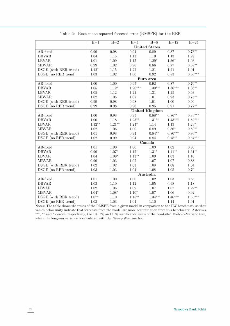
Narodowy Bank Polski28
Table 2: Root mean squared forecast error (RMSFE) for the RER
H=1 H=2 H=4 H=8 H=12 H=24United States
AR-fixed 0.99 0.98 0.94 0.89 0.87 0.73∗∗
DBVAR 1.04 1.15 1.13 1.19 1.13 1.28LBVAR 1.01 1.09 1.15 1.29∗ 1.36∗ 1.03MBVAR 0.99 1.02 0.96 0.86 0.77 0.68∗∗
DSGE (with RER trend) 1.12∗ 1.15 1.22 1.21 1.21 1.01DSGE (no RER trend) 1.03 1.02 1.00 0.92 0.83 0.66∗∗∗
Euro areaAR-fixed 1.00 1.00 0.97 0.92 0.87 0.76∗∗
DBVAR 1.05 1.12∗ 1.20∗∗∗ 1.30∗∗∗ 1.36∗∗∗ 1.36∗∗
LBVAR 1.05 1.12 1.22 1.31 1.25 0.93MBVAR 1.02 1.05 1.07 1.01 0.93 0.75∗∗
DSGE (with RER trend) 0.99 0.98 0.98 1.01 1.00 0.90DSGE (no RER trend) 0.99 0.98 0.96 0.95 0.91 0.77∗∗
United KingdomAR-fixed 1.00 0.98 0.95 0.88∗∗ 0.86∗∗ 0.83∗∗∗
DBVAR 1.06 1.18 1.23∗∗ 1.31∗∗ 1.43∗∗∗ 1.82∗∗∗
LBVAR 1.12∗∗ 1.21∗∗ 1.24∗ 1.14 1.13 1.23∗
MBVAR 1.02 1.06 1.00 0.89 0.86∗ 0.82∗∗
DSGE (with RER trend) 1.01 0.98 0.94 0.84∗∗ 0.80∗∗∗ 0.86∗∗
DSGE (no RER trend) 1.02 0.99 0.94 0.84 0.78∗∗ 0.67∗∗∗
CanadaAR-fixed 1.01 1.00 1.00 1.03 1.02 0.80DBVAR 0.99 1.07∗ 1.15∗ 1.31∗ 1.41∗∗ 1.61∗∗
LBVAR 1.04 1.09∗ 1.13∗∗ 1.09 1.03 1.10MBVAR 0.99 1.03 1.05 1.07 1.07 0.88DSGE (with RER trend) 1.02 1.02 1.03 1.08 1.08 1.04DSGE (no RER trend) 1.03 1.03 1.04 1.08 1.05 0.79
AustraliaAR-fixed 1.01 1.00 1.00 1.02 1.03 0.88DBVAR 1.03 1.10 1.12 1.05 0.98 1.18LBVAR 1.02 1.06 1.09 1.07 1.07 1.22∗∗
MBVAR 1.04∗ 1.08∗ 1.10∗ 1.07 1.06 0.92DSGE (with RER trend) 1.07∗ 1.10 1.18∗∗ 1.34∗∗∗ 1.46∗∗∗ 1.55∗∗∗
DSGE (no RER trend) 1.03 1.03 1.04 1.10 1.14 1.01Notes: The table shows the ratios of the RMSFE from a given model in comparison to the RW benchmark so thatvalues below unity indicate that forecasts from the model are more accurate than from this benchmark. Asterisks∗∗∗, ∗∗ and ∗ denote, respectively, the 1%, 5% and 10% significance levels of the two-tailed Diebold-Mariano test,where the long-run variance is calculated with the Newey-West method.
28
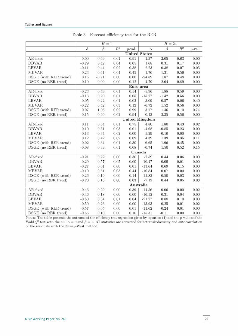
29NBP Working Paper No. 260
Tables and figures
Table 3: Forecast efficiency test for the RER
H = 1 H = 24
α β R2 p-val. α β R2 p-val.United States
AR-fixed 0.00 0.69 0.01 0.91 1.37 2.05 0.63 0.00DBVAR -0.29 0.42 0.04 0.05 1.68 0.31 0.17 0.00LBVAR -0.11 0.44 0.02 0.38 2.23 0.38 0.07 0.05MBVAR -0.23 0.61 0.04 0.45 1.76 1.31 0.56 0.00DSGE (with RER trend) 0.15 -0.21 0.00 0.00 -24.89 1.87 0.48 0.00DSGE (no RER trend) -0.10 0.09 0.00 0.12 -4.79 2.64 0.89 0.00
Euro areaAR-fixed -0.23 0.49 0.01 0.54 -5.96 1.88 0.59 0.00DBVAR -0.13 0.20 0.01 0.05 -15.77 -1.42 0.56 0.00LBVAR -0.05 0.22 0.01 0.02 -3.09 0.57 0.06 0.40MBVAR -0.22 0.42 0.03 0.12 -6.72 1.52 0.56 0.00DSGE (with RER trend) 0.07 1.06 0.02 0.99 3.77 1.46 0.10 0.74DSGE (no RER trend) -0.15 0.99 0.02 0.94 0.43 2.35 0.56 0.00
United KingdomAR-fixed 0.11 0.64 0.01 0.75 4.80 1.80 0.43 0.02DBVAR 0.10 0.31 0.03 0.01 -4.68 -0.85 0.23 0.00LBVAR -0.13 -0.34 0.02 0.00 5.29 -0.16 0.00 0.00MBVAR 0.12 0.42 0.02 0.09 4.39 1.39 0.35 0.11DSGE (with RER trend) -0.02 0.34 0.01 0.30 6.65 1.96 0.45 0.00DSGE (no RER trend) -0.08 0.33 0.01 0.08 -0.74 1.50 0.52 0.15
CanadaAR-fixed -0.21 0.22 0.00 0.30 -7.59 0.44 0.06 0.00DBVAR -0.29 0.57 0.05 0.00 -10.47 -0.09 0.01 0.00LBVAR -0.27 0.01 0.00 0.01 -13.64 0.69 0.15 0.00MBVAR -0.10 0.61 0.03 0.44 -10.84 0.07 0.00 0.00DSGE (with RER trend) -0.26 0.19 0.00 0.14 -11.83 0.50 0.03 0.00DSGE (no RER trend) -0.20 0.15 0.00 0.03 -7.12 0.44 0.05 0.03
AustraliaAR-fixed -0.46 0.29 0.00 0.39 -14.56 0.06 0.00 0.02DBVAR -0.46 0.18 0.00 0.00 -16.52 0.31 0.04 0.00LBVAR -0.50 0.34 0.01 0.04 -21.77 0.88 0.10 0.00MBVAR -0.50 -0.26 0.00 0.00 -13.93 0.25 0.01 0.02DSGE (with RER trend) -0.57 0.05 0.00 0.01 -11.62 -0.24 0.01 0.00DSGE (no RER trend) -0.55 0.10 0.00 0.10 -15.31 -0.11 0.00 0.00
Notes: The table presents the outcome of the efficiency test regression given by equation (1) and the p-values of theWald χ2 test with the null α = 0 and β = 1. All statistics are corrected for heteroskedasticity and autocorrelationof the residuals with the Newey-West method.
29
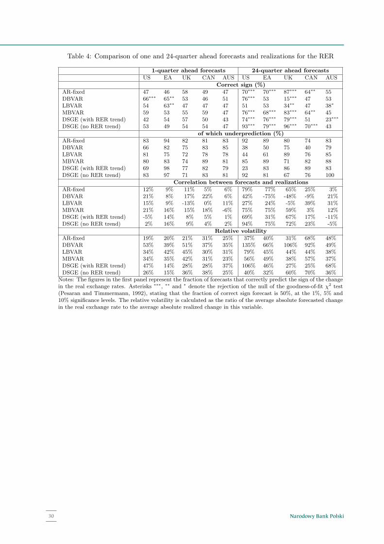
Narodowy Bank Polski30
Table 4: Comparison of one and 24-quarter ahead forecasts and realizations for the RER
1-quarter ahead forecasts 24-quarter ahead forecasts
US EA UK CAN AUS US EA UK CAN AUS
Correct sign (%)
AR-fixed 47 46 58 49 47 70∗∗∗ 70∗∗∗ 87∗∗∗ 64∗∗ 55DBVAR 66∗∗∗ 65∗∗ 53 46 51 76∗∗∗ 53 15∗∗∗ 47 53LBVAR 54 63∗∗ 47 47 47 51 53 34∗∗ 47 38∗
MBVAR 59 53 55 59 47 76∗∗∗ 68∗∗∗ 83∗∗∗ 64∗∗ 45DSGE (with RER trend) 42 54 57 50 43 74∗∗∗ 76∗∗∗ 79∗∗∗ 51 23∗∗∗
DSGE (no RER trend) 53 49 54 54 47 93∗∗∗ 79∗∗∗ 96∗∗∗ 70∗∗∗ 43
of which underprediction (%)
AR-fixed 83 94 82 81 83 92 89 80 74 83DBVAR 66 82 75 83 85 38 50 75 40 79LBVAR 81 75 72 78 78 44 61 89 76 85MBVAR 80 83 74 89 81 85 89 71 82 88DSGE (with RER trend) 69 98 77 82 79 23 83 86 89 83DSGE (no RER trend) 83 97 71 83 81 92 81 67 76 100
Correlation between forecasts and realizations
AR-fixed 12% 9% 11% 5% 6% 79% 77% 65% 25% 3%DBVAR 21% 8% 17% 22% 6% 42% -75% -48% -9% 21%LBVAR 15% 9% -13% 0% 11% 27% 24% -5% 39% 31%MBVAR 21% 16% 15% 18% -6% 75% 75% 59% 3% 12%DSGE (with RER trend) -5% 14% 8% 5% 1% 69% 31% 67% 17% -11%DSGE (no RER trend) 2% 16% 9% 4% 2% 94% 75% 72% 23% -5%
Relative volatility
AR-fixed 19% 20% 21% 31% 25% 37% 40% 31% 68% 48%DBVAR 53% 39% 51% 37% 35% 135% 66% 106% 92% 49%LBVAR 34% 42% 45% 30% 31% 79% 45% 44% 44% 38%MBVAR 34% 35% 42% 31% 23% 56% 49% 38% 57% 37%DSGE (with RER trend) 47% 14% 28% 28% 37% 106% 46% 27% 25% 68%DSGE (no RER trend) 26% 15% 36% 38% 25% 40% 32% 60% 70% 36%
Notes: The figures in the first panel represent the fraction of forecasts that correctly predict the sign of the changein the real exchange rates. Asterisks ∗∗∗, ∗∗ and ∗ denote the rejection of the null of the goodness-of-fit χ2 test(Pesaran and Timmermann, 1992), stating that the fraction of correct sign forecast is 50%, at the 1%, 5% and10% significance levels. The relative volatility is calculated as the ratio of the average absolute forecasted changein the real exchange rate to the average absolute realized change in this variable.
30
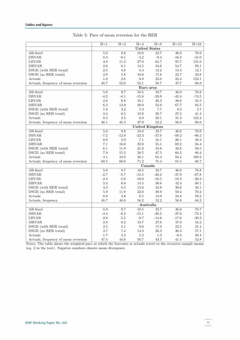
31NBP Working Paper No. 260
Table 5: Pace of mean reversion for the RER
H=1 H=2 H=4 H=8 H=12 H=24
United States
AR-fixed 5.0 9.8 18.6 33.7 46.0 70.8DBVAR 0.4 -0.1 -3.2 -9.4 -16.3 -41.0LBVAR 4.8 11.2 27.0 62.7 95.7 131.6MBVAR 2.6 6.1 14.5 34.6 54.7 93.1DSGE (with RER trend) 2.5 4.8 8.4 12.2 13.4 12.1DSGE (no RER trend) 2.9 5.8 10.8 17.8 22.7 33.8Actuals 1.0 3.8 8.8 23.0 22.4 123.1Actuals, frequency of mean reversion 48.7 52.0 52.1 50.7 47.7 69.8
Euro area
AR-fixed 5.0 9.7 18.5 33.7 46.0 70.8DBVAR -4.2 -8.1 -15.8 -29.9 -42.4 -74.5LBVAR 2.8 6.8 16.1 30.3 38.6 45.5MBVAR 6.3 13.9 29.0 52.9 67.7 84.5DSGE (with RER trend) 1.8 3.2 5.3 7.7 8.3 5.7DSGE (no RER trend) 3.4 6.5 12.0 20.7 27.4 41.4Actuals 0.5 2.5 6.9 20.1 31.3 122.2Actuals, frequency of mean reversion 46.1 45.3 47.9 52.2 56.9 69.8
United Kingdom
AR-fixed 5.0 9.8 18.6 33.7 46.0 70.8DBVAR -7.2 -12.9 -22.3 -37.0 -50.2 -86.2LBVAR 0.9 2.9 7.1 16.1 26.1 39.3MBVAR 7.1 16.0 32.0 55.1 69.2 84.4DSGE (with RER trend) 6.1 11.9 21.6 34.8 42.6 50.5DSGE (no RER trend) 7.9 15.5 28.5 47.5 60.3 80.4Actuals 4.1 10.9 26.1 65.4 94.4 169.2Actuals, frequency of mean reversion 60.5 60.0 71.2 75.4 81.5 88.7
Canada
AR-fixed 5.0 9.7 18.5 33.7 46.0 70.8DBVAR -2.7 -5.7 -12.5 -26.2 -37.9 -67.8LBVAR -2.4 -5.0 -10.0 -16.5 -18.3 -30.3MBVAR 2.4 6.0 14.5 30.6 42.4 60.1DSGE (with RER trend) 4.3 8.5 15.6 24.8 30.0 34.1DSGE (no RER trend) 5.9 11.9 22.6 38.9 50.4 70.2Actuals 0.8 3.8 8.5 14.0 24.4 59.2Actuals, frequency 48.7 48.0 56.2 52.2 50.8 64.2
Australia
AR-fixed 5.0 9.7 18.5 33.7 46.0 70.7DBVAR -4.4 -8.2 -15.1 -26.2 -37.0 -72.4LBVAR -2.8 -5.5 -9.7 -14.6 -17.6 -30.3MBVAR 2.8 6.2 13.7 27.0 37.0 54.2DSGE (with RER trend) 2.5 5.1 9.6 17.0 22.5 31.4DSGE (no RER trend) 3.7 7.4 14.3 26.3 36.3 57.1Actuals 1.7 4.2 5.2 1.3 -0.4 20.4Actuals, frequency of mean reversion 47.4 44.0 50.7 43.5 41.5 52.8
Notes: The table shows the weighted pace at which the forecasts or actuals revert to the recursive sample means(eq. 2 in the text). Negative numbers denote mean divergence.
31
Tables and figures
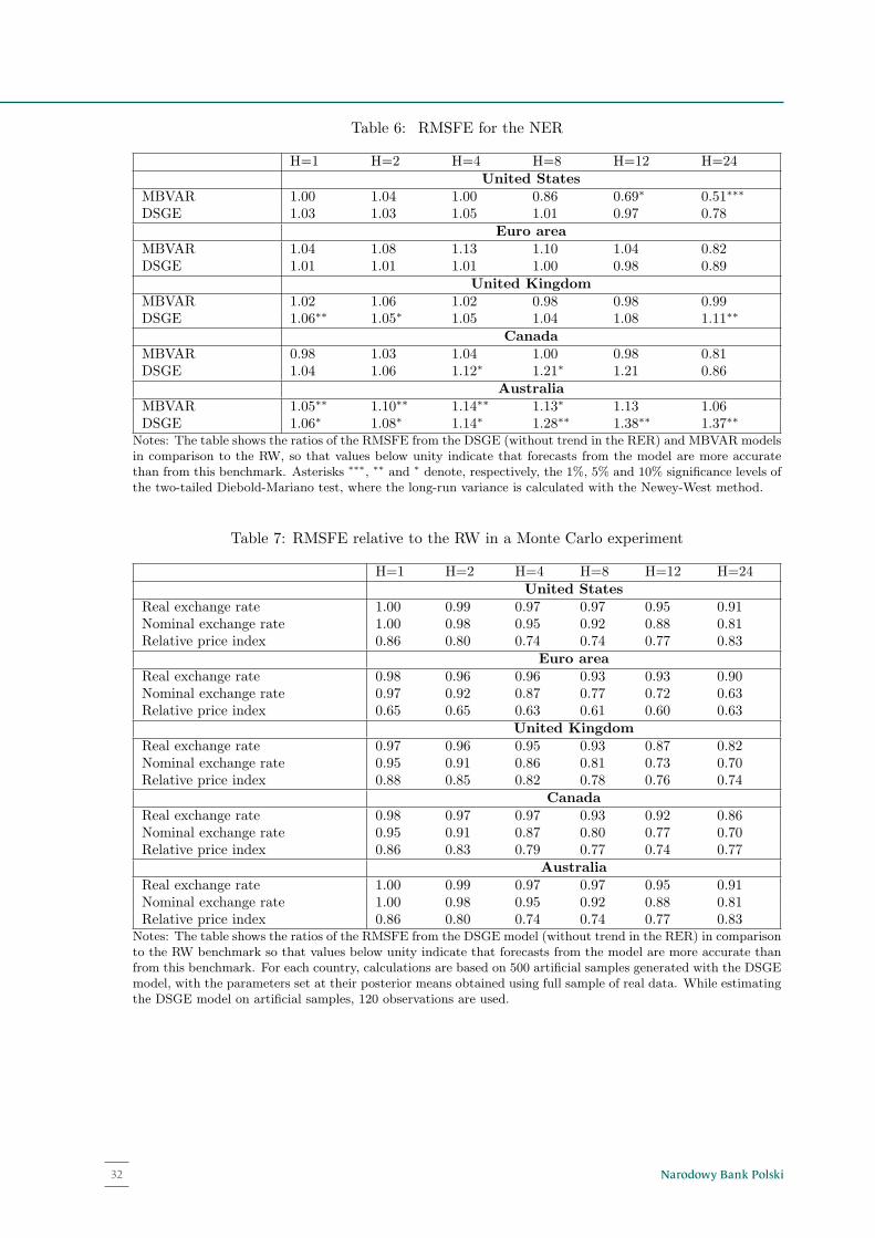
Narodowy Bank Polski32
Table 6: RMSFE for the NER
H=1 H=2 H=4 H=8 H=12 H=24United States
MBVAR 1.00 1.04 1.00 0.86 0.69∗ 0.51∗∗∗
DSGE 1.03 1.03 1.05 1.01 0.97 0.78Euro area
MBVAR 1.04 1.08 1.13 1.10 1.04 0.82DSGE 1.01 1.01 1.01 1.00 0.98 0.89
United KingdomMBVAR 1.02 1.06 1.02 0.98 0.98 0.99DSGE 1.06∗∗ 1.05∗ 1.05 1.04 1.08 1.11∗∗
CanadaMBVAR 0.98 1.03 1.04 1.00 0.98 0.81DSGE 1.04 1.06 1.12∗ 1.21∗ 1.21 0.86
AustraliaMBVAR 1.05∗∗ 1.10∗∗ 1.14∗∗ 1.13∗ 1.13 1.06DSGE 1.06∗ 1.08∗ 1.14∗ 1.28∗∗ 1.38∗∗ 1.37∗∗
Notes: The table shows the ratios of the RMSFE from the DSGE (without trend in the RER) and MBVAR modelsin comparison to the RW, so that values below unity indicate that forecasts from the model are more accuratethan from this benchmark. Asterisks ∗∗∗, ∗∗ and ∗ denote, respectively, the 1%, 5% and 10% significance levels ofthe two-tailed Diebold-Mariano test, where the long-run variance is calculated with the Newey-West method.
Table 7: RMSFE relative to the RW in a Monte Carlo experiment
H=1 H=2 H=4 H=8 H=12 H=24United States
Real exchange rate 1.00 0.99 0.97 0.97 0.95 0.91Nominal exchange rate 1.00 0.98 0.95 0.92 0.88 0.81Relative price index 0.86 0.80 0.74 0.74 0.77 0.83
Euro areaReal exchange rate 0.98 0.96 0.96 0.93 0.93 0.90Nominal exchange rate 0.97 0.92 0.87 0.77 0.72 0.63Relative price index 0.65 0.65 0.63 0.61 0.60 0.63
United KingdomReal exchange rate 0.97 0.96 0.95 0.93 0.87 0.82Nominal exchange rate 0.95 0.91 0.86 0.81 0.73 0.70Relative price index 0.88 0.85 0.82 0.78 0.76 0.74
CanadaReal exchange rate 0.98 0.97 0.97 0.93 0.92 0.86Nominal exchange rate 0.95 0.91 0.87 0.80 0.77 0.70Relative price index 0.86 0.83 0.79 0.77 0.74 0.77
AustraliaReal exchange rate 1.00 0.99 0.97 0.97 0.95 0.91Nominal exchange rate 1.00 0.98 0.95 0.92 0.88 0.81Relative price index 0.86 0.80 0.74 0.74 0.77 0.83
Notes: The table shows the ratios of the RMSFE from the DSGE model (without trend in the RER) in comparisonto the RW benchmark so that values below unity indicate that forecasts from the model are more accurate thanfrom this benchmark. For each country, calculations are based on 500 artificial samples generated with the DSGEmodel, with the parameters set at their posterior means obtained using full sample of real data. While estimatingthe DSGE model on artificial samples, 120 observations are used.
32
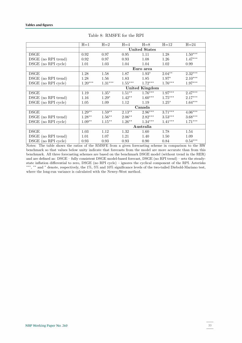
33NBP Working Paper No. 260
Table 8: RMSFE for the RPI
H=1 H=2 H=4 H=8 H=12 H=24United States
DSGE 0.92 0.97 0.95 1.11 1.28 1.50∗∗∗
DSGE (no RPI trend) 0.92 0.97 0.93 1.08 1.26 1.47∗∗∗
DSGE (no RPI cycle) 1.01 1.03 1.04 1.04 1.02 0.99Euro area
DSGE 1.28 1.58 1.87 1.93∗ 2.04∗∗ 2.32∗∗∗
DSGE (no RPI trend) 1.28 1.56 1.83 1.85 1.97∗ 2.10∗∗∗
DSGE (no RPI cycle) 1.20∗∗∗ 1.31∗∗∗ 1.55∗∗∗ 1.72∗∗∗ 1.76∗∗∗ 1.97∗∗∗
United KingdomDSGE 1.19 1.35∗ 1.51∗∗ 1.76∗∗∗ 1.97∗∗∗ 2.47∗∗∗
DSGE (no RPI trend) 1.16 1.29∗ 1.42∗∗ 1.60∗∗∗ 1.75∗∗∗ 2.17∗∗∗
DSGE (no RPI cycle) 1.05 1.09 1.12 1.19 1.25∗ 1.64∗∗∗
CanadaDSGE 1.29∗∗ 1.59∗∗ 2.13∗∗ 2.96∗∗∗ 3.71∗∗∗ 4.06∗∗∗
DSGE (no RPI trend) 1.28∗∗ 1.56∗∗ 2.06∗∗ 2.82∗∗∗ 3.53∗∗∗ 3.68∗∗∗
DSGE (no RPI cycle) 1.09∗∗ 1.15∗∗ 1.26∗∗ 1.34∗∗∗ 1.41∗∗∗ 1.71∗∗∗
AustraliaDSGE 1.03 1.12 1.32 1.60 1.78 1.54DSGE (no RPI trend) 1.01 1.07 1.21 1.40 1.50 1.09DSGE (no RPI cycle) 0.93 0.93 0.93 0.90 0.84 0.54∗∗∗
Notes: The table shows the ratios of the RMSFE from a given forecasting scheme in comparison to the RWbenchmark so that values below unity indicate that forecasts from the model are more accurate than from thisbenchmark. All three forecasting schemes are based on the benchmark DSGE model (without trend in the RER)and are defined as: DSGE – fully consistent DSGE model-based forecast, DSGE (no RPI trend) – sets the steady-state inflation differential to zero, DSGE (no RPI cycle) – ignores the cyclical component of the RPI. Asterisks∗∗∗, ∗∗ and ∗ denote, respectively, the 1%, 5% and 10% significance levels of the two-tailed Diebold-Mariano test,where the long-run variance is calculated with the Newey-West method.
33
Tables and figures
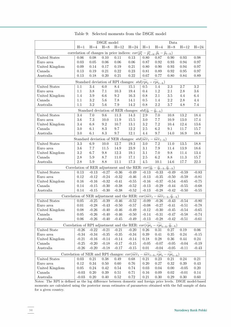
Narodowy Bank Polski34
Table 9: Selected moments from the DSGE model
DSGE model DataH=1 H=4 H=8 H=12 H=24 H=1 H=4 H=8 H=12 H=24
correlation of changes in price indices: cor(p∗t − p∗t−h, pt − pt−h)United States 0.06 0.08 0.10 0.11 0.13 0.80 0.87 0.90 0.93 0.98Euro area 0.03 0.05 0.06 0.06 0.06 0.87 0.92 0.93 0.94 0.97United Kingdom 0.09 0.14 0.17 0.19 0.21 0.80 0.90 0.93 0.94 0.97Canada 0.13 0.19 0.21 0.22 0.23 0.81 0.89 0.92 0.95 0.97Australia 0.13 0.18 0.20 0.21 0.22 0.67 0.77 0.80 0.84 0.89
Standard deviation of RPI changes: std(rpit − rpit−h)United States 1.1 3.4 6.0 8.4 15.1 0.5 1.4 2.3 2.7 3.2Euro area 1.1 3.8 7.1 10.3 19.4 0.4 1.2 2.1 2.8 3.6United Kingdom 1.4 3.9 6.6 9.2 16.3 0.8 2.1 3.5 4.4 6.4Canada 1.1 3.2 5.6 7.8 14.1 0.5 1.4 2.2 2.8 4.4Australia 1.1 3.2 5.6 7.9 14.2 0.8 2.2 3.7 4.8 7.4
Standard deviation of RER changes: std(qt − qt−h)United States 3.4 7.0 9.6 11.3 14.3 2.9 7.0 10.8 13.2 18.4Euro area 3.6 7.3 10.0 11.9 15.5 3.0 7.7 10.9 13.0 17.4United Kingdom 3.4 6.8 9.2 10.7 13.1 3.2 7.2 10.4 12.4 13.6Canada 3.0 6.1 8.3 9.7 12.2 2.5 6.2 9.1 11.7 15.7Australia 3.0 6.1 8.3 9.7 12.1 4.4 9.7 14.0 16.9 18.8
Standard deviation of NER changes: std(nert − nert−h)United States 3.3 6.9 10.0 12.7 19.3 3.0 7.2 11.0 13.5 18.8Euro area 3.6 7.7 11.5 14.9 23.9 3.1 7.9 11.4 13.9 18.6United Kingdom 3.2 6.7 9.8 12.3 19.1 3.1 7.0 9.8 11.4 13.4Canada 2.8 5.9 8.7 11.0 17.1 2.5 6.2 8.8 11.3 15.7Australia 2.8 5.9 8.8 11.1 17.3 4.5 10.1 14.6 17.7 22.3
Correlation of RER adjustment and the RER: cor(qt − qt−h, qt−h)United States 0.13 -0.13 -0.27 -0.36 -0.49 -0.13 -0.33 -0.49 -0.59 -0.83Euro area 0.12 -0.12 -0.24 -0.32 -0.46 -0.13 -0.35 -0.50 -0.59 -0.81United Kingdom 0.16 -0.16 -0.32 -0.41 -0.55 -0.16 -0.37 -0.54 -0.65 -0.75Canada 0.14 -0.15 -0.30 -0.38 -0.52 -0.13 -0.29 -0.44 -0.55 -0.68Australia 0.14 -0.15 -0.30 -0.38 -0.52 -0.13 -0.28 -0.42 -0.50 -0.55
Correlation of NER adjustment and the RER: cor(nert − nert−h, qt−h)United States 0.05 -0.25 -0.39 -0.46 -0.52 -0.09 -0.26 -0.43 -0.54 -0.80Euro area 0.01 -0.28 -0.43 -0.50 -0.57 -0.08 -0.27 -0.41 -0.51 -0.78United Kingdom 0.08 -0.26 -0.40 -0.46 -0.49 -0.12 -0.30 -0.45 -0.54 -0.65Canada 0.05 -0.26 -0.40 -0.46 -0.50 -0.14 -0.31 -0.47 -0.58 -0.74Australia 0.06 -0.26 -0.40 -0.45 -0.49 -0.13 -0.28 -0.42 -0.51 -0.61
Correlation of RPI adjustment and the RER: cor(rpit − rpit−h, qt−h)United State -0.26 -0.22 -0.21 -0.21 -0.20 0.26 0.31 0.27 0.19 0.06Euro area -0.34 -0.34 -0.35 -0.35 -0.34 0.39 0.41 0.35 0.24 -0.15United Kingdom -0.21 -0.16 -0.14 -0.14 -0.14 0.18 0.28 0.36 0.44 0.24Canada -0.25 -0.20 -0.18 -0.17 -0.15 -0.05 -0.07 -0.05 -0.04 -0.19Australia -0.26 -0.20 -0.18 -0.17 -0.15 0.01 -0.04 -0.05 -0.11 -0.43
Correlation of NER and RPI changes: cor(nert − nert−h, rpit − rpit−h)United States 0.03 0.21 0.38 0.49 0.68 0.21 0.23 0.21 0.24 0.21Euro area 0.12 0.34 0.50 0.60 0.76 0.20 0.27 0.32 0.39 0.43United Kingdom 0.05 0.24 0.42 0.54 0.74 0.03 0.04 0.00 -0.05 0.20Canada -0.03 0.20 0.39 0.51 0.71 0.16 0.09 0.02 -0.01 0.14Australia -0.03 0.20 0.40 0.52 0.72 0.21 0.30 0.29 0.30 0.60
Notes: The RPI is defined as the log difference between domestic and foreign price levels. DSGE model-basedmoments are calculated using the posterior mean estimates of parameters obtained with the full sample of datafor a given country.
34
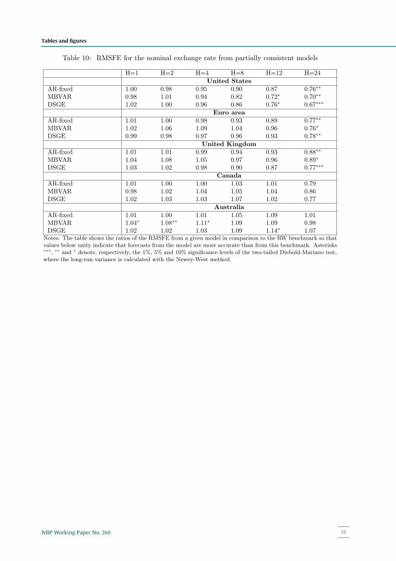
35NBP Working Paper No. 260
Table 10: RMSFE for the nominal exchange rate from partially consistent models
H=1 H=2 H=4 H=8 H=12 H=24United States
AR-fixed 1.00 0.98 0.95 0.90 0.87 0.76∗∗
MBVAR 0.98 1.01 0.94 0.82 0.72∗ 0.70∗∗
DSGE 1.02 1.00 0.96 0.86 0.76∗ 0.67∗∗∗
Euro areaAR-fixed 1.01 1.00 0.98 0.93 0.89 0.77∗∗
MBVAR 1.02 1.06 1.09 1.04 0.96 0.76∗
DSGE 0.99 0.98 0.97 0.96 0.93 0.78∗∗
United KingdomAR-fixed 1.01 1.01 0.99 0.94 0.93 0.88∗∗
MBVAR 1.04 1.08 1.05 0.97 0.96 0.89∗
DSGE 1.03 1.02 0.98 0.90 0.87 0.77∗∗∗
CanadaAR-fixed 1.01 1.00 1.00 1.03 1.01 0.79MBVAR 0.98 1.02 1.04 1.05 1.04 0.86DSGE 1.02 1.03 1.03 1.07 1.02 0.77
AustraliaAR-fixed 1.01 1.00 1.01 1.05 1.09 1.01MBVAR 1.04∗ 1.08∗∗ 1.11∗ 1.09 1.09 0.98DSGE 1.02 1.02 1.03 1.09 1.14∗ 1.07
Notes: The table shows the ratios of the RMSFE from a given model in comparison to the RW benchmark so thatvalues below unity indicate that forecasts from the model are more accurate than from this benchmark. Asterisks∗∗∗, ∗∗ and ∗ denote, respectively, the 1%, 5% and 10% significance levels of the two-tailed Diebold-Mariano test,where the long-run variance is calculated with the Newey-West method.
35
Tables and figures
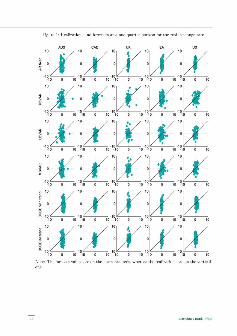
Narodowy Bank Polski36
Figure 2: Realizations and forecasts at a six-year horizon for the real exchange rate
-50 0 50-50
0
50AUS
AR fi
xed
-50 0 50-50
0
50CAD
-50 0 50-50
0
50UK
-50 0 50-50
0
50EA
-50 0 50-50
0
50US
-50 0 50-50
0
50
DBV
AR
-50 0 50-50
0
50
-50 0 50-50
0
50
-50 0 50-50
0
50
-50 0 50-50
0
50
-50 0 50-50
0
50
LBVA
R
-50 0 50-50
0
50
-50 0 50-50
0
50
-50 0 50-50
0
50
-50 0 50-50
0
50
-50 0 50-50
0
50
MBV
AR
-50 0 50-50
0
50
-50 0 50-50
0
50
-50 0 50-50
0
50
-50 0 50-50
0
50
-50 0 50-50
0
50
DSG
E w
ith tr
end
-50 0 50-50
0
50
-50 0 50-50
0
50
-50 0 50-50
0
50
-50 0 50-50
0
50
-50 0 50-50
0
50
DSG
E no
tren
d
-50 0 50-50
0
50
-50 0 50-50
0
50
-50 0 50-50
0
50
-50 0 50-50
0
50
Note: The forecast values are on the horizontal axis, whereas the realizations are on the verticalone.
37
Figure 1: Realizations and forecasts at a one-quarter horizon for the real exchange rate
Note: The forecast values are on the horizontal axis, whereas the realizations are on the verticalone.
36
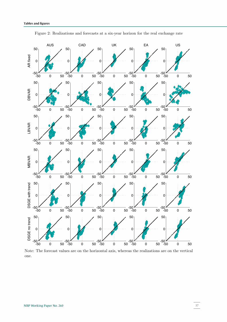
37NBP Working Paper No. 260
Figure 2: Realizations and forecasts at a six-year horizon for the real exchange rate
-50 0 50-50
0
50AUS
AR fi
xed
-50 0 50-50
0
50CAD
-50 0 50-50
0
50UK
-50 0 50-50
0
50EA
-50 0 50-50
0
50US
-50 0 50-50
0
50
DBV
AR
-50 0 50-50
0
50
-50 0 50-50
0
50
-50 0 50-50
0
50
-50 0 50-50
0
50
-50 0 50-50
0
50
LBVA
R
-50 0 50-50
0
50
-50 0 50-50
0
50
-50 0 50-50
0
50
-50 0 50-50
0
50
-50 0 50-50
0
50
MBV
AR
-50 0 50-50
0
50
-50 0 50-50
0
50
-50 0 50-50
0
50
-50 0 50-50
0
50
-50 0 50-50
0
50
DSG
E w
ith tr
end
-50 0 50-50
0
50
-50 0 50-50
0
50
-50 0 50-50
0
50
-50 0 50-50
0
50
-50 0 50-50
0
50
DSG
E no
tren
d
-50 0 50-50
0
50
-50 0 50-50
0
50
-50 0 50-50
0
50
-50 0 50-50
0
50
Note: The forecast values are on the horizontal axis, whereas the realizations are on the verticalone.
37
Tables and figures
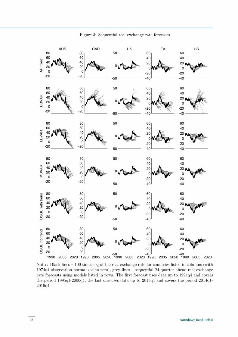
Narodowy Bank Polski38
Figure 3: Sequential real exchange rate forecasts
-200
20406080
AUS
AR fi
xed
-200
20406080
CAD
-50
0
50UK
-40-20
0204060
EA
-40-20
0204060
US
-200
20406080
DBV
AR
-200
20406080
-50
0
50
-40-20
0204060
-40-20
0204060
-200
20406080
LBVA
R
-200
20406080
-50
0
50
-40-20
0204060
-40-20
0204060
-200
20406080
MBV
AR
-200
20406080
-50
0
50
-40-20
0204060
-40-20
0204060
-200
20406080
DSG
E w
ith tr
end
-200
20406080
-50
0
50
-40-20
0204060
-40-20
0204060
1990 2005 2020-20
020406080
DSG
E no
tren
d
1990 2005 2020-20
020406080
1990 2005 2020-50
0
50
1990 2005 2020-40-20
0204060
1990 2005 2020-40-20
0204060
Notes: Black lines – 100 times log of the real exchange rate for countries listed in columns (with1974q4 observation normalized to zero), grey lines – sequential 24-quarter ahead real exchangerate forecasts using models listed in rows. The first forecast uses data up to 1994q4 and coversthe period 1995q1-2000q4, the last one uses data up to 2013q4 and covers the period 2014q1-2019q4.
38
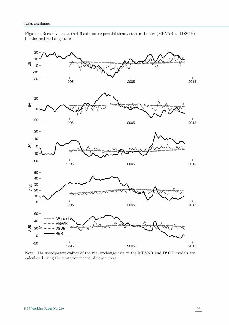
39NBP Working Paper No. 260
Figure 4: Recursive mean (AR-fixed) and sequential steady state estimates (MBVAR and DSGE)for the real exchange rate
1995 2005 2015-20
-10
0
10
20
US
1995 2005 2015-20
0
20
EA
1995 2005 2015-20
-10
0
10
20
UK
1995 2005 20150
1020304050
CAD
1995 2005 2015-20
0
20
40
60
AUS
AR fixedMBVARDSGERER
Note: The steady-state-values of the real exchange rate in the MBVAR and DSGE models arecalculated using the posterior means of parameters.
39
Tables and figures
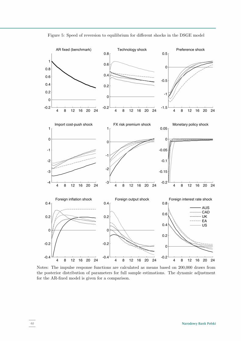
Narodowy Bank Polski40
Figure 5: Speed of reversion to equilibrium for different shocks in the DSGE model
4 8 12 16 20 24-0.2
0
0.2
0.4
0.6
0.8Technology shock
4 8 12 16 20 24-1.5
-1
-0.5
0
0.5Preference shock
4 8 12 16 20 24-4
-3
-2
-1
0
1Import cost-push shock
4 8 12 16 20 24-3
-2
-1
0
1FX risk premium shock
4 8 12 16 20 24-0.2
-0.15
-0.1
-0.05
0
0.05Monetary policy shock
4 8 12 16 20 24-0.4
-0.2
0
0.2
0.4Foreign inflation shock
4 8 12 16 20 24-0.4
-0.2
0
0.2
0.4Foreign output shock
4 8 12 16 20 24-0.2
0
0.2
0.4
0.6
0.8Foreign interest rate shock
AUSCADUKEAUS
4 8 12 16 20 24-0.2
0
0.2
0.4
0.6
0.8
1
AR fixed (benchmark)
Notes: The impulse response functions are calculated as means based on 200,000 draws fromthe posterior distribution of parameters for full sample estimations. The dynamic adjustmentfor the AR-fixed model is given for a comparison.
40
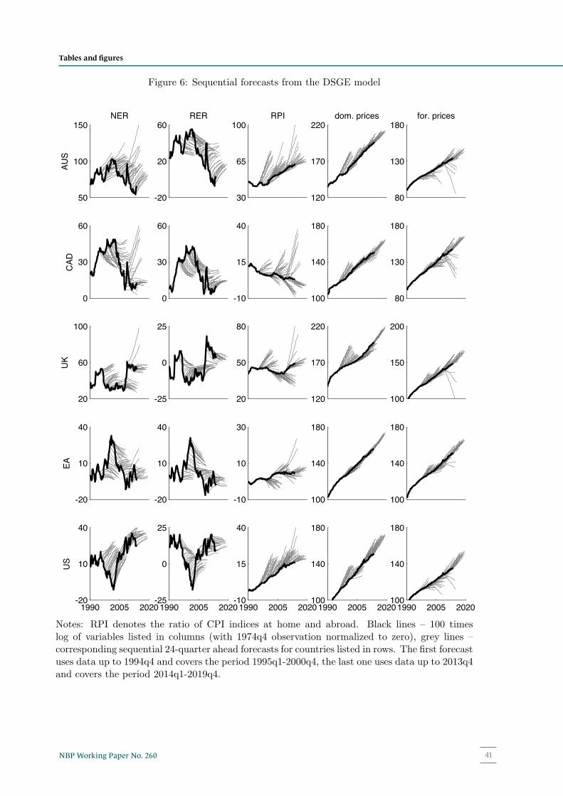
41NBP Working Paper No. 260
Figure 6: Sequential forecasts from the DSGE model
50
100
150NER
AUS
-20
20
60RER
30
65
100RPI
120
170
220dom. prices
80
130
180for. prices
0
30
60
CAD
0
30
60
-10
15
40
100
140
180
80
130
180
20
60
100
UK
-25
0
25
20
50
80
120
170
220
100
150
200
-20
10
40
EA
-20
10
40
-10
10
30
100
140
180
100
140
180
1990 2005 2020-20
10
40
US
1990 2005 2020-25
0
25
1990 2005 2020-10
15
40
1990 2005 2020100
140
180
1990 2005 2020100
140
180
Notes: RPI denotes the ratio of CPI indices at home and abroad. Black lines – 100 timeslog of variables listed in columns (with 1974q4 observation normalized to zero), grey lines –corresponding sequential 24-quarter ahead forecasts for countries listed in rows. The first forecastuses data up to 1994q4 and covers the period 1995q1-2000q4, the last one uses data up to 2013q4and covers the period 2014q1-2019q4.
41
Tables and figures
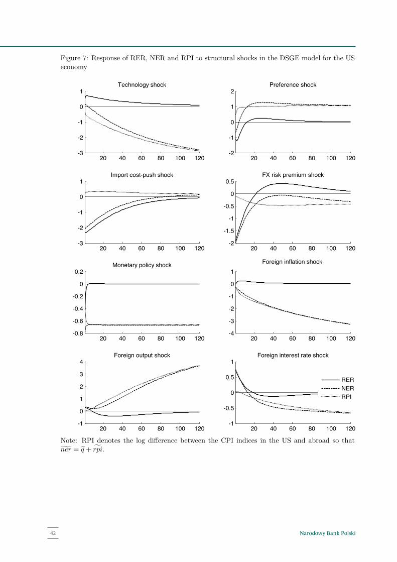
Narodowy Bank Polski42
Figure 7: Response of RER, NER and RPI to structural shocks in the DSGE model for the USeconomy
20 40 60 80 100 120-3
-2
-1
0
1Technology shock
20 40 60 80 100 120-2
-1
0
1
2Preference shock
20 40 60 80 100 120-3
-2
-1
0
1Import cost-push shock
20 40 60 80 100 120-2
-1.5
-1
-0.5
0
0.5FX risk premium shock
20 40 60 80 100 120-0.8
-0.6
-0.4
-0.2
0
0.2Monetary policy shock
20 40 60 80 100 120-4
-3
-2
-1
0
1Foreign inflation shock
20 40 60 80 100 120-1
0
1
2
3
4Foreign output shock
20 40 60 80 100 120-1
-0.5
0
0.5
1Foreign interest rate shock
RERNERRPI
Note: RPI denotes the log difference between the CPI indices in the US and abroad so thatner = q + rpi.
42
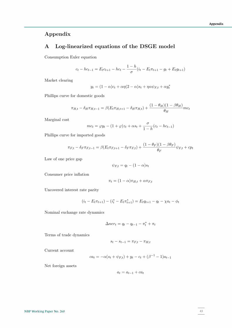
43NBP Working Paper No. 260
Appendix
A Log-linearized equations of the DSGE model
Consumption Euler equation
ct − hct−1 = Etct+1 − hct −1− h
σ(it − Etπt+1 − gt + Etgt+1)
Market clearing
yt = (1− α)ct + αη(2− α)st + ηαψF,t + αy∗t
Phillips curve for domestic goods
πH,t − δHπH,t−1 = β(EtπH,t+1 − δHπH,t) +(1− θH)(1− βθH)
θHmct
Marginal cost
mct = ϕyt − (1 + ϕ)zt + αst +σ
1− h(ct − hct−1)
Phillips curve for imported goods
πF,t − δFπF,t−1 = β(EtπF,t+1 − δFπF,t) +(1− θF )(1− βθF )
θFψF,t + cpt
Law of one price gap
ψF,t = qt − (1− α)st
Consumer price inflation
πt = (1− α)πH,t + απF,t
Uncovered interest rate parity
(it − Etπt+1)− (i∗t − Etπ∗t+1) = Etqt+1 − qt − χat − φt
Nominal exchange rate dynamics
∆nert = qt − qt−1 − π∗t + πt
Terms of trade dynamics
st − st−1 = πF,t − πH,t
Current account
cat = −α(st + ψF,t) + yt − ct + (β−1 − 1)at−1
Net foreign assets
at = at−1 + cat
43
Appendix
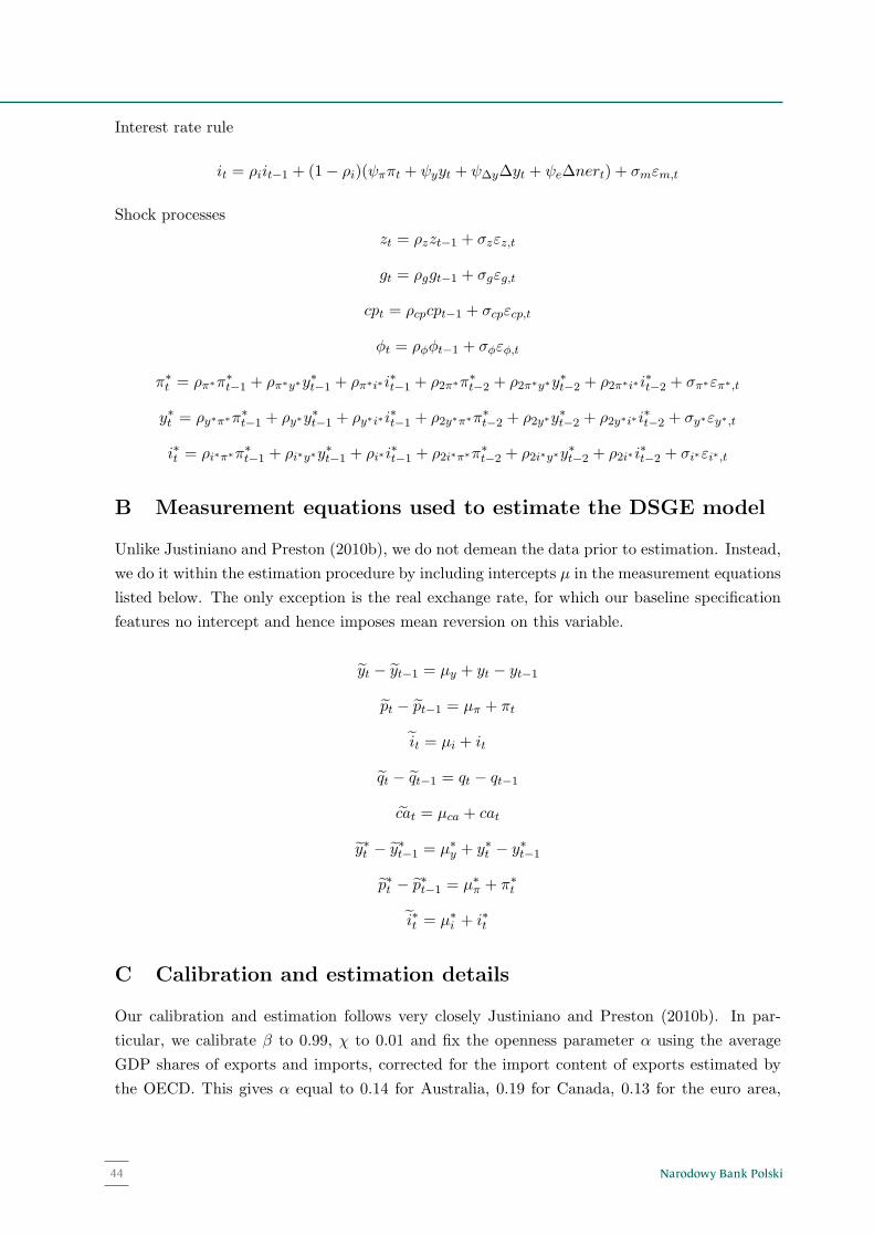
Narodowy Bank Polski44
Interest rate rule
it = ρiit−1 + (1− ρi)(ψππt + ψyyt + ψ∆y∆yt + ψe∆nert) + σmεm,t
Shock processes
zt = ρzzt−1 + σzεz,t
gt = ρggt−1 + σgεg,t
cpt = ρcpcpt−1 + σcpεcp,t
φt = ρφφt−1 + σφεφ,t
π∗t = ρπ∗π∗
t−1 + ρπ∗y∗y∗t−1 + ρπ∗i∗i
∗t−1 + ρ2π∗π∗
t−2 + ρ2π∗y∗y∗t−2 + ρ2π∗i∗i
∗t−2 + σπ∗επ∗,t
y∗t = ρy∗π∗π∗t−1 + ρy∗y
∗t−1 + ρy∗i∗i
∗t−1 + ρ2y∗π∗π∗
t−2 + ρ2y∗y∗t−2 + ρ2y∗i∗i
∗t−2 + σy∗εy∗,t
i∗t = ρi∗π∗π∗t−1 + ρi∗y∗y
∗t−1 + ρi∗i
∗t−1 + ρ2i∗π∗π∗
t−2 + ρ2i∗y∗y∗t−2 + ρ2i∗i
∗t−2 + σi∗εi∗,t
B Measurement equations used to estimate the DSGE model
Unlike Justiniano and Preston (2010b), we do not demean the data prior to estimation. Instead,
we do it within the estimation procedure by including intercepts µ in the measurement equations
listed below. The only exception is the real exchange rate, for which our baseline specification
features no intercept and hence imposes mean reversion on this variable.
yt − yt−1 = µy + yt − yt−1
pt − pt−1 = µπ + πt
it = µi + it
qt − qt−1 = qt − qt−1
cat = µca + cat
y∗t − y∗t−1 = µ∗y + y∗t − y∗t−1
p∗t − p∗t−1 = µ∗π + π∗
t
i∗t = µ∗i + i∗t
C Calibration and estimation details
Our calibration and estimation follows very closely Justiniano and Preston (2010b). In par-
ticular, we calibrate β to 0.99, χ to 0.01 and fix the openness parameter α using the average
GDP shares of exports and imports, corrected for the import content of exports estimated by
the OECD. This gives α equal to 0.14 for Australia, 0.19 for Canada, 0.13 for the euro area,
44

45NBP Working Paper No. 260
Appendix
0.19 for the United Kingdom and 0.09 for the United States. The remaining parameters are
estimated using Bayesian methods. The prior distributions for the intercepts in the measure-
ment equations are assumed to be uniform and hence uninformative. The prior assumptions for
the remaining parameters are identical to those used by Justiniano and Preston (2010b). The
posterior distributions are approximated with 200,000 draws obtained from four Markov Monte
Carlo chains generated with the Metropolis-Hastings algorithm after burning in the initial 50,000
draws. All these calculations were done using Dynare, version 4.4.3. Detailed estimation results
are available from the authors upon request.
45
Interest rate rule
it = ρiit−1 + (1− ρi)(ψππt + ψyyt + ψ∆y∆yt + ψe∆nert) + σmεm,t
Shock processes
zt = ρzzt−1 + σzεz,t
gt = ρggt−1 + σgεg,t
cpt = ρcpcpt−1 + σcpεcp,t
φt = ρφφt−1 + σφεφ,t
π∗t = ρπ∗π∗
t−1 + ρπ∗y∗y∗t−1 + ρπ∗i∗i
∗t−1 + ρ2π∗π∗
t−2 + ρ2π∗y∗y∗t−2 + ρ2π∗i∗i
∗t−2 + σπ∗επ∗,t
y∗t = ρy∗π∗π∗t−1 + ρy∗y
∗t−1 + ρy∗i∗i
∗t−1 + ρ2y∗π∗π∗
t−2 + ρ2y∗y∗t−2 + ρ2y∗i∗i
∗t−2 + σy∗εy∗,t
i∗t = ρi∗π∗π∗t−1 + ρi∗y∗y
∗t−1 + ρi∗i
∗t−1 + ρ2i∗π∗π∗
t−2 + ρ2i∗y∗y∗t−2 + ρ2i∗i
∗t−2 + σi∗εi∗,t
B Measurement equations used to estimate the DSGE model
Unlike Justiniano and Preston (2010b), we do not demean the data prior to estimation. Instead,
we do it within the estimation procedure by including intercepts µ in the measurement equations
listed below. The only exception is the real exchange rate, for which our baseline specification
features no intercept and hence imposes mean reversion on this variable.
yt − yt−1 = µy + yt − yt−1
pt − pt−1 = µπ + πt
it = µi + it
qt − qt−1 = qt − qt−1
cat = µca + cat
y∗t − y∗t−1 = µ∗y + y∗t − y∗t−1
p∗t − p∗t−1 = µ∗π + π∗
t
i∗t = µ∗i + i∗t
C Calibration and estimation details
Our calibration and estimation follows very closely Justiniano and Preston (2010b). In par-
ticular, we calibrate β to 0.99, χ to 0.01 and fix the openness parameter α using the average
GDP shares of exports and imports, corrected for the import content of exports estimated by
the OECD. This gives α equal to 0.14 for Australia, 0.19 for Canada, 0.13 for the euro area,
44

www.nbp.pl