Distributed Graph Simulation: Impossibility and Possibility

Wenfei Fan1,2 Xin Wang4 Yinghui Wu1,3 Dong Deng5

1University of Edinburgh 2RCBD and SKLSDE Lab, Beihang University 3Washington StateUniversity 4Southwest Jiaotong University 5Tsinghua University

{wenfei@inf, x.wang-36@sms}.ed.ac.uk ywu@eecs.wsu.edu dd11@mails.tsinghua.edu.cn

ABSTRACTThis paper studies fundamental problems for distributedgraph simulation. Given a pattern query Q and a graphG that is fragmented and distributed, a graph simulationalgorithm A is to compute the matches Q(G) of Q in G. Wesay that A is parallel scalable in (a) response time if its paral-lel computational cost is determined by the largest fragmentFm of G and the size |Q| of query Q, and (b) data shipmentif its total amount of data shipped is determined by |Q|and the number of fragments of G, independent of the sizeof graph G. (1) We prove an impossibility theorem: thereexists no distributed graph simulation algorithm that is par-allel scalable in either response time or data shipment. (2)However, we show that distributed graph simulation is par-tition bounded, i.e., its response time depends only on |Q|,|Fm| and the number |Vf | of nodes in G with edges acrossdifferent fragments; and its data shipment depends on |Q|and the number |Ef | of crossing edges only. We provide thefirst algorithms with these performance guarantees. (3) Wealso identify special cases of patterns and graphs when par-allel scalability is possible. (4) We experimentally verify thescalability and efficiency of our algorithms.

1. INTRODUCTIONGraph pattern matching is widely used to search and an-

alyze, e.g., social graphs, biological data and transportationnetworks. Given a graph pattern Q and a data graph G, it isto compute Q(G), the set of all matches of Q in G. In thereal world, graphs G are often “big”. For example, Face-book has more than 1 billion users with 140 billion links [2].Moreover, the graphs are often fragmented and distributed.Indeed, (1) social graphs of Twitter and Facebook are geo-distributed to data centers [34], and (2) to query big graphs,one wants to partition the data and leverage parallel com-putation, e.g., Pregel [26] and GraphLab [22].

These highlight the need for efficient algorithms A that,given a pattern Q and a graph G that is fragmented into F =(F1, . . . , Fn) and distributed to sites (S1, . . . , Sn), compute

Permission to make digital or hard copies of all or part of this work forpersonal or classroom use is granted without fee provided that copies arenot made or distributed for profit or commercial advantage and that copiesbear this notice and the full citation on the first page. To copy otherwise, torepublish, to post on servers or to redistribute to lists, requires prior specificpermission and/or a fee. Articles from this volume were invited to presenttheir results at The 40th International Conference on Very Large Data Bases,September 1st - 5th 2014, Hangzhou, China.Proceedings of the VLDB Endowment, Vol. 7, No. 12Copyright 2014 VLDB Endowment 2150-8097/14/08...$ 10.00.

Sports (SP)

interest = 'soccer'

Food (F)

interest = 'beer'

Youtube users

interest = '2014

FIFA worldcup'(YF)

Q

Youtube users

favorate = ''beer ads" (YB)

distributed G

S1

S2

S3

yf1yb1

sp1

f1

f3yf2

yb2

sp2

f4

sp3 yf3

yb3

f2

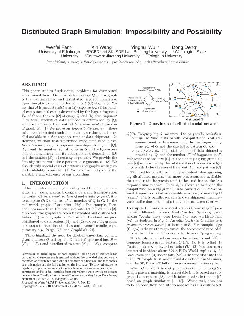
Figure 1: Querying a distributed social network

Q(G). To query big G, we want A to be parallel scalable in◦ response time, if its parallel computational cost (re-

sponse time) is determined only by the largest frag-ment Fm of G and the size |Q| of pattern Q; and

◦ data shipment, if its total amount of data shipped isdecided by |Q| and the number |F| of fragments in F ;

independent of the size |G| of the underlying big graph G;here |G| is measured by the total number of nodes and edgesin G; similarly for the sizes of fragment |Fm| and pattern |Q|.

The need for parallel scalability is evident when queryingbig distributed graphs: the more processors are available,the smaller the fragments tend to be, and hence, the lessresponse time it takes. That is, it allows us to divide thecomputation on a big graph G into parallel computation onsmall fragments of G of manageable sizes, i.e., to make big G“small”. If it is parallel scalable in data shipment, then net-work traffic does not substantially increase when G grows.

Example 1: Consider a social graph G consisting of peo-ple with different interests: Food (f nodes), Sports (sp), andamong Youtube users, beer lovers (yb) and worldcup fans(yf), as depicted in Fig. 1. An edge (A,B) in G indicates atrusted recommendation [19] from A to B. For example, edge(f3, sp2) indicates that sp2 trusts the recommendation of f3for e.g., beer. Graph G is distributed to sites S1, S2 and S3.

To identify potential customers for a beer brand [21], acompany issues a graph pattern Q (Fig. 1). It is to find (1)Youtube users who favor beer ads (YB); (2) Youtube usersinterested in videos about “2014 FIFA World-cup” (YF), (3)Food lovers and (4) soccer fans (SP). The conditions are thatF and YF people trust recommendations from the YB users,and the SP, F and YF folks form a recommendation cycle.

When G is big, it is cost prohibitive to compute Q(G).Graph pattern matching is intractable if it is based on sub-graph isomorphism [33], and it takes quadratic time in |G|based on graph simulation [11, 18]. Worse still, data hasto be shipped from one site to another as G is distributed.

With this comes the need for a parallel scalable algorithmA, to allow a high degree of parallelism and to efficientlyfind potential customers independent of |G|. 2

The practical need raises the following fundamental ques-tions. Is it possible at all to find a distributed algorithmA that is parallel scalable for graph pattern matching? Ifnot, under what conditions such A exists? Are there other(weaker) performance bounds that allow A to scale with|G|? While a number of algorithms have been developedfor distributed pattern matching (e.g., [10, 15, 29, 30]), andseveral distributed graph systems are in place [4,26], to thebest of our knowledge, these questions have not been settled.

Contributions. This paper tackles these questions. Wefocus on graph pattern matching defined with graph sim-ulation [18], as it is commonly used in social communitydetection [7], biological analysis [23], and wireless and mo-bile network analyses [16]. While conventional subgraph iso-morphism often fails to capture meaningful matches, graphsimulation fits into emerging applications with its “many-to-many” matching semantics [7, 11, 18]. Moreover, it is chal-lenging since graph simulation is “recursively defined” andhas poor data locality [9] (see Section 2 about data locality).

The main contributions of the paper are as follows.

(1) We identify desirable performance guarantees for dis-tributed graph pattern matching algorithms (Section 3). Weuse parallel scalability to characterize that the response timeand data shipment are independent of the size of graph G.

(2) No matter how desirable, we show that parallel scala-bility is beyond reach for distributed graph simulation (Sec-tion 3). We prove an impossibility theorem: there exists noalgorithm for distributed graph simulation that is parallelscalable in either its response time or data shipment.

(3) Nonetheless, we identify doable cases for distributedgraph simulation with performance guarantees (Section 4).For patterns Q and distributed graphs G, we provide adistributed simulation algorithm that is partition bounded.That is, its response time depends only on the largest frag-ment Fm of G, the size |Q| of Q, and the number |Vf | ofnodes with edges across different fragments. Better still, itsdata shipment is bounded by O(|Ef ||Q|), where Ef is theset of all crossing edges. In practice |Vf | and |Ef | are typi-cally much smaller than |G|, and |Q| is small. Hence boththe response time and data shipment of the algorithm areoften independent of |G|, i.e., they are not a function of |G|.

(4) When either query Q or graph G is an acyclic directgraph (i.e., a DAG), we show that better bounds exist (Sec-tion 5). We develop a distributed simulation algorithm forDAGs that is parallel scalable in response time under certainconditions. When G is a tree, we give an algorithm thatis parallel scalable in data shipment. To the best of ourknowledge, these are the first distributed graph simulationalgorithms that have these performance bounds.

The bounds of our algorithms are shown in Table 1 (thelast three rows), compared with prior work. They remainintact no matter how graphs are partitioned and distributed.

(5) Using real-life and synthetic graphs, we experimentallyverify the scalability and efficiency of our algorithms. Wefind that our algorithms scale well with graphs G: theirresponse time and data shipment are not a function of |G|.

The algorithms are efficient: they take 21 seconds for cyclicqueries on graphs with 18 million nodes and edges. Ouralgorithms substantially outperform previous algorithms fordistributed graph simulation: on average they are 3.5 and21.6 times faster, and ships 3 and 2 orders of magnitudeless data than those of [25] and [14], respectively. On DAGs,they are 4.7 times faster than the algorithm of [25].

To the best of our knowledge, (1) the results are among thefirst that tell us what is doable and what is undoable for dis-tributed graph simulation. (2) Our algorithms possess thelowest known bounds on response time and data shipment.(3) In addition, the algorithms highlight a new approachfor distributed query processing, by combining partial eval-uation [10, 12, 30] and message passing [22, 26] (see detailsshortly). Taken together with approximation algorithms [27]that minimize |Fm| and |Vf | in graph partitioning, the algo-rithms are a step toward making distributed graph patternmatching scalable with real-life graphs.

Related Work. We categorize related work as follows.

Distributed graph databases. There have been several graphsystems for storing and querying distributed graphs [22,26,36]. Microsoft Trinity [36] is a distributed graph storage and(SPARQL) querying system. Facebook TAO [34] is a geo-graphically distributed system that supports simple graphqueries (e.g., neighborhood retrieval). Below we discuss tworepresentative systems, Pregel [26] and GraphLab [22].

Pregel [26] is a distributed graph system based on synchro-nized message passing. It partitions a graph into clusters,and selects a master machine to assign each cluster to a slavemachine. A graph algorithm is executed in a series of super-steps, during which slave machines send messages to eachother and change their status (voting or halt). The mastermachine communicates with slaves after each superstep, toguide them for the next step. The algorithm terminates if allthe nodes halt. Several graph query algorithms (distance,PageRank, etc.) are supported by Pregel (see [26]).

GraphLab [22] is an asynchronous parallel-computationframework for graphs, optimized for scalable machine learn-ing and data mining algorithms. Given data graph G, a user-defined update function modifies the data attached to thenodes in G, and a sync operation gathers final results. Themajor difference between Pregel and GraphLab is that thelatter decouples the scheduling of computation from messagepassing, by allowing “caching” information at edges.

These frameworks provide system-level optimizations fore.g., usability and scalability. However, it is hard to assureprovable performance bounds in these frameworks, espe-cially for graph pattern matching in arbitrarily partitionedgraphs. (1) Message passing of Pregel may serialize opera-tions that can be conducted in parallel, hence incur excessivenetwork traffic. (2) GraphLab reduces, to some extent, un-necessary messages. However, the improvement is only ver-ified empirically, and highly depends on update and parti-tioning strategy. In fact, we show (Section 3) that the impos-sibility theorem of this work also holds in both frameworks.

Distributed graph query evaluation. Several algorithms havebeen developed for querying distributed graphs with perfor-mance guarantees, via partial evaluation or message passing.Methods based on partial evaluation [10, 12, 15, 25, 29, 30]specify a coordinator site S0 and a set of worker sites. Uponreceiving a query Q, S0 posts Q to workers. Each worker

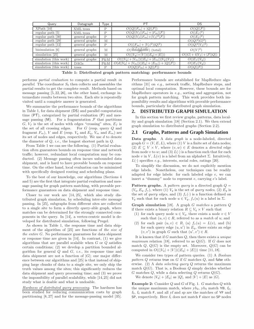
Query Datagraph Type PT DS

XPath [10] XML trees P O(|Q||Fm| + |Q||F|) O(|Q||F|)regular path [5] XML trees P O(|Q||Vf ||Fm|+ |Fm||F|) O(|Ef |

2)regular path [30] general graphs P O(|Q||Vf ||Fm|+|Vf |

2|F|) O(|Ef |2)

regular path [29] general graphs M - O(|Q|2|G|2)regular path [12] general graphs P O((|Fm| + |Vf |

2)|Q|2) O(|Q|2|Vf |2)

bisimulation [6] general graphs M O(|V |2+|V ||E|

|F|) (total) O(|V |2)

simulation [25] general graphs M O((|Vq|+|V |)(|Eq|+|E|)) O(|G|+ 4|Vf |+ |F||Q|)

simulation (this work) general graphs P&M O((|Vq|+ |Vm|)(|Eq |+ |Em|)|Vq ||Vf |) O(|Ef ||Vq|)simulation (this work) DAGs P&M O(d(|Vq | + |Vm|)(|Eq| + |Em|) + |Q||F|) O(|Ef ||Vq|)simulation (this work) trees P O(|Q||Fm| + |Q||F|) O(|Q||F|)

Table 1: Distributed graph pattern matching: performance bounds

performs partial evaluation to compute a partial result inparallel. The coordinator S0 then collects and assembles thepartial results to get the complete result. Methods based onmessage passing [5, 22, 26], on the other hand, exchange in-termediate results between two sites. Each site is repeatedlyvisited until a complete answer is generated.

We summarize the performance bounds of the algorithmsin Table 1, for data shipment (DS) and parallel computationtime (PT), categorized by partial evaluation (P) and mes-sage passing (M). For a fragmentation F that partitionsG, Vf is the set of nodes with edges “crossing” sites, Ef isthe set of all crossing edges. For G (resp. query Q andfragment Fm), V and E (resp. Vq and Eq, Vm and Em) areits set of nodes and edges, respectively. We use d to denotethe diameter of Q, i.e., the longest shortest path in Q.

From Table 1 we can see the following. (1) Partial evalua-tion often guarantees bounds on response time and networktraffic; however, redundant local computation may be con-ducted. (2) Message passing often incurs unbounded datashipment, and is hard to have provable bounds on responsetime. On the other hand, local evaluation can be minimizedwith specifically designed routing and scheduling plans.

To the best of our knowledge, our algorithms (Sections 4and 5) are the first that integrate partial evaluation and mes-sage passing for graph pattern matching, with provable per-formance guarantees on data shipment and response time.

Closer to our work are [14, 25], which also study dis-tributed graph simulation, by scheduling inter-site messagepassing. In [25], subgraphs from different sites are collectedto a single site to form a directly query-able graph, wherematches can be determined for the strongly connected com-ponents in the query. In [14], a vertex-centric model is de-veloped for distributed simulation, following Pregel.

As shown in Table 1, the response time and data ship-ment of the algorithm of [25] are functions of the size ofthe entire G. No performance guarantees for data shipmentor response time are given in [14]. In contrast, (1) we givealgorithms that are parallel scalable when G or Q satisfiescertain conditions; (2) we develop a partition bounded al-gorithm for general Q and G, i.e., its response time anddata shipment are not a function of |G|; one major differ-ence between our algorithms and [25] is that instead of ship-ping large chunks of data to a single site, we only ship thetruth values among the sites; this significantly reduces thedata shipment and query processing time; and (3) we provethe impossibility of parallel scalability, while [14,25] did notstudy what is doable and what is undoable.

Hardness of distributed query processing. The hardness hasbeen studied for reducing communication costs by graphpartitioning [8, 27] and for the message-passing model [35].

Performance bounds are established for MapReduce algo-rithms [31] on e.g., network traffic, MapReduce steps, andoptimal local computation. However, these bounds are forMapReduce operators in e.g., sorting and aggregation, notfor graph pattern matching. This work provides both im-possibility results and algorithms with provable performancebounds, particularly for distributed graph simulation.

2. DISTRIBUTED GRAPH SIMULATIONIn this section we first review graphs, patterns, data local-

ity and graph simulation [18] (Section 2.1). We then extendgraph simulation to distributed graphs (Section 2.2).

2.1 Graphs, Patterns and Graph SimulationData graphs. A data graph is a node-labeled, directedgraph G = (V, E, L), where (1) V is a finite set of data nodes;(2) E ⊆ V × V , where (v, w) ∈ E denotes a directed edgefrom node v to w; and (3) L(·) is a function such that for eachnode v in V , L(v) is a label from an alphabet Σ. Intuitively,L(·) specifies e.g., interests, social roles, ratings [20].

To simplify the discussion, we do not explicitly mentionedge labels. Nonetheless, our techniques can be readilyadapted for edge labels: for each labeled edge e, we caninsert a “dummy” node to represent e, carrying e’s label.

Pattern graphs. A pattern query is a directed graph Q =(Vq, Eq, fv), where (1) Vq is the set of query nodes, (2) Eq isthe set of query edges, and (3) fv(·) is a function defined onVq such that for each node u ∈ Vq , fv(u) is a label in Σ.

Graph simulation [18]. A graph G matches a pattern Qif there exists a binary relation R ⊆ Vq × V such that(1) for each query node u ∈ Vq, there exists a node v ∈ V

such that (u, v) ∈ R, referred to as a match of u; and

(2) for each pair (u, v) ∈ R, (a) fv(u) = L(v), and (b)for each query edge (u, u′) in Eq, there exists an edge(v, v′) in graph G such that (u′, v′) ∈ R.

It is known that if G matches Q, then there exists a uniquemaximum relation [18], referred to as Q(G). If G does notmatch Q, Q(G) is the empty set. Moreover, Q(G) can becomputed in O((|Vq | + |V |)(|Eq| + |E|)) time [11,18].

We consider two types of pattern queries. (1) A Booleanpattern Q returns true on G if G matches Q, and false oth-erwise. (2) A data selecting query Q returns the maximummatch Q(G). That is, a Boolean Q simply decides whetherG matches Q, while a data selecting Q returns Q(G).

We denote |Vq| + |Eq| as |Q|, and |V | + |E| as |G|.

Example 2: Consider Q and G of Fig. 1. G matches Q withthe unique maximum match, where yb2, yb3 match YB, f2,f3, f4 match F, and all yf and sp are the matches of YF andSP, respectively. Here f1 does not match F since no SP nodes

...

G1 G2 Gn

A

B

1

1

A2

B

A2

2

A3

B

An

n

A1

S 1 S 2 S n

A

B

Q0

A1

B1

A2

B2

Bn

An

G0

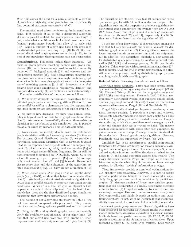
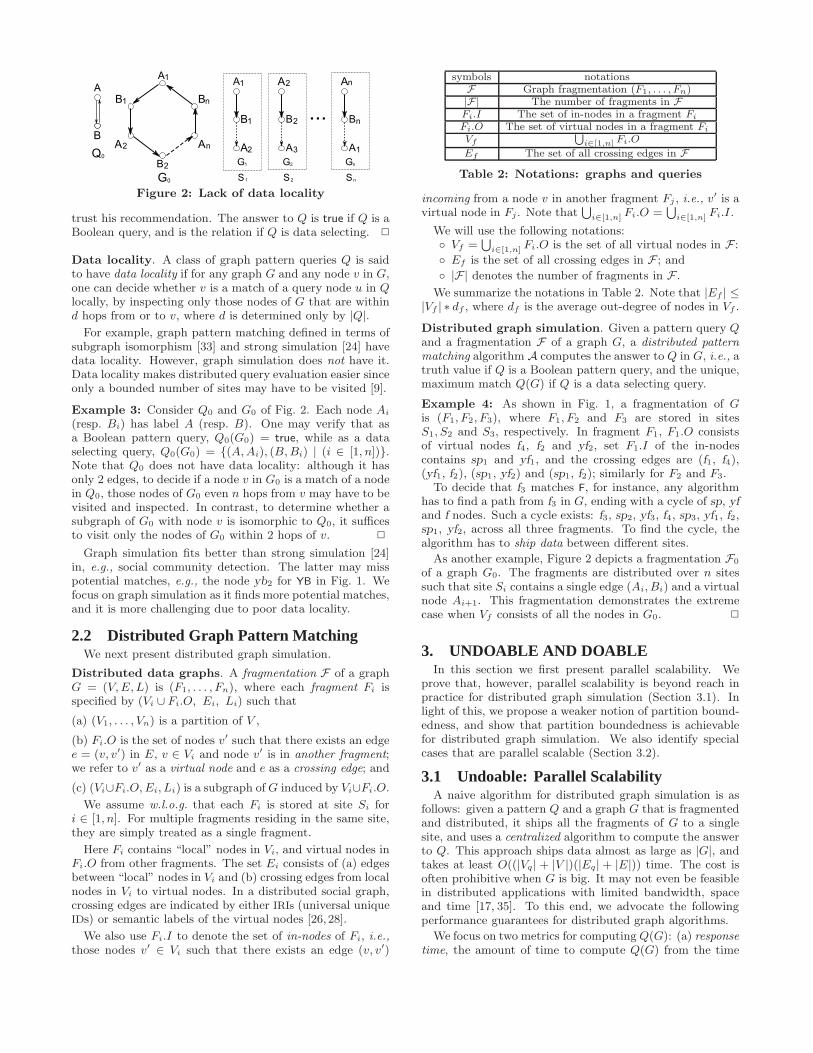
Figure 2: Lack of data locality

trust his recommendation. The answer to Q is true if Q is aBoolean query, and is the relation if Q is data selecting. 2

Data locality. A class of graph pattern queries Q is saidto have data locality if for any graph G and any node v in G,one can decide whether v is a match of a query node u in Qlocally, by inspecting only those nodes of G that are withind hops from or to v, where d is determined only by |Q|.

For example, graph pattern matching defined in terms ofsubgraph isomorphism [33] and strong simulation [24] havedata locality. However, graph simulation does not have it.Data locality makes distributed query evaluation easier sinceonly a bounded number of sites may have to be visited [9].

Example 3: Consider Q0 and G0 of Fig. 2. Each node Ai

(resp. Bi) has label A (resp. B). One may verify that asa Boolean pattern query, Q0(G0) = true, while as a dataselecting query, Q0(G0) = {(A, Ai), (B, Bi) | (i ∈ [1, n])}.Note that Q0 does not have data locality: although it hasonly 2 edges, to decide if a node v in G0 is a match of a nodein Q0, those nodes of G0 even n hops from v may have to bevisited and inspected. In contrast, to determine whether asubgraph of G0 with node v is isomorphic to Q0, it sufficesto visit only the nodes of G0 within 2 hops of v. 2

Graph simulation fits better than strong simulation [24]in, e.g., social community detection. The latter may misspotential matches, e.g., the node yb2 for YB in Fig. 1. Wefocus on graph simulation as it finds more potential matches,and it is more challenging due to poor data locality.

2.2 Distributed Graph Pattern MatchingWe next present distributed graph simulation.

Distributed data graphs. A fragmentation F of a graphG = (V, E, L) is (F1, . . . , Fn), where each fragment Fi isspecified by (Vi ∪ Fi.O, Ei, Li) such that

(a) (V1, . . . , Vn) is a partition of V ,

(b) Fi.O is the set of nodes v′ such that there exists an edgee = (v, v′) in E, v ∈ Vi and node v′ is in another fragment;we refer to v′ as a virtual node and e as a crossing edge; and

(c) (Vi∪Fi.O, Ei, Li) is a subgraph of G induced by Vi∪Fi.O.

We assume w.l.o.g. that each Fi is stored at site Si fori ∈ [1, n]. For multiple fragments residing in the same site,they are simply treated as a single fragment.

Here Fi contains “local” nodes in Vi, and virtual nodes inFi.O from other fragments. The set Ei consists of (a) edgesbetween “local” nodes in Vi and (b) crossing edges from localnodes in Vi to virtual nodes. In a distributed social graph,crossing edges are indicated by either IRIs (universal uniqueIDs) or semantic labels of the virtual nodes [26,28].

We also use Fi.I to denote the set of in-nodes of Fi, i.e.,those nodes v′ ∈ Vi such that there exists an edge (v, v′)

symbols notationsF Graph fragmentation (F1, . . . , Fn)|F| The number of fragments in FFi.I The set of in-nodes in a fragment Fi

Fi.O The set of virtual nodes in a fragment Fi

Vf

S

i∈[1,n] Fi.O

Ef The set of all crossing edges in F

Table 2: Notations: graphs and queries

incoming from a node v in another fragment Fj , i.e., v′ is avirtual node in Fj . Note that

S

i∈[1,n] Fi.O =S

i∈[1,n] Fi.I .

We will use the following notations:◦ Vf =

S

i∈[1,n] Fi.O is the set of all virtual nodes in F :

◦ Ef is the set of all crossing edges in F ; and

◦ |F| denotes the number of fragments in F .

We summarize the notations in Table 2. Note that |Ef | ≤|Vf | ∗ df , where df is the average out-degree of nodes in Vf .

Distributed graph simulation. Given a pattern query Qand a fragmentation F of a graph G, a distributed patternmatching algorithm A computes the answer to Q in G, i.e., atruth value if Q is a Boolean pattern query, and the unique,maximum match Q(G) if Q is a data selecting query.

Example 4: As shown in Fig. 1, a fragmentation of Gis (F1, F2, F3), where F1, F2 and F3 are stored in sitesS1, S2 and S3, respectively. In fragment F1, F1.O consistsof virtual nodes f4, f2 and yf2, set F1.I of the in-nodescontains sp1 and yf1, and the crossing edges are (f1, f4),(yf1, f2), (sp1, yf2) and (sp1, f2); similarly for F2 and F3.

To decide that f3 matches F, for instance, any algorithmhas to find a path from f3 in G, ending with a cycle of sp, yf

and f nodes. Such a cycle exists: f3, sp2, yf3, f4, sp3, yf1, f2,sp1, yf2, across all three fragments. To find the cycle, thealgorithm has to ship data between different sites.

As another example, Figure 2 depicts a fragmentation F0

of a graph G0. The fragments are distributed over n sitessuch that site Si contains a single edge (Ai, Bi) and a virtualnode Ai+1. This fragmentation demonstrates the extremecase when Vf consists of all the nodes in G0. 2

3. UNDOABLE AND DOABLEIn this section we first present parallel scalability. We

prove that, however, parallel scalability is beyond reach inpractice for distributed graph simulation (Section 3.1). Inlight of this, we propose a weaker notion of partition bound-edness, and show that partition boundedness is achievablefor distributed graph simulation. We also identify specialcases that are parallel scalable (Section 3.2).

3.1 Undoable: Parallel ScalabilityA naive algorithm for distributed graph simulation is as

follows: given a pattern Q and a graph G that is fragmentedand distributed, it ships all the fragments of G to a singlesite, and uses a centralized algorithm to compute the answerto Q. This approach ships data almost as large as |G|, andtakes at least O((|Vq | + |V |)(|Eq| + |E|)) time. The cost isoften prohibitive when G is big. It may not even be feasiblein distributed applications with limited bandwidth, spaceand time [17, 35]. To this end, we advocate the followingperformance guarantees for distributed graph algorithms.

We focus on two metrics for computing Q(G): (a) responsetime, the amount of time to compute Q(G) from the time

when Q is issued; and (b) data shipment, the total amountof data shipped between the sites in order to compute Q(G).

Parallel scalability. We say that a distributed graph sim-ulation algorithm A is parallel scalable

◦ in response time if for all patterns Q, graphs G and allfragmentations F of G, its cost for parallelly comput-ing Q(G) is bounded by a polynomial in the sizes |Q|and |Fm|, where Fm is the largest fragment in F ; and

◦ in data shipment if it ships at most a polynomialamount of data in |Q| and |F|, where |F| is the numberof fragments (sites) involved in communication;

both independent of the size of the entire graph G.

If an algorithm is parallel scalable in response time, thenone can partition a big graph and distribute its fragments todifferent processors, such that the more processors are avail-able, the less response time it takes, i.e., this notion aims tocharacterize the degree of parallelism. If an algorithm is par-allel scalable in data shipment, then it scales with |G| whenG grows (note that |F| is typically much smaller than G).

Impossibility theorems. No matter how desirable, how-ever, we show below that it is impossible to find a parallelscalable algorithm for distributed graph simulation.

Theorem 1: There exists no algorithm for distributed graphsimulation that is parallel scalable in (1) either response time(2) or data shipment, even for Boolean pattern queries. 2

Proof sketch: We prove (1) and (2) by contradiction. Forthe lack of space we defer the detailed proof to [3].

(1) Assume that there exists a distributed graph simulationalgorithm A that is parallel scalable in response time. Thenthere exist a Boolean pattern Q0, a graph G0 and a fragmen-tation F0 of G0 of the form shown in Fig. 2 (see Examples 3and 4), such that A does not correctly decide whether G0

matches Q0. Indeed, if A is parallel scalable, then it takesconstant time t when processing Q0 on F0, since |Q0| isa constant, and each fragment of F0 has a constant size.However, F0 has n fragments, for a “variable” n. To decidewhether G0 matches Q0, we show that information has tobe assembled from m sites and analyzed, for t < m ≤ n.

(2) Assume that there exists an algorithm A that is paral-lel scalable in data shipment. We show that there exist aBoolean pattern Q1, a graph G1 and a fragmentation F1

of G1, such that A does not correctly decide whether G1

matches Q1. We use the same Q0 above as Q1, a variationG1 of G0, and an F1 with two fragments, one consisting ofall the A nodes of G1 and the other with all the B nodes.Then only a constant amount c of data can be sent by A,since |Q0| and |F1| are constants. However, we show thatto correctly decide whether G1 matches Q0, data about atleast m nodes has to be sent, where c < m ≤ n, and n is thenumber of nodes in a fragment of F1. 2

Remarks. The result is generic: it holds on distributedmodels in which each site makes decisions based on the mes-sages received and local evaluation, e.g., partial evaluationmodels [10, 12, 30]. It also holds on vertex-centric graphprocessing systems, e.g., Pregel [26] and GraphLab [22],in which each node makes decision on local computationand message sending. One can verify that the proof aboveapplies to vertex-centric computation, regardless of e.g.,how the asynchronous local strategy schedules the messages

(GraphLab), or how a synchronized superstep coordinatesthe shipment of messages (Pregel). See [3] for details.

3.2 Doable: Partition BoundednessTheorem 1 suggests that we consider weaker performance

guarantees for distributed graph simulation.

Partition boundedness. We say that an algorithm A fordistributed graph simulation is partition bounded

◦ in response time if its parallel computation cost is apolynomial function in |Q|, |Fm| and |Vf | (or |Ef |), and

◦ in data shipment if the total data shipped is boundedby a polynomial in |Q| and |Ef | (or |Vf |).

That is, A depends on how G is partitioned, not on itssize |G|. For a partition F (thus fixed |Vf | and |Ef |), neitherits response time nor data shipment is measured in the sizeof G. In practice |Vf | and |Ef | are typically much smallerthan |G|; hence, if A is partition bounded, it often scales wellwith big G. In addition, approximation graph partitioningmethods are already in place [27] to minimize |Vf | and |Ef |,possibly making the sizes of Vf and Ef independent of |G|.

Positive results. Despite Theorem 1, we show that it isstill possible to find efficient algorithms for distributed graphsimulation with performance guarantees.

Theorem 2: There exists an algorithm for distributed graphsimulation that is partition bounded in both response timeand data shipment. Over any fragmentation F of a graphG, it evaluates a pattern query Q = (Vq, Eq, fv)

◦ in O(|Vf ||Vq |(|Vq | + |Vm|)(|Eq| + |Em|)) time, and

◦ ships at most O(|Ef ||Vq |) amount of data,where Fm = (Vm, Em, Lm) is the largest fragment in F. 2

When either Q or G is a directed acyclic graph (i.e., DAG),we have better bounds, and moreover, parallel scalability inresponse time when the number |F| of fragments is fixed.

Theorem 3: When either graph G or pattern Q is a DAG,there exists an algorithm that computes Q(G)

◦ in O(d(|Vq | +|Vm|)(|Eq| + |Em|) + |Q||F|) time, and

◦ ships at most O(|Ef ||Vq |) amount of data,where d is the diameter of Q, and F is a fragmentation ofG. If |F| is fixed, it is parallel scalable in response time. 2

When G is a tree, parallel scalability is achievable in datashipment, and furthermore, possible in response time when|F| is fixed. The bounds below are the same as those for eval-uating XPath queries on distributed XML trees [10]. Thatis, we show that the bounds of [10] on XPath extend todistributed graph simulation on trees.

Corollary 4: When G is a tree and each fragment of F isconnected, there exists a parallel scalable algorithm in datashipment. More specifically, it (a) is in O(|Q||Fm|+ |Q||F|)time, and (b) ships at most O(|Q||F|) amount of data. If|F| is fixed, it is also parallel scalable in response time. 2

We will prove Theorem 2 in Section 4, and Theorem 3 andCorollary 4 in Section 5, by providing such algorithms.

Remarks. (1) Our performance bounds and techniques donot require any particular fragmentation strategy, while theywork better on fragmentations that minimize |Vf | and |Ef |.

(2) Table 1 shows that only the algorithms of [10] guaran-tee parallel scalability in data shipment. Those of [5,12,30]

are partition bounded in data shipment, and among these,only [12] is partition bounded in response time. Thesealgorithms are for either XML trees [5] or regular pathqueries [12, 30]. Distributed graph simulation is more chal-lenging, and we are not aware of any prior algorithms for dis-tributed graph simulation that are partition bounded. Thealgorithms of [6, 25], for instance, require to ship data ofO(|G|) size, i.e., the entire graph, and take as much time asthe naive algorithm given above in the worst case.

4. PARTITION BOUNDED ALGORITHMSIn this section we prove Theorem 2 by developing an al-

gorithm for distributed graph simulation with the desiredbounds. In contrast to conventional distributed algo-rithms, the algorithm leverages both partial evaluation andmessage passing. (1) As opposed to partial evaluation, itadopts asynchronous message passing to direct partial re-sults among fragments. (2) In contrast to vertex-centricmodels (e.g., Pregel, GraphLab) where each node has a com-puting node for local computation, it conducts local evalu-ation on a fragment with effective optimization.

We first present a baseline algorithm in Section 4.1, andthen improve it with optimization techniques in Section 4.2.

4.1 Algorithm for Graph SimulationWe start with the baseline algorithm, denoted as dGPM.

We first study data selecting queries, and then Boolean ones.

Algorithm dGPM uses partial evaluation to compute par-tial answers on a fragment at each local site in parallel. Eachsite then refines its partial answer upon receiving messagesfrom others, and sends updated answers to others, guidedby the dependency among the sites, i.e., whether a site needsthe values of its virtual nodes from other sites. The processrepeats until no change happens at any site.

We first present auxiliary structures used by dGPM. Con-sider Q = (Vq, Eq, Lq), G = (V, E, L), and a fragmentationF = (F1, . . . , Fn) of G, where each Fi is stored at site Si.

Partial answers. A straightforward way to define partialanswer for a site Si is to induce the subgraph of Fi from allthe candidate nodes, assuming that they are all matches [25].However, this incurs unbounded data shipment. Instead ofshipping data of Fi, we send Boolean variables denoting par-tial results of Q on local fragment Fi, defined as follows.

(a) With each node v in Fi and each pattern node u in Q,we associate a Boolean variable X(u,v) to indicate whetherv is a match of u. All such variables for v form a Booleanvector v.rvec of size |Vq|, for all pattern nodes u in Q.

(b) A partial answer is a set Li of vectors v.rvec consistingof all the in-nodes v in Fi, such that v.rvec[u] is defined bya Boolean formula only in terms of the Boolean variables ofthe virtual nodes in Fi. We say that v is unevaluated for uif the truth value of X(u,v) is not yet known.

Local dependency graphs. A local dependency graphat site Si keeps track of all the sites with virtual nodes asin-nodes at Si, More specifically, each site Si stores a localdependency graph Gi

d = (V id , Ei

d, Aid), where

◦ each node Sj in V id represents a site,

◦ there is an edge (Sj , Si) in Eid if there is a virtual node

vj in Fj as an in-node in Fi; and

coordinator

site 1

site 2

site k...

1. pattern query 1. pattern query

1. pattern

query

3. partial

matches

3. partial

matches

3. partial

matches

1. (incremental)

partial evaluation

2. message passing

local dependency graph

site 1

site 2

...2.partial

results

Figure 3: Distributed pattern matching: framework

◦ a function Aid(·) on Ed such that for each edge

(Sj , Si), Aid(Sj , Si) is the set of all virtual nodes vj in

Fj (resp. in-nodes in Fi) as described above.

Such a Gid is determined by fragmentation F only and is

small. Each site Si can compute Gid offline in parallel, by

sharing the identifiers of its virtual and in-nodes [26,28] withother sites, using hashing [26] or indexing techniques [36].

Example 5: Consider Q and G of Fig. 1. Each site Si keepsa local dependency graph Gi

d. For site S3, G3d contains edges

(S1, S3) (annotated with f4) and (S2, S3) (annotated with{sp3, yf3}), as site S1 has a virtual node f4 as an in-nodein S3; similarly for S2. A partial answer at e.g., site S3 is aset of Boolean vectors, one for each of its in-nodes sp3, yf3and f4. For, e.g., sp3, the truth value of an entry X(SP,sp1)

in its associated vector indicates if sp3 is a match for SP. 2

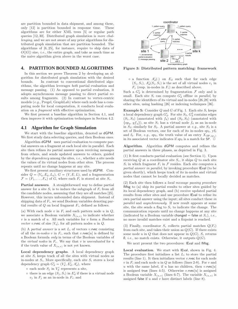
Algorithm. Algorithm dGPM computes and refines thepartial answers in three phases, as depicted in Fig. 3.

(1) It first conducts partial evaluation (see Section 1). Uponreceiving Q at a coordinator site Sc, it ships Q to each siteSi in which fragment Fi in F resides. Each site computes apartial answer in parallel, by invoking procedure lEval (to begiven shortly), which keeps track of its in-nodes and virtualnodes that cannot be locally decided as matches.

(2) Each site then follows a local message passing procedurelMsg to (a) ship its partial results to other sites guided byits local dependency graph, and (b) receive updated partialresults from other sites and use procedure lEval to refine itsown partial answer using the input; all sites conduct these inparallel and asynchronously. If new result appears at somesite, the site sends a flag to Sc to indicate the change. Thecommunication repeats until no change happens at any site(indicated by a Boolean variable changed = false at Sc), i.e.,no more invalid matches exist and a fixpoint is reached.

(3) Finally, coordinator Sc collects partial matches Q(Fi)from each site, and takes their union as Q(G). If there existssome node u in Q that does not appear in Q(G), Sc returns∅, i.e., no match exists. Otherwise, it outputs Q(G).

We next present the two procedures: lEval and lMsg.

Local evaluation. We start with lEval, shown in Fig. 4.The procedure first initializes a list Li to store the partialresults (line 1). It then initializes vector v.rvec for each nodev in Fi and each node u in Q as follows (lines 2-8). For v andu with the same label, if u has no children, then v.rvec[u]is assigned true (lines 4-5). Otherwise v.rvec[u] is assigneda Boolean variable X(u,v) (lines 6-7). The variable X(u,v) isassigned false if u and v have distinct labels (line 8).

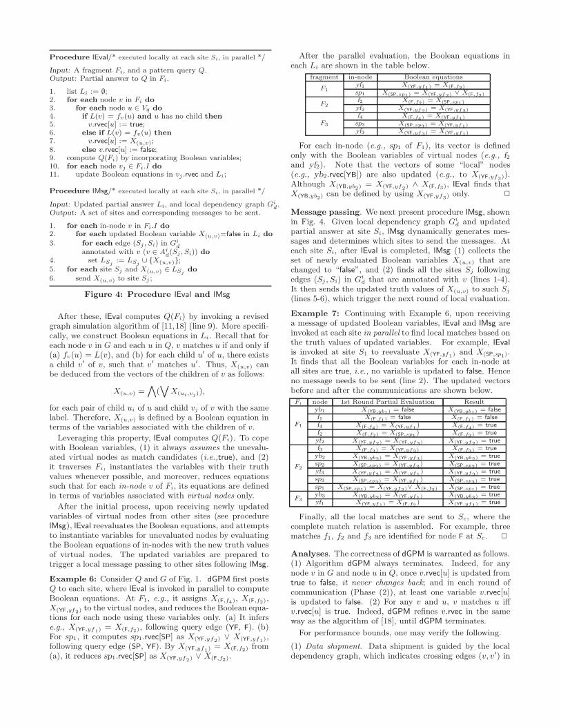
Procedure lEval/* executed locally at each site Si, in parallel */

Input: A fragment Fi, and a pattern query Q.Output: Partial answer to Q in Fi.

1. list Li := ∅;2. for each node v in Fi do

3. for each node u ∈ Vq do

4. if L(v) = fv(u) and u has no child then

5. v.rvec[u] := true;6. else if L(v) = fv(u) then

7. v.rvec[u] := X(u,v);8. else v.rvec[u] := false;9. compute Q(Fi) by incorporating Boolean variables;10. for each node vj ∈ Fi.I do

11. update Boolean equations in vj .rvec and Li;

Procedure lMsg/* executed locally at each site Si, in parallel */

Input: Updated partial answer Li, and local dependency graph Gid.

Output: A set of sites and corresponding messages to be sent.

1. for each in-node v in Fi.I do

2. for each updated Boolean variable X(u,v)=false in Li do

3. for each edge (Sj , Si) in Gid

annotated with v (v ∈ Aid(Sj , Si)) do

4. set LSj:= LSj

∪ {X(u,v)};5. for each site Sj and X(u,v) ∈ LSj

do

6. send X(u,v) to site Sj ;

Figure 4: Procedure lEval and lMsg

After these, lEval computes Q(Fi) by invoking a revisedgraph simulation algorithm of [11,18] (line 9). More specifi-cally, we construct Boolean equations in Li. Recall that foreach node v in G and each u in Q, v matches u if and only if(a) fv(u) = L(v), and (b) for each child u′ of u, there existsa child v′ of v, such that v′ matches u′. Thus, X(u,v) canbe deduced from the vectors of the children of v as follows:

X(u,v) =^

(_

X(ui,vj)),

for each pair of child ui of u and child vj of v with the samelabel. Therefore, X(u,v) is defined by a Boolean equation interms of the variables associated with the children of v.

Leveraging this property, lEval computes Q(Fi). To copewith Boolean variables, (1) it always assumes the unevalu-ated virtual nodes as match candidates (i.e.,true), and (2)it traverses Fi, instantiates the variables with their truthvalues whenever possible, and moreover, reduces equationssuch that for each in-node v of Fi, its equations are definedin terms of variables associated with virtual nodes only.

After the initial process, upon receiving newly updatedvariables of virtual nodes from other sites (see procedurelMsg), lEval reevaluates the Boolean equations, and attemptsto instantiate variables for unevaluated nodes by evaluatingthe Boolean equations of in-nodes with the new truth valuesof virtual nodes. The updated variables are prepared totrigger a local message passing to other sites following lMsg.

Example 6: Consider Q and G of Fig. 1. dGPM first postsQ to each site, where lEval is invoked in parallel to computeBoolean equations. At F1, e.g., it assigns X(F,f4), X(F,f2),X(YF,yf2) to the virtual nodes, and reduces the Boolean equa-tions for each node using these variables only. (a) It inferse.g., X(YF,yf1) = X(F,f2), following query edge (YF, F). (b)For sp1, it computes sp1.rvec[SP] as X(YF,yf2) ∨ X(YF,yf1),following query edge (SP, YF). By X(YF,yf1) = X(F,f2) from(a), it reduces sp1.rvec[SP] as X(YF,yf2) ∨ X(F,f2).

After the parallel evaluation, the Boolean equations ineach Li are shown in the table below.

fragment in-node Boolean equations

F1yf1 X(YF,yf1) = X(F,f2)

sp1 X(SP,sp1) = X(YF,yf2) ∨ X(F,f2)

F2f2 X(F,f2) = X(SP,sp1)

yf2 X(YF,yf2) = X(YF,yf3)

F3

f4 X(F,f4) = X(YF,yf1)

sp3 X(SP,sp3) = X(YF,yf1)

yf3 X(YF,yf3) = X(YF,yf1)

For each in-node (e.g., sp1 of F1), its vector is definedonly with the Boolean variables of virtual nodes (e.g., f2and yf2). Note that the vectors of some “local” nodes(e.g., yb2.rvec[YB]) are also updated (e.g., to X(YF,yf3)).Although X(YB,yb2) = X(YF,yf2) ∧ X(F,f3), lEval finds thatX(YB,yb2) can be defined by using X(YF,yf3) only. 2

Message passing. We next present procedure lMsg, shownin Fig. 4. Given local dependency graph Gi

d and updatedpartial answer at site Si, lMsg dynamically generates mes-sages and determines which sites to send the messages. Ateach site Si, after lEval is completed, lMsg (1) collects theset of newly evaluated Boolean variables X(u,v) that arechanged to “false”, and (2) finds all the sites Sj followingedges (Sj , Si) in Gi

d that are annotated with v (lines 1-4).It then sends the updated truth values of X(u,v) to such Sj

(lines 5-6), which trigger the next round of local evaluation.

Example 7: Continuing with Example 6, upon receivinga message of updated Boolean variables, lEval and lMsg areinvoked at each site in parallel to find local matches based onthe truth values of updated variables. For example, lEval

is invoked at site S1 to reevaluate X(YF,yf1) and X(SP,sp1).It finds that all the Boolean variables for each in-node atall sites are true, i.e., no variable is updated to false. Henceno message needs to be sent (line 2). The updated vectorsbefore and after the communications are shown below.

Fi node 1st Round Partial Evaluation Result

F1

yb1 X(YB,yb1) = false X(YB,yb1) = false

f1 X(F,f1) = false X(F,f1) = false

f4 X(F,f4) = X(YF,yf1) X(F,f4) = true

f2 X(F,f2) = X(SP,sp1) X(F,f2) = true

yf2 X(YF,yf2) = X(YF,yf3) X(YF,yf2) = true

F2

f3 X(F,f3) = X(YF,yf3) X(F,f3) = true

yb2 X(YB,yb2) = X(YF,yf3) X(YB,yb2) = true

sp2 X(SP,sp2) = X(YF,yf3) X(SP,sp2) = true

yf3 X(YF,yf3) = X(YF,yf1) X(YF,yf3) = true

sp3 X(SP,sp3) = X(YF,yf1) X(SP,sp3) = true

sp1 X(SP,sp1) = X(YF,yf2)∨ X(F,f2) X(SP,sp1) = true

F3yb3 X(YB,yb3) = X(YF,yf1) X(YB,yb3) = true

yf1 X(YF,yf1) = X(F,f2) X(YF,yf1) = true

Finally, all the local matches are sent to Sc, where thecomplete match relation is assembled. For example, threematches f1, f2 and f3 are identified for node F at Sc. 2

Analyses. The correctness of dGPM is warranted as follows.(1) Algorithm dGPM always terminates. Indeed, for anynode v in G and node u in Q, once v.rvec[u] is updated fromtrue to false, it never changes back; and in each round ofcommunication (Phase (2)), at least one variable v.rvec[u]is updated to false. (2) For any v and u, v matches u iffv.rvec[u] is true. Indeed, dGPM refines v.rvec in the sameway as the algorithm of [18], until dGPM terminates.

For performance bounds, one may verify the following.

(1) Data shipment. Data shipment is guided by the localdependency graph, which indicates crossing edges (v, v′) in

Ef , where v′ is both a virtual node in fragment Fi and an in-node in another fragment Fj . The edge is followed only whenv′.rvec[u] is changed to false for some u ∈ Vq, at most |Vq |times. Moreover, each v′.rvec[u] is changed at most once.Hence the total data shipment is bounded by O(|Ef ||Vq |) inall rounds of communications in the worst case.

(2) Response time. In each round of communication, localmatching takes at most t = O((|Vq| + |Vm|)(|Eq| + |Em|))time [11, 18], and there are at most O(|Vf ||Vq |) rounds.In the final step, it takes O(|Vq ||F|) time to merge allthe matches and check whether every query node has amatch from a site. Hence the worst-case response time is inO((|Vq |+ |Vm|) (|Eq|+ |Em|) |Vq ||Vf | + |Vq|F|). In practice,|F| ≤ |Vf |, since fragments are typically not isolated, andeach fragment yields at least one distinct node in Vf . Hence,the overall time complexity is in O((|Vq |+|Vm|) (|Eq|+|Em|)|Vq ||Vf |). Moreover, |Q| (i.e., |Vq |, |Eq|) is typically small,and |Fm| is much smaller than |G| when |F| is large.

Boolean queries. Algorithm dGPM processes Booleanqueries Q by following the same steps (1) and (2) as for dataselecting queries. The only difference is that in step (3), Sc

simply checks whether each node of Q has a match in anylocal site. It returns true if so, and false otherwise.

This completes the proof of Theorem 2.

4.2 Optimization StrategiesWe next introduce two optimization strategies. The first

one reduces unnecessary computation of lEval following theidea of incremental pattern matching [13], upon receivinga message with updated Boolean variables. The second oneenables tunable performance of dGPM between data ship-ment and response time, by allowing a site to send not onlyevaluated Boolean variables, but also Boolean equations.

Incremental local evaluation. Recall that in Phase (2)of dGPM, when a site Si receives a message from anothersite with evaluated values X(u,v) for some virtual node v ofSi, it calls procedure lEval to revise its local matches Q(Fi).

A better idea is to conduct lEval incrementally. It onlypropagates updated truth values, following a “bottom-up”traversal starting from virtual nodes v, and updates the vec-tors of the “ancestors” of v. When it reaches a node v′ withan unchanged vector, it stops the traversal at v′. Finally, ifno vector changes in the entire process, lEval sends false tocoordinator Sc. Otherwise, it sends true to Sc. It also sendsmessages with those X(u,v) for all v ∈ Fi.I that are updatedto false, guided by its local dependency graph.

Following [13], one can verify that this incremental versionof lEval takes optimally O(|AFF|) time to update all matches,where AFF is the set of changed variables, the “area” thatmust be visited in response to the changes. This strategyallows us to minimize unnecessary recomputation.

Example 8: Consider Q and G′ by removing the edge (f2,sp1) from G (Example 6). After partial evaluation, X(F,f2)

is updated to false and sent from S2 to S1. Upon receivingX(F,f2), instead of recomputing all the Boolean formulas,lEval incrementally updates those affected by X(F,f2) startingfrom virtual node f2. It updates X(YF,yf1) to false, followingX(YF,yf1) = X(F,f2) (see Example 6). Similarly, X(SP,sp1) =X(YF,yf2)∨ X(F,f2) is reduced to X(SP,sp1) = X(YF,yf2). Asno new variables can be updated to false, S1 terminates thelocal evaluation, and sends the updated X(YF,yf1) to S3. 2

Tunable message passing strategy. In Phase (2) ofdGPM, a site may do nothing but wait for evaluated vari-ables from its children. To reduce the waiting time andhence, improve the overall response time, we introduce apush operation that allows a site Si to send Boolean equa-tions to another site Sj , instead of Boolean variables, suchthat Sj can “inline” these equations in the equations of itsin-nodes, and hence bypass message passing from Si to Sj .

Push operation. We first extend the local dependency graph

Gid of Si by including the edges (Si, Sk), for all sites Sk

having in-nodes as the virtual nodes in Si. Given Gid at site

Si, a push operation does the following. (1) At site Si, foreach in-node v in Fi, it sends the equations in v.rvec[u] to allthe parent sites Sj in Gi

d if Aid(Sj , Si) contains v, i.e., Sj has

an unevaluated virtual node as in-node v of Si. Site Si alsosends all its children sites Sk in Gi

d to Sj that contributevirtual nodes to the evaluation of v. (2) Each parent Sj

(resp. child Sk) of Si then updates its dependency graphby replacing (Sj , Si) (resp. (Si, Sk)) with edges (Sj , Sk), forsuch child sites Sk (resp. parent site Sj) of Si. Intuitively,this operation outsources part of computation at Si to Sj ,and bypasses the communication via edge (Sj , Si).

To determine when to perform a push operation, site Si

checks whether a benefit function B(Si) exceeds a thresholdθ. The function B(Si) is defined as follows:

B(Si) =|Fi.O

′|

m ∗ |Fi.I ′|where Fi.I

′ (resp. Fi.O′) denotes the number of unevaluated

in-nodes (resp. virtual nodes) at Si, and m denotes the to-tal size of the equations (messages) to be sent. Intuitively,(1) the more unevaluated virtual nodes and the less uneval-uated in-nodes at Si, the longer a parent Sj has to wait formessages from Si, and hence, the better if Si ships its localcomputation to Sj , bypassing Si; and (2) the less amount ofdata requires to be sent, the better a push operation is. IfB(Si) ≥ θ, procedure lMsg triggers a push operation at Si.

Remarks. A push operation ships more data in exchangefor better waiting time. To strike a balance, we use m inB(·) to suppress the overhead of shipment. While waitingtime is the bottleneck in response time (as observed in ourexperiments; see [3]), B(·) can be adjusted (e.g., to be pos-itively correlated with m) to balance local evaluation time.That is, lMsg outsources more computation via push oper-ations for larger m. Other performance metrics (e.g., sitevisit times, workload and processing capacity) can also beintegrated into B(·) to improve the performance of dGPM.

Our experimental study shows that these two optimiza-tion strategies substantially improve the performance. In-deed, dGPM extended with these strategies (also denoted bydGPM) is 20 times faster than its counterpart without them(denoted as dGPMNOpt) on average (see Section 6).

5. PARALLEL SCALABLE ALGORITHMSWe next prove Theorem 3 and Corollary 4 by giving dis-

tributed graph simulation algorithms for DAGs and trees inSections 5.1 and 5.2, respectively, with the desired bounds.

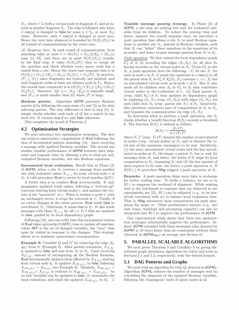
5.1 DAG Patterns and GraphsWe start with an algorithm for DAG Q, denoted as dGPMd.

Algorithm dGPMd reduces the number of messages sent byscheduling the shipment of the updated Boolean variables,following the (topological) ranks of query nodes in Q.

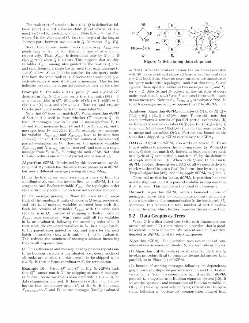
The rank r(u) of a node u in a DAG Q is defined as fol-lows: (a) r(u) = 0 if u has no child; (b) otherwise, r(u) =max(r(u′)) +1 for each child u′ of u. Note that 0 ≤ r(u) ≤ d,where d is the diameter of Q, i.e., the length of the longestshortest path between two nodes in Q. Moreover, d ≤ |Eq|.

Recall that for each node v in G and u in Q, X(u,v) de-pends only on X(u′,v′) for children u′ and v′ of u and v,respectively. Thus, X(u,v) is determined only by X(u′,v′) ifr(u) ≥ r(u′) when Q is a DAG. This suggests that we shipvariables X(u,v) among sites guided by the rank r(u) of u,and send them in a single batch, such that each message tosite Si allows Si to find the matches for the query nodesthat have the same rank r(u). Observe that since r(u) ≤ d,each site sends at most d batches of messages. This furtherindicates less number of partial evaluation over all the sites.

Example 9: Consider a DAG query Q′′ and a graph G′′

depicted in Fig. 5. One may verify that the rank r(FB) = 0as it has no child in Q′′. Similarly, r(YB2) = 1, r(SP) = 2,r(YF) = r(F) = 3, and r(YB1) = 4. Here YB1 and YB2 aretwo distinct query nodes with the same label YB.

Note that G′′ does not match Q′′. When algorithm dGPM

of Section 4 is used to check whether G′′ matches Q′′, intotal 12 messages have to be sent: 2 messages from F4 toF7 and F8, 4 messages from F7 and F8 to F5 and F6, and 6messages from F5 and F6 to F4. For example, two messagesfor variables X(SP,sp4) and X(SP,sp5) have to be sent fromF7 to F5. This further triggers two rounds of (incremental)partial evaluation on F5. However, the updated variablesX(SP,sp4) and X(SP,sp5) can be “merged” and sent as a singlemessage from F7 to F5, following the rank of SP. Note thatthis also reduces one round of partial evaluation at F5. 2

Algorithm dGPMd. Motivated by this observation, we de-velop dGPMd, which has the same three phases as in dGPM,but uses a different message passing strategy lMsgd.

(1) In the first phase, upon receiving a query Q from thecoordinator Sc, each site invokes lEval as in dGPM. It thenassigns to each Boolean variable X(u,v) the topological orderr(u) of the query node u, for each virtual node and in-node v.

(2) For message passing in Phase (2), each site Si keepstrack of the topological ranks of nodes in Q being processed,and lists Lr of updated variables collected from each site.Each list consists of variables X(u,v) with the same rankr(u) for u in Q. Instead of shipping a Boolean variableX(u,v) once evaluated, lMsgd waits until all the variablesin Lr are evaluated, following the ascending order of r. Itthen sends the evaluated variables in Lr, in a single batch,to the parent sites guided by Gi

d, and waits for the nextbatch of variables (i.e., with rank r + 1) to be evaluated.This reduces the numbers of messages without increasingthe overall response time.

(3) This refinement and message passing process repeats un-til no Boolean variable is unevaluated, i.e., query modes ofall ranks are checked (no data needs to be shipped whenr = d). It then informs coordinator Sc for termination.

Example 10: Given Q′′ and G′′ in Fig. 5, dGPMd findsthat Q′′ cannot match G′′ by shipping at most 6 messagesas follows. As no variable is associated with FB (r = 0), nodata shipment is incurred. It then starts with r = 1. Follow-ing the local dependency graph G4

d at site S4, it ships onlyX(YB2,yb4) to F7 and F8, as two messages (locally evaluated

SP

FYF

Q''

YB

YB

G''Sc

FB

yb

yf4

yf5

f6

f5

yf6f7

sp5 sp6

F5

F4

F64

F8F7

sp4 sp7

F7 F8

F5 F6

r=2

r=3

r=4F4

F4r=1

1

2

Figure 5: Scheduling data shipment

as false). After the local evaluation, the variables associatedwith SP nodes in F7 and F8 are all false, where the local rankr = 2 at both sites. Since no more variables are unevaluatedfor query nodes with topological rank 2 at this time, S7 andS8 send these updated values as two messages to F5 and F6,for r = 2. Sites S5 and S6 collect all the variables of querynodes ranked at 3, i.e.,YF and F, and send them to S4, againin two messages. Now at S4, X(YB1,yb4) is evaluated false. Intotal 6 messages are sent, as opposed to 12 by dGPMt. 2

Analyses. Algorithm dGPMd computes Q(G) in O(d(|Vq|+|Vm|) (|Eq| + |Em|) + |Q||F|) time. To see this, note that(a) it performs d rounds of parallel partial evaluation, (b)each round of evaluation takes O((|Vq |+ |Vm|) (|Eq|+ |Em|))time, and (c) it takes O(|Q||F|) time for the coordinator Sc

to merge and assembles Q(G). Further, the bound on thetotal data shipped by dGPM carries over to dGPMd.

DAG G. Algorithm dGPMd also works on acyclic G. To seethis, it suffices to consider the following cases. (a) When Q iscyclic, G does not match Q. Indeed, at least one query nodein a cycle of Q cannot find a match in G, by the definitionof graph simulation. (b) When both Q and G are DAGs,dGPMd applies. Hence given a DAG G, all we need to do is tocheck whether Q is also a DAG (in linear time by using, e.g.,Tarjan’s algorithm [32]), and if so, apply dGPMd to Q and G.

These tell us that for DAGs, dGPMd is partition boundedin data shipment, and it is parallel scalable in response timeif |F| is fixed. This completes the proof of Theorem 3.

Remark. Algorithm dGPMd sends a bounded number ofmessages, hence with low communication cost in applica-tions where site-to-site communication is the bottleneck [35].Moreover, this reduces the total number of partial evalua-tion at the sites, which further improves the response time.

5.2 Data Graphs as TreesWhen G is a distributed tree (with each fragment a con-

nected subtree of G), there exists an algorithm that is paral-lel scalable in data shipment. We present such an algorithm,denoted as dGPMt, for data selecting queries.

Algorithm dGPMt. The algorithm uses two rounds of com-munications between coordinator Sc and each site as follows.

(1) Algorithm dGPMt posts Q to all sites Si. Each site Si

invokes procedure lEval to compute the partial answer Li inparallel, as in Phase (1) of dGPM.

(2) Instead of sending messages following its dependencygraph, each site ships the partial answer Li and the Booleanvector of its “root” to coordinator Sc. Algorithm dGPMt

puts all Li’s together as a Boolean equation system [10]. Itsolves the equations and instantiates all Boolean variables inO(|Q||F|) time by iteratively unifying variables in the equa-tions, following a “bottom-up” computation induced from

the tree fragments, where the variables associated with vir-tual nodes are connected to the variables of in-node theydefine. This completes the first round of communication.

(3) The instantiated Boolean variables are sent back to eachsite, where lEval is invoked again to complete the matchingprocess. After this, each site sends its local matches to Sc,which are assembled at Sc to get answer Q(G), as in dGPM.

Analysis. Observe the following. (1) Each site is visited atmost twice by dGPMt. (2) lEval computes the partial answerat each fragment Fi in O(|Q||Fi|) time. Hence, the total par-allel computational cost of dGPMt is in O(|Q||Fm|). The to-tal response time, including the time for evaluating Booleanequations, is in O(|Q||Fm|+ |Q||F|). (3) Each fragment hasat most a single in-node. Hence, dGPMt ships at most asingle Boolean vector of size O(|Q|) for each fragment, andthe total data shipment is in O(|Q||F|). Note that the linearbound on Boolean equations does not hold when G is a DAG

or a cyclic graph, i.e., the idea only works for trees.

Algorithm dGPMt extends the idea of partial evaluationof XPath queries on fragmented XML trees [10] to graphsimulation on distributed trees, as well as its performancebounds. This completes the proof of Corollary 4.

6. EXPERIMENTAL EVALUATIONWe next present an experimental study of our distributed

algorithms. Using real-life and synthetic graphs, we con-ducted three sets of experiments to evaluate the efficiencyand data shipment of algorithms (1) dGPM, for general pat-tern queries and data graphs; (2) dGPMd, for DAG queries orgraphs; and (3) the scalability of dGPM over large syntheticgraphs. More experimental results are reported in [3].

Experimental setting. We used two real-life graphs.

(1) Real-world graphs. (a) Yahoo (http://webscope.

sandbox.yahoo.com/catalog.php?datatype=g), which has3M nodes and 15M edges. Each node denotes a Web pagewith attributes such as domain. An edge from x to y in-dicates that x links to y. Its size is 1.6GB. (b) Citation(http://www.arnetminer.org/citation/) has 1.4M nodesand 3M edges, in which nodes represent papers with at-tributes such as title, authors, year and venue, and edgesdenote citations. It is a DAG of 628MB.

(2) Synthetic data. We designed a generator to produce

synthetic graphs G = (V, E, L), controlled by the numbersof nodes |V | and edges |E|, where L is taken from a set Σof 15 labels. We use (|V |, |E|) to denote the size of G.

In all our tests we used data selecting patterns.

(2) Graph fragmentation. We randomly partitioned G into

a set F of fragments, controlled by size(F), the average sizeof the fragments. Unless stated otherwise, the size |Fm| ofthe largest fragment is size(F) = |G|/|F|. To control |Vf |(resp. |Ef |), we iteratively “swapped” two nodes in differentfragments that maximally reduced |Vf | (resp. |Ef |) follow-ing [27], until the ratio |Vf |/|V | (resp. |Ef |/|E|) reached athreshold. We represent the size of Vf by the ratio |Vf |/|V |.

(3) Algorithms. We implemented the following algorithms,

all in Java: (1) dGPM (Section 4.1); (2) dGPMd (Section 5);(3) Match, which first ships all fragments to a site, and thencomputes Q(G) using a centralized graph simulation algo-rithm (see Section 3.1); (4) algorithm disHHK of [25]; and

(5) dGPMNOpt, a version of dGPM without using incrementalevaluation or push operations (Section 4.2), to evaluate theeffectiveness of our optimization strategy.

We also developed a message-based algorithm dMes, tosimulate the vertex-centric model of Pregel [14, 26]. Uponreceiving Q from a coordinator Sc, each site Si, as a worker,does the following (as a superstep [14]) for each virtual nodein fragment Fi. (1) It requests the Boolean values from othersites for the variables of its virtual nodes. (2) It performslocal evaluation to update all its local variables. (3) If nochange happens, it sends a flag to Sc to vote for termination.It collects the matches from all the sites if at a superstep,all the sites vote to “terminate”. For a fair comparison, wedo not assume message passing for local evaluation.

Machines. We deployed these algorithms on Amazon EC2General Purpose instances [1]. Each site stored a fragment.Each experiment was run 5 times and the average isreported here. We report the response time (PT) and datashipment (DS) of the algorithms. As dGPMNOpt has the samedata shipment as dGPM, we do not show DS for dGPMNOpt.We do not show DS for Match as it always ships the entireG. We fixed threshold θ for push operations at 0.2.

Experimental results. We next report our findings.

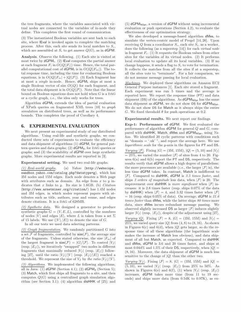
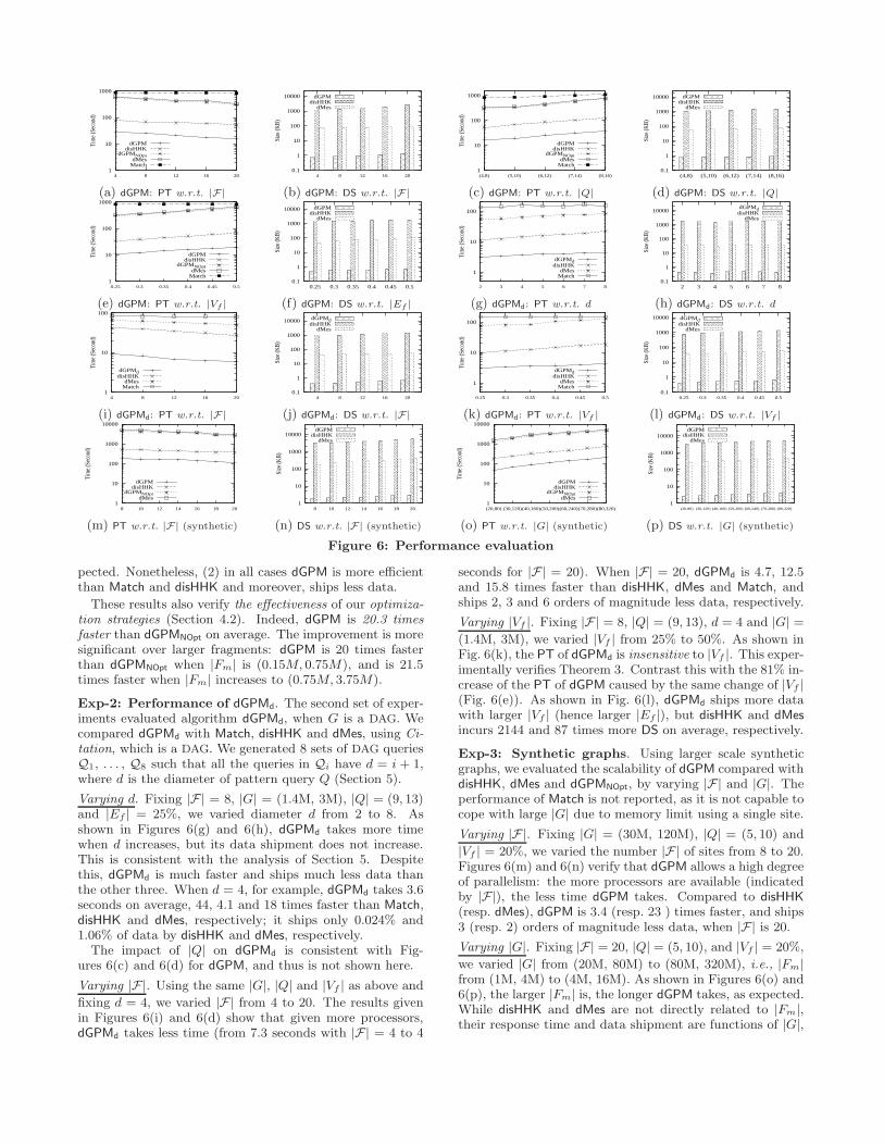
Exp-1: Performance of dGPM. We first evaluated theperformance of algorithm dGPM for general Q and G, com-pared with disHHK, Match, dMes and dGPMNOpt, using Ya-hoo. We identified 20 cyclic patterns with conditions suchas “domain = ‘.uk’ ”, and report the average here. We uselogarithmic scale for the y-axis in the figures for PT and DS.

Varying |F|. Fixing |G| = (3M, 15M), |Q| = (5, 10) and |Vf |

= 25%, we varied the number |F| of sites from 4 to 20. Fig-ures 6(a) and 6(b) report the PT and DS, respectively. Theresults verify that dGPM allows a high degree of parallelism:the more processors are available (i.e., the larger |F| is), theless time dGPM takes. In contrast, Match is indifferent to|F|. Compared to disHHK, dGPM is 3.5 times faster, andships 3 orders of magnitude less data, when |F| is 20. Theimprovement over disHHK is more significant when |F| in-creases: it is 2.8 times faster (resp. ships 0.07% of the databy disHHK) when |F| = 4, and 3.32 times faster when |F|= 16 (resp. ships 0.05% of data). On average, dGPM is 21.6times faster than dMes, while the latter ships 80 times moredata, since dMes incurs redundant message passing. Weobserved slightly increased DS as larger |F| induces slightlylarger |Vf | (resp. |Ef |), despite of the adjustment using [27].

Varying |Q|. Fixing |F| = 8, |G| = (3M, 15M) and |Vf | =

25%, we varied query size |Q| from (4, 8) to (8, 16). As shownin Figures 6(c) and 6(d), when |Q| gets larger, so do the re-sponse time of all these algorithms (the logarithmic scalemakes the increase of Match less obvious), and data ship-ment of all but Match, as expected. Compared to disHHK

and dMes, dGPM is 3.6 and 20 times faster, and ships atmost 0.044% and 1.5% of their DS, respectively, when |Q| =(8, 16). Moreover, the data shipment of dGPM is much lesssensitive to the change of |Q| than the other two.

Varying |Vf |. Fixing |F| = 8, |G| = (3M, 15M) and |Q| =

(5, 10), we varied |Vf | (resp. |Ef |) from 25% to 50%. Asshown in Figures 6(e) and 6(f), (1) when |Vf | (resp. |Ef |)increases, dGPM takes more time (from 11 to 19 sec-onds) and ships more data (from 0.54K to 0.97K), as ex-

1

10

100

1000

4 8 12 16 20

Tim

e (S

econ

d)

dGPMdisHHK

dGPMNOptdMes

Match

(a) dGPM: PT w.r.t. |F|

0.1

1

10

100

1000

10000

4 8 12 16 20

Size

(KB)

dGPMdisHHK

dMes

(b) dGPM: DS w.r.t. |F|

1

10

100

1000

(4,8) (5,10) (6,12) (7,14) (8,16)

Tim

e (S

econ

d)

dGPMdisHHK

dGPMNOptdMes

Match

(c) dGPM: PT w.r.t. |Q|

0.1

1

10

100

1000

10000

(4,8) (5,10) (6,12) (7,14) (8,16)

Size

(KB)

dGPMdisHHK

dMes

(d) dGPM: DS w.r.t. |Q|

1

10

100

1000

0.25 0.3 0.35 0.4 0.45 0.5

Tim

e (S

econ

d)

dGPMdisHHK

dGPMNOptdMes

Match

(e) dGPM: PT w.r.t. |Vf |

0.1

1

10

100

1000

10000

0.25 0.3 0.35 0.4 0.45 0.5

Size

(KB)

dGPMdisHHK

dMes

(f) dGPM: DS w.r.t. |Ef |

1

10

100

2 3 4 5 6 7 8

Tim

e (S

econ

d)

dGPMddisHHK

dMesMatch

(g) dGPMd: PT w.r.t. d

0.1

1

10

100

1000

10000

2 3 4 5 6 7 8

Size

(KB)

dGPMddisHHK

dMes

(h) dGPMd: DS w.r.t. d

1

10

100

4 8 12 16 20

Tim

e (S

econ

d)

dGPMddisHHK

dMesMatch

(i) dGPMd: PT w.r.t. |F|

0.1

1

10

100

1000

10000

4 8 12 16 20

Size

(KB)

dGPMddisHHK

dMes

(j) dGPMd: DS w.r.t. |F|

1

10

100

0.25 0.3 0.35 0.4 0.45 0.5

Tim

e (S

econ

d)

dGPMddisHHK

dMesMatch

(k) dGPMd: PT w.r.t. |Vf |

0.1

1

10

100

1000

10000

0.25 0.3 0.35 0.4 0.45 0.5

Size

(KB)

dGPMddisHHK

dMes

(l) dGPMd: DS w.r.t. |Vf |

1

10

100

1000

10000

8 10 12 14 16 18 20

Tim

e (S

econ

d)

dGPMdisHHK

dGPMNOptdMes

(m) PT w.r.t. |F| (synthetic)

1

10

100

1000

10000

8 10 12 14 16 18 20

Size

(KB)

dGPMdisHHK

dMes

(n) DS w.r.t. |F| (synthetic)

1

10

100

1000

10000

(20,80)(30,120)(40,160)(50,200)(60,240)(70,280)(80,320)

Tim

e (S

econ

d)

dGPMdisHHK

dGPMNOptdMes

(o) PT w.r.t. |G| (synthetic)

1

10

100

1000

10000

(20,80) (30,120)(40,160)(50,200)(60,240)(70,280)(80,320)

Size

(KB)

dGPMdisHHK

dMes

(p) DS w.r.t. |G| (synthetic)

Figure 6: Performance evaluation

pected. Nonetheless, (2) in all cases dGPM is more efficientthan Match and disHHK and moreover, ships less data.

These results also verify the effectiveness of our optimiza-tion strategies (Section 4.2). Indeed, dGPM is 20.3 timesfaster than dGPMNOpt on average. The improvement is moresignificant over larger fragments: dGPM is 20 times fasterthan dGPMNOpt when |Fm| is (0.15M, 0.75M), and is 21.5times faster when |Fm| increases to (0.75M, 3.75M).

Exp-2: Performance of dGPMd. The second set of exper-iments evaluated algorithm dGPMd, when G is a DAG. Wecompared dGPMd with Match, disHHK and dMes, using Ci-tation, which is a DAG. We generated 8 sets of DAG queriesQ1, . . . , Q8 such that all the queries in Qi have d = i + 1,where d is the diameter of pattern query Q (Section 5).

Varying d. Fixing |F| = 8, |G| = (1.4M, 3M), |Q| = (9, 13)and |Ef | = 25%, we varied diameter d from 2 to 8. Asshown in Figures 6(g) and 6(h), dGPMd takes more timewhen d increases, but its data shipment does not increase.This is consistent with the analysis of Section 5. Despitethis, dGPMd is much faster and ships much less data thanthe other three. When d = 4, for example, dGPMd takes 3.6seconds on average, 44, 4.1 and 18 times faster than Match,disHHK and dMes, respectively; it ships only 0.024% and1.06% of data by disHHK and dMes, respectively.

The impact of |Q| on dGPMd is consistent with Fig-ures 6(c) and 6(d) for dGPM, and thus is not shown here.

Varying |F|. Using the same |G|, |Q| and |Vf | as above and

fixing d = 4, we varied |F| from 4 to 20. The results givenin Figures 6(i) and 6(d) show that given more processors,dGPMd takes less time (from 7.3 seconds with |F| = 4 to 4

seconds for |F| = 20). When |F| = 20, dGPMd is 4.7, 12.5and 15.8 times faster than disHHK, dMes and Match, andships 2, 3 and 6 orders of magnitude less data, respectively.

Varying |Vf |. Fixing |F| = 8, |Q| = (9, 13), d = 4 and |G| =

(1.4M, 3M), we varied |Vf | from 25% to 50%. As shown inFig. 6(k), the PT of dGPMd is insensitive to |Vf |. This exper-imentally verifies Theorem 3. Contrast this with the 81% in-crease of the PT of dGPM caused by the same change of |Vf |(Fig. 6(e)). As shown in Fig. 6(l), dGPMd ships more datawith larger |Vf | (hence larger |Ef |), but disHHK and dMes

incurs 2144 and 87 times more DS on average, respectively.

Exp-3: Synthetic graphs. Using larger scale syntheticgraphs, we evaluated the scalability of dGPM compared withdisHHK, dMes and dGPMNOpt, by varying |F| and |G|. Theperformance of Match is not reported, as it is not capable tocope with large |G| due to memory limit using a single site.

Varying |F|. Fixing |G| = (30M, 120M), |Q| = (5, 10) and

|Vf | = 20%, we varied the number |F| of sites from 8 to 20.Figures 6(m) and 6(n) verify that dGPM allows a high degreeof parallelism: the more processors are available (indicatedby |F|), the less time dGPM takes. Compared to disHHK

(resp. dMes), dGPM is 3.4 (resp. 23 ) times faster, and ships3 (resp. 2) orders of magnitude less data, when |F| is 20.

Varying |G|. Fixing |F| = 20, |Q| = (5, 10), and |Vf | = 20%,

we varied |G| from (20M, 80M) to (80M, 320M), i.e., |Fm|from (1M, 4M) to (4M, 16M). As shown in Figures 6(o) and6(p), the larger |Fm| is, the longer dGPM takes, as expected.While disHHK and dMes are not directly related to |Fm|,their response time and data shipment are functions of |G|,

and increase when |G| gets larger. Observe that dGPM is24.7, 3.6 and 27.5 times faster than dGPMNOpt, disHHK anddMes. It ships at most 0.077% and 0.9% of data shippedby disHHK and dMes on average, respectively.

Summary. We find the following. (1) Our algorithms scalewell with large G: their response time and data shipmentare not a function of |G|. (2) They allows a high degreeof parallelism: their response time is significantly reducedwhen more processors are used. For example, dGPM istwice faster when |F| is increased from 4 to 20. Comparedto Match, disHHK and dMes, it is 55.4, 3.5 and 21.6 timesfaster, and ships 6, 3 and 2 orders of magnitude less data,respectively, when |F| = 20. The improvement over otheralgorithms is even bigger when more processors are used.(3) The algorithms are efficient, e.g., dGPM takes lessthan 21 seconds when |G| = (3M, 15M), |Q| = (5, 10) and|F| = 12, and ships only 0.94K data. When Q or G is aDAG, dGPMd is 15.8, 4.7 and 12.5 times faster than Match,disHHK and dMes on average, respectively, with ordersof magnitude less data shipment. (4) Our optimizationstrategies are effective, and make dGPM 20 times faster.

7. CONCLUSIONWe have studied what is doable and what is undoable

for distributed graph simulation. We have shown that itis impossible to find distributed simulation algorithms thatare parallel scalable in response time or data shipment.Nonetheless, we have shown that distributed simulationis partition bounded, by providing algorithms whose re-sponse time and data shipment are not a function in thesize of graph G. We have also verified, analytically andexperimentally, that our algorithms scale well with big G.

One topic for future work is to study parallel scalabil-ity and partition boundedness for other graph queries, e.g.,graph pattern matching with subgraph isomorphism [33] andstrong simulation [24]. Another topic is to give a full treat-ment of the model advocated in this work by combiningpartial evaluation and message passing, comparing themwith, e.g., MapReduce and GraphLab [22]. In addition,to effectively query real-life graphs, one wants to combinedistributed processing with, e.g., graph compression, view-based query processing and top-k query answering.

Acknowledgment. Fan and Wu are supported in partby 973 Programs 2014CB340302 and 2012CB316200, NSFC

61133002, Guangdong Innovative Research Team Program2011D005, Shenzhen Peacock Program 1105100030834361,and EPSRC EP/J015377/1.

8. REFERENCES[1] Amazon. http://aws.amazon.com/ec2/.[2] Facebook statistics.

http://www.facebook.com/press/info.php?statistics.[3] Full version. http://www.cs.ucsb.edu/∼yinghui/full.pdf.[4] Trinity. research.microsoft.com/en-us/projects/trinity/.[5] V. L. Anh and A. Kiss. Efficient processing regular queries

in shared-nothing parallel database systems using tree- andstructural indexes. In ADBIS Research Communic, 2007.

[6] S. Blom and S. Orzan. A distributed algorithm for strongbisimulation reduction of state spaces. STTT, 7(1), 2005.

[7] J. Brynielsson, J. Hogberg, L. Kaati, C. Martenson, andP. Svenson. Detecting social positions using simulation. InASONAM, 2010.

[8] A. Buluc and K. Madduri. Graph partitioning for scalabledistributed graph computations. In Graph Partitioning andGraph Clustering, pages 83–102, 2012.

[9] F. Chung, R. Graham, R. Bhagwan, S. Savage, and G. M.Voelker. Maximizing data locality in distributed systems.JCSS, 72(8):1309–1316, 2006.

[10] G. Cong, W. Fan, and A. Kementsietsidis. Distributedquery evaluation with performance guarantees. InSIGMOD, 2007.

[11] W. Fan, J. Li, S. Ma, N. Tang, Y. Wu, and Y. Wu. Graphpattern matching: From intractable to polynomial time.PVLDB, 3(1), 2010.

[12] W. Fan, X. Wang, and Y. Wu. Performance guarantees fordistributed reachability queries. PVLDB, 5(11), 2012.

[13] W. Fan, X. Wang, and Y. Wu. Incremental graph patternmatching. TODS, 38(3), 2013.

[14] A. Fard, M. U. Nisar, L. Ramaswamy, J. A. Miller, andM. Saltz. A distributed vertex-centric approach for patternmatching in massive graphs. In Big Data, 2013.

[15] S. Flesca, F. Furfaro, and A. Pugliese. A framework for thepartial evaluation of SPARQL queries. In SUM, 2008.

[16] J. C. Godskesen and S. Nanz. Mobility models andbehavioural equivalence for wireless networks. InCoordination Models and Languages, pages 106–122, 2009.

[17] A. Greenberg, J. Hamilton, D. A. Maltz, and P. Patel. Thecost of a cloud: research problems in data center networks.SIGCOMM Comput. Commun. Rev., 39, 2008.

[18] M. R. Henzinger, T. Henzinger, and P. Kopke. Computingsimulations on finite and infinite graphs. In FOCS, 1995.

[19] M. Jamali. A distributed method for trust-awarerecommendation in social networks. CoRR, 2010.

[20] R. Kumar, J. Novak, and A. Tomkins. Structure andevolution of online social networks. In KDD, 2006.

[21] J. Leskovec, A. Singh, and J. Kleinberg. Patterns ofinfluence in a recommendation network. In Advances inKnowledge Discovery and Data Mining, pages 380–389.2006.

[22] Y. Low, D. Bickson, J. Gonzalez, C. Guestrin, A. Kyrola,and J. Hellerstein. Distributed GraphLab: A framework formachine learning and data mining in the cloud. PVLDB,2012.

[23] J. J. Luczkovich, S. P. Borgatti, J. C. Johnson, and M. G.Everett. Defining and measuring trophic role similarity infood webs using regular equivalence. Journal of TheoreticalBiology, 220(3):303–321, 2003.

[24] S. Ma, Y. Cao, W. Fan, J. Huai, and T. Wo. Capturingtopology in graph pattern matching. PVLDB, 5(4), 2011.

[25] S. Ma, Y. Cao, J. Huai, and T. Wo. Distributed graphpattern matching. In WWW, pages 949–958, 2012.

[26] G. Malewicz, M. H. Austern, A. J. C. Bik, J. C. Dehnert,I. Horn, N. Leiser, and G. Czajkowski. Pregel: a system forlarge-scale graph processing. In SIGMOD, 2010.

[27] F. Rahimian, A. H. Payberah, S. Girdzijauskas, M. Jelasity,and S. Haridi. Ja-be-ja: A distributed algorithm forbalanced graph partitioning. Technical report, SwedishInstitute of Computer Science, 2013.

[28] M. Rowe and O. Group. Interlinking distributed socialgraphs. In WWW, 2009.

[29] M. Shoaran and A. Thomo. Fault-tolerant computation ofdistributed regular path queries. TCS, 410(1):62–77, 2009.

[30] D. Suciu. Distributed query evaluation on semistructureddata. TODS, 27(1):1–62, 2002.

[31] Y. Tao, W. Lin, and X. Xiao. Minimal MapReducealgorithms. SIGMOD, 2013.

[32] R. E. Tarjan. Depth-first search and linear graphalgorithms. SICOMP, 1(2):146–160, 1972.

[33] J. R. Ullmann. An algorithm for subgraph isomorphism.JACM, 23(1):31–42, 1976.

[34] V. Venkataramani et al. TAO: how facebook serves thesocial graph. In SIGMOD, 2012.

[35] D. P. Woodruff and Q. Zhang. When distributedcomputation is communication expensive. In DISC, 2013.

[36] K. Zeng, J. Yang, H. Wang, B. Shao, and Z. Wang. Adistributed graph engine for web scale rdf data. In VLDB,2013.