1

Moral Impossibility in the Petersburg

Paradox: A Literature Survey and

Experimental Evidence∗

Tibor Neugebauer

University of Luxembourg

Abstract: The Petersburg gamble constitutes an important paradox in the history of ideas. It has been thought-provoking and led to important developments in the natural and behavioral sciences. The proposed resolutions of the paradox have involved deep reflections about the human mind by some of the most celebrated scientists of the past three centuries. This paper describes the paradox, and focuses on the resolutions that have been advanced in the literature while alluding to the historical context. In particular, Bernoulli’s moral impossibility concept is revisited and discussed. The study contributes experimental data to the discussion of the paradox. The decision-making of subjects is in line with the notion of moral impossibility; in valuing the gamble, people neglect the events that occur only with small probability. The study elicits the size of the probability that experimental subjects seem to neglect when they formulate their willingness-to-pay for the Petersburg gamble. It is argued that this behavior is boundedly rational, as the individual level of moral impossibility can be interpreted as an individual aspiration level in the art of conjecturing.

Keywords: Petersburg gamble; experiment JEL-code: B3; C44; C9; D8; G1; N0

Author’s address: Université de Luxembourg Faculté de Droit, d’Economie et de Finance Campus Kirchberg, K2 4, rue Albert Borschette L-1246 Luxembourg +352466644-6285 (telephone); -6811 (fax) Tibor.Neugebauer@uni.lu

∗ I thank Stephan Lengsfeld, Francis Lagos, Juan Antonio Lacomba, Hikmet Arslanoğlu and Özgür Toparlak for their support in the data collection process and John Hey for revising and discussing the instructions. Helpful comments by Ottwin Becker, Michael Birnbaum, Jim Cox, Rachel and David Croson, Ernan Haruvy, John Hey, Guillaume Hollard, Astrid Hopfensitz, Rudolf Kerschbamer, Patrick Kinsch, Martin Kocher, Louis Levy-Garboua, Ulrich Schmidt, Klaus Schredelseker, Reinhard Selten, Matthias Sutter and seminar participants at LUISS, UC Fullerton, University of Innsbruck, University of Luxembourg, University I of Paris, University of Dallas, 2008 ESA meeting Tucson and the 2008 GEW-Tagung Mannheim are acknowledged. Part of this work was done during my research stay at LUISS in February 2007. I thank LUISS and especially John Hey for the hospitality received.

2

[Since] it is only rarely possible to obtain complete certainty that is complete in every respect,

necessity and use ordain that what is only morally certain be taken as absolutely certain. It

would be useful, accordingly, if definite limits for moral certainty were established by the

authority of the magistracy. For instance, it might be determined whether 99/100 of certainty

suffices or whether 999/1000 is required. Then a judge would not be able to favor one side, but

would have a reference point to keep in mind in pronouncing a judgment. (James Bernoulli 1713;

quoted from the commented translation 2006, p. 321)1

In the art of conjecturing (James Bernoulli 1713), i.e. the measuring of an event’s probability, the

applicability of probability theory to empirical data crucially hinges on the concept of moral

certainty. Something is morally certain if its probability comes so close to complete certainty that

the difference cannot be perceived. In contrast, something is morally impossible if it has only as

much probability as the morally certain falls short of complete certainty (Bernoulli 2006, p. 316).

Moral impossibility is thus defined as the subjective probability level which is negligibly small in

the conjecturing on the likely cases of events. Only by establishment of such a probability level

can we achieve the certainty that we need for scientific knowledge accumulation. Without

accepting such a probability level, conjecturing about the likely cases of events is only possible in

extreme cases since complete certainty cannot usually be attained through experimentation and

observation.

One historically important example of the games of chance in which moral certainty and

complete certainty lead to extremely different valuations is the so-called Petersburg paradox in

which a fair coin is repeatedly tossed until heads shows up for the first time. While a non-zero

probability exists that the coin is tossed forever, a fact that poses a non-finite mathematical

expected payoff for the gamble, the occurrence of an infinite run of tails is morally impossible.2 A

long finite run is also morally impossible, however, in a single trial of the gamble. Long

simulations in experimental statistics hardly ever report the occurrence of more than twenty

subsequent tosses. A run of twenty tails approximately corresponds to the odds of one in a

million. In the history of thought, it has been proposed that in a single trial of the Petersburg

gamble even a relatively small number of tosses can be considered as morally impossible. In this

paper, this proposition is experimentally tested through the elicitation of subjects’ willingness-to-

pay for various truncated versions of the Petersburg gamble that differ in the maximum payoff.

The experimental data show that all versions of the Petersburg gamble which allow for more than

six repeated tosses of tails elicit the same willingness-to-pay. From this evidence it is concluded

1 Throughout the paper the “Ars Conjectandi” of James Bernoulli (1713) is quoted by referring to Dudley Sylla’s English translation and commentary, “The Art of Conjecturing…,” which was published in 2006. 2 An even more striking example where moral impossibility is pitted against mathematical probability is the event that a monkey randomly hitting keys on a typewriter will write a given text, such as the Bible (Emile Borel 1914). Again, while this event has a mathematical probability greater than zero, it is morally impossible that it occurs. Or imagine the possibility that within a generation of mankind only boys and no girls are born or vice versa; although this event is more likely than an infinite run of tails when a fair coin is tossed repeatedly it is still morally impossible.

3

that subjects neglect those outcomes in the Petersburg gamble which occur with a probability

smaller than or equal to one in sixty-four.

Although the notion of moral impossibility is older than expected utility theory, it has

been largely neglected in economics and, in particular, in the modern discussion of the Petersburg

paradox. Expected utility has been the only standard solution to the Petersburg paradox in

economics textbooks. Nevertheless, the notion that there exists a smallest probability-unit of

interest for decision-making under uncertainty has applications to economics and the social

sciences far beyond the Petersburg gamble.3 In everyday life, people neglect cases whose events

they perceive as being unlikely. Ultimately the neglect of small probabilities might have increased

the likelihood of the occurrence of great disasters (Nassim Nicholas Taleb 2007; see also Klaus

Spremann 2008).4

The paper is organized as follows. The following section describes the Petersburg gamble

and alludes to the historical perspective.5 In addition to earlier surveys, the present paper

includes the experimental contributions to the Petersburg paradox (in section 3), highlights the

application of moral impossibility and uncovers interesting details that have been neglected in the

history of the paradox. These unnoticed details include, for instance, the tension between the

outcome of the law of large numbers and the theorem on infinite series which must have puzzled

the founder of the gamble, Nicholas Bernoulli, and which he proposed to resolve by invoking the

moral impossibility concept; the paradoxical risk preference that arises for a seller of the

Petersburg gamble; and the dilution concern that can arise when an institution offers the gamble

for sale. The review of the literature continues in section 2 with a focus on the solution concepts

3 Among other advantages, we obtain a well-defined unbounded utility function (Peter Wakker 1993). 4 A pamphlet by Coleen Rowley argues that the FBI had prior information about the terrorist attack of 9/11, and if the trace had been seriously followed up the attack could have been prevented (http://www.time.com/time/covers/1101020603/memo.html). Evidently, the risks of deteriorating real estate markets were neglected in what led to the subprime crisis (http://knowledge.wharton.upenn.edu/article.cfm?articleid=1998). In recent months, the collider experiment has started in Geneva. Doubts have been raised that, in the experiment, black holes can be generated that may subsume the world. These fears have been played down by specialists as ‘baloney’, although we have no experience with black holes and no mathematical proof has been provided that renders these fears invalid. John Huth, a professor of physics at Harvard, was cited (http://edition.cnn.com/2008/TECH/09/08/lhc.collider/) as saying that “the gravitational force is so weak that you'd have to wait many, many, many, many, many lifetimes of the universe before one of these things could [get] big enough to even get close to being a problem.” This statement could be taken as a confirmation that a terrible disaster can happen with a very, very, very, very, very small probability greater than zero. The world community seems to accept running this risk. 5 The Petersburg paradox has seen dedicated surveys by Emanuel Czuber (1882), Paul A. Samuelson (1977), Gérard Jorland (1983; 1987), Glenn Shaffer (1988), and Jacques Dutka (1988). The literature has been partly surveyed and historically discussed, furthermore, in Isaac Todhunter (1865), John Maynard Keynes (1921), Karl Menger (1934), George Stigler (1950), Kenneth Arrow (1952), Leonard Savage (1954), Otto Spiess (1975), Maurice Allais (1979), Gilbert Bassett (1987), and in Lorraine Daston (1988). Furthermore, the story is covered in many interdisciplinary books, including economics (e.g. Hans-Werner Sinn 1980; Klaus Schredelseker 2002), history of science (Peter Bernstein 1996), mathematics and statistics (Richard Epstein 1977; Warren Weaver 1982), philosophy (Richard Jeffrey 1983; Michael Resnik 1987; Ian Hacking 2001), sociology (Russell Hardin 1982), psychology (Scott Plous 1993) and appears on several Internet pages (e.g. http://www.wikipedia.org; http://plato.stanford.edu/archives/win1999/entries/paradox-stpetersburg/).

4

that constitute the testable hypotheses for the experiment, the results of which are detailed in

section 4. In line with the presented evidence, moral impossibility (i.e. the neglect of small

probabilities) seems to be the most convincing hypothesis. This conclusion is backed up with the

presentation of three experimental studies. The first study of the Petersburg gamble shows that

unlikely payoffs have no impact on subjects’ revealed willingness-to-pay as the same valuations

are elicited for different length of the gamble. The other two studies follow up on this result and

elicit the threshold level beyond which these valuations do not change. All gambles that involved

probability levels smaller than 1/16 and maximum payoffs greater than 16 Euro elicited the same

distribution of valuations. From this observation it is concluded that the small probabilities of

higher payoffs are neglected, assuming that the small amount of maximum payoff cannot

represent a level of maximum utility. Section 5 summarizes and discusses the results of the paper.

1 The birth of the problem

On September 9, 1713, so the story goes, Nicholas Bernoulli proposed the following problem in

the theory of games of chance, after 1768 known as the St Petersburg paradox (Sandor Csörgö

2001, p. 62), in a letter mailed from Basel to the mathematician Pierre Reymond de Montmort

(Daniel Bernoulli 1954, p. 33).6

Peter tosses a coin and continues to do so until it should land heads when it comes to the

ground. He agrees to give Paul one ducat if he gets heads on the very first throw, two

ducats if he gets it on the second, four if on the third, eight if on the fourth, and so on, so

that with each additional throw the number of ducats he must pay is doubled. Suppose we

seek to determine the value of Paul’s expectation.

The author of the problem, Nicholas Bernoulli (1687–1759), was the leading figure in stochastics

in the second decade of the eighteenth century (Csörgö 2001, p. 60; see also Anders Hald 1990).

In 1711, he provided a general solution to the most difficult problem in stochastics of that time,

the duration of play (Karl Kohli 1975), which was a generalization of Blaise Pascal’s (1623–1662)

6 The gamble received its name from the fact that the seminal paper of Daniel Bernoulli was presented and published in the journal of the Imperial Academy of Sciences in Saint Petersburg, which was founded by Catherine the Great in 1725. I have found a first reference to the Petersburg problem in the memoir 23 of Jean le Rond d’Alembert (1768, p. 78); in his contribution, d’Alembert refers first to the “problem in the memoirs of Petersburg” before he switches to the term “Petersburg problem” which he uses thereafter in all later contributions (see also Jorland 1987, p. 165).

The original problem by Nicholas Bernoulli involved the roll of the die (Montmort 1713, p. 402). The flip of the coin was introduced to the problem by Gabriel Cramer, who thus reformulated the problem of Nicholas Bernoulli into its definite form in a letter from London dated May 21, 1728 (see Spiess 1975). In the original proposal, Nicholas Bernoulli posted five problems to Montmort, of which the last two were predecessors of the Petersburg gamble (see equations (1) and (2) below). The fourth problem involved a lottery that paid one “ECU” for each roll of an ordinary die until six points were achieved for the first time, i.e. the lottery pays k + 1 if k is the number of rolls of the die before six points show up first. The fifth problem involved the power series of payoffs 2k, 3k, k2, and k3, substituting for k in the lottery of the fourth problem. The difference between the fourth and the fifth problem is that the fourth problem yields an expected payoff of six, while the expectations in problem 5 do not all exist.

5

problem of points and Huygens’s gambler’s ruin problem (see also Keith Devlin 2008). It should

be noted that the problem of the duration of play was introduced by Montmort (1708) and that it

is methodologically similar to the Petersburg gamble.7 Nicholas was the student and nephew of

the founder of probability theory, James Bernoulli, and wrote the foreword to the posthumously

published Ars Conjectandi, i.e. the unfinished masterpiece of his uncle, in 1713, which contained

the first proof of the law of large numbers.8 Nicholas also provided a proof of the law of large

numbers in a letter to Montmort where he indirectly introduced the normal distribution thus

preceding Abraham de Moivre (Oscar Sheynin 1970, p. 232). James, the most famous

representative of the whole Bernoulli had the great vision to provide, via the law of large numbers,

a justification for the measurement of empirical probabilities from observed frequencies. With

increasing sample size, he argued, one can learn from experiment, a posteriori (i.e. after the event

has happened), the hidden probabilities of cases in which an event can occur. Owing to his early

death, however, he could not finish the important fourth part of the Ars Conjectandi, whose title

indicates applications of probability theory to civil, moral and economic affairs but whose content

lacks such applications.9 Nicholas Bernoulli (1709) carried on this project and applied his uncle’s

theory to morals and the social sciences in his thesis De usu artis conjectandi in iure.10 He also

7 The problem of the duration of play, also known as the ruin problem (see below for the formulation of the problem of ruin by Maurice Allais 1979), may be formulated as follows: two players, Peter and Paul, are endowed with m and n ducats respectively. They repeatedly play a game in which Paul has probability of winning p and Peter has probability q = 1 – p. The winner in a game gets a ducat from the loser. The game is repeated until one of the players has lost all his ducats. What is the probability that the game ends at the kth gamble or before? Montmort (1708) solved this game for the special case of m = n = 3 and p = q = ½. 8 The law of large numbers shows that the sequence of independent Bernoulli trials converges to its expectation with an increasing number of observations. Before the name “the law of large numbers” was introduced to the literature by Simeon Dennis Poisson (1781–1840), it was called Bernoulli’s theorem (see Todhunter 1865). 9 James Bernoulli had already started working on his masterpiece twenty years before his death. From the reading of his scientific diary, Mediationes, one can conclude that the proof for the law of large numbers was written earlier, sometime during the years 1689 to 1692 (ibid., p.32). James said the delay in publication was because of his bad health and laziness at writing (ibid., p. 36). He also said that the most important part, the application to civil, moral and economic matters, was missing. Thus it has been suggested that he did not publish the book because he lacked both data and knowledge of economic issues to which he could apply his theory (ibid., p. 49). He asked Gottfried Wilhelm Leibniz (1646–1716) for both data (in the form of a book on life annuities by Jan de Witt (1675), a former student of René Descartes (1596–1650)) and proposals for applications, but did not receive either before his death (ibid., p. 49). As Nicholas Bernoulli writes in the foreword to the Ars Conjectandi, the publishers might have hoped that James’s brother, John (= Johann) Bernoulli (1667-1748), who was James’s successor to the chair of mathematics at Basel and the supervisor of Nicholas’s thesis after James’s death, would supply the missing part. Nicholas reiterates that they also tried to give the job to him, but he declined because he felt himself unequal to it (ibid., p. 129). While Nicholas wrote the foreword and supplied a page of errata to the publication, he was not the publisher of the Ars Conjectandi as has repeatedly been stated in the literature. As recent research showed, there has been historical confusion (possibly resulting from the entry to the Mathematisches Lexikon by Christian von Wolff in 1716), as the son of James, a painter named Nicholas “the younger” and born in the same year as Nicholas, took the book to the publisher (Bernoulli 2006, p. 60). 10 The title of his thesis translates into English as “the usage of the art of conjecturing in jurisprudence.” Nicholas submitted the thesis to the law faculty at Basel in 1709 to become a doctor of law. In the foreword to his thesis he acknowledges the great influence of his uncle’s unpublished

6

offered to supply the unfinished parts to the Ars Conjectandi (as he mentioned in a letter to

Leibniz) but, in the end, the family decided to publish the masterpiece “as is” in order to

underline James’s priority in the foundation of probability theory (Bernoulli 2006, p. 61). In the

foreword to his uncle’s masterpiece, Nicholas invites the reader and, namely, Montmort and de

Moivre, to apply the calculus of probabilities to morals, economics and politics.

According to the theory of the summation of infinite series, which we also owe to James

Bernoulli, one obtains the mathematical expectation of the Petersburg gamble by summing the

series of the probability weighted payoffs. Each product of probability and outcome in this series

yields one half; the first toss of the coin ends the game yielding one ducat with the probability one

half, the second toss of the coin ends the game yielding two ducats with a probability of one

quarter, etc. Let the expectation operator be denoted by E, and X is the random variable that

describes the possible outcomes; equation (1) gives Paul’s expectation.

∑=

∞→⎟⎠⎞

⎜⎝⎛×=+++=

n

i

ii

nXE

0 212

21lim...

84

42

21][ (1)

The series is divergent; it has no finite expectation (for a discussion see John Broome 1995). The

fact that the right hand side is infinite suggests a risk neutral gambler should be willing to pay any

fixed amount to purchase the right to play the gamble. The Petersburg gamble was the last of five

mathematical problems which Nicholas presented in the letter to Montmort. The preceding,

fourth, problem was identical to the fifth problem in terms of probabilities but involved a payoff

stream that increased by only one ducat per toss of the coin rather than by doubling the stakes on

each toss, as in equation (1). While the fourth problem allows also an unbounded payoff, the

payoff-probability products are converging, and therefore the expectation is finite, as

acknowledged in equation (2).

∑=

∞→=⎟

⎠⎞

⎜⎝⎛×=+++=

n

i

i

niXE

02

21lim...

83

42

21][ (2)

A comparison of the sums in (1) and (2) reveals that the payoff power function of i produces the

divergence of the expectation in the first equation. Nicholas Bernoulli stated that the discrepancy

between these problems was “most curious” (Montmort 1713, p. 402).11 With his expertise on

manuscript Ars Conjectandi on his choice of subject. In the thesis, he also addressed problems that were discussed in James’s scientific diary, Meditationes, which was not intended for publication. Before his thesis, Nicholas responded to his uncle’s work on the summation of infinite series in his defense for the master-of-arts degree in 1704 (Bernoulli 2006, p.55). He taught mathematics at the University of Padua between 1716 and 1719 where he worked on differential equations and geometry. At the University of Basel he became a professor of logics in 1722 and a professor of law in 1731. He corresponded with Montmort (1678-1719) and de Moivre (1667-1754) and also with Leibniz on converging and diverging series in 1712 and 1713 (Jacques Dutka 1988, p. 20). Biographies of Nicholas Bernoulli have been supplied by Joachim Otto Fleckenstein (1968), Kohli (1975), Adolphe Youschkevitch (1987), Hald (1990), Csörgö (2001), Norbert Meusnier (2006) and Bernoulli (2006). 11 It is imaginable that this remark and the eye-catching exposition of the problem may have had an influence on some of the historical solution proposals. For instance, Daniel Bernoulli (1738) proposed to sum the probability weighted logarithm of payoffs in (1) instead of the probability weighted payoffs (see the following section).

7

infinite series and the law of large number, the expectations in equations (1) and (2) must have

appeared extremely puzzling to Nicholas. On one hand, we have the approximation due to the

infinite series theorem; if a fair coin yields an infinite run of heads, the outcome exceeds any

bound in both problems. Yet, the probability weighted average is assumed to be a small finite

number in one case but infinite in the other. The question seems to be permitted if there are

degrees of infinity, and that is what Nicholas asked.12 On the other hand and implied by the law of

large numbers, if a fair coin is tossed infinitely often the relative frequency of heads and tails

must be the same with probability one. As a consequence, an infinite run of heads is impossible.

This obvious tension between the outcomes of the infinite series theorem and the law of large

numbers can be resolved in the theory of James Bernoulli by recurring to the moral impossibility

concept which also makes it possible to narrow the fair values of the two gambles (1) and (2)

whose intuitive values seem not to differ by much.

Montmort was not interested in the application of probability theory to morals and ethics

(Csörgö 2001, p. 61) and apparently did not contribute to the discussion of the problem.13 After

Montmort’s death, the young mathematician Gabriel Cramer proposed to Nicholas Bernoulli two

resolutions to the problem in 1728. In a letter which is reproduced in and appended to the paper

of Daniel Bernoulli (1954, p. 33), Cramer also states the paradox; according to the calculation,

Paul must give to Peter an “infinite sum” as an equivalent, “which seems absurd, since no person

of good sense, would wish to give 20 ducats.” Thus, the Petersburg paradox represented a

counter-example to Pascal’s wager. Pascal had argued and lived his adult life in accordance with

the theory that it is worth to abandon all riches for the small chance of winning an infinite

pleasure. The resolutions to the Petersburg paradox which have been presented in the literature,

including that of Cramer, are discussed in the following section.

2. Proposed resolutions of the paradox

There have been several proposals for the resolution of the Petersburg paradox in the literature

throughout the centuries. The most famous concept, expected utility theory, which has been the

standard approach referred to in economics textbooks, was proposed by Nicholas Bernoulli’s

cousin, Daniel Bernoulli. Daniel Bernoulli submitted a copy of his unpublished paper to Nicholas

Bernoulli on April 4, 1732, and it was published in 1738.

2.1 Expected utility14

12 In the original correspondence to Montmort (1713), Nicholas Bernoulli pointed out that the “expected infinite sum” (or even greater sum “if it is permitted”) cannot be the value of the lottery, “since it is morally impossible that [Paul] does not achieve [heads] in a finite number of throws” (Spiess 1975, p. 558). A translation to English of Spiess’s collection of Nicholas Bernoulli’s correspondences on the Petersburg gamble has been published by Pulskamp (1999). 13 At first, Montmort seemed uninterested in the problem. Later he promised to prepare a manuscript on the issue, which has never been found and to which no further reference was made in any known correspondence of Nicholas Bernoulli (Spiess 1975). Montmort died from smallpox in 1719. 14 Nicholas Bernoulli sent his problem set to Daniel Bernoulli, who was a professor of mathematics in Petersburg at that time. In his letter he indicated the paradox as pointed out by Gabriel Cramer and said that it was irrational to value the gamble above 20 ducats. Daniel Bernoulli replied to his cousin in November 1728 that the paradox is found in the small probability that the gamble will last for more

8

In Daniel Bernoulli’s expected utility theory, prospective wealth is weighted by the probability of

occurrence. The expected utility for the Petersburg gamble is the sum of the probability weighted

utility levels of wealth and thus depends also on the initial wealth α of the decision-maker.

∑=

∞→

+=+

++

++

+=+

n

ii

i

n

uuuuXEu0 2

)2(21lim...

8)4(

4)2(

2)1()( ααααα (3)

Equation (3) represents Paul’s expected utility from the Petersburg gamble in the general

formulation.15 Daniel Bernoulli used the logarithmic utility function, u(X) = log X. He argued

that, at the margin, utility of additional wealth is inversely proportional to the possessed wealth.16

A person whose wealth amounts to 100 ducats appreciates another cent approximately as much

as a person who has an initial wealth of 1,000 ducats appreciates another ten cents. In other

words, the marginal utility decreases in inverse proportion to the possessed wealth. The certainty

equivalent for the Petersburg gamble is therefore an increasing function of possessed wealth; the

opportunity of playing the Petersburg gamble would be worth two ducats if Paul possessed

nothing, about three ducats if his initial wealth were ten ducats, about four if his initial wealth

were 100 ducats, and about six if his initial wealth were 1,000 ducats.17 A very rich person would

have the certainty equivalent of 20 ducats (Bernoulli 1954, p. 32).

Gabriel Cramer had already suggested in 1728 that “men of good sense” value a prospect

by its “moral expectation” rather than by its “mathematical expectation” (Bernoulli 1954, p. 34).

He assumed, in a seemingly arbitrary manner, that the utility function takes the form of the

square root, as he argued that one may receive double the pleasure from 40 million than from 10

million. He computed the certainty equivalent without paying attention to initial wealth yielding

an approximate equivalent of 2.9. He can be credited with being the first to propose the idea of

diminishing marginal utility. His solution, however, did not take into account the initial wealth

than 20 or 30 throws, and in a follow-up letter a year and a half later he stated that a person would not wager an infinite sum when there was only an infinitesimally small probability of winning. Only in July 1731 did he compose a draft of his famous expected utility. There has been speculation that the draft benefited from discussions with his friend and colleague Leonhard Euler (1707-1783), who prepared but did not finish a paper on the same issue, (it was only published 79 years after Euler’s death) (Euler 1862; see also the discussion of Euler’s contribution by Ed Sandifer 2004). 15 The general formulation of expected utility is owed to John von Neumann and Oscar Morgenstern (1947), who established the axiomatic approach (in this they were anticipated, however, by Frank Ramsey 1931). The standard term “expected utility” is a modern translation of the term “emolumentum medium” used by Daniel Bernoulli (1738). In the Econometrica translation of Bernoulli’s article, the term “moral expectation” or “mean utility” is used (see Bernoulli 1954, p. 24, footnote 3). The term “moral expectation” or “moral value”, however, was introduced by Gabriel Cramer (1728), when he discussed the Petersburg gamble. The term was later used by Pierre-Simon Laplace (1820). 16 For human perceptions of just noticeable differences, the psychophysical “Weber-Fechner” law suggests a logarithmic relationship between stimulus and perception (for a survey see Duncan Luce and Patrick Suppes 2002). 17 The certainty equivalent is the amount to pay that makes you indifferent whether you purchase the gamble or not. For a person with initial zero wealth and a logarithmic utility function, Daniel Bernoulli (1954) computed the expected utility, of log 2, and the certainty equivalent, of 2 ducats, as the inverse utility function.

9

position and thus Bernoulli’s solution must be considered as superior in both sophistication and

reason.18 Laplace (1820) accepted the idea of diminishing marginal utility and called it the tenth

principle of probability. He showed that mathematical expectation was the limit of moral

expectation when the division of risks becomes infinite and thus used it as the foundation for his

theory of insurance (Jorland 1987, p. 171).

During the following two hundred years, Daniel Bernoulli’s utility theory was discussed,

appreciated for the possibility it gave of making interpersonal comparisons (Knut Wicksell 1900),

and generalized. Francis Edgeworth (1881) rejected the logarithmic utility function for being as

arbitrary as any other concave function, Alfred Marshall (1890) replaced the wealth argument in

the function by income, Vilfredo Pareto (1893) replaced it by consumption, and Max Weber

(1908) suggested that the utility function can vary for one good or another. Karl Menger (1934),

finally, showed that utility must be bounded from above. He based his argument on the

Petersburg gamble. Given Bernoulli’s logarithmic utility function, the paradox is reinstated by

replacing the power-series 2i in equation (1) by the exponentially increasing power series i

e2

since this payoffs series yields a non-finite expected utility and thus a non-finite certainty

equivalent. Since a corresponding super-power series can be found for every unbounded utility

function (Menger 1934, p. 468f), the only way to circumvent the paradox in the expected utility

framework requires a cut-off level for utility where any further increase in payoff leaves the

decision-maker at the same utility level. Such a cut-off level to utility was also suggested by

Gabriel Cramer in 1728. He argued that the sum of 2100 or 21,000 ducats would give him no more

pleasure and attract him more to accept the gamble than a payoff of 224 (≈ 16 million) ducats; a

maximum payoff of sixteen million gives an expected payoff of thirteen ducats. Motivated by

Menger’s discussion, von Neumann and Morgenstern (1947) introduced the axiomatic approach

to expected utility in the second edition of their “Theory of Games and Economic Behavior” (see

Menger 1967, p. 211). Kenneth Arrow (1971) showed that to avoid the super-Petersburg paradox

and for a complete ordering of all probabilistic outcomes, the utility function must be bounded

from both above and below (see also Stigler 1950; Savage 1954; D.L. Brito 1976; Robert Aumann

1977). The double-sided boundedness and other important properties of the utility function to

avoid the super-Petersburg gamble are also discussed in Samuelson (1977).

While mathematically boundedness is a necessary condition for the utility function to be

well-defined, the flat utility function beyond a certain wealth as proposed by Gabriel Cramer

seems to misrepresent human behavior. Although people might feel indifferent between a payoff

of 2n and 2n+1 for n ≥ 24 or an arbitrary integer, as Cramer suggested, it is doubtful that people

would choose 2n over 2n+1 when facing the choice. Even if the decision-maker does not choose the

18 George-Louis Leclerc Buffon (1707–1788), who learnt the Petersburg gamble from Cramer on a trip to Geneva in 1731 (Yves Ducel and Thierry Martin 2001), contributed several approaches to a resolution of the paradox which he published in his famous essay (Buffon 1777). His first solution involved diminishing marginal utility, which he communicated to Cramer on October 3 1730, that is, prior to Daniel Bernoulli’s publication (Buffon 1777, p. 75ff). Buffon’s utility took the initial wealth position of Paul as a point of reference and weighted losses more than gains (see also below).

10

double amount for their own wellbeing, the double amount would simply be chosen for the sake

of passing on their advantage to the children and all children’s children. More generally speaking,

a bound on utility seems to stand in contradiction to the observed competitive nature of the

human race, the conqueror of the earth and of our sun system. There should be no doubt that

humans prefer governing the entire universe to governing the universe except for the earth. The

Petersburg gamble is ultimately a gamble on the earth and the universe.

2.2 Moral impossibility and moral certainty

In reaction to the proposal for using the expected utility approach to the resolution of the

Petersburg paradox, Nicholas Bernoulli (1732) replied to his cousin on April 5, 1732:

I have read [your manuscript] with pleasure, and I have found your theory most

ingenious, but permit me to say to you that it does not solve the knot of the problem in

question. There is not agreed to measure the use or the pleasure that one derives from a

sum that one wins, nor the lack of use or the sorrow that one has by the loss of a sum;

there is agreed no longer to seek an equivalent between the things there; but there is

agreed to find how a player is obliged in justice or in equity to give to another for the

advantage that therein accords him in the game of chance in question, or in other games

in general, so that the game is able to be deemed fair, as for example a game is considered

fair, when the two players bet an equal sum on a game under equal conditions, although in

your theory, and in paying attention to their wealth, the pleasure or the advantage of gain

in the favorable case is not equal to the sorrow or the disadvantage that one suffers in the

contrary case.19 Mr. Cramer has also tried to resolve the problem by reflecting on use or on

pleasure that men are able to derive from money, but without paying attention to the sum

of goods that one already possesses. Here is that which he has written to me in 1728 on

this matter: (It follows a quote of the letter of Gabriel Cramer 1728.) I have indicated to

him next that it would seem to me that in admitting this assumption, that a man of good

sense is not willing to give 20 ducats, because he estimates all the cases which give him a

lesser sum than 20 ducats possible, and each of the others, which are able to give a greater

sum, impossible; that in admitting, I say, this assumption, one is able to evaluate his

expectation

212...032016

3218

1614

812

411

21

=++⋅+⋅+⋅+⋅+⋅+⋅ (4)

I claim that this reasoning is not too exact, but I believe that in matching together your

idea and that of Mr. Cramer and my own on that it is necessary to estimate a small

19 Note that Nicholas’ notion of a fair gamble requires Peter and Paul to be indifferent, while Daniel’s solution assigns a fair value of the gamble only to Paul.

11

probability as null, one is able to determine exactly the sought equivalent [for the

Petersburg gamble].20 (Spiess 1975, p. 566f, emphasis added)

This quote is an excerpt from Nicholas Bernoulli’s last preserved letter on the Petersburg gamble.

The knot in question is the moral impossibility of obtaining more than 20 ducats as a payoff in

the Petersburg gamble since the likelihood of such an event is too small; in his letter to Gabriel

Cramer he is more exhaustive on this issue.21 As stated above, the term moral impossibility was

introduced before by his uncle James in the Ars Conjectandi. It was defined as the reciprocal of

moral certainty.22 Moral certainty is one of the key concepts in James Bernoulli’s art of

20 Daniel Bernoulli (1954, p. 33) referred to the letter of his cousin in his famous article. “In a letter to me …, [Nicholas Bernoulli] declared that he was in no way dissatisfied with my proposition on the evaluation of risky propositions when applied to the case of a man who is to evaluate his own prospects. However, he thinks that the case is different if a third person, somewhat in the position of a judge, is to evaluate the prospects of any participant in a game in accord with equity and justice.” 21 Nicholas Bernoulli replied to Gabriel Cramer on July 3, 1728 (Spiess 1975, p. 562f):

The response that you give for the solution of the singular case proposed to Mr de Montmort page 402, Prob. 5 satisfies only part of it; it suffices, as you say, to make see that [Paul] must not give to [Peter] an infinite equivalent; but it does not demonstrate the true reason for the difference that there is between the mathematical expectation and vulgar estimate; for example in the case of Heads and Tails there is no person of good sense who wished to give 20 ECU, not for this reason that the use or the pleasure that one is able to draw from an infinite sum is barely greater than the one which can be taken of a sum of 10, or 20, or 100 millions, but because in giving for example 20 ECU one has a very small probability to win something, and that one believes the loss morally certain. The vulgar neither stakes here in the storyline nor of millions, nor of hundreds of ECU paying no attention at all to this that the terms of the geometric progression 1, 2, 4, 8, 16, etc. becoming fairly great they are able to be considered equal, he is enlisted through this neither to accept nor to refuse the game, it is determined solely by the degree of probability that he has to win or lose; to him a very small probability to win a great sum does not counterbalance a very great probability to lose a small sum, he regards the event of the first case as impossible, and the event of the second as certain. It is necessary therefore, in order to settle the equivalent justly, to determine as far as where the quantity of one probability must diminish, so that it be able to be deemed null; but here is that which is impossible to determine, any assumption that one makes, one encounters always difficulties; the limits of these small probabilities are not precise, but they have a certain latitude what one is not able to fix easily; a probability which for example has 1/100 certitude must not be reputed null instead that which has 1/99 certitude. It seems to me therefore in admitting this assumption that a man of good sense is not willing to give 20 ECU, because he holds for certain that the sum which will fall to him will be less than 20 ECU, one is able to find the equivalent sought by the following reasoning: by hypothesis it is morally impossible that he obtains 20 ECU; it will be therefore also morally impossible that he obtains 32 ECU or some other number of ECU in this progression 32, 64, 128, etc. ; or the probability to obtain a number of this progression is 1/64 + 1/128 + 1/256 + … = 1/32, therefore this man of good sense reputes a probability which does not surpass as null, and a probability which has as a total certitude, consequently his expectation will be worth by the rule 1/2 ⋅ 1 + 1/4 ⋅ 2 +…+ 1/32 ⋅ 16 + 0 ⋅ 32 + 0 +… = 2.5. [The original reads … 1/16 ⋅ 8 + 0 ⋅ 16 + … = 2, but is corrected in the later letter sent to Daniel Bernoulli]. But I do not know if this other reasoning will be more just: A man who does not want to give more than 20 ECU estimates all the cases which give to him a lesser sum than 20 ECU possible, and each of the others, which are able to give a greater sum, impossible; he regards therefore only the probabilities less than 1/32 as null, consequently his expectation will be worth 1/2 ⋅ 1 + 1/4 ⋅ 2 +…+ 1/32 ⋅ 16 + 0 ⋅ 32 + 0 +… = 2.5 [The original reads = 2]. There will be well again some things to say on this matter, but not having the leisure to arrange in order or to develop the ideas which are presented to my spirit, I pass over them in silence.

22 According to James Bernoulli’s definition, “the morally certain is that whose probability is almost equal to complete certainty so that the difference is insensible” (Bernoulli 2006, p. 316). Moral

12

conjecturing. According to the law of large number the likelihood increases that the observed

relative frequency falls inside a given neighborhood of the true probability with an increasing

number of independent observations. However, complete convergence is only attained in the limit

where the number of repetitions increases beyond any bound. To base a conclusion on a finite

number of observations we must discard outliers that occur with small probabilities by defining a

minimum probability level, i.e. the level of moral impossibility beyond which small probability

events can be treated as zero. Indeed a certain degree of subjective arbitrariness may be

unavoidable when we fix the aspiration level of moral impossibility. Therefore, James proposed

that the level of moral certainty or its counterpart moral impossibility must be established by the

judge according to the circumstances, whether 99/100 of moral certainty is sufficient or whether

999/1,000 is needed (Bernoulli 2006, p. 321). Given the level of moral certainty, he continued,

one can determine a posteriori (i.e. empirically) what we cannot derive a priori (i.e. the real

odds) by extracting it from a repeated observation of the results of similar examples. Only by

fixing a level of moral certainty can we make a judgment on the odds of the events of cases. A level

of moral impossibility is necessary for the advancement of knowledge in the natural sciences

under uncertainty. To determine empirical probabilities, James Bernoulli who also was a

professor of experimental physics proposed experiments such as the ones that had been reported

earlier by Antoine Arnauld and Pierre Nicole (1662) in the “Art of Thinking”; he said that “… this

empirical method of determining the number of cases by experiment is not new or

uncommon,”(Bernoulli 2006, p. 328). The Ars Conjectandi abruptly finishes after James

computes, for his first and only urn example, the required number of n > 25,500 experiments at a

certainty level of 1/1,000.23 It has been argued that this number might have appeared

disappointingly large to James Bernoulli, as his home town of Basel numbered fewer inhabitants

in those days. Given that Bernoulli was interested in applying probability theory to civil problems

such a large number posed a practical data collection problem. Stephen Stigler (1986, p. 77)

certainty has been introduced by Jean Charlier de Gerson (1363–1429), chancellor of the University of Paris around 1400. It is said that the concept goes back to a statement in Aristotle's Nicomachean Ethics “that one must be content with the kind of certainty appropriate to different subject matters, so that in practical decisions one cannot expect the certainty of mathematics.” Descartes put it in circulation; he describes “morally certain” as having sufficient certainty for application to ordinary life “(those who have never been in Rome have no doubt that it is a town in Italy, even though it could be the case that everyone who has told them this has been deceiving them)” (Rene Descartes 1985, p. 290). Moral certainty has had its relevance in jurisprudence, where it means beyond any reasonable doubt (this is the highest level of proof which is used mainly in criminal trials). Leibniz discussed moral certainty and degrees of probability in jurisprudence and introduced impossibility and possibility as events with zero and unity probability in 1665 (Keynes 1921, p. 155). In 1699, John Craig discussed levels of certainty in his theologiae christianae principia mathematica, a book Nicholas Bernoulli cited in his thesis when discussing witnesses and degrees of certainty. When Gabriel Cramer lectured on logics in about 1745, he discussed moral certainty and moral impossibility in line with the Ars Conjectandi and the Usu Artis Conjectandi in Iure (Thierry Martin 2006). 23 Actually, this number is larger than the required number owing to two crude approximations in James Bernoulli’s proof; Hald (2007, p. 14) reports n > 12,243.

13

suggested that Bernoulli quitted his work in frustration when he saw the huge number.24 One way

of revising the required number of observations to a smaller, more available sample size would be,

in fact, to lower the aspiration level on moral impossibility. Nicholas Bernoulli believed that the

Petersburg gamble requires the application of the moral impossibility concept to make it fair.25 It

is conceivable that he hoped to obtain a consent level of moral impossibility for the application in

the games of chance. In letters to Cramer and Daniel Bernoulli, Nicholas suggested that 1/64 and

smaller probability levels should be treated as zero. Other authors proposed different levels of

moral impossibility in the Petersburg gamble. D’Alembert (1764, p. 7) suggested that one would

not want to risk a fair amount of money on outcomes that occur with such a small probability of

1/128 or less, even if the potential earnings were immense. More recently and without further

justification or reference, Samuel Gorovitz (1979) proposed that the probability of 1/128 was

negligible in the Petersburg gamble.

Buffon (1777), who provided several proposals for the resolution of the Petersburg gamble,

argued that a probability smaller or equal to 1/10,000 generally cannot be distinguished from a

zero probability. In his days, the odds that a 56-year-old man would die in the course of a day

were 1: 10,180. He claimed that such a small probability is nothing to be worried about. Daniel

Bernoulli approved the idea of negligible probabilities in a letter to Buffon dated March 19, 1762

but demanded the application of the more conservative level of one in 100,000 (1777, p. 75); that

was also the probability level in physics that Huygens regarded as being equivalent to a

mathematical proof (Dutka 1988, p. 33). As the expected intensity of the fear of death in the

course of the day disappears if its likelihood is smaller than 1/10,000, and as this fear is much

greater than the intensity of all other sentiments such as fear or hope, Buffon (p. 90) believed that

a moral impossibility level of 1/1,000 should be applied to the estimate of the moral value of

money. He suggested that all payoffs of the Petersburg gamble that occur with a probability of less

than 1/1,024 can be regarded as almost zero, so that they are irrelevant for decision-making.

Buffon (1777) underlined this claim by experimental data. He conducted the first recorded

experiment in statistics to determine empirically the likely outcomes in the Petersburg gamble. A

child played out n = 211 = 2,048 trials of the Petersburg gamble (Buffon 1777, p. 48f). The reported

gamble outcomes are reproduced in the table A1 of the appendix. All trials ended after at least

24 James Bernoulli searched over 20 years for questions to which he could address the art of conjecture. He eventually learned about the existence of de Witt’s work on life rents including mortality tables (the work is printed in Kohli 1975b) and repeatedly called for its submission to him by Leibniz. From the correspondence with Leibniz it is evident that James Bernoulli was desperately searching for data to apply his theory. It is also possible that he left the application of his theory unwritten, since he never received the copy of de Witt’s book from Leibniz. 25 Nicholas referred to moral certainty in his reply to Montmort in 1713 (Spiess 1975, p. 558), when he motivated his fifth problem whose reformulation became later known as the St Petersburg paradox. Nicholas Bernoulli (1709) also acknowledged the relevance of moral certainty in the foreword to his thesis; “the art of conjecturing concerns uncertain and doubtful matters, about which, although complete certainty is impossible, we can nevertheless by conjectures define how great the probability is that this or that will be, what probably will happen, which outcome is more probable than another, or how much this or that conclusion diverges from complete certainty” (Bernoulli 2006, p. 55).

14

nine tosses and the average payoff was 4.9 ducats. Buffon concluded that about five ducats should

be a fair entry fee to the gamble. August de Morgan (1912) reported replications of Buffon’s

experiment by three anonymous correspondents and Dutka (1988) ran eleven Buffon experiments

on the computer. These fourteen Buffon experiments generated an average payoff of 7.3 ducats

per Petersburg gamble (Dutka 1988, p.35ff). David Tolman and James Foster (1981) ran 1,000

Buffon experiments with the computer generating an average payoff of 9.8 and a median average

of 6.8 ducats. Allan Cesar (1984), who varied the number of trials, n, from 100 to 20,000

repetitions, confirmed the theoretical result implied by the law of large numbers (see the section

below), in that an increase in repetitions leads to an increase of the average payoff, since longer

series make higher payoffs more likely. Manuel Russon and SJ Chang (1992) reported

inconsistencies of their data with this theory as they found that long runs (involving more than 20

tails) did not occur in computer trials. Contrary to this observation, Robert Vivian (2004)

reported evidence that was consistent with the theory. In summary, the results in the literature

are mixed. The longest run ever reported involved 28 tails (Ludger Hinners-Tobrägel 2003).26

Following up on the discussion of Buffon, d’Alembert (1761) raised the question whether

some unlikely events, e.g. 100 successive tosses of tails, can occur at all. He concluded that some

probability levels are simply too small to be physically relevant; some cases he claimed are purely

metaphysically possible and physically impossible.27 The idea of physical impossibility was most

prominently represented later by Auguste Cournot (1843).28 Cournot (p. 78) stated that it is

mathematically possible that a heavy cone stands in balance on its vertex, but it is physically

impossible as the probability of that event is vanishingly small. Similarly, he suggested that in a

long sequence of trials it is physically impossible for the frequency of an event to differ

substantially from the event’s probability (1843, p. 121 f). From these statements, the so-called

“Cournot’s lemma” has been introduced into the literature (Fréchet 1948; Glenn Shafer 2006).

26 Lola Lopes (1981) ran 100 simulations (representing businesses) with one million Petersburg gambles (representing buyers) for four different entry fees. A business would stay afloat as long as its balance sheet after fees and prize allocations remained above -$10.000, but it would close down otherwise. The study does not reveal the longest run of tails as Lopes focused on the survival of businesses. With a $25 fee only nineteen businesses stayed open after one million buyers; with a $100 fee, 90 businesses stayed open and the average gain was $55.9 million. 27 Similarly to Buffon (1707- 1788), d’Alembert (1717- 1783) contributed several essays to the study of the Petersburg gamble. In one essay, he argued that a run of 100 tails in a row may be metaphysically possible but it is physically impossible; suggesting that there are limits to the application of mathematics to the real world. In memoir 27, d’Alembert (1768, p. 299) states the following; given “2100 players who cast each one hundred times in sequence a similar piece into the air; I say that one can wager without any risk that any of these players will bring forth neither heads nor tails one hundred times in sequence”(quoted from the translation by Pulskamp 2004). 28 For the Petersburg gamble, Cournot (1843, p. 109) suggested a market solution. He proposed to sell lottery tickets which yielded a non-zero payout for one particular sequence of tosses only. He claimed that there would be one critical length beyond which every ticket would remain unsold and cited empirical evidence. In the French lottery, the administration had taken out a prize which occurred with a probability of one in 44 million, because it was too seldom gambled on. Cournot (1843, p. 106) said that “one imagines well that there must be a limit to the smallness of chance” (see also Jorland 1987, p. 182).

15

The principle states in its weak and strong forms that a small probability event will happen rarely

on repeated trials and it will not happen at all in a particular trial, respectively. Cournot’s lemma

has been viewed as the fundamental law which links probability theory to the real world by many

famous theoreticians, including Paul Levy (1925), Andrei Markov (1900), Andrei Kolmogorov

(1933) and, most drastically, Borel (for a survey see Glenn Shafer 2006). Borel (1939, p. 6f) called

the principle that an event with very small probability will not occur at any time “the single law of

chance”. He distinguished impossible events by measure; impossibility on the human scale: p <

10−6; impossibility on the terrestrial scale: p < 10−15; and impossibility on the cosmic scale: p <

10−50. Earlier, in 1930, he stated that probabilities below 10-1,000 can be universally neglected.

Borel rejected atomless probabilities as irrelevant for science, since one must be satisfied with five

or six decimal places for many experimental problems. The nondenumerable continuum, he

argued, is a purely metaphysical conception which has been useful as an approximation, but

denumerable sets are the sole reality we are capable of attaining (Borel 1909; Eberhard Knobloch

1987). Wakker (1993) also showed that denumerable probability permits an unbounded, but well-

defined, utility function.

It may be physically impossible to prove or disprove Cournot’s lemma by statistical

experiment, but it may be no wonder that the notion of physical impossibility has not been

generally accepted in the literature, as it lacks the additivity property. For instance, Nicolas de

Condorcet (1785), a former student of d’Alembert, took issue with treating small probabilities

equal to zero. Bruno de Finetti (1951) rejected the empirical irrelevance of small probability

events, although he tolerated the idea of neglecting small probabilities as a decision criterion

under uncertainty. In the nineteen-sixties, Cournot’s lemma disappeared from the literature in

favor of subjective probabilities and other theories (Shafer 2006, p. 11f). In the recent literature, it

has been pointed out that small probability events may have an extremely high impact on markets

since they are not sufficiently anticipated by the market participants (Taleb 2007). This

observation also seems to suggest that small probability events are neglected in the psychology of

decision-making until evidence shows up.

While both physical impossibility and moral impossibility lead to a finite expectation for

the Petersburg gamble, physical impossibility as suggested by the so-called Cournot’s lemma is a

much stronger statement than James Bernoulli’s moral impossibility. In contrast with the concept

of physical impossibility, the concept of moral impossibility does allow small probability events to

happen but regards it as unreasonable that they will occur, i.e. too unlikely to deserve

consideration. For matters of forensic judgment or scientific knowledge accumulation, a level of

moral impossibility must be established as a decision criterion. In jurisprudence, fingerprints,

blood or DNA are used as evidence beyond reasonable doubt, since it is statistically almost

impossible to find two identical fingerprints, blood groups or DNA.29 The likelihood is so small (<

29 In jurisprudence, three levels of certainty, so-called standard of proofs, are distinguished; preponderance of evidence (low level of proof), clear and convincing evidence (medium) and beyond a reasonable doubt (highest level) (for a detailed, historical exposition see Barbara Shapiro 1991). Depending whether the approach of elicitation was indirect or direct, evidence from surveys and

16

1/100,000) that it is taken as a proof of the offender’s identification (Patrick Kinsch 2008). In line

with James Bernoulli’s art of conjecturing, research in the natural sciences hardly ever employs a

moral impossibility level beyond one in a thousand. For the social sciences, Ronald Fisher (1925,

p. 102) suggested that a 5 percent level of significance is sufficient as a decision rule, since that

level includes approximately two standard deviations of the distribution and excludes only very

extreme outliers. The significance level represents an aspiration level of the decision-maker in

situations of risk and uncertainty. Fixing such a level is thus a boundedly rational approach

(Reinhard Selten 2001) in the art of conjecturing; depending on the individual aspiration level

and the severity, whether the possibility is concerned with suffering a fatal accident or the

possibility of finding a dollar on the pavement, this level of moral impossibility may largely vary.

Taking the frequently applied 5 percent level of significance as a level of moral

impossibility implies for our problem of repeatedly flipping a coin that all Petersburg-gamble

lengths which involve more than five tosses of tails on a single trial must be rejected as

unreasonable outcomes (an implication in line with Nicholas Bernoulli’s proposal). This result

would be implied by the null hypothesis of a fair coin that yields heads and tails with the same

probability. The distribution of possible runs under the null hypothesis is described by a

geometrical distribution with p = ½. Buffon (1777, p. 88f) made predictions of the experimental

outcomes according to this distribution; see table A1 in the appendix and the section 2.5 on the

“law of large numbers”.30 If all our evidence, i.e. the first trial, involves a longer run than five tails

we have to reject the null hypothesis in favor of the alternative of a biased coin which favors tails

more than heads. Laplace (1821) made a related argument; he suggested that if one tosses a coin

for which one side may be more likely than the other, you should rather bet on the more

frequently observed outcome if you do not know which side is more likely to land.

2.3 The law of small numbers and probability weighting

The opposite behavior to the rule of favoring the most frequent observation in repeated trials has

been reported from studies on probability matching and gambling. Ward Edwards (1961)

observed that subjects who imagined a coin-tossing experiment recorded shorter runs of heads

and tails than could be observed in a physical coin-tossing experiment.31 According to Daniel

experiments has shown that the individual equivalent for the highest level of proof lies somewhere between 70% and 90% of certainty (these results are surveyed in Reid Hastie 1993, 101-107). Jeremy Bentham (1843) discussed moral and physical improbability and impossibility in his treatise on the rationale of judicial evidence. 30 According to Buffon’s expectation heuristic, half of the gambles are expected to finish at the first toss, a quarter at the second toss of the coin, etc. After 211 - 1 expected outcomes assigned in that way, the last gamble outcome “can be ignored without error sensitivity” (p. 89), and is placed at the peak of the table. The thus expected payoff sum is 11,265 yielding 5.5 ducats as a fair value of a single Petersburg gamble. As his observed outcome of 4.9 ducats falls in the interval of 1/11 around this prediction, he claims his theory has been empirically supported. In the same way he predicts an average payoff of 0.5 x for n = 2x gambles. This result coincides with the limit distribution of William Feller (1945). 31 In repeated prediction experiments, subjects predict random events by picking outcomes in proportion to the frequency with which they expect the corresponding signal instead of picking the

17

Kahneman and Amnon Tversky (1971), people seem to believe that even a small sample should

represent the probabilities of the distribution from which it is drawn. This stylized fact has been

coined the “representative heuristic” or the “law of small numbers”.32 After observing one of two

independent outcomes, subjects are more likely to guess the other outcome since they expect the

relative frequencies to regress to the mean (Shefrin 2002). The belief in negatively correlated

chance events has been called the “gambler’s fallacy” (Matthew Rabin 2002; James Sundali and

Rachel Croson 2006).

The idea of such a regression to the mean was first expressed by d’Alembert (1780) in the

discussion of the Petersburg gamble. He pretended that after tails has landed twice heads

becomes more likely than tails.33 More rigorously, he proposed that if tails has arrived at the first

toss, the chance that heads arrives at the next is (1+ ε1)/2, and not ½; if tails has arrived at the

first two tosses, the chance that heads arrives at the next toss is (1+ ε1+ ε2)/2, and not ½; and so

on. The quantities εn are supposed to be small positive quantities, and subject to the limitation

that their sum is less than unity, and that the chance of tails is positive on each toss. On this

supposition, the fair price for the Petersburg gamble is a finite sum, i.e. half of the following series

(see Todhunter 1865, p. 288).34

1 + (1+ ε1) + (1 – ε1) (1 + ε1 + ε2) + (1 – ε1) (1 – ε1 – ε2) (1 + ε1 + ε2 + ε3) (5) + …

Without referring to d’Alembert, Menger (1934, p. 478) also suggested an underweighting

of small probabilities. By today’s standard, he proposed an S-shaped probability weighting

function, but he assumes a cut-off point beyond which small probabilities are set equal to zero.

Note that unless such a cut-off point of moral impossibility is given, Menger’s super-Petersburg

payoff maximizing outcome. This stylized fact has been called probability matching (see literature surveys by Frank Restle 1961, and David Budescu and Amnon Rapoport 1992). 32 John Venn (1866, p. 54) stated that “most persons form their practical opinion upon … such small portions of the series as they have actually seen or can reasonably expect. In any such portion, say 100 throws, the longest succession of heads would not amount on the average to more than six or seven.” 33 Using this idea, d’Alembert proposed a type of martingale betting system, la progression d’Alembert; decrease your bet by one if you win and increase your bet by one if you lose. The original martingale betting system implies a doubling of the betting unit as long as one loses, which yields a gain of one betting-unit as soon as you win, i.e. when heads turns up. If Paul and Peter play for equal stakes which are doubled until Peter wins for the first time, Peter has a sure gain of one betting-unit if his wealth is unbounded. Borel (1950) called this game the Petersburg martingale and pointed out that a zero probability of Peter’s ruin offers an arbitrage opportunity. He concluded from this game that the risk of ruin is always present when gamblers have finite resources, and infinite resources lead to arbitrage. (See also Nicolas de Béguelin 1767; Czuber 1882; Keynes 1921 (p. 319f); Bernard Bru et al. 1999; and Knut Aase 2001). 34 Béguelin (1767) also believed in a regression to the mean. He proposed that after n tails, heads will show up on the next trial with probability N/(N+1) and tails with probability 1/(N+1). Based on these probabilities, an approximation of the infinite series yields a fair value of 3.20 for the Petersburg gamble (Czuber 1882). Béguelin computed a fair value of 2.45, because for his calculation he truncated the gamble after ten tosses, i.e. N ≤ 10.

18

paradox comes back into play. One can define a payoff function that leads to an infinite payoff if

small probability events are not treated equal to zero.35 This result immediately follows from the

dual theory approach of Menahem Yaari (1987).

As pointed out above, Nicholas Bernoulli (1732) suggested to his cousin Daniel a weighted

combination of both utility and probability, and in particular a zero probability weight for small

probabilities. In the recent literature, probability weighting in combination with utility weights of

payoffs has been most prominently represented in prospect theory by Kahneman and Tversky

(1979). In prospect theory, the probability weighting function is inversely S-shaped (contrary to

Menger’s weighting function), thus overweighting small probabilities. Prospect theory, however,

can resolve Petersburg paradoxes since its editing phase “involves the discarding of extremely

unlikely outcomes” (Kahneman and Tversky 1979, p. 274). Therefore, cumulative prospect theory,

which has a continuous probability weighting function (Tversky and Kahneman 1992), cannot

explain the Petersburg paradox since the value of payoffs is unbounded and even extremely small

probabilities are overvalued (Pavlo Blavatsky 2005; Marc Rieger and Mei Wang 2006). With

objective probability weights, prospect theory would explain the original Petersburg as the result

of the concavity of the value function in the domain of gains. Since in prospect theory losses hurt

more than an equal amount of gains (such a loss aversion argument was first raised in the utility

theory of Buffon 1777),36 a reduced willingness-to-pay for the Petersburg gamble is justified than

in expected utility if one assumes negligence of small probabilities even without concavity of the

utility function (Colin Camerer 2005). Lola Lopes proposed an alternative solution which has the

flavor of loss aversion. This resolution has been communicated in William Bottom and colleagues

(1989, p. 145). Accordingly, people accept no huge probability of losing any fraction of their entry

fee. If one half is the highest probability to accept a loss, the maximum entry fee would be two

ducats for the original Petersburg gamble.

2.4 The problem of scarce resources

Some authors have turned down the Petersburg paradox because of its unrealistic non-finite

figures. It has been pointed out that Peter is a liar if he offers the gamble to Paul since his fortune

is necessarily finite (Buffon 1777; Poisson 1837; Thornton Fry 1928; Stigler 1950; Jeffrey 1965;

Lloyd Shapley 1977).37 For example, Poisson stated that if Peter’s wealth is 2N, Paul should pay

35 Many descriptive theories of decision-making under risk and uncertainty do not explicitly include the cancellation of small probability events and, therefore, face similar problems to cumulative prospect theory in explaining super-Petersburg paradoxes. These theories include subjective weighted utility (Edwards 1954), rank dependent expected utility models (John Quiggin 1982), configural weight models (e.g. Michael Birnbaum 2004, 2005a,b), and objection expected utility (Louis Levy-Garboua and Sergei Blondel 2009); for a survey on other theories of decision-making under risk see Chris Starmer (2000). 36 Buffon proposed the moral expectation which measures gains proportional to the increased wealth, i.e. u(X) = X/(α + X) and losses relative to the originally possessed wealth, i.e. u(X) = X/α, weighting utility of losses and gains by its objective probabilities (Daston, p. 94f) and neglecting probabilities smaller than 1/1,000. 37 Dutka (1989, p. 33) believes that the scarce resource argument has been the most frequently discussed resolution of the Petersburg paradox in the literature. Keynes (1921, p.317), however, seems

19

N/2 as a fair value of the gamble. To minimize the importance of this limitation, Joseph Bertrand

(1889) suggested that Peter may stake less scarce resources than coins such as grains of sand or

atoms of hydrogen. Paul Samuelson (1960), however, showed that owing to the possibility of

having an infinite number of draws the paradox cannot be resolved by minimizing the required

real resources to small positive amounts. By considering nominal money values, nevertheless, we

can dilute this problem. Given that the central banker can issue banknotes, money can be made

available without bound. While the usage of nominal values may appear to be a nasty trick, it is a

real possibility to pay off state debt by inflating the currency. Indeed, in real terms the recourse to

scarce resources is a valid argument unless it is morally possible to gamble for the universe with

our creator.

Lack of time has been pointed out as an additional limitation for the gamble to be well-

defined (Buffon 1777; David Durand 1957; Brito 1976; Weaver 1963); it could be that the gamble

once started never ends.38 The problem can be invalidated, however, if we accept a replacement of

the sequential draws for the Petersburg gamble by one draw from the geometrical distribution.

Alternatively, one might also want to refer here to the empirical results of Buffon (1777) and

others; in millions of trials we have never witnessed a run of even 30 tails. As a last resort, Paul

can simply stop flipping the coin once he has gained more money than he can eventually spend in

his life (e.g. after 1,000 tails).

The scarce-resources problem can be completely avoided by limiting the gamble to a finite

number of tosses. Alexis Fontaine (1764) first proposed a truncated version of the Petersburg

gamble. This approach is also followed in the experimental design of this paper. Fontaine

proposed a truncation of the gamble at 20 throws, instead of allowing it theoretically to extend to

infinity.

2.5 The law of large numbers

Condorcet (1781) studied the truncated gamble that involves a finite number of tosses, N < ∞, and

applied the law of large numbers to the problem. If the gamble is truncated after N tosses, such

that the maximum payoff for Paul is 2N if tails lands on each toss, Paul’s expected payoff is equal

to N/2 + 1. More precisely, Paul expects this payoff in the repeated gamble. Condorcet pointed out

that only through repetition does the expectation become a meaningful outcome and thus

relevant as a fair value. E.g. for N = 1 the possible payoffs are one or two ducats, and the average,

1.50 ducats, can only be realized if the gamble is repeated. Applying the law of large numbers, the

to question the magnitude of the argument in the paradox as “no sane Paul would engage on these terms [i.e. paying the expected value as an entry fee to the gamble] even with an honest Peter.” 38 Buffon (1777) computed that 224 tosses of the coin need 56 years of six-hour gambling days. Brito (1976) used time scarcity to justify a bounded utility function. Tyler Cowen and Jack High (1988) rejected this justification via a reformulation of the gamble which gives Paul for each tails one more minute to live on top of the money payoff, and thus removes any time constraints in the gamble.

20

average payoff converges in probability to the expected payoff if the number of gambles, n,

becomes large;39

012

lim 1 →

⎟⎟⎟⎟⎟

⎠

⎞

⎜⎜⎜⎜⎜

⎝

⎛

>⎟⎠⎞

⎜⎝⎛ +−

∑=

∞→εN

n

XP

n

mm

n (6)

where Xm denotes the payoff in the mth trial, and ε > 0 denotes an arbitrarily small number. In

equation (6), both the expectation and the variance are finite constants. In the classical sense, the

expected payoff for the repeated gamble would be considered as the fair value of the gamble.

Lacroix (1802) already noticed that the expectation should only be used as a fair value if the

expectation exists. In the original Petersburg gamble, the expectation does not exist yet and nor

does its variance. For this case and by making use of a truncation argument, Feller (1945) proved

that the entry fee en which makes the Petersburg gamble fair in the classical sense grows with the

number of repetitions. Feller showed that the expectation of the gamble is en = 0.5 log2 n.40

0lim 1 →

⎟⎟⎟⎟⎟

⎠

⎞

⎜⎜⎜⎜⎜

⎝

⎛

>−∑

=

∞→εn

n

mm

ne

n

XP (7)

In the limit, i.e. where the gamble is repeated without end, the fair entry fee for the Petersburg

gamble converges to infinity. The original Petersburg gamble is such an extreme case since the

spread around the expectation is so extreme that only an indefinite number of repetitions of the

gamble leads to a likewise indefinite average payoff. Note that the described entry fee can only be

fair for the repeated gamble, but it is not applicable to the one-shot gamble, since for n = 1, en = 0.

Allais (1979, p. 500ff) like Laplace (1820) and others (e.g. Lacroix 1802; Czuber 1882)

before him considered the single gamble as the limiting case for mathematical expectations.41

Allais agrees that psychological values such as the diminishing marginal utility argument or the

zero weighting of small probabilities of winning may play a role for decision-making in the single

39 Jakob Friedrich Fries (1842) and Czuber (1882, p. 20) pointed out that the concept of mathematical expectation is valid only in the case of many repetitions, i.e. if the law of large numbers can be applied. For instance, if you play n = 180,000 ⋅ 230 gambles with N = 30, the mathematical probability that the average payoff deviates by more than 1% from the expectation is “free from the influence of chance.” 40 According to Dutka (1989, p. 36), en = 0.5 log2 (n log2 n) is also a possible fair entry fee as it is asymptotically equivalent to Feller’s function. Following Feller’s approach, mathematicians have discussed limit theorems for the Petersburg gamble (Steinhaus 1949; Martin-Löf 1985, 2005; Csörgő and Dodunekova 1990; Csörgő and Simons 1993-94, 1996, 2002, 2005; Berker et al. 1999; Csörgő 2003). In his paper, Feller (1945) did not make any reference to Buffon (1777), who derived the same limit distribution through his expectation heuristic, or Condorcet (1781), who first applied the law of large numbers to the truncated gamble (both have been acknowledged above). 41 Frank Knight (1921, p. 234) stated that if the experiment cannot often be repeated indefinitely, the probabilities are irrelevant to the individual’s conduct. Similar views were held by the representatives of frequency theory (Edgeworth 1922, p. 277f); the probability concept cannot be applied to single events but only to series in the sense of Venn (1866).

21

gamble. Nicholas Bernoulli (1732) and Buffon (1777) conceded that both components play a role,

and so did Menger (1934) and Kahneman and Tversky (1979). Yet the occurrence of events that

are as unlikely as 1/10,000 become practically certain if the number of repetition n becomes large.

Allais argued that the mathematical expectation can be considered to be the rational model in the

repeated gamble, in particular for a corporation that maximizes expected payoffs rather than

psychological value. He distinguished different cases regarding the number of gambles and the

capital requirements, i.e. whether settlement is to be made after each gamble or whether the net

sum is due only after the last gamble is over. Neglecting finite time limitations and considering

finite, constant entry fees, Allais states that the gamble will almost certainly lead to Peter’s ruin if

the settlement is being made only after the last gamble when n moves to infinity, while if

settlement is to be made after each gamble the ruin of Paul is more likely.42 In fact, if the

probability of ruin is left out of the account the mathematical expectation of the player remains at

Peter’s fortune (given that very long runs of tails materialize in the long run). Indeed, a closely-

related case was made by Samuelson (1963) in his “fallacy of large numbers.” He proposed that a

hundred-fold repetition of a favorable gamble with settlement after the last repetition is

preferable to the one-shot gamble, as it decreases the risk of ruin, i.e. the probability of a big loss

becomes very small, although it is not eliminated completely.43

To avoid the risk of the gambler’s ruin in the repeated Petersburg gamble for the case of

immediate settlement of payoffs, Paul should stake a constant proportion of his portfolio rather

than a fixed amount (William Whitford 1886; Sydney Lupton 1890).44 Thus, Whitford’s way of

diversifying risk across repetitions of the gamble leads to the logarithmic function proposed by

Daniel Bernoulli (1738). Indeed, Daniel Bernoulli (1954) alluded to a possible implication of his

theory in diversification, but his cousin Nicholas Bernoulli (1732) denied such a relationship for

the one-shot gamble if no diversification opportunity exists.45

42 This issue may also explain why casinos require settlement in each gamble and limit the stakes for bets (see also Martin-Löf 1985; and Lopes 1981). 43 Samuelson offered to his colleague the lottery in which one wins 200 or loses 100 with the same probability. His colleague rejected the gamble, but was willing to play 100 repetitions of the gamble. 44 Similarly to Whitworth, other contributors also proposed a betting rule in proportion to the player’s available funds (John Williams 1936; John Kelly 1956; Durand 1957; Leo Breiman 1961; Robert Bell and Thomas Cover 1980). The focus of these betting systems is on the growth of the portfolio value by maximization of the geometric mean of the return (see also Gabor Székely and Daniel Richards 2004, 2005; and Christopher Rump 2007). Samuelson (1969, p. 245) believes it is incorrect “that if one is investing for many periods, the proper behavior is to maximize the geometric mean of return rather than the arithmetic mean.” 45 Nicholas Bernoulli (1732, p. 567) replied to his cousin that expected utility theory does not imply such a diversification as it “…only shows that one risks to permit a greater sorrow in placing a great sum with a single debtor than in placing the same sum in parts among many debtors; but it does not show that one risks also to make a greater loss…. We know without paying attention to your principle … that one does ... better to place 500 coins in 2 places, than 1,000 coins in a single place, because one is not exposed to losing as easily all 1,000 coins …. One must not put too many eggs in one basket, says our Bâlois. But what can you do, if you needed to make worth of your money in crediting it to a merchant, and if you do not have the option to place it by small parts?”

22

2.6 Risk

Keynes (1921, p. 315) believed that a resolution to the Petersburg problem must account for the

increasing risk relative to expected payoff when the gamble length is increased, N → ∞. As a

possible definition of risk he proposed a function of probability and the deviation from the

expectation. He argued that, other things being kept equal, the value of a gamble decreases with

an increase in risk. Keynes’s approach represents a precursor of the mean-risk theory by Harry

Markowitz (1952),46 where the standard deviation is used as a risk measure (see also Arrow 1951).

John Sennetti (1976) applied this theory to the Petersburg paradox to conclude that the gamble

will not be played for a large entrance fee. Thomas Epps (1978, p. 1455) came up with the

paradoxical implication that, owing to the unbounded risk, the mean-risk criterion would reject

the Petersburg gamble even at a zero entry fee. Paul Weirich (1985) studied the super-Petersburg

gamble and showed that the mean-risk criterion does solve the paradox under special

assumptions similar to bounded utility or negligence of small probabilities. While this approach

may have its merits it is not clear what conclusions can be drawn from its application to the

Petersburg gamble. If we look more carefully into Keynes’s contribution, Keynes explicitly

acknowledged the risk of overpaying the wager, but this aspect may be described as a kind of loss

aversion by today’s standards rather than risk aversion (Buffon 1777; Camerer 2005).

With respect to the standard measurement of risk aversion, one paradoxical issue arises in

the original Petersburg paradox. Given any finite certainty equivalents of the gamble, Paul is per

definition risk-averse even if he is willing to pay a staggeringly high number for the wager, e.g.

every amount up to $21,000, while Peter is defined as risk seeking for any finite willingness to

accept, e.g. even if he is not willing to sell the wager for any smaller amount than $21,000

(guaranteeing the payoff from the gamble with his life). In this case, the classification by the

Arrow-Pratt measure is counterintuitive as both players may be adjudged insane although in

opposition to the Arrow-Pratt judgment; Paul is imprudently risk-loving and Peter is ridiculously

risk-averse.

2.7 Expectancy heuristic

An alternative resolution to the Petersburg paradox, the so-called expectancy heuristic, has been

proposed by Michel Treisman (1983). Instead of computing the product of probabilities and

payoffs, the expectancy heuristic suggests computing the outcome at the expected gamble length.

As pointed out in the literature (e.g. in Samuelson 1977), the expected gamble length is two. It is

computed equivalent to equation (2) where each toss is rewarded by one more ducat (instead of

the amounts being doubled). At a gamble length of two the payoff is two ducats which is therefore

the value of the Petersburg gamble according to the expectancy heuristic. Note that the median

payoff will be close to the value of the expectancy heuristic, too.

46 See also Arrow (1951, pp. 423-426) for discussions of earlier notions of the mean-standard deviation criterion and the quadratic utility function.

23

3. Experimental research

Bottom and colleagues (1989) designed an experiment to test several hypotheses including the

expectancy heuristic of Treisman in the Petersburg gamble (the same data are also presented in

JC Rivero et al. 1990). The authors stated they were also considering the possibility that small

probabilities are neglected. They cited the de minimis literature according to which probabilities

below 1/10,000 and 1/1,000,000 are commonly ignored. From these levels they constructed

hypotheses which valued the payoff at the mathematical expectation, cutting off the gamble after

14 and 20 tosses, respectively. They also computed Gabriel Cramer’s and Daniel Bernoulli’s utility

function assuming zero wealth as an additional hypothesis. Finally, a finite wealth hypothesis

assumed that Peter had no more funds than 220 ducats. Thus, only payoffs below that amount

were considered reasonable.

For the experiment, Bottom and colleagues (1989) recruited from two subject pools of

students and professionals. The latter were specialists in statistics, economics and management

science. Bids were collected in a sealed bid auction under four hypothetical conditions, with no

payoffs or entry fees involved. Subjects were asked to write down a sealed bid for each of the four

conditions and to imagine that these bids were actually competing in an auction (Bottom et al.

1989, p. 142). The first condition involved the standard Petersburg gamble as proposed in

equation (1), but with doubled payoffs; in the second condition the payoffs for each possible

outcome were increased by five dollars; in the third condition ten dollars more payoff were

offered on each possible outcome; and in the fourth condition, payoffs were doubled from the first

condition for each possible outcome. The researchers concluded that their results supported the

expectancy heuristic, meaning that the median bids were approximately equal to the expected

median payoff.

Despite the age and the importance of the problem only a few experiments on the

Petersburg gamble have been documented.47 It is probable that the solvency problem which

renders the experimental approach to the original Petersburg gamble meaningless has been a

major case against it. To circumvent this problem the experimental design must involve the

truncated gamble which limits the gamble to a finite number of possible tosses (Fontaine 1764).

Such a setting has been used in the present study and in independent research by James Cox and

colleagues (2007), who conducted the first experiments with the truncated Petersburg gamble in

February 2007. The results of the experiments have also been reported in Cox and Vjollca Sadiraj

(2008) and Cox and colleagues (2009). The authors allude to the calibration problems in the

standard theories of decision-making in accommodating the Petersburg paradox. Their design

47 Haim Levy and Marshall Sarnat (1984, p. 110) reported in their textbook, without giving further details on their procedure, that they made inquiries of a group of students, of whom “most were prepared to pay only two or three dollars for a chance to play. A few were willing to pay as much as eight dollars but no one offered more than that.” This study has been cited in Jürgen Jerger (1992). Vivian (2003, p. 342) stated in a footnote that he has often asked students to indicate the amount they would be prepared to risk to play the game. “No student is ever prepared to risk more than a few dollars to play the game … some even indicate that zero is a reasonable amount to play the game.”

24

involved nine possible truncations of the gamble including {1, 2, 3, .., 9} tosses of the coin.48

Thirty subjects were invited to play the gamble for 0.25 dollars below the expected value of the

gamble with their own money; one gamble was chosen at random and played out for real. Most of

their subjects were unwilling to play the gamble. Therefore they concluded “that a majority of

subjects in the experiment are risk averse, not risk neutral” (Cox et al. 2009, p. 224). This result

also seems to be supported by the data reported in the current study.

Another recent and independent experimental study on the Petersburg gamble which

includes both hypothetical and real incentives is reported by the two biologists Benjamin Hayden

and Michael Platt (2009). The primary interest of their study is on the repeated gamble.49 Their

data show, in line with the law of large numbers, that the valuation per gamble increases with the

number of repeated gambles. In particular, subjects’ valuations seem to converge to the median

outcome. In light of these observed decisions, we must give added acknowledgement to the

proposal of Tolman and Foster (1981) that the median valuation is a reasonable choice for the

repeated Petersburg gamble.50

4 The truncated Petersburg-gamble experiment

In the following subsections, several experimental data sets are presented. I am extremely

grateful for the support of my colleague friends and students who collected data on my behalf at

different locations in Europe. The presentation will include data gathered in classroom

experiments at the Leibniz University of Hannover, Germany and the University of Granada,

Spain and a field experiment that was conducted in Hannover.

The experimental study is dedicated to the study of the one-shot Petersburg gamble. The

underlying assumption in the study is that the following general expected utility functional form

represents preferences.

∑∞

=

=1

)()()(i

ii xupfXU (8)

Most of the various hypotheses that have been put forth in the history of the paradox truncate the

Petersburg gamble including the bounded utility or the finite wealth hypotheses, which for

different reasons put an upper bound on the utility of the gamble, and the physical impossibility

or the moral impossibility hypotheses, which assume that a small probability is set equal to zero,

f(p) = 0, p < p. The two major research questions addressed in this experimental study are as

follows: can we find experimental evidence for such a cut-off level and, if so, at what level would

this cut-off occur?-To answer these questions, individual valuations have been elicited by

48 In a variation to the Cox et al (2009) design, Eike Kroll and Bodo Vogt (2009) substituted the monetary payoffs of the finite Petersburg gamble through negative payoffs in form of waiting time minutes. They suggest that loss aversion which translates to risk seeking in this framework does not drive the decisions of experimental subjects in this setting. 49 They also report data on the one-shot truncated gamble where they do not go much into detail, but the outlined results of that study seem in no way to contradict to the findings in the present paper. 50 Hayden and Platt sketch the literature on the Petersburg gamble, but do not refer to Tolman and Foster (1981).

25

instating monetary incentives for the truncated Petersburg gamble. Anticipating the report on the

experimental results, the data suggest the existence of such a cut-off level. (Note that this

observation indirectly rejects the Treisman heuristic as its predicted valuation remains constant

for variations of the maximum payoff.) Given the small size of the cut-off level one can answer the

first research question immediately.

4.1 Do people neglect the small probability events in the Petersburg gamble?

-Yes, they seem to do. This conclusion can be drawn from the data collected in a classroom

experiment conducted in January and April 2007.51 The data involve the decisions of 137

economics students who took part in the experiment during three lectures given by the author.

The experiment involved four treatment conditions, each student being exposed to one condition

only. Thus the data analysis builds on between-subject variation.

In each treatment condition, students were given a decision-sheet on which the

Petersburg gamble was described in detail. At the bottom of the sheet, a blank space was provided

for the student to fill in a bid and their name. The bids were collected for a second price auction in

which the high bidder purchased the right to play the Petersburg gamble.52 After collection of all

decision-sheets, the two highest bids were determined. The high bidder in the auction was

revealed and had to pay the second highest bid. Therefore, all participants were urged not to

submit too generous a bid since the lecturer would enforce the payment of the second highest bid

from the auction winner. The winning bidder came to the front of the lecture hall where he or she

played out the gamble for real. For the procedure a bag and two balls were used; one ball labeled

with a ‘+’, the other unlabeled. The balls came from a new sealed pack of table-tennis balls and

were labeled in front of the students. The winner of the auction drew a ball from the bag (with

replacement) until the unlabeled ball turned up for the first time. The payoffs were as described in

equation (1), but in Euros rather than in ducats. The procedure was given as prior information to

students.53

51 An earlier study was conducted in 2006. While the qualitative results were the same as the ones presented in this subsection, however, the median bids were below the minimum payoff of the gamble. The experiment involved 115 first-year economics students who were invited without briefing to participate in the experiment after their lecture had finished early. They received no show-up fee, and they voluntarily participated with their own money. The students were divided into four groups in which the maximum payoff was unlimited or limited to 10, 100, and 1000 Euro. Each student participated in one treatment with one maximum payoff only. The data are not reported because the median bids fell short of the minimum payoff in the gamble (see Table A2 in the appendix). The data are, however, available upon request. 52 According to theory, the bid in the second-price auction is truth-revealing (William Vickrey 1961). The second-price auction bid is used as a proxy for the subject’s willingness-to-pay. Some reservations have been expressed regarding this elicitation method, as the elicited willingness-to-pay may be too low compared with the true valuation (see the survey by Jason Shogren 2006). If, however, there is a bias in the behavior this may affect all treatment conditions in the same way. Thus, as far as detecting a cut-off point in the gamble is concerned I have not encountered any reservations. 53 The instructions are appended to the paper. In all decision-sheets, subjects were alerted that the minimum payoff from the gamble was one Euro, i.e. when the gamble stopped at the first trial. It was also pointed out that with each winning trial, i.e. the draw of a labeled ball from a bag, the payoff doubled. Furthermore, the payoffs for the first four “tosses of the coin” were explicitly written. Besides the different colors of the decision-sheets, the only difference in the instructions with respect to the

26

While students were waiting for the decision in the auction, they were given further

instructions on another sheet, for participation in a tombola. On the tombola-sheet they were

asked to reply to quiz questions, i.e. questions for which there is a right and many wrong answers.

Three questions were asked on the tombola-sheet, and subjects participated for each question in a

tombola-draw, in which their sheet was their lot. The questions were as follows. First, subjects

were asked to state three numbers of draws for the number of tosses. If one of these numbers was

equal to the observed number of tosses (the tombola was played after the gamble was played out)

and the lot of the subject was drawn the subject won a prize of ten Euro. Second, subjects were

asked to state the gamble length which occurred with a mathematical probability of one in 128

(the correct answer is indeed that the gamble is finished after seven tosses). Third, subjects were

asked about the expected payoff in the gamble. The lots of all subjects participated in all tombola

draws; they were drawn with replacement by students from a basket. To identify subjects they

were asked to write their name on each sheet they submitted. Unidentified sheets were not

considered in the experiment or in the data analysis.

In one of the three classroom experiments conducted in a third-year course lecture on the

economics of uncertainty, the experiment was also used as a pedagogical tool for the introduction

to expected utility theory and auctions. Two treatment conditions were implemented at the same

time, i.e. two auctions were simultaneously conducted. Subjects in the two treatment conditions

were separated by areas in the lecture hall and their decision-sheets were of different colors.

Twenty-two students seated in one area of the hall faced the gamble with a maximum payoff of

250 Euro and the other twenty-eight students faced no finite maximum payoff. The instructions

were read by the experimenter at once to both groups, but the sentence that revealed the

maximum payoffs was not pronounced aloud but students saw it written on their sheets. The

gambles for both treatment conditions were played out separately. Hence, in one condition the

experimenter gambled for the universe or at least for his life’s fortune. Students were shown a bag

in which a considerable amount of money was hidden. While students did not take issue with the

unlimited payoff condition, it is conceivable that they did not expect an infinite payoff. Therefore

beliefs about the resources of the experimenter may have been widespread in the subject pool.

Although one lacks control on the beliefs in this treatment condition, the treatment is useful since

it best represents the original situation of the Petersburg gamble.

The standard statistics of the bids experiment are reproduced in the first two columns of

table 1. The control treatment which involved no announced maximum payoff did not receive

higher bids than the truncated gamble. On the basis of the one-tailed Mann-Whitney test at the 5

percent significance level, the null hypothesis that suggests weakly greater bids for the truncated

gamble cannot be rejected; the p-value is 0.329.

The other two treatment conditions involved the maximum payoffs of 1,000 Euro and

10,000 Euro. On this occasion, the experiment was conducted in two different courses involving

different treatments was in the one sentence that indicated the maximum payoff of the gamble a subject was bidding for.

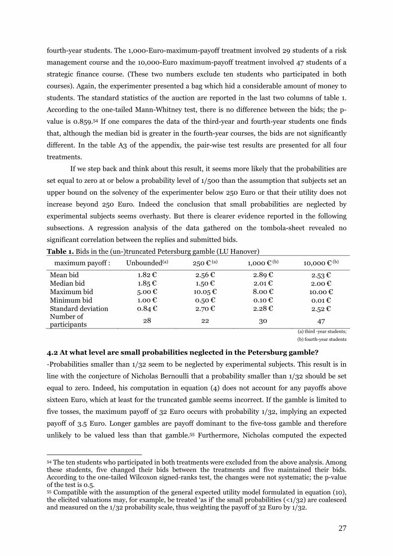
27

fourth-year students. The 1,000-Euro-maximum-payoff treatment involved 29 students of a risk

management course and the 10,000-Euro maximum-payoff treatment involved 47 students of a

strategic finance course. (These two numbers exclude ten students who participated in both

courses). Again, the experimenter presented a bag which hid a considerable amount of money to

students. The standard statistics of the auction are reported in the last two columns of table 1.

According to the one-tailed Mann-Whitney test, there is no difference between the bids; the p-

value is 0.859.54 If one compares the data of the third-year and fourth-year students one finds

that, although the median bid is greater in the fourth-year courses, the bids are not significantly

different. In the table A3 of the appendix, the pair-wise test results are presented for all four

treatments.

If we step back and think about this result, it seems more likely that the probabilities are

set equal to zero at or below a probability level of 1/500 than the assumption that subjects set an

upper bound on the solvency of the experimenter below 250 Euro or that their utility does not

increase beyond 250 Euro. Indeed the conclusion that small probabilities are neglected by

experimental subjects seems overhasty. But there is clearer evidence reported in the following

subsections. A regression analysis of the data gathered on the tombola-sheet revealed no

significant correlation between the replies and submitted bids.

Table 1. Bids in the (un-)truncated Petersburg gamble (LU Hanover)

maximum payoff : Unbounded(a) 250 € (a) 1,000 € (b) 10,000 € (b)

Mean bid 1.82 € 2.56 € 2.89 € 2.53 € Median bid 1.85 € 1.50 € 2.01 € 2.00 € Maximum bid 5.00 € 10.05 € 8.00 € 10.00 € Minimum bid 1.00 € 0.50 € 0.10 € 0.01 € Standard deviation 0.84 € 2.70 € 2.28 € 2.52 € Number of participants

28 22 30 47

(a) third -year students;

(b) fourth-year students

4.2 At what level are small probabilities neglected in the Petersburg gamble?

-Probabilities smaller than 1/32 seem to be neglected by experimental subjects. This result is in

line with the conjecture of Nicholas Bernoulli that a probability smaller than 1/32 should be set

equal to zero. Indeed, his computation in equation (4) does not account for any payoffs above

sixteen Euro, which at least for the truncated gamble seems incorrect. If the gamble is limited to

five tosses, the maximum payoff of 32 Euro occurs with probability 1/32, implying an expected

payoff of 3.5 Euro. Longer gambles are payoff dominant to the five-toss gamble and therefore

unlikely to be valued less than that gamble.55 Furthermore, Nicholas computed the expected

54 The ten students who participated in both treatments were excluded from the above analysis. Among these students, five changed their bids between the treatments and five maintained their bids. According to the one-tailed Wilcoxon signed-ranks test, the changes were not systematic; the p-value of the test is 0.5. 55 Compatible with the assumption of the general expected utility model formulated in equation (10), the elicited valuations may, for example, be treated ‘as if’ the small probabilities (<1/32) are coalesced and measured on the 1/32 probability scale, thus weighting the payoff of 32 Euro by 1/32.

28

value, but admitted that decreasing marginal utility may play a role in the valuation. Therefore

the average valuations should be below the expected value of the five-toss gamble.

To elicit the level at which small probabilities are neglected in the Petersburg gamble, a

field experiment was conducted. The experiment involved 361 participants in six treatments with

the truncated Petersburg gamble. The maximum payoffs in these treatments were 10, 16, 32, 50,

100, and 1,000 Euro, respectively. Participants responded face-to-face to two student researchers

in the students’ restaurant on the campus of the Leibniz University of Hannover. The student

researchers were collecting the data for their graduation in economics between November 2007

and March 2008. The participants were mainly students, i.e. 86.7% were students from all

academic disciplines, 5.3% were employees of the university and 8% were others; 70% of subjects

were male and 30% were female.

The student researchers explained the truncated Petersburg gamble to the participants by

presenting the game tree and a corresponding payoff table in which all possible payoffs and

probabilities were written, not only the first four as in the first classroom study. Participants were

asked for their maximum willingness-to-pay. The student researchers recorded the amount, then

orally repeated the minimum and maximum payoff in the gamble and asked the participant to

confirm the valuation. The participant thus could revise the first answer,56 and the student

researcher offered the gamble for purchase at 5 €. Those participants who agreed to pay this

amount subsequently played the gamble. They repeatedly rolled an ordinary die and bet on the

odd or the even numbers of points before each roll. Table 2 records the descriptive statistics of

this field study. The treatments which involved maximum payoffs of ten Euro or sixteen Euro

elicited a stated median offer of one Euro or two Euro, respectively. The one-tailed Mann-

Whitney test confirms that the difference is significant at the 5% level; the p-value is 0.000. In all

other treatments, the median offer was three Euro. The differences among these other treatments

are not significant at the 5% level, but the offers in those treatments are significantly greater than

in the two aforementioned treatments. Table A4 in the appendix records all pair-wise between-

sample tests. The results thus led to the above observation that smaller probabilities than 1/32 are

neglected in the Petersburg gamble. The observation follows from the fact that the difference

between the 16-Euro-maximum-payoff treatment and the 32-Euro-maximum-payoff treatment is

significant (p-value is 0.018), while the differences between the treatments that involve a

maximum payoff greater than sixteen Euro is not significant. In the 16-Euro-maximum-payoff

treatment, a payoff of sixteen Euro realizes with a probability of 1/16. In the 32-Euro-maximum-

payoff treatment, the payoffs of sixteen Euro and 32 Euro realize each with a probability of 1/32.

Since subjects’ valuations for the two treatments are different, subjects evidently account for the

1/32 probability of winning 32 Euro. On the other hand, as the differences between the 32-Euro-

maximum-payoff treatment and the 50-Euro-maximum-payoff treatment are not significant, one

must conclude that subjects value the chance of winning 32 Euro with a probability of 1/32

equally with the chance of winning 32 Euro or 50 Euro each with a probability of 1/64. This

56 The results reported in this section are based on the revised offers. Nevertheless, the first offers would lead to the same formal observations.

29

probability of winning 50 Euro is apparently judged to be so small that it does not add enough

value to increase subjects’ bids.

In various classroom experiments that I had conducted in different locations, the elicited

willingness-to-pay seemed to exhibit an age effect.57 The more senior students apparently had a

Table 2. Stated willingness-to-pay in the truncated Petersburg gamble (Hannover)

Maximum payoff

10 € a)

16 € a)

32 € a)

50 € a)

100 € a)

1 000 €

a)

Mean offer 1.39 € 2.58 € 3.54 € 3.17 € 4.82 € 5.91 € Median offer 1.00 € 2.00 € 3.00 € 3.00 € 3.00 € 3.00 € Maximum offer 10.00 € 6.00 € 10.00 € 10.00 € 100.00 € 50.00 € Minimum offer 0.00 € 0.00 € 0.00 € 0.00 € 0.00 € 0.00 € Standard deviation 1.55 € 1.61 € 2.34 € 2.00 € 10.98 € 8.86 € Number of participants

50 50 51 50 85 75

higher willingness-to-pay. Therefore, the number of years of studying hereafter referred to as age,

the personal income statistics, gender and other personal details were collected in the field

experiment. The question of monthly income was presented in eight income categories from

which subjects chose one income category rather than stating the exact income. Subjects were

presented with the following income categories in a table; {<300; 300-500; 500-700; 700-1000;

1000-1500; 1500-2000; 2000-2500; >2500}, all amounts in Euro. In total, 352 subjects, or 98.5

percent, replied to the income question. From these data, the following observation can be made;

subject’s offers increase significantly with income (in the treatments that involve a maximum

payoff of at least 32 Euro). For the sample involving the treatments with a maximum payoff of at

least 32 Euro, the pooled regression result of the stated willingness-to-pay on the income

categories is as follows (the asterisk indicates significance at the 5 percent level, the parentheses

quote standard deviations).

stated willingness-to-pay = 2.63* + 0.74* IncCat

(1.013) (0.335)

The regression result is apparently in line with the assumption of Daniel Bernoulli (1954),

according to which the willingness-to-pay for the Petersburg gamble should be an increasing

function of wealth (or income, in line with Marshall 1890). The evidence on the small probability

neglect, however, was not anticipated in Daniel Bernoulli’s theory, as was pointed out by Nicholas

Bernoulli (1732). The other two treatments indicate no significant wage effect, and gender and age

57 A subject-pool effect is very likely. In February and March 2007, I also ran two classroom experiments in Rome at LUISS. The results indicated subject-pool differences; eleven first-year students of a Master of Arts course submitted a median bid of 1.00 Euro for the original (non-truncated) Petersburg gamble, while nine MBA students submitted a median bid of 6.00 Euro for the truncated Petersburg gamble, where the payoff maximum was 100 Euro. The difference is significant; the p-value of the two-tailed Mann-Whitney test is 0.002 (the two-tailed test is used here because of the different subject pools). Actually, the MBA sample elicited significantly higher bids than any other reported classroom experiment.

30

are no significant determinants of the stated willingness-to-pay, either. One should also point out

that the correlation between the stated age and the stated income category is significant in our

sample. The Spearman rank correlation coefficient is 0.260, and the p-value of such an extreme

result is 0.000.

As indicated in the table 3, the stated willingness-to-pay was extraordinarily high in the

field experiment.58 Of the 99 persons who stated an amount at or above five Euro as their

willingness-to-pay, however, only nineteen, or 19 percent, were willing to purchase the gamble at

a price of five Euro. Conversely, four persons, or 1.5 percent, stated an amount below five Euro

and purchased the gamble for five Euro. Eliminating the data points of these subjects does not

lead to different conclusions, but to a lower median willingness-to-pay.

4.3 Is the small probability effect robust to subject-pool changes?

- Yes, it seems to be robust. An additional classroom experiment with an incentive compatible

design was conducted to check the robustness of the results from the field. A total of 232 students

of a third-year economics course59 at the University of Granada, Spain participated in the

experiment. In spring 2008, the course was taught to three different groups by Francis Lagos. At

the end of the final lecture in May 2008, Dr Lagos invited the students to participate in the

experiment and ran on my behalf a second-price auction as described in section 4.1 on the

truncated Petersburg with maximum payoffs 16, 32, and 64 Euro, respectively. In April 2009, the

same course was taught to two different groups by Dr Juan Antonio Lacomba, who invited the

students to participate and conducted two experiments with maximum payoffs of 128 and 1024

Euro. In difference to the German classroom experiment but in line with the field study, all

possible payoffs were presented on the decision sheet and the tombola-sheet was not presented.

The basic statistics of the experiment are reported in the table 3 and the pair-wise test

results are recorded in the table A5 of the appendix. The results replicate the observation of the

field experiment.60 The observed bidding behavior is in line with the hypothesis of Nicholas

Bernoulli (1732), that subjects set small probabilities below 1/32 equal to zero. The between-

country comparison of the bid data for all Petersburg gambles which involve a maximum payoff

above 16 € indicates no differences for the Spanish and German classroom experiments.61

Table 3. Bids in the truncated Petersburg gamble (Granada)

58 The subjects who stated a willingness-to-pay of 50 or 100 Euro as recorded in Table 3 rejected the offer to purchase the gamble at a price of five Euro. 59 Note that third-year economics courses were also implicated in Germany. Thus, cross-country comparison of the bid data may be possible. 60 The one-tailed Mann-Whitney test suggests that the Petersburg gamble truncated at 16 € leads to significantly lower bids than the gamble truncated at 32 €, 64 €, 1024 €; the p-values are 0.041, 0.016, and 0.032, respectively. The sample size of the 128 € cohort is apparently too small to reflect the difference to the 16 € cohort at a 5 percent level; the p-level is 0.095. The pair-wise test results for all the treatments are not significant, they are recorded in Table A5 of the appendix. 61 The two-sample two-tailed Mann-Whitney test does not reject the null hypothesis which assumes no different individual bids in both locations (the p-value is .548), and the eight-sample two-tailed Kruskal-Wallis test does not reject the null of equal bids, either (the p-value is 1.000).

31

maximum payoff : 16 € 32 € 64 € 128 € 1024 €

Mean bid 1.44 € 2.06 € 2.09 € 2.16 € 2.12 € Median bid 1.10 € 1.58 € 1.50 € 1.94 € 2.00 € Maximum bid 5.00 € 8.00 € 10.00 € 7.00 € 6.05 € Minimum bid 0.01 € 0.10 € 0.50 € 0.02 € 0.00 € Standard deviation 1.09 € 1.70 € 1.71 € 1.85 € 1.63 € Number of participants

40 44 59 28 62

5 Concluding remarks

This article reports experimental evidence that people’s elicited willingness-to-pay for the

Petersburg gamble is compatible with the view that subjects neglect small probabilities of

winning. More specifically, the revealed willingness-to-pay for the truncated version of the

Petersburg gamble did not differ from the one for the original version of the gamble. The smallest,

still notable, probability level in the data is 1/32, maybe a surprisingly low level. But this level of

moral impossibility has been proposed by Bernoulli (1732) who, through his continued interest in

the Petersburg gamble, evidenced by persistence in discussing this problem with various

researchers over the years 1713 to 1732, introduced it into the literature. The statistical

equivalence of the willingness-to-pay for the various lengths of the gamble implies that subjects

consider the payoffs up to 32 ducats only. It thus seems reasonable to accept that the neglect of

small probability events is a more relevant decision criterion in the Petersburg gamble than its

best known alternatives, bounded utility (which equalizes the pleasures of gaining 32 ducats with

unlimited wealth) and the limitation of the experimenter’s wealth at 32 ducats. Menger (1934)

pointed out that either an upper bound on utility or a lower bound on probability must be

instigated to resolve the Petersburg paradoxes. Wakker (1993) showed that with denumerable

probability, it is possible to instate a well-defined unbounded utility function. In terms of

probability levels, an equivalent size, namely the 5 percent level, has been proposed by applied

statisticians (following Fisher 1925) as a conservative level of moral impossibility for the social

sciences, since two standard deviations of the distribution are included and only very extreme

outliers are excluded. Indeed, depending on the significance of the subject matter, higher levels of

moral impossibility will be applied. Some consent levels have been established for scientific

research, health care, or forensic proof of evidence. This approach is boundedly rational as the

particular critical probability level seems somewhat arbitrary. Therefore, James Bernoulli (1713)

called for the authorities to fix the levels of moral impossibility, just as rules have been

established for collective or individual safety measures, personal liberty and moral values. As

Nicholas Bernoulli was interested in applying statistics to morals, it is conceivable that the

Petersburg gamble occupied his mind for the exact purpose of fixing the level.

As the discussion on the Petersburg gamble reminds us, it is not prudent to bet large

amounts on extreme outliers in a one-shot game, but in the repeated gamble these extreme

outliers may very well materialize. In this respect the discussion in the paper reiterated that the

one-shot gamble is different from the repeated gamble. Following Laplace (1820), it is perfectly

reasonable for the individual to insure against a personal (unlikely) misfortune, and for the

32

insurance company to insure individuals against such a misfortune. Since the insurance company

frequently takes a gamble on individuals’ misfortunes, the expected value is more relevant to the

insurance company than to the individual who gambles only once. The smaller the probability of

such misfortunes, however, the less frequently do individuals insure against them, as these events

seem too unlikely to occur.62 We have reached the point where we apply both our risk or loss

aversion and the canceling of small probabilities, and eventually we face a trade-off between these

decision rules (Bernoulli 1732; Buffon 1777; Menger 1932; and Kahneman and Tversky 1979).

Coming back to the experimental results, it is observed that most subjects’ elicited willingness-to-

pay falls short of the expected payoff of the gambles.63 This observation is in line with a risk

aversion or a loss aversion argument (Camerer 2007; see also Schmidt and Traub 2002) to which

economists generally would subscribe and has been experimentally supported for the finite

Petersburg gamble by Cox and colleagues (2007, 2008, 2009). Indeed, as Buffon pointed out,

there must be a difference between the pleasure of winning and the pain of losing, so that the

levels of moral impossibility for losses and gains will vary. People weigh small probabilities of

most optimistic outcomes differently from small probabilities of most pessimistic outcomes. As

Samuelson (1977, 42f) puts it: “It is reasonable for me to ignore the small probability that I shall

find a dollar on my way to work.64 But a rational man would not want to ignore the small

probability of a great disaster.” While low probability high impact events have occurred in the

past and are likely to occur in the future, it may be rational to insure against them and prudent to

wager no significant amount on them.

62 The psychological literature has suggested that the perception of small probability events may depend on the experience of their occurrence. Recently experienced events influence decision making, a stylized fact which has been called the recency effect (Robin Hogart and Hillel Einhorn 1992). In recent experimental work it has been shown that the recency effect plays a role in subjects’ decisions to bet on small probability events with repeated gambles (Ralph Hertwig and collaborators 2004). Experimental subjects who do not witness rare events do not bet on them and vice versa. 63 The experimental literature shows that the willingness-to-pay for a lottery is generally smaller than the willingness-to-accept (for a survey see Ulrich Schmidt and Stefan Traub 2009). Given this disparity it is likely that asks are higher under the conditions of a willingness-to-accept procedure. Anticipating that a sale of the Petersburg gamble may lead to considerable losses for the seller, it is also perceivable that the negligence of small probabilities is notable only for much smaller probabilities than 1/32. This issue could be relevant in the explanation of the experimental results by Kroll and Vogt (2009). 64 Presumably, the same story can be told about larger money amounts, too.

33

Appendix

Table A1. Buffon’s results

Number of “tails”

Buffon’s observations

Payoff Buffon’s expectation heuristic a)

0 1061 1 210 = 1024 + 1

1 494 2 29 = 512

2 232 4 28 = 256

3 137 8 27 = 128

4 56 16 26 = 64

5 29 32 25 = 32

6 25 64 24 = 16

7 8 128 23 = 8

8 6 256 22 = 4

9 - 512 21 = 2

10 - 1024 20 = 1

a) Buffon’s expected outcomes match with the geometrical distribution.

34

Table A2. Overview of experimental studies

Session Location Announced

maximum

payoff

Subjects Number of

participants

Median

bid

Session 1 LU. Hannover 10 First year 46 0.10 €

LU. Hannover 100 First year 19 0.99 €

LU. Hannover 1000 First year 22 0.99 €

LU. Hannover ∞ First year 28 0.50 €

Session 2 LU. Hannover 1,000 Fourth year 30 2.01 €

Session 3 LU. Hannover 10,000 Fourth year 47 2.00 €

Session 4 LUISS ∞ First year MA 11 1.00 €

Session 5 LUISS 100 MBA 9 6.00 €

Session 6 LU. Hannover 250 Third year 22 1.85 €

LU. Hannover ∞ Third year 28 1.50 €

Field study LU Hannover 10 50 1.00 €

LU Hannover 16 50 2.00 €

LU Hannover 32 51 3.00 €

LU Hannover 50 50 3.00 €

LU Hannover 100 85 3.00 €

LU Hannover 1000 75 3.00 €

Session 7 U Granada 16 Third year 40 1.10 €

Session 8 U Granada 32 Third year 44 1.58 €

Session 9 U Granada 64 Third year 59 1.50 €

Session 10 U Granada 128 Third year 28 1.94 €

Session 11 U Granada 1024 Third year 62 2.00 €

35

Table A3. Classroom experiment Hannover:

One-tailed Mann-Whitney test results for subjects’ bids

maximum payoff

1,000 € 10,000 € unlimited

250 € .130 .433 .329 1,000 € .859 .904 10,000 € .375

Table A4. Field study:

One-tailed Mann-Whitney test results for subjects’ revised willingness-to-pay

maximum payoff

16 € 32 € 50 € 100 € 1,000 €

10 € .000 .000 .000 .000 .000 16 € .018 .049 .041 .027 32 € .756 .570 .370 50 € .388 .165 100 € .244

Table A5. Classroom experiment Granada:

Mann-Whitney test results for subjects’ bids

maximum payoff

32 € 64 € 128 € 1,024 €

16 € .041 .016 .095 .032 32 € .438 .503 .432 64 € .565 .467 128 € .500

36

References

Aase, Knut. “On the St Petersburg paradox.” Scandinavian Actuarial Journal, pp. 69-78, 2001.

d’Alembert, Jean Le Rond. “Réflexions sur le Calcul des Probabilités.” Opuscules Mathématiques, Tome II, Memoire 10.

Paris 1761-1780, pp. 1-25, 1764.

d’Alembert, Jean Le Rond. “Sur le Calcul des Probabilités.” Opuscules Mathématiques, Tome IV, Paris 1761-1780, 283-310.

1768. Translated by Richard J Pulskamp http://www.cs.xu.edu/math/Sources/Dalembert/memoir27.pdf

d’Alembert, Jean Le Rond. “Sur le Calcul des Probabilités.” Opuscules Mathématiques, Tome VII §2, Paris 1761-1780, 39-

60, 1780.

Allais, Maurice. “The arbitrage between mathematical expectation and the probability of ruin and the St. Petersburg

paradox,” in Maurice Allais and Ole Hagen, eds., Expected Utility and the Allais Paradox. Dodrecht: D. Reidel, pp. 498-

506, 1979.

Arnauld, Antoine and Nicole, Pierre. L’art de penser. (Appeared anonymously.) Paris, 1662.

Arrow, Kenneth J. “Alternative approaches to the theory of choice in risk-taking situations.” Econometrica 19, pp. 404-437,

1951.

Arrow, Kenneth J. Essays in the theory of risk-bearing. Amsterdam and London, pp 44-89, 1971.

Aumann, Robert J. “The St. Petersburg paradox: A discussion of some recent comments.” Journal of Economic Theory 14,

pp. 443-445 , 1977.

Bassett Gilbert W. “The St. Petersburg paradox and bounded utility.” History of Political Economy 19(4), pp. 517-523, 1987.

Bentham, Jeremy. “Rationale of Evidence.” The Works of Jeremy Bentham vol. 6, published under the Superintendence of

his Executor, John Bowring (Edinburgh: William Tait, 1843) 1943.

Berker Istvan ,Csáki Endre and Csörgő Sandor. “Almost sure limit theorems for the St. Petersburg games.” Statistics and

Probabililty Letters. pp. 45, 23-30, 1999.

Bernoulli Daniel. “Specimen theoriae novae de mensura sortis.” Comentarii Academiae Scientarium Imperialis

Petropolitanae V, 175-192, 1738; German translation 1896 by Pringsheim, A, Die Grundlage der modernen Wertlehre.

Versuch einer neuen Theorie der Wertbestimmung von Glücksfällen, Leipzig; English translation 1954 by L. Sommer with

footnotes by Karl Menger, Exposition of a new theory on the measurement of risk, Econometrica 22(1), 23-36; French

translation 1985 Esquisse d'une théorie nouvelle de mesure du sort. Cahiers du séminaire d'histoire des mathématiques, 6,

p. 61-77

Bernoulli, James. The art of conjecturing together with Letter to a friend on sets in court tennis. Translated with an

introduction and notes by Edith Dudley Sylla. The John Hopkins University Press, 2006.

Bernoulli, Nicholas. Letter #18 to Daniel Bernoulli, in B.L. van der Waerden, ed., Die Werke von Jakob Bernoulli 3, K 9.

Basel: Birkhäuser Verlag, pp. 566-568, 1732.

Bernstein, Peter. Against The Gods: the Remarkable Story of Risk, John Wiley & Sons, pp. 106-108, 1996.

Bertrand Joseph. Calcul des probabilities. Paris, pp. 59-64, 1889.

Birnbaum Michael H. “Tests of rank-dependent utility and cumulative prospect theory in gambles represented by natural

frequencies: Effects of format, event framing, and branch splitting.” Organizational Behavior and Human Decision

Processes 95, pp. 40-65, 2004.

Birnbaum, M. H. “Three new tests of independence that differentiate models of risky decision making.” Management Science

51, pp. 1346-1358, 2005 a.

Birnbaum Michael H. “A comparison of five models that predict violations of first-order stochastic dominance in risky

decision making”. Journal of Risk and Uncertainty 31, pp. 263-287, 2005 b.

Brito, D.L. “Becker’s theory of the allocation of time and the St. Peterburg paradox.” Journal of Economic Theory 10(1), pp.

123-26, 1975.

Borel Émile. “Les probabilités dénombrables et leur applications arithmétiques.” Rendiconti del Circolo Matematico di

Palermo 27, pp. 247-271, 1909.

Borel Émile. “Mécanique Statistique et Irréversibilité.” Journal de Physique Théorique et Appliquée 5 (1), pp. 189–196, 1913.

Borel Émile. Le hasard. Paris: Presses Universitaires de France, 1914.

Borel Émile. Valeur pratique et philosophique des probabilités. Paris : Gauthier-Villars, 1939.

Blavatski Pavlo. “Back to the St. Petersburg paradox?.” Management Science 51 (4), pp. 677-678, 2005.

Bottom William P., Bontempo Robert N., Holtgrave and David Robert. Experts, novices, and the St. Petersburg

Paradox: Is one solution enough?.” Journal of Behavioral Decision Making 2, pp. 113-121, 1989.

37

Breiman Leo. “ Optimal gambling systems for favorable games.” Fourth Berkeley Symposium on Mathematical Statistics and

Probability 1, pp. 65-78.

Broome John. "The two-envelope paradox." Analysis 55(1), 6-11.

Bru, B., Bru, M.-F ; and Chung, K.-L. “Borel et la Martingale de Saint-Petersbourg.” Revue d’Histoire des Mathématiques,

5, pp. 181–247, 1999.

Budescu David V. and Amnon Rapoport. “Generation of random series in two-person strictly competitive games.” Journal

of Experimental Psychology 121(3), pp. 352-363, 1992.

Buffon Georges-Louis Leclerc. “Essai d’arithmétique morale.” in Supplément à l’historie naturelle IV, reproduced in Un

autre Buffon, Hermann, 1977, pp. 47-59, 1777.

Camerer Colin. “Three Cheers—Psychological. Theoretical, Empirical—for Loss Aversion.” Journal of Marketing Research

42(2), pp. 129-134, 2005.

Ceasar Allan J. “A Monte Carlo Simulation Related to the St. Petersburg Paradox.” College Mathematical Journal, 15 (4) pp.

399-342, 1984.

Cardano Girolamo. Practica arithmeticae. Milano: 1539.

Chipman J.S. Foundations of utility.” Econometrica 28, pp. 193-224, 1960.

Condorcet M. Essai sur l’application de l’analyse á la probabilité des decisions rendues à la pluralité des voix. Paris: De

l’imprimerie royale, 1785.

Coolidge J.W. The mathematics of great amateurs. New York: Dover Publications [1949], 1963.

Cournot Antoine Augustin. Exposition de la théorie des chances et des probabilities. Paris, L. Hachette, 1843.

Cox, James C.; Sadiraj, Vjollca; Vogt, Bodo, and Dasgupta, Utteeyo. “Is there a plausible theory for risky decisions?.”

Georgia State University, Experimental Economics Center Working Paper 2007 – 05, 2007.

Cox, James C., and Sadiraj, Vjollca. “Risky decisions in the large and in the small: theory and experiment,” in: Cox, James

C. and Harrison, Glenn W. (eds.) Risk Aversion in Experiments, Research in Expermental Economics 12, pp. 9-40, 2008.

Cox, James C., Sadiraj, Vjollca, and Vogt, Bodo. “On the Empirical Relevance of St. Petersburg Lotteries,” Economics

Bulletin, Vol. 29(1), pp. 221-227, 2009.

Cramer Gabriel. “Letter to N. Bernoulli.” 1928. Published fully in Daniel Bernoulli, 1954, pp. 33-35.

Csörgő Sándor. Nicholas Bernoulli, in: Heyde, C.C., Seneta, Eugene (eds.) Statisticians of the Centuries, Springer, pp. 55-63,

2001.

Csörgő Sándor. 2003 “Merge Rates for Sums of Large Winnings in Generalized St. Petersburg Games,” Acta Scientiarum

Mathematicarum (Szeged), 69, pp. 441–454, 2003.

Csörgő Sándor and Simons Gordon. “On Steinhaus’ Resolution of the St. Petersburg Paradox,” Probability and

Mathematical Statistics. 14, pp. 157–172, 1993–1994.

Csörgő Sándor and Simons Gordon. “A Strong Law of Large Numbers for Trimmed Sums, with Applications to

Generalized St. Petersburg Games,” Statistics & Probability Letters. 26, pp. 65–73, 1996.

Csörgő Sándor and Simons Gordon. “The Two-Paul Paradox and the Comparison of Infinite Expectations,” in Limit

Theorems in Probability and Statistics, eds. I. Berkes et al., Budapest: János Bolyai Mathematical Society, pp. 427–455,

2002.

Csörgő Sándor and Simons Gordon. Laws of large numbers for cooperative St. Petersburg gamblers, Volume 50,

Numbers 1-2 / August 2005.

Czuber Emanuel. “Das Petersburger Problem. ”Archiv der Mathematik und Physik 67, pp. 1-28, 1882.

Daston L. “Probabilistic Expectation and Rationality in Classical Probability Theory.” Historia Mathematica, 7, pp. 234-60,

1980.

Descartes, René; Cottingham, John; Stoothoff, Robert; Murdoch, Dugald Kenny and Anthony John Patrick.

“The Philosophical Writings of Descartes.” Cambridge University Press, 1985.

Devlin Keith. The unfinished game. NY: Basic Books, 2008.

Ducel Yves and Martin Thierry. “Georges-Louis Leclerc.” Comte de Buffon, in: Heyde, C.C., Seneta, Eugene (eds.)

Statisticians of the Centuries, Springer, pp. 77-81, 2001.

Dudley-Silla David. “Growth Stocks and the Petersburg Paradox.” Journal of Finance 12: pp. 348-63, 1957.

Durand David. “Growth Stocks and the Petersburg Paradox.” Journal of Finance 12: pp. 348-63, 1957.

Dutka Jacques. “On the St. Petersburg paradox.” Archive History of Exact Sciences 39, pp. 13-39, 1988.

Edgeworth, Francis Y. Mathematical Psychics: An Essay on the Application of Mathematics to the Moral Sciences. London

1881.

38

Edwards Ward. “The theory of decision making.” Psychological Bulletin. 51, 380–417, 1954.

Euler Leonhard. “Vera aestimatio sortis in ludis.” Opera posthuma 1, pp. 315-318, 1862. Translation by Richard Pulskamp

titled “The true valuation of the risk in games” available at http://www.cs.xu .edu/math/Sources/Euler/E811.pdf

Feller William. “Note on the Law of Large Numbers and ‘Fair’ Games.” Annals of Mathematical Statistics. 16, 301–304, 1945.

Fontaine Alexis. “Solution d’un probleme sur les jeux de hazard.” Mémoires donnés à l’Acad. Roy. Des Sciences, 429-431,

1764.

Fréchet Maurice. “L’estimation statistique des paramètres abstract.” Econometrica 16, 60-62, 1948.

Fries Jakob Friedrich. “Versuch einer Kritik der Principien der Wahrscheinlichkeitsrechnung.” Braunschweig, pp. 114-120,

1842.

Fry Thornton C. Probability and its Engineering uses. New York: Van Nostrand, 194-199, 1928.

Fishburn Peter C. “Expected utility: An anniversary and a new era.” Journal of Risk and Uncertainty 1(3) 1988.

Furlan L.V. “Bemerkungen zum Petersburger Problem.” Schweizerische Zeitschrift für Volkswirtschaft und Statistik 82, pp.

444-448, 1946.

Gorovitz Samuel. “The St. Petersburg paradox,” in Maurice Allais, Ole Hagen (eds.) Expected Utility and the Allais Paradox,

pp. 259-270, 1979.

Gordon M.J. “The Investment.” Financing and Valuation of the Corporation, Homewood. Illinois: Richard D. Irwin, Inc.

1962.

Gottinger H.W. “Bernoulli’s utility theory and historical ramifications.” Jahrbücher für Nationalökonomie und Statistik 186,

481-497, 1971/72.

Hacking Ian. “The emergence of probability and inductive logic.” Cambridge University Press, pp. 91-100, 2001.

Haller Helmut H. “Mixed extension of games and the Saint Petersburg paradox.” In R. Nau et al. (ed.) Economic and

Environmental Risk and Uncertainty. PP. 163-171.

Hardin Russell. “Collective Action.” The Johns Hopkins University Press. 1982.

Hastie Reid. “Algebraic models of juror decision processes,” in Reid Hastie, Lola L. Lopes, Hal R. Arkes (eds.) Inside the

Juror, NY: Cambridge University Press. pp. 84-115, 1993.

Hayden, B.Y. and Platt, M.L. “The Mean, the Median, and the St. Petersburg Paradox,” Judgment and Decision Making, Vol.

4 (4), 256-272, 2009.

Hertwig, Ralph; Barron, Greg; Weber, Elke U., and Erev, Ido. “Decisions From Experience and the Effect of Rare

Events in Risky Choice.” Psychological Science 15(8), pp. 534-39, 2004.

Hinners-Tobrägel Ludger. “The St. Petersburg paradox.” Paper presented at the EFITA 2003 Conference.

Hogarth Robin and Einhorn Hillel. “Order effects in belief updating: The belief-adjustment model.” Cognitive Psychology,

24, pp. 1-55, 1992.

Jallais S. and Pradier P.-C. “L'erreur de Daniel Bernoulli ou Pascal incompris.” Economies et Sociétés, OEconomia. 25, pp.

17-48, 1997.

Jeffrey Richard C. “The logic of decision.” McGraw Hill, New York, 1965.

Jerger Jürgen. “Das St. Petersburger Paradoxon.” - WiSt 21, number 8, pp. 407-410, 1992.

Joyce J. Foundations of Causal Decision Theory. Cambridge: Cambridge University Press. 1999.

Jorland Gerard. “The Saint Petersburg Paradox, 1713-1937.” In Michael Heidelberger, Lorenz Krüger, and Rosemarie

Rheinwald (Eds.), Probability since 1800. Bielefeld: Wissenschaftsforschung B.K. Verlag GmbH. 1983.

Jorland Gerard. “Probability, the theory of games and economics.” The Saint Petersburg Paradox. In L. Krüger, L. Daston &

L. Heidelberger (Eds.), The Probabilistic Revolution. Vol.1, pp. 157-90, 1987. Cambridge (Mass.): The MIT Press.

Keynes John M. A treatise on probability. London: MacMillan and Co. 1921.

Kinsch Patrick. “Probabilité et certitude dans la preuve en justice.” Institut Grand-Ducal Actes de la Section des Sciences

Morales et Politiques, pp. 65-103, 2008.

Kohli Karl. “Spieldauer,” in B.L. van der Waerden (ed.): Die Werke von Jakob Bernoulli 3, K 4. Basel: Birkhäuser Verlag. Pp.

403-456, 1975.

Knobloch Eberhard “Emile Borel as a Probabilist,” In L. Krüger, L. Daston & L. Heidelberger (Eds.), The Probabilistic

Revolution. Vol.1, pp. 215-33. Cambridge (Mass.): The MIT Press, 1987.

Kraitchik M. "The Saint Petersburg Paradox", §6.18 in Mathematical Recreations. W. W. Norton. 1942.

Kroll, Eike Benjamin and Vogt, Bodo. “The Petersburg Paradox Despite Risk-Seeking Preferences: An Experimental

Study” FEMM working paper No. 4, January 2009.

Lacroix Sylvestre François. Traité du calcul différentiel et du calcul intégral. Paris : Chez Courcier. 1802.

39

Laplace Pierre-Simon. “Théorie analtytique des probabilités.” Livre II, Chapitre X. De l’espérance morale, Oeuvres de

Laplace, ome VII, Imprimerie Royale, 1847, pp. 474-488, 1812.

Laplace Pierre-Simon. “Essai philiosophique sur les probabilités.” 2 Vols., Paris, Gauthier-Villars, Vol 1, pp. 22-23, 1921.

Levy Paul. “Calcul des probabilities.” Chapitre VI, Critique de la théorie du gain probable, Gauthier-Villars, Paris, 1925, 113-

133.

Lopes Lola L. “Decision making in the short run.” Journal of Experimental Psychology: Human Learning and Memory, 7,

pp. 377-385, 1981 .

Luce R. Duncan and Suppes Patrick. “Representational measurement theory,” in Stevens’ Handbook of Experimental

Psychology, Vol. 4, 3rd Edition, H. Pashler, ed., Wiley, New York, pp. 1–41, 2002.

Lupton Sydney. “The St. Petersburg Problem.” Nature Vol. 41, pp. 168-169, 1890.

Markowitz Harry M. “Portfolio selection.” Journal of Finance 7(1), 77-91, 1952.

Martin Thierry. “La logique probabiliste de Gabriel Cramer.” Mathématiques et sciences humaines ~ Mathematics and Social

Sciences 176(4), pp. 43-60, 2006.

Martin-Löf Anders. “A Limit Theorem Which Clarifies the ‘Petersburg Paradox.” Journal of Applied Probability, 22, pp.

634–643, 1985.

Martin-Löf Anders. “An analysis of two modifications of the Petersburg game and of another game allowing arbitrage.”

Mathematical Statistics Stockholm University Research Report 2001:11, November 2001.

Marshall, Alfred. Principles of Economics London: Macmillan and Co., Ltd., 1890.

Menger Karl. “Das Unsicherheitsmoment in der Wertlehre.“ Zeitschrift der Nationalökonomie 51, pp. 459-485, 1934. English

translation by Wolfgang Schoellkopf with assistance of W. Giles Mellon. The role of uncertainty in economics, Chapter 16

in Essays in mathematical economics in honor of Oskar Morgenstern, Princeton: Princeton University Press, pp. 211-232,

1967.

Montmort Raimond. 1713, (anonymously published): Essay d’Analyse sur les Jeux de Hazard, Quillaud, Paris, first edition

appeared in 1708 ; second edition includes important letters by John and Nicholas Bernoulli. Reprinted by the American

Mathematical Society Chelsea Publishing, Rhode Island, 2006.

Pareto, Vilfredo F. “Considerazioni sui principii fondamentali dell'economia politicapura V.” Giornale degli Economisti 2(7),

279-321, October 1893.

Plous, Scott. The psychology of judgment and decision making, McGraw-Hill, pp. 79ff, 1993.

Poisson Simeon-Denis. “Recherches sur la probabilité des jugements en matières criminelles et matière civile (4to, 1837).”

All published at Paris. A translation of Poisson's Treatise on Mechanics was published in London in 1842.

Quiggin John. “A theory of anticipated utility.” Journal of Economic Behavior and Organization. 3, pp. 324–345.

Ramsey, Frank P. “Truth and Probability,” in Frank Ramsey and Richard Bevan, eds., The Foundations of. Mathematics and

other Logical Essays Ch. VII, pp. 156-198, 1931.

Restle Frank. Psychology and judgment of choice. New York: John Wiley & Sons, pp.107-135, 1961.

Rieger Marc Oliver and Wang Mei. “Cumulative prospect theory and the St. Petersburg paradox.” Economic Theory. 28(3),

pp. 665-679, 2006.

Rivero J.C., Holtgrave David R., Bontempo Robert N. and Bottom William P. “The St. Petersburg Paradox: Data, at

last.” Commentary, 8: pp. 46-51, 1990. Reprinted in W. H. Loke (ed.) Perspectives on Judgment and Decision Making,

Lanham Press: Kent, England.

Rump Christopher M. “Capital Growth and the St. Petersburg Game.” The American Statistician. 61(3), pp. 213-217, 2007.

Russon Manuel G. and Chang SJ. "Risk aversion and practical expected value: A simulation of the St Petersburg Game."

Simulation & Gaming, 23, pp. 6-19, 1992.

Samuelson Paul A. “The St. Petersburg Paradox as a Divergent Double Limit.” International Economic Review. 1, pp. 30-37,

1960.

Samuelson Paul A. “A Fallacy of Large Numbers.” Scientia 98, pp. 108-113, 1963.

Samuelson Paul A. “St. Petersburg Paradoxes: Defanged, Dissected and Historically Described.” Journal of Economic

Literature. 15(1), pp. 24-55, 1977.

Sandifer Ed. “How Euler did it – St. Petersburg Paradox.” Internet resource,

http://www.maa.org/editorial/euler/how%20euler%20did%20it%2045%20st%20petersburg%20paradox.pdf, 2004.

Schmidt, Ulrich and Traub, Stefan. “An Experimental Investigation of the Disparity Between WTA and WTP for

Lotteries,“ Theory and Decision 66(3), pp. 229-262, March 2009.

40

Schmidt, Ulrich and Traub, Stefan. “An Experimental Test of Loss Aversion,“ Journal of Risk and Uncertainty 25, pp.

233-249, 2002.

Schredelseker, Klaus. Grundlagen der Finanzwirtschaft Ein informationsöko-nomischer Zugang. Oldenbourg:

Wissenschaftsverlag, pp. 220-21, 2002.

Selten, Reinhard. “What is bounded rationality? In Gigerenzer, Gerd and Selten, Reinhard, eds., Bounded rationality: the

adaptive tool box. The MIT Press, pp. 13-36, 2001.

Senetti J.T. “On Bernoulli, Sharpe, financial risk, and the St. Petersburg paradox.” Journal of Finance 31, pp. 960-962, 1976.

Shafer, Glenn. The St. Petersburg paradox. In Samuel Kotz and Norman L. Johnson, eds., Encyclopedia of statistical sciences

8, pp. 865-870, 1988.

Shapiro, Barbara J. Beyond reasonable doubt and probable cause – historical perspectives on the Anglo-American law of

evidence. Berkeley: University of California Press, 1991.

Shapley, Lloyd. S. “The Petersburg Paradox – A con game ?” Journal of Economic Theory 14, pp. 439-442, 1977.

Shefrin, Hersh. Bey0nd Greed and Fear, Oxford University Press, 2002.

Sheynin, Oscar. “On the early history of the law of large numbers.” In Editors, Egon S. Pearson and Maurice G. Kendall, eds.,

Studies in the History of Statistics and Probability [vol. 1]. London, pp. 231–239, 1970.

Sinn, Hans-Werner. Ökonomische Entscheidungen bei Ungewissheit, Tübingen: Mohr, pp. 194-197, 1980.

Spiess, Otto. „Zur Vorgeschichte des Petersburger Problems,“ in B.L. van der Waerden (ed.): Die Werke von Jakob Bernoulli

3, K 9. Basel: Birkhäuser Verlag, 557-568. (translated to English in Pulskamp Richard J. “Correspondence of Nicolas

Bernoulli concerning the St. Petersburg Game,” Internet resource,

http://cerebro.xu.edu/math/Sources/Montmort/stpetersburg.pdf, 1999.), 1975.

Spremann, Klaus. “Why black swans exist,” in Michael Hanke and Jürgen Huber, eds., Information, Interaction and

(In)Efficiency in Financial Markets, Vienna: Linde, pp. 170-181, 2008.

Starmer, Chris. “Developments in Non-Expected Utility Theory: The Hunt for a Descriptive Theory of Choice under Risk.”

Journal of Economic Literature 38, pp. 332–382, 2000.

Stigler, George J. “The development of utility theory II.” Journal of Political Economy 58(4), pp. 373-396, 1950.

Stigler, Stephen M. The History of Statistics : the measurement of uncertainty before 1900, Cambridge MA, 1986.

Sundali, James and Croson, Rachel. “Biases in casino betting: The hot hand and the gambler's fallacy.” Judgment and

Decision Making 1(1), pp. 1-12, July 2006.

Székely, Gabor and Richards, Donald St. P. “The St. Petersburg paradox and the crash of high-tech stocks in 2000", The

American Statistician 58, pp. 225-31, 2004.

Székely, Gabor and Richards, Donald St. P. “Remain Steadfast with the St. Petersburg Paradox to Quantify Irrational

Exuberance”, mimeo, Penn. State University, Dept. of Statistics, June 27, 2005.

Taleb, Nassim Nicholas. The Black Swan: The Impact of the Highly Improbable. New York: Random House, 2007.

Todhunter, Isaac. Mathematical theory of probability – From the time of Pascal to that of Laplace. Cambridge and London:

MacMillan and Co, 1865.

Treisman, Michel. “A solution to the Petersburg paradox.” British Journal of Mathematical and Statistical Psychology 9, pp.

224-227, 1983.

Tyler Cowen and Jack High. “Time, bounded utility, and the St. Petersburg paradox.” Theory and Decision 25, Number 3 ,

pp. 219-223, November 1988.

Vickrey William Spencer. “Counterspeculation, auctions, and competitive sealed tenders.” Journal of Finance. 16, pp. 8-37,

1961.

Vivian Robert William. “Simulating Daniel Bernoulli’s St. Petersburg game: Theoretical and empirical consistency.”

Simulation & Gaming. Vol. 35(4), pp. 499-504, 2004.

Wakker P. “Unbounded Utility for Savage’s ‘Foundations of Statistics,’ and Other Models.” Mathematics of Operations

Research. 18, pp. 446-485, 1993.

Weaver Warren. Lady Luck. New York: Anchor Books. 1963.

Weber, Max. “Die Grenznutzlehre und das "psychophysische Grundgesetz.” Archiv für Sozialwissenschaft und Sozialpolitik

27, 546-58, 1908.

Weirich Paul. “The St. Petersburg Gamble and Risk’.” Theory and Decision. 17, pp. 193-202, 1984.

Whitworth William Allan. Choice and Chance. Second edition, Cambridge: Deighton. Bell and Co., pp. 222-230, 1870.

Wicksell, Knut. “Zur Verteidigung der Grenznutzenlehre.” Zeitschrift für die gesamte Staatswissenschaft 56(4), pp. 577-91,

1900.

41

Yaari Menahem E. “The Dual Theory of Choice Under Risk,” Econometrica. 55, pp. 95–115, 1987.

42

INSTRUCTIONS You are about to participate in an economic experiment. During the experiment, please do not talk to anyone. Please make your decision on your own and follow the instructions carefully. It is in your own interests that you understand the instructions. GENERAL INFORMATION In the experiment, you are asked to submit a bid for a gamble that has a monetary payoff. You write your bid and your name on your sheet of paper which will be collected later. The participant who submits the highest bid wins the gamble, and will pay to us the second highest bid; the other participants will not win anything and will not pay anything. The winner plays the gamble and earns the monetary payoff of the gamble. The money amount will be paid out immediately. Please note that the winner of the gamble pays a price for the gamble which may be higher than the money that he or she wins in the gamble. Therefore we advise you to choose your bid carefully. There will be no refund, if you make a loss! You bid on the following gamble. THE GAMBLE There are two balls in a bag. The balls are identical except for the label. One ball is labelled with ‘+’, the other is unlabelled. You draw one ball from the bag. If you draw the ball labelled ‘+’ it is returned into the bag and you draw again. Each time you draw the ‘+’ labelled ball it will be recorded. The game continues until you draw the unlabelled ball for the first time. Then the gamble stops and you receive your payoff according to the recorded number of ‘+’ draws that you have made. Let this number be denoted by k. Then your payoff from the gamble is 2k Euro. In words: Your payoff is two Euro to the power of the number of times you draw the ‘+’ labelled ball. For k ≤ 5, the resulting payoffs are presented in the following table.

Your sequence of draws Your payoff in € 20 = 1 + 21 = 2 ++ 22 = 4 +++ 23 = 8 ++++ 24 = 16 +++++ 25 = 32 ….

Notice, of course, that k may be more or less than 5. Indeed, k could be very large. Your minimum payoff in the gamble is 1 Euro. There is no maximum payoff in the gamble. Only one participant wins the gamble and plays it out. The price this participant has to pay for the participation in the gamble is determined by the second highest bid submitted in the auction. Please write your bid in the space at the end of this sheet of paper. You will privately submit your bid without knowing the bids of the other participants. Your bid should be your maximum willingness-to-pay (in Euro) for participation in the gamble; if your bid is the highest bid, the price you pay will not exceed your bid but it might equal your bid. All bids shall be in Euro, decimals after the comma indicate Eurocents. The smallest unit one can bid is 0,01 Euro and 0,01 Euro is also the minimum bid for the gamble. After all bids have been collected, the winner in the auction will be determined. The gamble will be assigned to the participant who submitted the highest bid. In case of a draw, that is, if several participants submit the highest bid, the winner will be determined by randomly selecting one of the highest bidders. As we have already said, the price the winner pays for the gamble equals the second highest bid. Unless there is more than one high bidder, the price will be smaller than the highest bid. Example: Assume one participant submits a bid of 0,02 Euro and the second participant bids 0,03 Euro while all other participants submit a bid equal to 0,01 Euro. The second bidder wins the gamble and pays the second highest price of 0,02 Euro. If the second participant submits a bid of 0,02 Euro instead, her/his bid is equal to the bid of the first participant. The winner, either participant 1 or 2, must be determined through a random draw. The price the winner pays, i.e., the second highest bid, is then equal to her/his own bid of 0,02 Euro. Write your name here: Write your bid here: , Euro Comment: FURTHER INSTRUCTIONS The winner of the gamble will be determined, and the gamble will be played out. The winner will draw balls from the bag (with replacement) until the unlabeled ball shows up. GENERAL INFORMATION On this sheet you are asked to reply to three further questions regarding the outcomes of the gamble. The first question will ask you to state three outcomes. The second and the third are quiz questions. This sheet of paper represents your lot for a tombola. If your lot (i.e., this sheet) is drawn in the tombola and your answer is correct you win 10 Euro, otherwise you win nothing. In total, the tombola involves 3 draws (with replacement) from the lots (i.e., sheets) of all participants. In other words, after each draw the drawn lot is returned to the other lots to participate in the next tombola. QUESTIONS

43

1) One lot will be drawn (with replacement) after the gamble has been played out. The number of times the ‘+’ labelled ball has been drawn in the gamble will be compared with the three outcomes you state on this sheet (if your sheet is drawn). If the sequence length that has realized in the gamble coincides with one of the three numbers you state below and your lot is drawn in the tombola, you win 10 Euro. Please write down here the three non-negative numbers: k1 = k2 = k3 = 2) The second lot will be drawn next. The number of draws of the ‘+’ labelled ball that has a (mathematical) probability of 1/128 will be compared to the number you state below. You win 10 Euro on this question, if your lot is drawn and your reply is correct. k = 3) Finally, the third lot will be drawn. The number you state hereafter will be compared to the expected payoff of the gamble. If your answer is correct and your lot is drawn, you win 10 Euro on this question. Expected payoff in the gamble = Write your name here: