DIGITAL-MODEL SIMULATION OF THE TOPPENISH ALLUVIAL AQUIFER, YAKIMA INDIAN RESERVATION,

WASHINGTON U.S. GEOLOGICAL SURVEY Water-Resources Investigations Open-File Report 81-425

1111 111 811111111:1[IIR0018911 81

UNITED STATES DEPARTMENT OF THE INTERIOR

GEOLOGICAL SURVEY

DIGITAL-MODEL SIMULATION OF THE

TOPPENISH ALLUVIAL AQUIFER,

YAKIMA INDIAN RESERVATION,

WASHINGTON

By E. L. Bolke and J. A. Skrivan

U. S. GEOLOGICAL SURVEY

WATER-RESOURCES INVESTIGATIONS

OPEN-FILE REPORT 81-425

Prepared in cooperation with the Yakima Tribal Council

(‘• OT191RvEi• it OCT 151981

13R KO-4/

'tat Tr Olerc:‘

Tacoma, Washington Ck.Vii;ed S 1981 Ger)109,\C&

UNITED STATES DEPARTMENT OF THE INTERIOR

JAMES G. WATT, Secretary

GEOLOGICAL SURVEY

Doyle G. Frederick, Acting Director

Cover painting by Fred Oldfield. Mr. Oldfield was born and raised on the Yakima Indian Reservation. Covers furnished by Yakima Tribal Council.

For additional information write to:

U.S. Geological Survey 1201 Pacific Avenue - Suite 600 Tacoma, Washington 98402

CONTENTS

Page

Abstract--- 1 Introduction 2

Purpose and scope 2 Description of the study area 4 Previous investigations 6 Acknowledgments 6 Numbering system for wells and streamflow-data sites 7

Hydrogeology 8 Setting 8 Extent and thickness of the aquifer 8 Precipitation 11 Evapotranspiration 11 Ground-water pumpage 11 Ground-water movement 13 Water-level fluctuations in the aquifer 13

Hydraulic characteristics of the aquifer 16 Lateral hydraulic conductivity 16 Vertical hydraulic conductivity of confining beds 16 Transmissivity and specific yield 18 Aquifer-stream connection 18

Model construction and calibration 20 Model boundaries 20 Model input 22 Time-averaged simulation 23 Transient simulation 26 Sensitivity 30

Model utilization 31 Summary and conclusions 33 Recommendations for future studies 33 References 34

ILLUSTRATIONS

Page

FIGURES 1-14. Maps showing: 1. Location of the study area 3 2. Location of streams, canals, drains, and

associated data sites 5 3. Generalized geology of the study area 9 4. Saturated thickness used in the model

of the Toppenish alluvial aquifer 10 5. Location of selected wells and rates

of major ground-water pumpage 12 6. Water-table configuration of the Toppenish

alluvial aquifer, March 1972 14 7. Seasonal water-level changes in the

Toppenish alluvial aquifer and monthly diversions to the Main Canal from the Yakima River 15

8. Lateral hydraulic conductivity used in the model 17

9. Transmissivity used in the model 19 10. Model grid network and boundary conditions

used in the model 21 11. Average observed and model-calculated

water-table configuration during 1971-72 24

12. Observed and calculated water-table configuration as determined from transient simulation for September 1971- 27

13. Observed and calculated water-table con- figuration as determined from transient simulation for March 1972 28

14. Distribution of water-level decline due to hypothetical pumping stress 32

TABLES

TABLE 1. Water budget for' the time-averaged simulation 25 2. Water budget for the transient simulation 29

iv

METRIC (SI) CONVERSION FACTORS

Multiply To obtain

foot (ft) inch (in.) acre-foot (acre-ft) mile (mi) square mile (mi2) cubic foot pr second (ft /s)

square foot per second (ft/s)

0.3048 25.4 0.001233 1.609 2.590 0.02832

0.0929

meter (m) millimeter (mm) cubic hectometer (hm3) kilometer (km) square kilometer (km2) cubic meter per second (m3/s)

square meter per second (m2/s)

National Geodetic Vertical Datum of 1929 (NGVD of 1929): A geodetic datum derived from a general adjustment of the first-order level nets of both the United States and Canada, formerly called "Mean Sea Level."

NGVD of 1929 is referred to as sea level in this report.

DIGITAL-MODEL SIMULATION OF THE TOPPENISH ALLUVIAL AQUIFER,

YAKIMA INDIAN RESERVATION, WASHINGTON

By E. L. Bolke and 3. A. Skrivan

ABSTRACT

Increasing demands for irrigating additional lands and proposals to divert water from the Yakima River by water users downstream from the Yakima Indian Reservation have made an accounting of water availability important for present-day water management in the Toppenish Creek basin. A digital model was constructed and calibrated for the Toppenish alluvial aquifer to help fulfill this need. The average difference between observed and model-calculated aquifer heads was about 4 feet. Results of model analysis show that the net gain to the aquifer from the Yakima River is 90 cubic feet per second, and the net loss from the aquifer to Toppenish Creek is 137 cubic feet per second. Water-level declines of about 5 feet were calculated for an area near Toppenish in reponse to a hypothetical tenfold increase in 1974 pumping rates.

1

INTRODUCTION

The Toppenish Creek basin in the Yakima Indian Reservation in south-central Washington (fig. 1) contains abundant arable soils and, due to its dry climate, relies heavily on irrigation for crop production. Currently, sufficient water for irrigation is available from diversions of the Yakima River, Toppenish Creek, and from ground-water supplies. Increasing demands for irrigating additional lands and proposals to divert water from the Yakima River by water users downstream from the reservation have made an accounting of water availability important for present-day water management in the basin. Recognizing the need to evaluate various ground-water-management alternatives, the Yakima Tribal Council entered into a cooperative agreement with the U.S. Geological Survey to construct digital-computer models to test the effects of stresses on the ground-water system in the Toppenish Creek basin. A previous Geological Survey study (Skrivan, written commun., 1980) documents the first such model, which was designed primarily to be used in management of basalt aquifers in the basin. This report describes the development of the model for the alluvial aquifer.

Purpose and Scope

The purpose of this study was to: (1) describe the hydrologic setting and hydraulic characteristics of the Toppenish Creek alluvial aquifer; and (2) construct and cali5rate a digital model to simulate movement of water in the aquifer and between the aquifer and the Yakima River and Toppenish Creek. The study was made by the U.S. Geological Survey in cooperation with the Yakima Tribal Council.

The study is based in part on data collected in the field, and on data and results from a water-resources appraisal of the Toppenish Creek basin (U.S. Geological Survey, 1975) and historical data available in the files of the U.S. Geological Survey, Tacoma, Wash. The study period was from March 1971 to March 1973.

2

Cascade Range

WASHINGTON

Union Gap

120°35 ► 22 30

46°30 4-

Boundary of study area

tO

Wapato

Harrah

Toppenish

46°20' -4- eek

Toppenish Ridge 0 1 2 3 MILES

I III 1' 0 1 2 3 4 KILOMETERS

FIGURE 1.--Location of the study area.

3

Description of the Study Area

The study area is located in the Toppenish Creek drainage basin in the Yakima Indian Reservation, Yakima County, on the eastern slope of the Cascade Range (fig. 1). Geologically, the study area comprises an alluvial fan with its apex near Union Gap, extending south to the base of Toppenish Ridge. The eastern boundary extends along the Yakima River from Union Gap to its confluence with Toppenish Creek, and the western boundary extends southwest from Union Gap to near Harrah and then south to Toppenish Ridge. The study area ranges in width from 1 to 20 mi and covers about 175 mi2. The area covered by the digital model is about 166 mi2.

Toppenish Creek, the major tributary to the Yakima River in the study area, enters the area near the southwest corner and flows eastward along the southern boundary until it discharges into the Yakima River near the southeast corner. Both Toppenish Creek and the Yakima River are perennial streams. Their st-earnflow characteristics are detailed in U.S. Geological Survey (1975).

Diversions from the Yakima River near Union Gap supply a canal system that provides irrigation water for about 78,000 acres over the alluvial aquifer, and makes agriculture the principal industry in the area. Annual diversions from Main Canal and \Vanity Slough provide about 475,000 acre-ft of irrigation water to the area. An additional 6,000 acre-ft per year is pumped from the alluvial aquifer. The canal system covers virtually the entire study area (fig. 2). Near-surface soils are drained by an extensive system of ditches (drains) that route the excess irrigation water to either Toppenish Creek or the Yakima River. Some of the water from Toppenish Creek is diverted from near its mouth to the Satus Creek drainage basin south of the study area.

The climate in the study area is semiarid, with an annual average precipitation of 7 in. About 10,000 people live in the area, primarily in Toppenish, Wapato, and Harrah (fig. 1).

4

EXPLANATION 0 120°35' 22'30"

46 30' Miscellaneous streamflow site

• Continuous flow record site

(canals and drains)

4 Main Canal Diversion

-- Canal

--- Drain

Main canal

p 1 2 3 MILES

I 1 1

I 0 1 2 3 4 KILOMTERS

12507040

120°10'

12507500

FIGURE 2.--Location of streams, canals, drains, and associated data sites.

Previous Investigations

Early reports by Russell (1893), Smith (1901, 1903), and Waring (1913) discussed the geology and general distribution of ground water in the area. Kinnison and Sceva (1963) studied the effect of geology on streamflow in the Yakima River. A water budget for Toppenish Creek basin, which included both surface- and ground-water hydrology in the area, was determined by the U.S. Geological Survey (1975). Skrivan (U.S. Geological Survey, written commun., 1980) constructed a digital model of the lower confined aquifers of the Toppenish Creek basin.

Acknowledgments

We thank personnel of the U.S. Bureau of Indian Affairs (BIA), the Yakima Agency Staff of BIA, and the Wapato Irrigation Project Office of BIA for providing data on ground-water levels and surface-water diversions within the project area. Funding for the study was provided by the Yakima Tribal Council and the U.S. Geolgocial Survey.

6

Numbering System for Wells and Streamflow Data Sites

Wells in Washington are assigned numbers identifying their location within a township, range, and section. Well number 11/19-17R1 indicates, successively, the township (T.11 N.), and range (R.19 E.), north and east of the Willamette base line and meridian; because of all wells in this report are north and east of the Willamette base line and meridian, the letters indicating north and east are omitted. The first number following the hyphen indicates the section (17) within the township, and the letter following the section gives the 40-acre subdivision of the section, as shown below. The number following the letter is the sequence number of the well within the 40-acre subdivision.

R. 19 E.

T.

11

D

E

C

F

B

G

A

H

M L K j

N P Q

Section 17

R .-

11/19-17R1

Strearnflow-data sites are assigned a unique eight-digit number, such as 12507500, to identify their position within a drainage basin. The first two digits (12) in the number 12507500 indicate the drainage basin (Columbia River basin in this case). The next six digits (507500) indicate the relative downstream-order position within the basin.

7

HYDROGEOLOGY

Setting

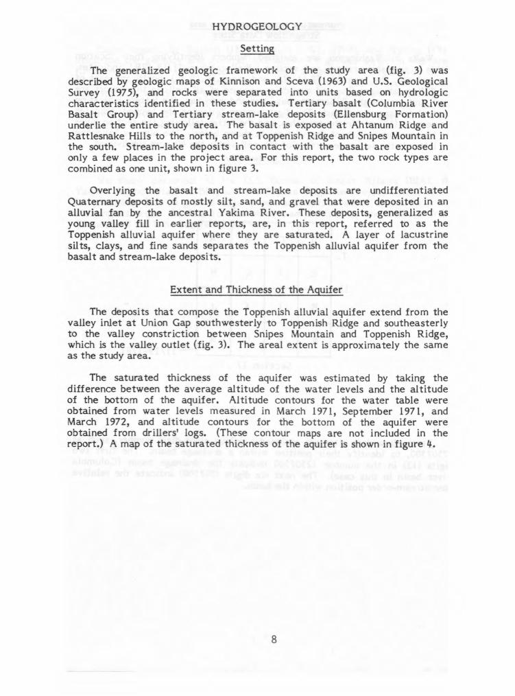
The generalized geologic framework of the study area (fig. 3) was described by geologic maps of Kinnison and Sceva (1963) and U.S. Geological Survey (1975), and rocks were separated into units based on hydrologic characteristics identified in these studies. Tertiary basalt (Columbia River Basalt Group) and Tertiary stream-lake deposits (Ellensburg Formation) underlie the entire study area. The basalt is exposed at Ahtanum Ridge and Rattlesnake Hills to the north, and at Toppenish Ridge and Snipes Mountain in the south. Stream-lake deposits in contact with the basalt are exposed in only a few places in the project area. For this report, the two rock types are combined as one unit, shown in figure 3.

Overlying the basalt and stream-lake deposits are undifferentiated Quaternary deposits of mostly silt, sand, and gravel that were deposited in an alluvial fan by the ancestral Yakima River. These deposits, generalized as young valley fill in earlier reports, are, in this report, referred to as the Toppenish alluvial aquifer where they are saturated. A layer of lacustrine silts, clays, and fine sands separates the Toppenish alluvial aquifer from the basalt and stream-lake deposits.

Extent and Thickness of the Aquifer

The deposits that compose the Toppenish alluvial aquifer extend from the valley inlet at Union Gap southwesterly to Toppenish Ridge and southeasterly to the valley constriction between Snipes Mountain and Toppenish Ridge, which is the valley outlet (fig. 3). The areal extent is approximately the same as the study area.

The saturated thickness of the aquifer was estimated by taking the difference between the average altitude of the water levels and the altitude of the bottom of the aquifer. Altitude contours for the water table were obtained from water levels measured in March 1971, September 1971, and March 1972, and altitude contours for the bottom of the aquifer were obtained from drillers' logs. (These contour maps are not included in the report.) A map of the saturated thickness of the aquifer is shown in figure 4.

8

Union Gap Rattlesnake

Ahtanum Ridge Hills

Uni 1 I

120°3500" Gap 120°22 30 EXPLANATION

46°30 00 ± Unconsolidated depoists of silt, sand, and gravel

— QUATERNARY

Basalt and partly consolidated stream-lake deposits (Includes — TERTIARY

Boundary of study area

Ellensburg Formation and Columbia River Basalt Group

fll Wapato

0 1 2 3 MILES

Harrah

1 I I I 1 1 I 1 1 2 3 4 KILOMETERS

Toppenish

Snipes Mountain

46°2000

7/Z8/ ce.14-

Geology modified from Toppenish Ridge Kinnison and Sceva (1963) and U.S. Geological Survey (1975)

FIGURE 3.--Generalized geology of the study area.

Union jot Gap it EXPLANATION

I o 120 35 00

46°30 00"d-

Boundary of study area

I

120°22 30 A B C

50-150 151-200 201-250

Saturated thickness, in feet

0

Observation well

0 1 2 3 MILES

I I '1 it 1 ' 0 1 2 3 4 KILOMETERS

FIGURE 4.--Saturated thickness used in the model of the Toppenish alluvial aquifer.

Precipitation

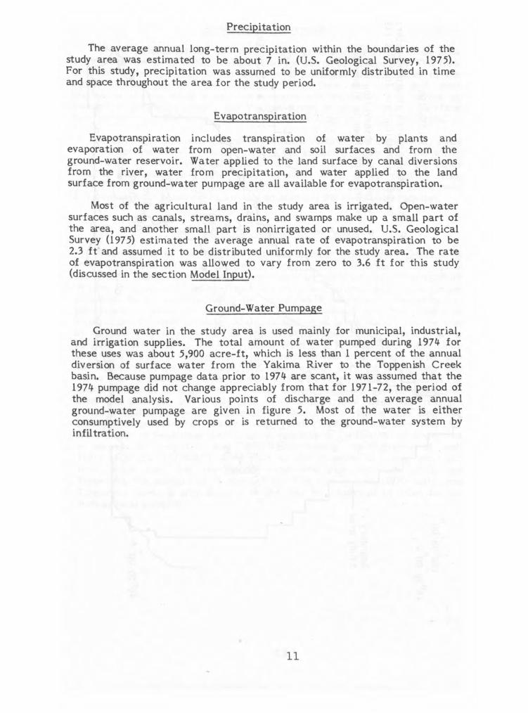
The average annual long-term precipitation within the boundaries of the study area was estimated to be about 7 in. (U.S. Geological Survey, 1975). For this study, precipitation was assumed to be uniformly distributed in time and space throughout the area for the study period.

Evapotranspiration

Evapotranspiration includes transpiration of water by plants and evaporation of water from open-water and soil surfaces and from the ground-water reservoir. Water applied to the land surface by canal diversions from the river, water from precipitation, and water applied to the land surface from ground-water pumpage are all available for evapotranspiration.

Most of the agricultural land in the study area is irrigated. Open-water surfaces such as canals, streams, drains, and swamps make up a small part of the area, and another small part is nonirrigated or unused. U.S. Geological Survey (1975) estimated the average annual rate of evapotranspiration to be 2.3 ft and assumed it to be distributed uniformly for the study area. The rate of evapotranspiration was allowed to vary from zero to 3.6 ft for this study (discussed in the section Model Input).

Ground-Water Pumpage

Ground water in the study area is used mainly for municipal, industrial, and irrigation supplies. The total amount of water pumped during 1974 for these uses was about 5,900 acre-ft, which is less than 1 percent of the annual diversion of surface water from the Yakima River to the Toppenish Creek basin. Because pumpage data prior to 1974 are scant, it was assumed that the 1974 pumpage did not change appreciably from that for 1971-72, the period of the model analysis. Various points of discharge and the average annual ground-water pumpage are given in figure 5. Most of the water is either consumptively used by crops or is returned to the ground-water system by infiltration.

Union lot. Gap ti-

I U 120°3500" 120°22 30

EXPLANATION 46°30 00 + 4

0.69 0 Well, major source of ground-water;

number is pumping rate in ft3/s (1974) 0.14 o 0

11/19-9K3 •

Water-level observation well, Boundary of 11/19-9K3 hydrograph shown in figure 6 study area 0.26

..•••••••=b• 0130 .13 fiN Wapato

0.13 0 00.13

0 1 2 3 MILES 00.13

I 1 1 i l I 1 00.13 0 1 2 3 4 KILOMETERS

3:t 11/19-36Q2 H arr, 0.26 0.43

0.5300 0.26 U r . 1.54 0.35 10/20-8C1 0 • 03 -84 0 64 o .

s Toppenish 00.i3

0/20-26H1

0.11 00.13 I 1 t 0

0.21 46°20 00 -i- H.-- 0 0.13 00.13 To ?l2..8/1

FIGURE 5.--Location of selected wells and rates of major ground-water pumpage.

Ground-Water Movement

The generalized lateral flow direction of ground water in the study area is shown by the water-table configuration for March 1972, figure 6. The flow direction is perpendicular to the water-level contours. Ground water in the aquifer enters laterally as subsurface flow from the north and west boundaries of the study area, moves south and southeast, and leaves as leakage to Toppenish Creek, the Yakima River, or drains, or as subsurface flow through the constriction between Toppenish Ridge and Snipes Mountain.

Locally, near streams, ground water has a vertical flow component, away from the stream where the water level in the stream is higher than the water level in the aquifer, and toward the stream from the aquifer where the water level in the aquifer is greater than the water level in the stream. Also, ground water moves vertically through the bottom of the aquifer where head differences occur between the alluvial aquifer and the lower basalt aquifer.

Water-Level Fluctuations in the Aquifer

Water levels in the Toppenish alluvial aquifer fluctuate in response to both natural and artificial changes in recharge and discharge. Responses to the natural changes are not as apparent as those to artificial changes, which include recharge from leaky irrigation canals and infiltration of land-applied irrigation water, and discharge by ground-water pumpage. The effect of ground-water pumpage on water levels is minimal, but the effect of infiltration of irrigation water is substantial. The latter effect can be seen by comparing hydrographs of four typical wells in the aquifer with a graph of irrigation diversions to the Main Canal from the Yakima River near Union Gap (figs. 5 and 7). These diversions, which provide most of the water used for irrigation in the study area, are about a mile south of Union Gap near where the Yakima River enters the project area. Each year, water levels rise in the aquifer as diversions to the canal system begin and decline when canal diversions decrease and finally stop. This intermittent stress has created a dynamic equilibrium where seasonal fluctuations are regular and long-term fluctuations are minimal. Water levels in well 11 /19-9K3 rise more than 15 ft from March to September each year in response to infiltration of water that is spread for irrigation and leaks from canals. Hydrographs of wells 11/19-36Q2 and 10/20-8C1 show that as the distance increases southward from Union Gap, the amount of water-level rise decreases until, near Toppenish, the annual rise is about 5 ft. The rise in well 10/20-26H1, near Toppenish Creek, is only about 2 ft and may he influenced by other factors, such as local pumping.

13

i on Gap it

120°35' 22'30" EXPLANATION 46°30'+

----750 Water-table contour, shows altitude of the water table in March 1972. Contour interval 10 feet; datum is NGVD of 1929. Arrows show

Boundary of general direction of ground-

study area water movement

0 Observation well

0 1 2 3 MILES

I I I 1 1 I I 0 1 2 3 4 KILOMETERS

120°10' 46°20'-f--

FIGURE 6.--Water-table configuration of the Toppenish

alluvial aquifer, March 1972.

14

V) I 140 [1111111111 I 1 I 1 i 1 I 1 1 1 1 LLJ 0 CC 1-1

120 V")

100 LLJ LL

80 o V)

60 VI

40 Li CD

1- 20 ,, LLJ <

0-4 LL- 0

5 11111

11/19-9K3 10

25

5

20

0

5 O

10 -

10/20-26H1 5 N„

111111 1 1 1 111iiillil11illti 10 --1

U F M A MU JASON DU F M A MJ JASONDJFM 1971 1972 1973

FIGURE 7.--Seasonal water-level changes in the Toppenish alluvial aquifer, and monthly diversions to the Main Canal from the Yakima River.

15

HYDRAULIC CHARACTERISTICS OF THE AQUIFER

In order to evaluate stresses on the ground-water-flow system, it is necessary to know the hydraulic characteristics of the aquifer - the lateral hydraulic conductivity, transmissivity, specific yield (storage coefficient), and the hydraulic connection between the aquifer and the major streams. Also, the vertical hydraulic conductivity of confining beds that underlie the alluvium is needed to estimate ground-water flow through the confining beds.

Lateral Hydraulic Conductivity

Lateral hydraulic conductivity was estimated primarily from specific-capacity data obtained from wells that were drilled by the BIA for a drought-relief program of the Wapato Irrigation Project. These data were supplemented with miscellaneous specific-capacity data from drillers' reports. Specific-capacity data could not be directly converted to transmissivity because nearly all wells in the area only partially penetrate the alluvial aquifer. Therefore, apparent values of transmissivity were calculated from the specific-capacity data using the method of Theis (in Bentall, 1963). The apparent values were divided by the length of well open to the aquifer to obtain an estimate of the lateral hydraulic conductivity of the aquifer, which provides the initial input for calibration of the digital model. A more rigorous analysis than this for estimating hydraulic conductivity is not warranted due to the lack of definitive well-test data. The distribution of estimated lateral hydraulic conductivity is shown in figure 8. Values of lateral hydraulic conductivity ranged from 0.009 ft/s near Wapato and in the area southeast of Toppenish to 0.0011 ft/s near the northwest and central parts of the study area. The variation is caused by the heterogeneity of the aquifer, as well as differences in well construction and results from well tests.

Vertical Hydraulic Conductivity of Confining Beds

Vertical hydraulic conductivity of the lacustrine silts, clays, and fine sands that underlie the alluvial aquifer was estimated, from earlier work by the U.S. Geological Survey (1975), to be about 1.0x10-7 ft/s. Water moves vertically through the clay beds, depending on the relative head differences between the aquifer above the clay beds and the aquifer below the beds. Data are not available to determine differences in vertical hydraulic conductivity that may or inay not exist within the clay beds, so the distribution was assumed (U.S. Geological Survey, 1975) to be a uniform value of 1.0x10-7 ft/s throughout the study area.

16

120°35'00" 120° ' " 2230 EXPLANATION

46°30 00 + -I-

B .0011-0030 .0031-0050

Boundary of D study area

0051-0070 .0071-0090

Lateral hydraulic conductivity in feet per second

0 1 2 3 MILES

I 1 1 1 1 1 1 0 1 2 3 4 KILOMETERS

FIGURE 8.--Lateral hydraulic conductivity used in the model.

Transmissivity and Specific Yield

Transmissivity was calculated as the product of saturated thickness and the lateral hydraulic conductivity of the aquifer. During model calibration (discussed in detail in the section Model Construction and Calibration), values of hydraulic conductivity at each node were adjusted until a statistical "best fit" between observed and calculated heads at 39 control wells was achieved. A map of transmissivity values computed during model calibration is shown in figure 9. Values of transmissivity range from about 5.0 ft2/s near Wapato and along Toppenish Creek to about 0.4 ft2 /s in the northwest and central parts of the area.

Specific yield of the aquifer was estimated to be 0.20 from earlier work by U.S. Geological Survey (1975) and was not adjusted for this study.

Aquifer-Stream Connection

The Toppenish alluvial aquifer is hydraulically connected to both the Yakima River and Toppenish Creek. The aquifer is also connected to the extensive system of irrigation canals and drains in the study area.

The aquifer gains considerable amounts of water from the Yakima River just downstream from Union Gap, according to Kinnison and Sceva (1963), and loses water to the river in the southeast part of the area. Data are not available to verify losses to or gains from the aquifer; however, they are estimated from the model in the section Transient Simulation. Data for Toppenish Creek are scant, but those that are available indicate that Toppenish Creek gains water from the aquifer through most of its reach as it flows through the study area. Data from two sites on Toppenish Creek, 12507000 and 12507500 (fig. 5), for the 1910 and 1911 water years show that the average monthly gain of Toppenish Creek between these two sites is about 106 ft3/s, with extremes ranging from 11 to 226 ft3/s. Stresses on the aquifer, in the form of irrigation diversion from the Main Canal, began in 1905, and it was assumed that these stresses were approximately the same for the study period.

The effect on ground-water levels of diverting and spreading irrigation water was shown earlier (fig. 7). In addition to the system of canals, a system of drains is intricately placed among the canals to alleviate saturated-soil conditions. These drains intercept the water table in much of the southern part of the area and generally flow throughout the year. They intercept the water table in the northern part when water levels rise as a result of recharge from excess irrigation water. The drains also collect runoff from excess irrigation water.

18

Union Gap

120°35'00" 120°22 30

46°30 00 + EXPLANATION

A B C

Boundary of 0.4-1.0 1.1-3.0 3.1-5.0 study area

Transmissivity, in square feet per second

0 1 2 3 MILES

1 I II I 1 0 1 2 3 4 KILOMETERS

46°20'00 f

FIGURE 9.--Transmissivity used in the model.

MODEL CONSTRUCTION AND CALIBRATION

A two-dimensional digital flow model, developed by the Geological Survey (Trescott and others, 1976), was used to simulate the movement of water in the Toppenish alluvial aquifer. Available data from well logs indicate an absence of vertical stratification in aquifer lithology, suggesting that the lateral and vertical hydraulic conductivity are about the same. Thus, vertical movement of water in the aquifer is insignificant except for some areas near streams and wells. For this reason, use of a two-dimensional model should introduce no serious error during simulation of lateral water movement in the aquifer. The model simulates ground-water flow by solving a set of linear equations derived for block-centered nodes on a finite-difference grid network. The overall grid for this study consists of 32 rows and 40 columns. There are 663 active nodes within the model boundaries (fig. 10).

Model Boundaries

The boundaries of the model, shown in figure 10, approximate the boundaries of the study area. The east boundary coincides with the Yakima River, and each node of this boundary was assigned a head value that was estimated from stream gages and topographic and average-water-level maps. Head values in these nodes were held constant during the time-averaged (steady-flow) aquifer simulation. The west boundary is the approximate contact between the alluvial aquifer and older valley-fill deposits. This boundary was treated partly as a no-flow boundary and partly as a constant-head boundary where heads were specified to simulate lateral movement of water from the older valley-fill deposits (U.S. Geological Survey, 1975), which are unaffected by stresses in the alluvial aquifer. The heads at nodes on the west boundary were determined from average water levels. The south boundary, which coincides with Toppenish Creek, is treated as a constant-head boundary similar to the east boundary. At the southeast corner, constant-flow values were specified for subsurface movement. The bottom of the aquifer is underlain by extensive clay beds, which were treated in the model as a leaky confining layer. With the exception of the west boundary, the constant-head boundaries were replaced with constant-flow boundaries during transient simulation. Additionally, canals and drains were simulated in the time-averaged model as areal recharge and discharge. During transient simulation the canals and drains were simulated using constant flow at the nodes where major diversions from canals or major flow accumulations to the drains occurred.

20

C

c 120°35' 22'30"

46°4_ C C 30' EXPLANATION

C 4 Model node (center of block) C A

C A A A Constant head nodes

Constant flow nodes C Canal

A C C C C C C C C

C A D Drain

C A A F Subsurface flow

Blank node on boundary indicates no flow

A C

rc C C A

C C C C D D 0 1 2 3 MILES C C C C C C C C C C C C C I 1

I 1

I 1 I

1

C 0 1 2 3 4 KILOMETERS

C D D A A

C 1

D A A

C C C C C C C C D A A

C D C C C C C C C C C C C C A A A

C D D

C C D D D D D D

C C C C C C C C C C C C C C C C C C C C C C D A

D A D D

U A

D D D D A A 120°10'

46° D 20'

A D D D D D D D

A A A A A A A A A A AA D

A A A A A A A A A A A A A A A F F F F

FIGURE 10.--Model grid network and boundary conditions used in the model.

Model Input

Input data to the model included precipitation, evapotranspiration, ground-water pumpage, confining-bed leakage, stream leakage, leakage from canals, and infiltration from excess irrigation water and discharge to drains. An average precipitation rate of 7 in./yr was used during simulation and was assumed to be uniformly distributed through all nodes of the model.

The evapotranspiration (ET) rate in the model was allowed to be a maximum of 3.6 ft/yr where the ground-water level was at the land surface and to decrease linearly as depth-to-water from land surface increased. The ET rate was zero whenever the depth-to-water exceeded 30 ft.

Pumpage from the alluvial aquifer is not a major stress on the aquifer. Much of the pumped water returns directly to the water table by infiltration. The total amount of pumpage for all uses averaged only about 8 ft3/s and was distributed through the study area as shown in figure 5.

The vertical hydraulic conductivity of confining beds was estimated to be 1.0x10-7ft/s. This, along with the heads on both top and bottom of the beds and the thickness of the beds, was used to calculate the leakage through the beds. The thickness of the beds ranges from about 50 ft in the southeast part of the area to about 100 ft in the northern part. During transient analysis, leakage from the confining bed itself was assumed to be negligible and, therefore, was not simulated in the model. All the data used for calculating the vertical leakage is given in U.S. Geological Survey (1975).

For the time-averaged model, specified heads at the boundary nodes associated with the Yakima River ranged from about 930 ft above sea level (NGVD) near Union Gap to about 690 ft near Snipes Mountain. Heads at nodes representing Toppenish Creek ranged from about 800 ft at the west boundary to about 700 ft near the southeast boundary. For the transient model, specified heads were replaced with specified flows that were calculated from the time-averaged model.

Subsurface outflow at the valley constriction near Snipes Mountain, estimated from earlier work (U. S. Geological Survey, 1975), was about 4 ft3/s and was distributed as constant flow through the nodes in the constriction.

22

The canal diversions were simulated in the time-averaged model using an average areal application rate of 4.45 ft/yr, which was computed from the annual diversion total. During transient simulation, only the large canals and laterals were represented in the model for simplicity. Each canal node shown in figure 10 represents constant flow for each time period in the transient model. Similarly, drains were simulated in the time-averaged model using an areal discharge rate of 2.40 ft/yr. During transient simulation, the nodes representing drains (fig. 10) were assigned constant flow for each time period.

Time-Averaged Simulation

Apparently, no long-term changes occur in water levels in the alluvial aquifer, as noted by U.S. Geological Survey (1975), indicating that recharge and discharge are in near equilibrium. This condition allowed for a time-averaged (quasi-steady-state) calibration of the model. The period from September 1971 to September 1972 was selected for calibration because of the availability of areally distributed water-level measurements in the aquifer.

The procedure for calibrating the time-averaged model was to adjust the initial values of hydraulic conductivity in the model until the least-average difference was obtained between the observed and calculated heads at 34 control wells (fig. 11). The smallest average head difference was about 4 ft, obtained by adjusting the initial estimates of hydraulic conductivity by a factor of 1.75. This factor includes adjustment for errors in initial lateral hydraulic conductivity or saturated thickness or a combination of both. The amount of error is unknown because wells in the aquifer are only partially penetrating, and the assumptions used for estimating hydraulic conductivity may differ from the actual flow system. The water budget calculated by the model is shown in table 1.

Only precipitation, canal and drain discharge, and pumpage in table 1 are known with reasonable accuracy. The model-computed values for the other budget items cannot be verified, but are probably reasonable because of the closeness of the fit between the observed and calculated heads (fig. 11). The budget provides an estimate of the amount of water gained and lost by the Yakima River and by Toppenish Creek. These data are used for input into the transient model, discussed next.

23

Vo

120°35' 46-30' + 920 ....----- 22'30"

+

EXPLANATION

____-- --- 800 Average water-level contour, 90 Sep. 1971-Mar. 1972. Contour

900-- 0

/ / 88C1

interval 20 feet; datum is NGVD of 1929

--- 800 Calculated water-level contour / 0 , — —

for time-averaged simulation

0 Water-level observation well

O , - a . Y) . . o - . ,',,t0

/ b .

0 1 2 3 MILES .."

../ . 1 1 1

1 1

1 1 1

840 — 5.— 0

0 1 2 3 4 KILOMTERS

/ /

0

/

46°201-1-

0 ,' /

/ C

CO N

120°10' +

FIGURE 11.--Average observed and model—calculated water—table configuration during 1971-72.

TABLE 1.--Water budget for the time-averaged simulation

(ft3/s)

Recharge

Precipitation-- 75 Subsurface inflow along west boundary 115 Leakage through bottom of aquifer 27 Leakage from Toppenish Creek 115 Leakage from Yakima River 194 Infiltration from irrigation water 571

Total 1,097

Discharge

Evapotranspiration 363 Leakage to Yakima River 105 Leakage to Toppenish Creek--- 254 Leakage through bottom of aquifer--- 54 Subsurface outflow along southeast boundary 4 Leakage to drains (Marion, Toppenish, and subdrain 35)- 308 Ground-water pumpage 8

Total-- ----- ----- ----- 1,096

25

Transient Simulation

The time-varying stresses on the Toppenish alluvial aquifer include precipitation, recharge from diversions to irrigation canals, evapotranspiration, discharge to drains, recharge and discharge to Toppenish Creek and the Yakima River, leakage through the bottom of the aquifer, and discharge by ground-water pumpage. For transient analysis, recharge from diversions to irrigation canals, evapotranspiration, discharge to drains, leakage through the bottom of the aquifer, and discharge by ground-water pumpage are allowed to vary with time. All other parameters remain constant for the simulation.

The response of the model to these time-varying stresses was simulated for the period March 1971 to March 1972. A 1-year period is sufficient to define the effect of stress on the aquifer because of the cyclic nature of water levels that, during each year, rise and decline to nearly the same levels (fig. 7). The 1-year simulation period was divided into two 6-month periods, April through September and October through March. These two periods correspond generally to the rise and decline of water levels in the aquifer during the year and to the irrigation and non-irrigation seasons.

The procedure for calibrating the transient model was to:

(a) initially estimate the amount of diverted irrigation water that recharges the aquifer and the amount of ground water discharged to drains;

(b) use the model to calculate the head in the aquifer at the end of a 6-month period;

(c) compare the calculated head with the observed head in the aquifer at that time;

(d) adjust values of drain discharge based on the above comparison; and

(e) repeat steps (b), (c), and (d) until the average difference between the model-calculated and the observed heads at 34 control wells reached a minimum.

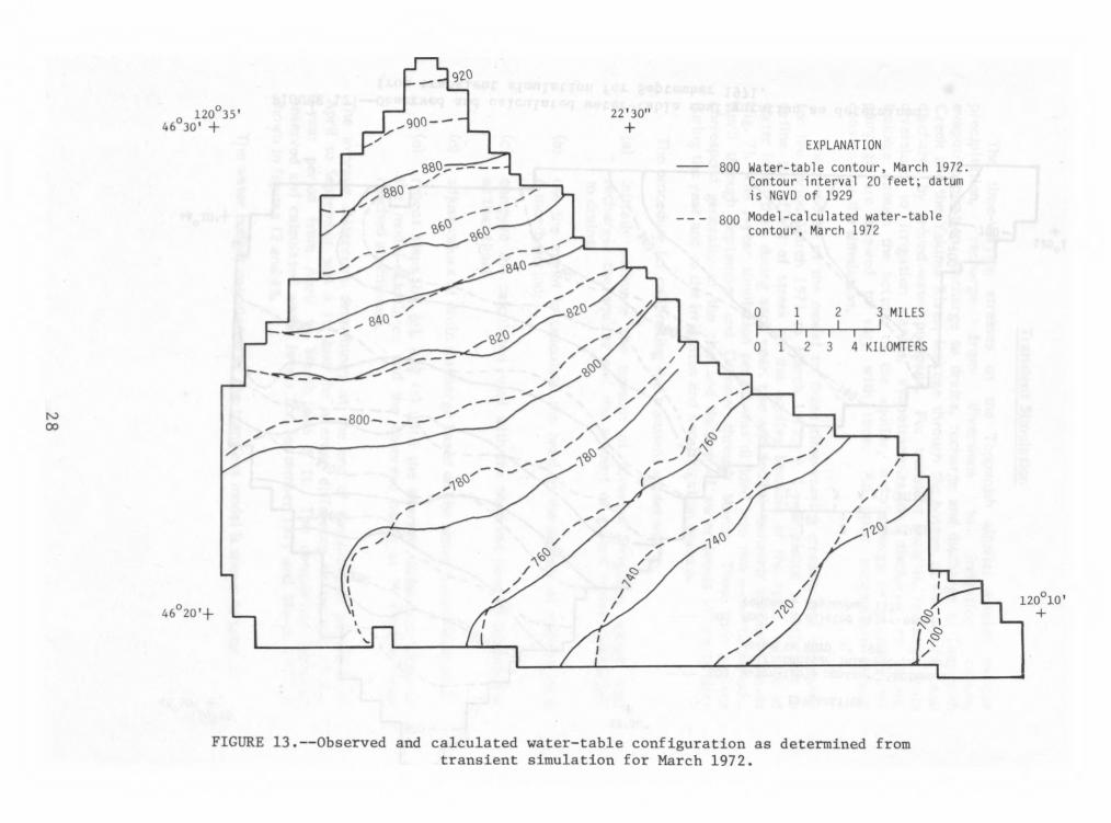
The average difference determined at the end of the 6-month period from April to September was 6 ft, and the average difference at the end of the 1-year period from April to March was 3 ft. The comparison between observed and calculated water levels for September 1971 and March 1972 is shown in figures 12 and 13.

The water budget calculated by the transient model is shown in table 2.

26

0120 35' 22'30" 46-30' +

EXPLANATION

800 Water-table contour, September 1971. Contour interval 20 feet; datum is NGVD of 1929

800 Model-calculated water-table contour, September 1971

B20, — 860 — 0 1 2 3 MILES

I I 1 I 1 1 I

1

0 1 2 3 4 KILOMTERS /

/

820 — — /

120°10' 46°20'+

FIGURE 12.--Observed and calculated water-table configuration as determined from transient simulation for September 1971.

9 "2

0 120°35' 46 30' d-

22'30"

EXPLANATION

----- 800 Water-table contour, March 1972. Contour interval 20 feet; datum is NGVD of 1929

— 800 Model-calculated water-table contour, March 1972

0

1 0

I 1

1 1

I 2

2 1

I 3

3 MILES

I 4 KILOMTERS

/

/ /

Qo /

/ -1(2.C)

46°20'A-

/

/ /

11' /

/

1

Y------ ol 0 1

,\ o o ,•\

120°10'

FIGURE 13.--Observed and calculated water-table configuration as determined from transient simulation for March 1972.

TABLE 2.--Water budget for the transient simulation

(ft3s)

Recharge

Precipitation 84 Subsurface inflow along west boundary 14 Leakage through bottom of aquifer 57 Leakage from Toppenish Creek 115 Leakage from Yakima River 194 Infiltration from irrigation water 637

Subtotal 1,101

Ground-water change in storage 65 Recharge and storage change - Total 1,166

Discharge

Evapotranspiration 379 Leakage to Yakima River 104 Leakage to Toppenish Creek 252 Leakage through bottom of aquifer 58 Subsurface outflow along southeast boundary 4 Leakage to drains (Marion, Toppenish, and subdrain 35)- 354 Ground-water pumpage 8

Total-- 1,159

29

Values in table 2 are averages for the 1-year simulation period. They were calculated by dividing the total volume of water accumulated for each budget item by the total time of simulation to obtain the volume-flow rate (ft3/s) or were taken from the time-averaged simulation, such as the values for Toppenish Creek and the Yakima River. The major difference between the time-averaged and transient budgets is the flow rate along the northwest boundary where constant heads were specified. The difference in flow rate along this boundary is due to a head gradient reversal during the period April to September, when application of irrigation water and subsequent ground-water recharge cause a rise in water levels in the aquifer (fig. 7). During this period, ground water discharges along the northwest boundary, but during the October to March period it recharges along this boundary. The net effect is a reduction in flow of about 100 ft3/s, as determined from the model analysis.

Other differences between the time-averaged and transient budgets for the items of precipitation, infiltration of irrigation water, and leakage to drains are caused by the representing of the Yakima River and Toppenish Creek in the time-averaged model as constant-head nodes. This method of simulation reduces the amount of area in the model that is affected by recharge and discharge.

Sensitivity

The time-averaged model was tested to see how changes in transmissivity affect the leakage to and from the Yakima River and Toppenish Creek. It was found that increasing or decreasing transmissivity by 30 percent increased or decreased, respectively, the net leakage to the Yakima River by about 15 ft3/s and to Toppenish Creek by about 40 ft3/s. The transient model was also tested using a 30-percent decrease and increase in transmissivity to show the effects of head change in the aquifer. A 30-percent decrease in transmissivity resulted in about a 1-ft increase in average head, and a 30-percent increase in transmissivity had only a negligible effect on average head in the aquifer.

30

MODEL UTILIZATION

The transient model was used to show the effect of increasing ground-water withdrawals on water levels in the Toppenish aquifer. A continuous ground-water pumping stress of 80 ft3/s (a tenfold increase above the 1974 pumping rates for the April to September period) was added to the model. Although a pumping rate of 80 ft3/s is somewhat an extreme condition, it demonstrated use of the model to predict aquifer heads. The areal distribution of water-level declines caused by the hypothetical pumping rate during the 6-month transient-simulation period is shown in figure 14.

The model, constructed and used as indicated above, will calculate the maximum values of water-level change in the aquifer under a given stress because the drains and streams are simulated as constant flow. Normally, when aquifer heads decline below the drain bottom, the flow to the drain stops. Also, when aquifer heads decline so as to increase the difference in head between the stream and aquifer, then streamflow depletion occurs. These constraints are not in the model, and, consequently, use of the model to calculate heads from a given stress results in maximum water-level changes. Thus, the calculated changes in water levels shown in figure 14 are greater than would be observed.

31

22'30" 120°35' 46°30' -I-

46°20'1-

EXPLANATION

A B

0-1 1-3 3-5

Water-level decline, in feet, due to hypothetical pumping stress

0

Well at which pumping stress was applied

0 1 2 3 MILES 1

!III 0 1 2 3 4 KILOMTERS

120°10'

FIGURE 14.--Distribution of water—level decline due to hypothetical pumping stress.

SUMMARY AND CONCLUSIONS

Annual diversions from Main Canal and Wanity Slough provide about 475,000 acre-ft of irrigation water to the study area. An additional 6,000 acre-ft per year are pumped from the alluvial aquifer. Th effect of ground-water pumpage on water levels is minimal, hut the effect of infiltration of irrigation water is substantial. Water levels rise about 15 ft from March to September in response to this infiltration.

A digital model was constructed and calibrated for the Toppenish alluvial aquifer to simulate movement of water in the alluvial aquifer. As determined during calibration of the model, the average difference between observed and model-calculated heads was about 4 ft. Results from the model show that the Yakima River losses an average of 90 ft3/s of water to the aquifer, and that Toppenish Creek gains an average of 137 ft3/s of water from the aquifer. No data are available for verification. The model was used to predict water-level drawdowns due to a hypothetical pumping stress. Because certain constraints are not included in the model, the calculated heads from a given stress result in greater water-level changes than would be observed.

RECOMMENDATIONS FOR FUTURE STUDIES

Because the Toppenish alluvial aquifer is hydraulically connected to the underlying basalts, and because management of the ground-water resource is an important consideration, future studies in this area would benefit from construction of an additional digital model that would incorporate both the alluvial aquifer and the underlying basalt aquifers. This more inclusive model would allow for better boundary definitions, and should take into account a variable stream-aquifer relationship.

This model would require additional data, including the simultaneous measurement of flow at various points on streams, canals, and drains and ground-water levels, in order to define the head-dependent stream-aquifer relationship.

33

REFERENCES

Bentall, Ray, 1963, Methods of determining permeability, transmis-sivity, and drawdown: U.S. Geological Survey Water-Supply Paper 1536-I, p. 332-336.

Kinnison, H. B., and Sceva, J. E., 1963, Effects of hydraulic and geologic factors on streamflow of the Yakima River basin, Washington: U.S. Geological Survey Water-Supply Paper 1595, 134 p.

Russell, I. C., 1893, A geological reconnaissance in central Washing-ton: U.S. Geological Survey Bulletin 108, 108 p.

Smith, G. 0., 1901, Geology and water resources of a portion of Yakima County, Washington: U.S. Geological Survey Water-Supply Paper 55, 68 p.

-----1903, Description of the Ellensburg quadrangle, Washington: U.S. Geological Survey Geologic Atlas, Folio 86, 7 p.

Trescott, P.C., Pinder, G. F., and Larson, S. P., 1976, Finite differ-ence model for aquifer simulation in two dimensions with results of numerical experiments: U.S. Geological Survey Techniques of Water-Resources Investigations, book 7, ch. Cl, 116 p.

U.S. Geological Survey, 1975, Water resources of the Toppenish Creek basin, Yakima Indian Reservation, Washington: U.S. Geological Survey Water-Resources Investigations 42-74, 144 p.

Waring, G. A., 1913, Geology and water resources of a portion of south-central Washington: U.S. Geological Survey Water-Supply Paper 316, 46 p.

34

1111111811000111111118