Deterministic Brownian Motion - McGill University

Deterministic Brownian Motion

Michael C. Mackey

September 4, 2014

Michael C. Mackey Deterministic Brownian Motion

Brownian Motion: Kappler, 1931

Figure: 30 minute record of mirror position at 760 mm Hg (upper) and4× 10−3 mm Hg (lower).


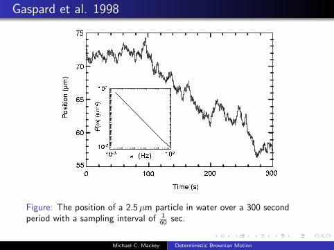
Gaspard et al. 1998

Figure: The position of a 2.5µm particle in water over a 300 secondperiod with a sampling interval of 1

60 sec.


Theoretical treatments of Brownian motion

Thorvald Thiele: 1880

Louis Bachelier: 1900 PhD thesis on stock and option markets

Albert Einstein: one of the amazing trio of 1905 papers

Marian Smoluchowski: 1906

Predictions of Einstein & Smoluchowski were verifiedexperimentally by Jean Perrin, 1908

Paul Levy

Paul Langevin

Norbert Wiener

And the list goes on. This field is now often referred to as thestudy of stochastic processes and is a mathematicallychallenging one.


Introduction

We are accustomed to ‘noise’ in our world and often invokestochastic processes to deal with this

Mathematicians have abstracted this into elaborate andbeautifully developed mathematics dealing with ‘random’events

While is clear that the assumption of ‘random’ events issufficient to explain aspects of data

It is by no means clear that it is necessary

Interesting Question: “Can one produce completelydeterministic theories that have the character of randomnessthat we see in the real world?”


Outline

The ‘usual’ Brownian Motion

Solution properties (numerical) of a differential delay equation

Quasi-Gaussian distributions

A deterministic quasi-Brownian motion

The filtered ‘random telegraph signal’

The mathematical problems preventing analytic proof

Conclusions and problems


Usual Brownian motion

dx

dt= v

mdv

dt= −γv + f (t)

f is a fluctuating “force” given by

f (t) = σξ(t)

ξ =dw

dt: a ‘white noise’ (delta correlated) which is the

‘derivative’ of a Wiener process w(t)

ξ(t): normally distributed with µ = 0, σ = 1


A differential delay equation: Lei & MCM, 2011

dx

dt= v

dv

dt= −γv + sin(2πβv(t − 1))

v(t) = φ(t), −1 ≤ t ≤ 0

The ‘random’ force is a rapidly oscillating function withrespect to v(t − 1)


Sample solution

0 20 40 60 80 100−0.5

0

0.5

t

v(t)

−0.2

0

0.2


Statistical quantifiers

Sampling: {vn}, where vn = v(n × 103∆t) and ∆t = 0.001

Mean: µ =1

N

∑Nn=1 vn

Bound: K = maxn |vn|

Standard deviation: σ =

√1

N

∑Nn=1(vn − µ)2

Excess kurtosis: γ2 =µ4σ4− 3 where µ4 =

1

N

∑Nn=1(vn − µ)4


Velocity statistics vs. β (γ = 1)

−1

0

1x 10

−3

(a)

μ

0.2

0.4

0.6(b)

K

0.1

0.3(c)

σ

10 20 30 40 50−1

−0.5

0

(d)

β

Exc

ess

Kur

tosi

s


Velocity statistics vs. γ (β = 20)

−4

−2

0

2x 10

−4

(a)

μ

0.1

0.2

0.3(b)

K

0.02

0.04

0.06

(c)

γ

σ

0 5 10 15 20 25 30−1.5

−1

−0.5

(d)

γ

Exc

ess

Kur

osis


Statistics: Dependence on β, γ from numerics

Bound

K (β, γ) =1

√γ(0.68

√β + 0.60

√γ)

Standard deviation

σ(β, γ) =0.32√βγ

Excess kurtosisγ2(β, γ) = −γ

β


Correlation function and times

0 10 200

0.5

1

1.5

2

β

Cor

rela

tion

time

(b)

0 10 200

0.2

0.4

0.6

0.8

1

(c)

γ

Cor

rela

tion

time

0 5 10

0

0.2

0.4

0.6

0.8

1

r

C(r

)

(a)

C (r) = limT→∞

∫ T0 v(t)v(t + r)dt∫ T

0 v(t)2dt' e−r/t0 ' e−γr


Quasi-Gaussian distributions

Quasi-Gaussian with µ = 0 and σ = 1 defined by

p(v ; 0, 1,K0) =

{Ce−v2/2, |v | ≤ K0

0, other wise

Normalize velocities to give

ζn =vn

σ(β, γ)

Sequence {ζn} has mean µ = 0, standard deviation σ = 1,and is bounded (numerically) by

K0 =K (β, γ)

σ(β, γ)'

√β/γ

0.21√β/γ + 0.19


Quasi-Gaussian simulations of v from DDE

0 10 20 30 40 502

2.5

3

3.5

4

4.5

5

β/γ

K0

(a)

−4 −2 0 2 40

0.1

0.2

0.3

0.4

0.5

v/σ

Den

sity

(b) β=2β=6β=8β=10


Deterministic Brownian Motion

Since numerically the velocity is like a ‘quasi-Gaussian noise’

now we construct a quasi-Brownian motion

using the full systemdx

dt= v

dv

dt= −γv + sin(2πβv(t − 1))


Deterministic BM simulations of x

0 2000 4000 6000 8000 10000−20

−10

0

10

20

30

t

x(t)

(a)

−10 −5 0 5 100

0.1

0.2

0.3

0.4

Δ x

Den

sity

(b) t=200

t=400t=600t=800


A differential nonlinearity delay equation

Replace the sin function with a piecewise constant nonlinearity:

dx

dt= v

dv

dt= −γv + 2

[H(sin(2πβv(t − 1))− 1

2)

]v(t) = φ(t), −1 ≤ t ≤ 0

H is the Heavyside step function

Now the ‘random’ force is discontinuous

Solutions are piecewise exponentials, increasing and decreasing

All of the statistical results are the same!

I think that the only really important thing is the rapidlyoscillating nature of the nonlinearity


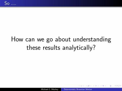
So ....

How can we go about understandingthese results analytically?


BM with ‘noise’ from a map: c.f. MCM & T-K (2006)

dx

dt= v

mdv

dt= −γv + f (t)

f (t) = mκ∑∞

n=0 ξ(t)δ(t − nτ),

ξ: a “highly chaotic” deterministic variable generated by

ξ(t) = T (ξ(t − τ)),

where T is an exact map or semi-dynamical system, e.g. thetent map on [−1, 1]

so the results of the simulation are (in principle) understoodanalytically since the numerical computations are replicating adiscrete time (high-dimensional) map

but we still can’t go to the continuous situation.


Random Telegraph Signal: Does this illuminate things?

Consider a signal ξ(t) that switches between +1 and −1’randomly’

+1 −→ −1 with transition probability kd∆t + o(∆t)

−1 −→ +1 with transition probability ku∆t + o(∆t)

This is the random telegraph signal

Fully characterized analytically


Linear dichotomous flow (LDF)

dv

dt= −γv + ξ

The ‘random’ force ξ is the random telegraph signal

Pick kd = ku ≡ αSolutions are continuous and consist of segments that arepiecewise exponentials, increasing and decreasing

State space is V =

(−1

γ,

1

γ

)Stationary density is

p∗(x) =γ

B(12 ,

αγ

) (1− γ2x2)α/γ−1 → 1√2πσ

e−x2/2σ2

,α

γ→∞


DDE versus LDF results

Compare numerical DDE results with the LDF results

Quantity DDE (numerical) LDF (exact)

Bound ∼ ±(√βγ + γ)−1 ±γ−1

Correlation ∼ e−γt e−γt

Mean µ ∼ 0 0

SD σ ∼ (βγ)−1/2 (αγ)−1/2

Kurtosis γ2 ∼ −γ/β −γ/αI think the result in red for the DDE is due to numerics

If β ≡ α then the exact results for the linear dichotomous flowmatch the numerical results from the differential delayequation


Density evolution: ODE’s

Ifdxidt

= Fi (x) i = 1, . . . , d ,

the evolution of f (t, x) ≡ Pt f0(x) is governed by the generalizedLiouville equation:

∂f

∂t= −

∑i

∂(f Fi )

∂xi


Density evolution in stochastic systems

For stochastic differential equations

dxidt

= Fi (x) + σ(x)ξi , i = 1, . . . , d

f (t, x) ≡ Pt f0(x) satisfies the Fokker-Planck equation:

∂f

∂t= −

∑i

∂(f Fi )

∂xi+

1

2

∑i ,j

∂2(σ2f )

∂xi∂xj


Stationary densities

A density f∗ such that PtS f∗ = f∗ is a stationary density (fixed

point) of PS

For the system of ordinary differentialequations, f∗ is given by the solution of∑

i

∂(f∗Fi )

∂xi= 0,

For a system of stochastic differential equations, f∗ is thesolution of

−∑i

∂(f∗Fi )

∂xi+

1

2

∑i ,j

∂2(σ2f∗)

∂xi∂xj= 0.


The problem with DDE’s & density evolution

If x evolves under the action of dynamics described by adifferential delay equation (DDE)

dx(t)

dt= F(x(t), xτ (t)), xτ (t) ≡ x(t − τ)

then we would like to know how some “density” of thevariable x will evolve in time

We would like to be able to write down an equation like

UNKNOWN OPERATOR (DENSITY) = 0

Unfortunately we don’t know how to do this

Why?


Formal ‘Transfer operator’

dx(t)

dt= F(x(t), xτ (t)), x(t ′) ≡ φ(t ′)∀t ′ ∈ [−τ, 0]

induces a flow Tt on a

phase space of continuous functions C = C ([−τ, 0],R)

{Tt : t ≥ 0} : C → C is a strongly continuous semigroup


Formal ‘Transfer operator’

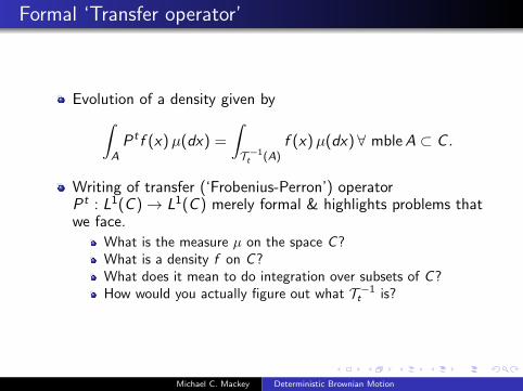
Evolution of a density given by∫APt f (x)µ(dx) =

∫T −1t (A)

f (x)µ(dx) ∀ mbleA ⊂ C .

Writing of transfer (‘Frobenius-Perron’) operatorPt : L1(C )→ L1(C ) merely formal & highlights problems thatwe face.

What is the measure µ on the space C?What is a density f on C?What does it mean to do integration over subsets of C?How would you actually figure out what T −1

t is?


Densities and DDE’s: The basic problem

Differential delay equations–infinite dimensional systems

Must specify an initial function on an interval [−τ, 0]

dx(t)

dt= F(x(t), xτ (t)), x(t ′) ≡ φ(t ′)∀t ′ ∈ [−τ, 0]

How to define a density in an infinite dimensional space?

If we can figure out how to define a density on this space

how can we relate it to what we actually measure in thelaboratory?


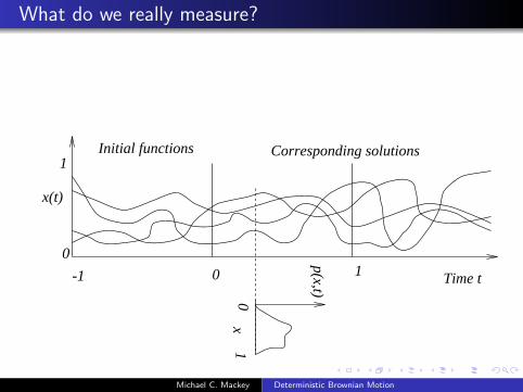
What do we really measure?

0

1

Time t-1 0 1

Initial functions Corresponding solutions

x0

1

x(t)p(x,t)


Conclusions

From numerical experiments it appears that one can producea quasi-random process with deterministic dynamics

The numerical DDE results match the analytic predictions fora filtered random telegraph signal

However, confirmation awaits a formal proof and the problemsinvolved are legion

If true, it is no longer necessary to postulate random processesto explain ‘noise’ in data

The results suggest that all events in the natural world can beexplained using completely deterministic dynamics (i.e.deterministic dynamics are sufficient)

Implications for the interpretation of quantum mechanics and“free will” (but that is another talk–probably over a coldbeer!)


Thanks to Jinzhi Lei (Beijing)


and Marta Tyran (Katowice)


Research supported by

NSERC, MITACS, and Alexander von Humboldt Stiftung

Zhou Pei-Yuan Center for Applied Mathematics (TsinghuaUniversity, Beijing)

Polish State Committee for Scientific Research


References

J. Lei & M.C. Mackey. “Deterministic Brownian motiongenerated from differential delay equations”, Phys. Rev. E(2011) 84, 041105-1-14

M.C. Mackey & M. Tyran-Kaminska. “DeterministicBrownian Motion: The effects of perturbing a dynamicalsystem by a chaotic semi-dynamical system”, Phys. Reports(2006) 422, 167-222


Deterministic Brownian Motion - McGill University

Documents

Transcript of Deterministic Brownian Motion - McGill University