Introduction to path integrals - McGill Physicshilke/719.pdf1 Introduction to path integrals v....
64
1 Introduction to path integrals v. January 22, 2006 Phys 719 - M. Hilke CONTENT • Classical stochastic dynamics • Brownian motion (random walk) • Quantum dynamics • Free particle • Particle in a potential • Driven harmonic oscillator • Semiclassical approximation • Statistical description (imaginary time) • Quantum dissipative systems INTRODUCTION Path integrals are used in a variety of fields, including stochastic dynamics, polymer physics, protein folding, field theories, quantum mechanics, quantum field theo- ries, quantum gravity and string theory. The basic idea is to sum up all contributing paths. Here we will overview the technique be starting on classical dynamics, in par- ticular, the random walk problem before we discuss the quantum case by looking at a particle in a potential, and finish with an example of a quantum dissipative system, where this technique bares all its fruits. CLASSICAL STOCHASTIC DYNAMICS The classical equation of motion for a particle in a fluctuating environment is simply given by m dv dt = F (t) - v/B (1) where m is the mass, v the velocity and B describes the friction of the particle. This equation is the Langevin equation if F (t) is a fluctuating force. These equa- tions are often difficult to solve and one possibility is to look at the probability density ρ(x, t) instead. This approach leads to expressing ρ in terms of a master- equation (Fokker-Planck) which takes on the following form: ∂ρ ∂t = - ∂ ∂x (μ 1 ρ)+ ∂ 2 ∂x 2 (μ 2 ρ) (2) with μ 1 (x) and μ 2 (x) the first and second moments of the transition probabilities. Another approach is to use path integrals. We will use the example of a simple brownian motion (the random walk) to illustrate the concept of the path integral (or Wiener integral) in this context. DISCRETE RANDOM WALK The discrete random walk describes a particle (or per- son) moving along fixed segments for fixed time intervals (of unit 1). The choice of direction for each new segment is random. We will assume that only perpendicular di- rection are possible (4 possibilities in 2D and 6 in 3D). The important quantity is the probability to reach x at time t, when the random walker started at x 0 at time t 0 : P (x, t; x 0 ,t 0 ). (3) For this probability the following normalization condi- tions apply: P (x, t; x 0 ,t)= δ x,x 0 and for (t>t 0 ) X x P (x, t; x 0 ,t 0 )=1. (4) This leads to P (x, t + 1; x 0 ,t 0 )= 1 2D X hξi P (ξ,t; x 0 ,t 0 ), (5) where hξ i represent the nearest neighbors of x. This is solved by the Fourier transform: P (x, t, x 0 ,t 0 )= Z π -π d D k (2π) D e ikx ˜ P (k,t), (6) which leads to ˜ P (k,t+1) = 1 D D X μ=1 cos(k μ ) ˜ P (k,t) with ˜ P (k,t 0 )= e -ikx 0 . (7) Hence, P (x, t; x 0 ,t 0 )= Z π -π d D k (2π) D e ik(x-x 0 ) ˆ 1 D D X μ=1 cos(k μ ) ! t-t 0 , (8) where we used 7 iteratively. Now, instead of using the probability we introduce the probability density p = P/a D , where a ia the step size, which will allow us to take the limit a → 0, for the continuous case with the variable change (k → ak, x → x/a). Hence,
Transcript of Introduction to path integrals - McGill Physicshilke/719.pdf1 Introduction to path integrals v....
1
Introduction to path integrals
v. January 22, 2006Phys 719 - M. Hilke
CONTENT
• Classical stochastic dynamics
• Brownian motion (random walk)
• Quantum dynamics
• Free particle
• Particle in a potential
• Driven harmonic oscillator
• Semiclassical approximation
• Statistical description (imaginary time)
• Quantum dissipative systems
INTRODUCTION
Path integrals are used in a variety of fields, includingstochastic dynamics, polymer physics, protein folding,field theories, quantum mechanics, quantum field theo-ries, quantum gravity and string theory. The basic ideais to sum up all contributing paths. Here we will overviewthe technique be starting on classical dynamics, in par-ticular, the random walk problem before we discuss thequantum case by looking at a particle in a potential, andfinish with an example of a quantum dissipative system,where this technique bares all its fruits.
CLASSICAL STOCHASTIC DYNAMICS
The classical equation of motion for a particle in afluctuating environment is simply given by
mdv
dt= F (t)− v/B (1)
where m is the mass, v the velocity and B describes thefriction of the particle. This equation is the Langevinequation if F (t) is a fluctuating force. These equa-tions are often difficult to solve and one possibility isto look at the probability density ρ(x, t) instead. Thisapproach leads to expressing ρ in terms of a master-equation (Fokker-Planck) which takes on the followingform:
∂ρ
∂t= − ∂
∂x(µ1ρ) +
∂2
∂x2(µ2ρ) (2)
with µ1(x) and µ2(x) the first and second moments ofthe transition probabilities.
Another approach is to use path integrals. We will usethe example of a simple brownian motion (the randomwalk) to illustrate the concept of the path integral (orWiener integral) in this context.
DISCRETE RANDOM WALK
The discrete random walk describes a particle (or per-son) moving along fixed segments for fixed time intervals(of unit 1). The choice of direction for each new segmentis random. We will assume that only perpendicular di-rection are possible (4 possibilities in 2D and 6 in 3D).The important quantity is the probability to reach x attime t, when the random walker started at x′ at time t′:
P (x, t; x′, t′). (3)
For this probability the following normalization condi-tions apply:
P (x, t; x′, t) = δx,x′ and for (t > t′)∑
x
P (x, t;x′, t′) = 1.
(4)This leads to
P (x, t + 1; x′, t′) =1
2D
∑
〈ξ〉P (ξ, t; x′, t′), (5)
where 〈ξ〉 represent the nearest neighbors of x. This issolved by the Fourier transform:
P (x, t, x′, t′) =∫ π
−π
dDk
(2π)DeikxP (k, t), (6)
which leads to
P (k, t+1) =1D
D∑µ=1
cos(kµ)P (k, t) with P (k, t′) = e−ikx′ .
(7)Hence,
P (x, t; x′, t′) =∫ π
−π
dDk
(2π)Deik(x−x′)
(1D
D∑µ=1
cos(kµ)
)t−t′
,
(8)where we used 7 iteratively. Now, instead of using theprobability we introduce the probability density p =P/aD, where a ia the step size, which will allow us totake the limit a → 0, for the continuous case with thevariable change (k → ak, x → x/a). Hence,

2
p(x, t;x′, 0) =∫ ∞
−∞
dDk
(2π)Deik(x−x′)
(1D
D∑µ=1
cos(akµ)
)(t−t′)2D/a2
︸ ︷︷ ︸'e−tk2
, (9)
where we used 1D
∑Dµ=1 cos(akµ) ' (1− a2k2/2D + · · · ).
Hence,
p(x, t; x′, 0) =∫ ∞
−∞
dDk
(2π)Deik(x−x′)−tk2
=1
4πtD/2e−
(x−x′)24t , (10)
which is the standard diffusion equation. The normaliza-tion of the probability density requires
∫dDxp(x, t; x′, t′) = 1 (11)
and
limt→0
p(x, t;x′, t′) = δD(x− x′) (12)
. It is now possible to describe the evolution from aninitial point (xi, 0) to a final point (xf , t) by inserting anintermediate point (x1, t1) and integrating over it, i.e.,
p(xf , t; xi, 0) =∫
dDx1p(xf , t;x1, t1)p(x1, t1; xi, 0) (0 < t1 < tf ).
(13)We can perform a similar decomposition for n interme-diate points, with xf = xn and x0 = xi. This then leadsto the summation over n paths, which is the mainidea of the path integral. Thus, using (13) and (10) weobtain
p(xf , t; xi, 0) =∫ n−1∏
j=1
dDxj
4π(tj+1 − tj)D/2
1
4πtD/21
e− 1
4
Pn−1j=0
(xj+1−xj)2
tj+1−tj . (14)
Since
n−1∑
j=0
(xj+1 − xj)2
tj+1 − tj=
∫ t
0
dsx2, (15)
we define the path integral as
p(xf , t; xi, 0) =∫ xf
xi
Dx(s)e−14
R t0 dsx2
. (16)
Here D denotes the multiple integrals defined in (14) andrepresents the sum over all paths (Wiener integral). Wewill see in the next sections that a very similar expressionexists in quantum mechanics. In classical systems thispath integral is useful when there exist many ways to getform one point to the other (like in stochastic processes)and where it is then necessary to sum over all possiblepaths.

Quantum Mechanics
Feynman Path Integral
⇒
⇒
with
Splitting the time evolution in 2:
⇒
Written in eigenfunction basis: ⇒
Hilke
(For details see appended notes by G.L. Ingold)
Free particle: ⇒
using
and
⇒
In terms of the classical action: (classical free path)
⇒
⇒
Particle in a potential:
using
and
⇒
{
0
⇒

c
The Feynman path integral
Driven harmonic oscillator:
= Classical path+quantum fluctuationsfluctuations
Classical path
⇓
with
;
Hence,
Normalization:
but
and
⇒
Semiclassical approximation:
0
⇒
with⇒
Imaginary time (statistical properties):
where
But
is the quantum
partition function
Shows that for
hence
with
The equilibrium density operator:
Applying this to the harmonic oscillator:
Dissipative Systems:
{
Effective action:(the density matrix)
(initially independent)
(tracing out the environment)
(tracing out the environment)

⇒
Path Integrals and Their Application to
Dissipative Quantum Systems
Gert-Ludwig Ingold
Institut fur Physik, Universitat Augsburg, D-86135 Augsburg
to be published in “Coherent Evolution in Noisy Environments”,Lecture Notes in Physics, http://link.springer.de/series/lnpp/
c© Springer Verlag, Berlin-Heidelberg-New York

Path Integrals and Their Application to
Dissipative Quantum Systems
Gert-Ludwig Ingold
Institut fur Physik, Universitat Augsburg, D-86135 Augsburg, Germany
1 Introduction
The coupling of a system to its environment is a recurrent subject in this collec-tion of lecture notes. The consequences of such a coupling are threefold. First ofall, energy may irreversibly be transferred from the system to the environmentthereby giving rise to the phenomenon of dissipation. In addition, the fluctuatingforce exerted by the environment on the system causes fluctuations of the systemdegree of freedom which manifest itself for example as Brownian motion. Whilethese two effects occur both for classical as well as quantum systems, there existsa third phenomenon which is specific to the quantum world. As a consequenceof the entanglement between system and environmental degrees of freedom acoherent superposition of quantum states may be destroyed in a process referredto as decoherence. This effect is of major concern if one wants to implement aquantum computer. Therefore, decoherence is discussed in detail in Chap. 5.
Quantum computation, however, is by no means the only topic where thecoupling to an environment is relevant. In fact, virtually no real system can beconsidered as completely isolated from its surroundings. Therefore, the phenom-ena listed in the previous paragraph play a role in many areas of physics andchemistry and a series of methods has been developed to address this situation.Some approaches like the master equations discussed in Chap. 2 are particularlywell suited if the coupling to the environment is weak, a situation desired inquantum computing. On the other hand, in many solid state systems, the envi-ronmental coupling can be so strong that weak coupling theories are no longervalid. This is the regime where the path integral approach has proven to be veryuseful.
It would be beyond the scope of this chapter even to attempt to give a com-plete overview of the use of path integrals in the description of dissipative quan-tum systems. In particular for a two-level system coupled to harmonic oscillatordegrees of freedom, the so-called spin-boson model, quite a number of approx-imations have been developed which are useful in their respective parameterregimes. This chapter rather attempts to give an introduction to path integralsfor readers unfamiliar with but interested in this method and its application todissipative quantum systems.
In this spirit, Sect. 2 gives an introduction to path integrals. Some aspectsdiscussed in this section are not necessarily closely related to the problem ofdissipative systems. They rather serve to illustrate the path integral approachand to convey to the reader the beauty and power of this approach. In Sect. 3
2 Gert-Ludwig Ingold
we elaborate on the general idea of the coupling of a system to an environment.The path integral formalism is employed to eliminate the environmental degreesof freedom and thus to obtain an effective description of the system degree offreedom. The results provide the basis for a discussion of the damped harmonicoscillator in Sect. 4. Starting from the partition function we will examine severalaspects of this dissipative quantum system.
Readers interested in a more in-depth treatment of the subject of quantumdissipation are referred to existing textbooks. In particular, we recommend thebook by U. Weiss [1] which provides an extensive presentation of this topictogether with a comprehensive list of references. Chapter 4 of [2] may serve as amore concise introduction complementary to the present chapter. Path integralsare discussed in a whole variety of textbooks with an emphasis either on thephysical or the mathematical aspects. We only mention the book by H. Kleinert[3] which gives a detailed discussion of path integrals and their applications indifferent areas.
2 Path Integrals
2.1 Introduction
The most often used and taught approach to nonrelativistic quantum mechan-ics is based on the Schrodinger equation which possesses strong ties with thethe Hamiltonian formulation of classical mechanics. The nonvanishing Poissonbrackets between position and momentum in classical mechanics lead us to in-troduce noncommuting operators in quantum mechanics. The Hamilton functionturns into the Hamilton operator, the central object in the Schrodinger equation.One of the most important tasks is to find the eigenfunctions of the Hamiltonoperator and the associated eigenvalues. Decomposition of a state into theseeigenfunctions then allows us to determine its time evolution.
As an alternative, there exists a formulation of quantum mechanics basedon the Lagrange formalism of classical mechanics with the action as the cen-tral concept. This approach, which was developed by Feynman in the 1940’s[4,5], avoids the use of operators though this does not necessarily mean that thesolution of quantum mechanical problems becomes simpler. Instead of findingeigenfunctions of a Hamiltonian one now has to evaluate a functional integralwhich directly yields the propagator required to determine the dynamics of aquantum system. Since the relation between Feynman’s formulation and classi-cal mechanics is very close, the path integral formalism often has the importantadvantage of providing a much more intuitive approach as we will try to conveyto the reader in the following sections.
2.2 Propagator
In quantum mechanics, one often needs to determine the solution |ψ(t)〉 of thetime-dependent Schrodinger equation
i~∂|ψ〉∂t
= H |ψ〉 , (1)
Path Integrals and Quantum Dissipation 3
where H is the Hamiltonian describing the system. Formally, the solution of (1)may be written as
|ψ(t)〉 = T exp
(
− i
~
∫ t
0
dt′H(t′)
)
|ψ(0)〉 . (2)
Here, the time ordering operator T is required because the operators correspond-ing to the Hamiltonian at different times in general due not commute. In thefollowing, we will restrict ourselves to time-independent Hamiltonians where (2)simplifies to
|ψ(t)〉 = exp
(
− i
~Ht
)
|ψ(0)〉 . (3)
As the inspection of (2) and (3) demonstrates, the solution of the time-dependentSchrodinger equation contains two parts: the initial state |ψ(0)〉 which serves asan initial condition and the so-called propagator, an operator which contains allinformation required to determine the time evolution of the system.
Writing (3) in position representation one finds
〈x|ψ(t)〉 =
∫
dx′〈x| exp
(
− i
~Ht
)
|x′〉〈x′|ψ(0)〉 (4)
or
ψ(x, t) =
∫
dx′K(x, t, x′, 0)ψ(x′, 0) (5)
with the propagator
K(x, t, x′, 0) = 〈x| exp
(
− i
~Ht
)
|x′〉 . (6)
It is precisely this propagator which is the central object of Feynman’s formu-lation of quantum mechanics. Before discussing the path integral representationof the propagator, it is therefore useful to take a look at some properties of thepropagator.
Instead of performing the time evolution of the state |ψ(0)〉 into |ψ(t)〉 in onestep as was done in equation (3), one could envisage to perform this procedurein two steps by first propagating the initial state |ψ(0)〉 up to an intermediatetime t1 and taking the new state |ψ(t1)〉 as initial state for a propagation overthe time t− t1. This amounts to replacing (3) by
|ψ(t)〉 = exp
(
− i
~H(t− t1)
)
exp
(
− i
~Ht1
)
|ψ(0)〉 (7)
or equivalently
ψ(x, t) =
∫
dx′∫
dx′′K(x, t, x′′, t1)K(x′′, t1, x′, 0)ψ(x′, 0) . (8)
Comparing (5) and (8), we find the semigroup property of the propagator
K(x, t, x′, 0) =
∫
dx′′K(x, t, x′′, t1)K(x′′, t1, x′, 0) . (9)
4 Gert-Ludwig Ingold
0 t1 t
x′
x
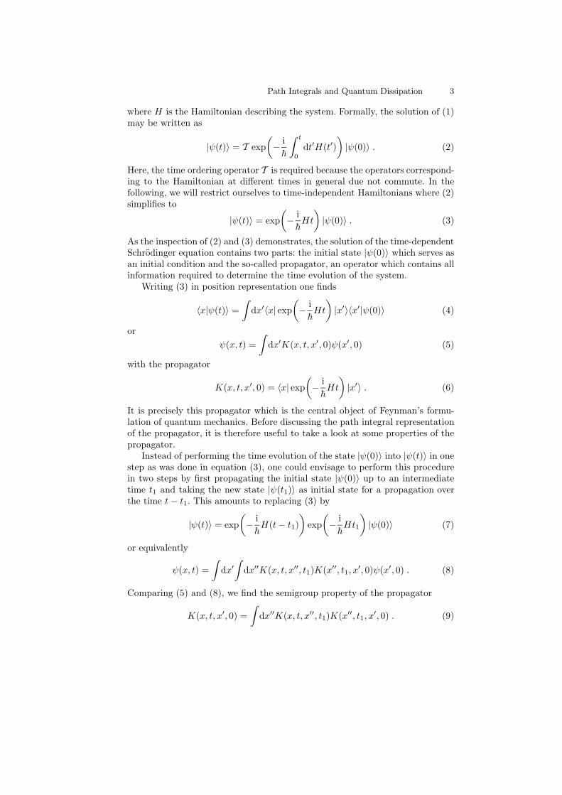
Fig. 1. According to the semigroup property (9) the propagator K(x, t, x′, 0) may bedecomposed into propagators arriving at some time t1 at an intermediate point x′′ andpropagators continuing from there to the final point x
This result is visualized in Fig. 1 where the propagators between space-timepoints are depicted by straight lines connecting the corresponding two points.At the intermediate time t1 one has to integrate over all positions x′′. This insightwill be of use when we discuss the path integral representation of the propagatorlater on.
The propagator contains the complete information about the eigenenergiesEn and the corresponding eigenstates |n〉. Making use of the completeness of theeigenstates, one finds from (6)
K(x, t, x′, 0) =∑
n
exp
(
− i
~Ent
)
ψn(x)ψn(x′)∗ . (10)
Here, the star denotes complex conjugation. Not only does the propagator con-tain the eigenenergies and eigenstates, this information may also be extractedfrom it. To this end, we introduce the retarded Green function
Gr(x, t, x′, 0) = K(x, t, x′, 0)Θ(t) (11)
where Θ(t) is the Heaviside function which equals 1 for positive argument t andis zero otherwise. Performing a Fourier transformation, one ends up with thespectral representation
Gr(x, x′, E) = − i
~
∫ ∞
0
dt exp
(
i
~Et
)
Gr(t)
=∑
n
ψn(x)ψn(x′)∗
E − En + iε,
(12)
where ε is an infinitely small positive quantity. According to (12), the poles ofthe energy-dependent retarded Green function indicate the eigenenergies whilethe corresponding residua can be factorized into the eigenfunctions at positionsx and x′.
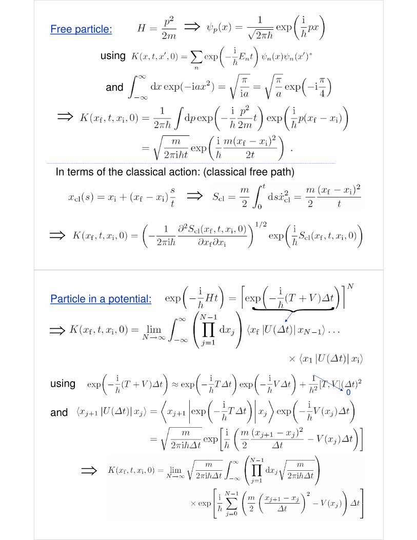
2.3 Free Particle
An important step towards the path integral formulation of quantum mechanicscan be made by considering the propagator of a free particle of mass m. The
Path Integrals and Quantum Dissipation 5
eigenstates of the corresponding Hamiltonian
H =p2
2m(13)
are momentum eigenstates
ψp(x) =1√2π~
exp
(
i
~px
)
(14)
with a momentum eigenvalue p out of a continuous spectrum. Inserting theseeigenstates into the representation (10) of the propagator, one finds by virtue of
∫ ∞
−∞
dx exp(−iax2) =
√
π
ia=
√
π
aexp(
−iπ
4
)
(15)
for the propagator of the free particle the result
K(xf , t, xi, 0) =1
2π~
∫
dp exp
(
− i
~
p2
2mt
)
exp
(
i
~p(xf − xi)
)
=
√
m
2πi~texp
(
i
~
m(xf − xi)2
2t
)
.
(16)
It was already noted by Dirac [6] that the quantum mechanical propagatorand the classical properties of a free particle are closely related. In order todemonstrate this, we evaluate the action of a particle moving from xi to xf intime t. From the classical path
xcl(s) = xi + (xf − xi)s
t(17)
obeying the boundary conditions xcl(0) = xi and xcl(t) = xf , the correspondingclassical action is found as
Scl =m
2
∫ t
0
dsx2cl =
m
2
(xf − xi)2
t. (18)
This result enables us to express the propagator of a free particle entirely interms of the classical action as
K(xf , t, xi, 0) =
(
− 1
2πi~
∂2Scl(xf , t, xi, 0)
∂xf∂xi
)1/2
exp
(
i
~Scl(xf , t, xi, 0)
)
. (19)
This result is quite remarkable and one might suspect that it is due to a pecu-liarity of the free particle. However, since the propagation in a general potential(in the absence of delta function contributions) may be decomposed into a seriesof short-time propagations of a free particle, the result (19) may indeed be em-ployed to construct a representation of the propagator where the classical actionappears in the exponent. In the prefactor, the action appears in the form shownin equation (19) only within the semiclassical approximation (cf. Sect. 2.8) orfor potentials where this approximation turns out to be exact.
6 Gert-Ludwig Ingold
2.4 Path Integral Representation of Quantum Mechanics
While avoiding to go too deeply into the mathematical details, we neverthelesswant to sketch the derivation of the path integral representation of the propaga-tor. The main idea is to decompose the time evolution over a finite time t intoN slices of short time intervals ∆t = t/N where we will eventually take the limitN → ∞. Denoting the operator of the kinetic and potential energy by T and V ,respectively, we thus find
exp
(
− i
~Ht
)
=
[
exp
(
− i
~(T + V )∆t
)]N
. (20)
For simplicity, we will assume that the Hamiltonian is time-independent eventhough the following derivation may be generalized to the time-dependent case.We now would like to decompose the short-time propagator in (20) into a partdepending on the kinetic energy and another part containing the potential en-ergy. However, since the two operators do not commute, we have to exercisesome caution. From an expansion of the Baker-Hausdorff formula one finds
exp
(
− i
~(T + V )∆t
)
≈ exp
(
− i
~T∆t
)
exp
(
− i
~V ∆t
)
+1
~2[T, V ](∆t)2 (21)
where terms of order (∆t)3 and higher have been neglected. Since we are inter-ested in the limit ∆t → 0, we may neglect the contribution of the commutatorand arrive at the Trotter formula
exp
(
− i
~(T + V )t
)
= limN→∞
[U(∆t)]N
(22)
with the short time evolution operator
U(∆t) = exp
(
− i
~T∆t
)
exp
(
− i
~V ∆t
)
. (23)
What we have presented here is, of course, at best a motivation and certainlydoes not constitute a mathematical proof. We refer readers interested in thedetails of the proof and the conditions under which the Trotter formula holds tothe literature [7].
In position representation one now obtains for the propagator
K(xf , t, xi, 0) = limN→∞
∫ ∞
−∞
N−1∏
j=1
dxj
〈xf |U(∆t)|xN−1〉 . . .
× 〈x1 |U(∆t)| xi〉 .
(24)
Since the potential is diagonal in position representation, one obtains togetherwith the expression (16) for the propagator of the free particle for the matrix

Path Integrals and Quantum Dissipation 7
element
〈xj+1 |U(∆t)|xj〉 =
⟨
xj+1
∣
∣
∣
∣
exp
(
− i
~T∆t
)∣
∣
∣
∣
xj
⟩
exp
(
− i
~V (xj)∆t
)
=
√
m
2πi~∆texp
[
i
~
(
m
2
(xj+1 − xj)2
∆t− V (xj)∆t
)]
.
(25)
We thus arrive at our final version of the propagator
K(xf , t, xi, 0) = limN→∞
√
m
2πi~∆t
∫ ∞
−∞
N−1∏
j=1
dxj
√
m
2πi~∆t
× exp
i
~
N−1∑
j=0
(
m
2
(
xj+1 − xj
∆t
)2
− V (xj)
)
∆t
(26)
where x0 and xN should be identified with xi and xf , respectively. The discretiza-tion of the propagator used in this expression is a consequence of the form (21)of the Baker-Hausdorff relation. In lowest order in ∆t, we could have used adifferent decomposition which would have led to a different discretization of thepropagator. For a discussion of the mathematical subtleties we refer the readerto [8].
Remarking that the exponent in (26) contains a discretized version of theaction
S[x] =
∫ t
0
ds(m
2x2 − V (x)
)
, (27)
we can write this result in short notation as
K(xf , t, xi, 0) =
∫
Dx exp
(
i
~S[x]
)
. (28)
The action (27) is a functional which takes as argument a function x(s) andreturns a number, the action S[x]. The integral in (28) therefore is a functionalintegral where one has to integrate over all functions satisfying the boundaryconditions x(0) = xi and x(t) = xf . Since these functions represent paths, onerefers to this kind of functional integrals also as path integral.
The three lines shown in Fig. 2 represent the infinity of paths satisfyingthe boundary conditions. Among them the thicker line indicates a special pathcorresponding to an extremum of the action. According to the principal of leastaction such a path is a solution of the classical equation of motion. It should benoted, however, that even though sometimes there exists a unique extremum, ingeneral there may be more than one or even none. A demonstration of this factwill be provided in Sect. 2.7 where we will discuss the driven harmonic oscillator.
The other paths depicted in Fig. 2 may be interpreted as quantum fluctu-ations around the classical path. As we will see in Sect. 2.8, the amplitude ofthese fluctuations is typically of the order of
√~. In the classical limit ~ → 0
therefore only the classical paths survive as one should expect.

8 Gert-Ludwig Ingold
t
x
Fig. 2. The thick line represents a classical path satisfying the boundary conditions.The thinner lines are no solutions of the classical equation of motion and may beassociated with quantum fluctuations
Before explicitly evaluating a path integral, we want to discuss two exampleswhich will give us some insight into the difference of the approaches offered bythe Schrodinger and Feynman formulation of quantum mechanics.
2.5 Particle on a Ring
We confine a particle of mass m to a ring of radius R and denote its angulardegree of freedom by φ. This system is described by the Hamiltonian
H = − ~2
2mR2
∂2
∂φ2. (29)
Requiring the wave function to be continuous and differentiable, one finds thestationary states
ψℓ(φ) =1√2π
exp (iℓφ) (30)
with ℓ = 0,±1,±2, . . . and the eigenenergies
Eℓ =~
2ℓ2
2mR2. (31)
These solutions of the time-independent Schrodinger equation allow us to con-struct the propagator
K(φf , t, φi, 0) =1
2π
∞∑
ℓ=−∞
exp
(
iℓ(φf − φi) − i~ℓ2
2mR2t
)
. (32)
We now want to derive this result within the path integral formalism. To thisend we will employ the propagator of the free particle. However, an importantdifference between a free particle and a particle on a ring deserves our attention.Due to the ring topology we have to identify all angles φ + 2πn, where n is aninteger, with the angle φ. As a consequence, there exist infinitely many classical
Path Integrals and Quantum Dissipation 9
φi
φf
φi
φf
n = 0 n = 1
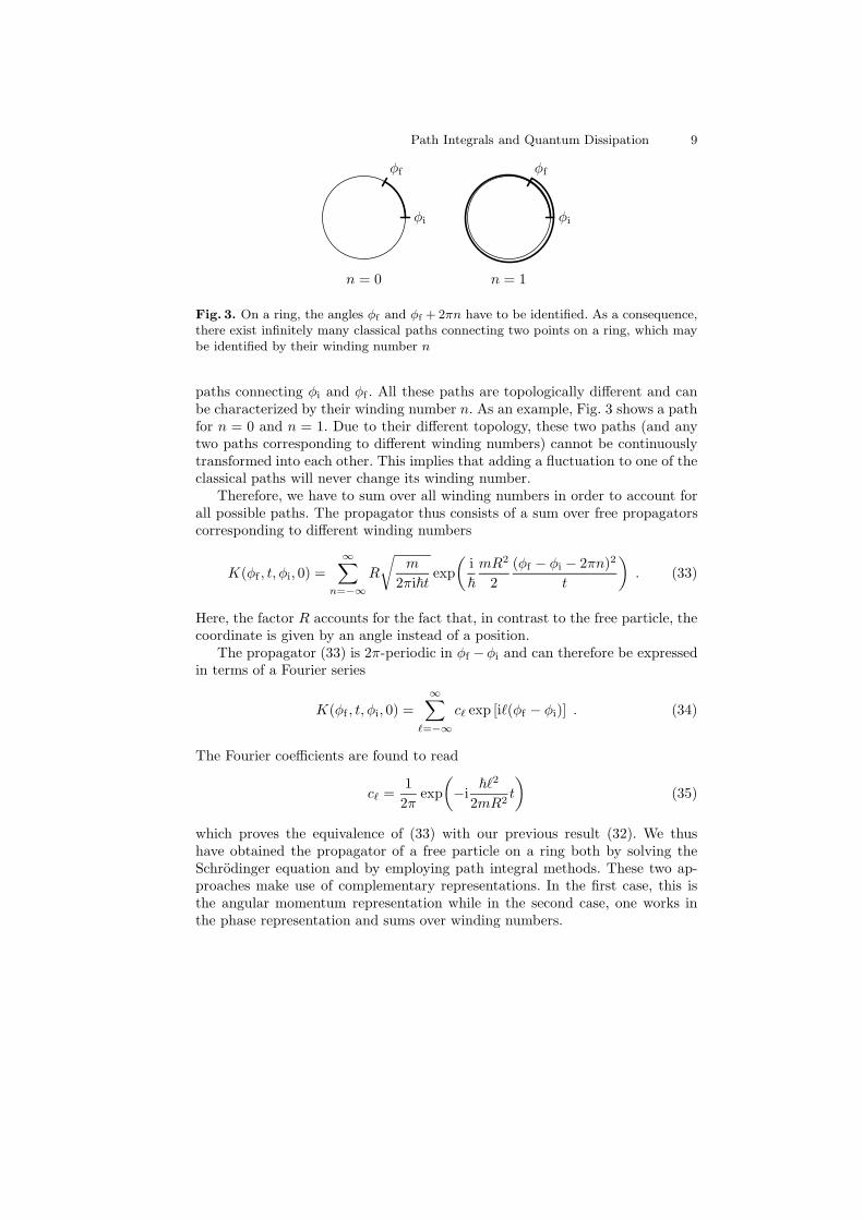
Fig. 3. On a ring, the angles φf and φf + 2πn have to be identified. As a consequence,there exist infinitely many classical paths connecting two points on a ring, which maybe identified by their winding number n
paths connecting φi and φf . All these paths are topologically different and canbe characterized by their winding number n. As an example, Fig. 3 shows a pathfor n = 0 and n = 1. Due to their different topology, these two paths (and anytwo paths corresponding to different winding numbers) cannot be continuouslytransformed into each other. This implies that adding a fluctuation to one of theclassical paths will never change its winding number.
Therefore, we have to sum over all winding numbers in order to account forall possible paths. The propagator thus consists of a sum over free propagatorscorresponding to different winding numbers
K(φf , t, φi, 0) =
∞∑
n=−∞
R
√
m
2πi~texp
(
i
~
mR2
2
(φf − φi − 2πn)2
t
)
. (33)
Here, the factor R accounts for the fact that, in contrast to the free particle, thecoordinate is given by an angle instead of a position.
The propagator (33) is 2π-periodic in φf −φi and can therefore be expressedin terms of a Fourier series
K(φf , t, φi, 0) =
∞∑
ℓ=−∞
cℓ exp [iℓ(φf − φi)] . (34)
The Fourier coefficients are found to read
cℓ =1
2πexp
(
−i~ℓ2
2mR2t
)
(35)
which proves the equivalence of (33) with our previous result (32). We thushave obtained the propagator of a free particle on a ring both by solving theSchrodinger equation and by employing path integral methods. These two ap-proaches make use of complementary representations. In the first case, this isthe angular momentum representation while in the second case, one works inthe phase representation and sums over winding numbers.

10 Gert-Ludwig Ingold
0 xi xf L
1
2
3
4
5
Fig. 4. The reflection at the walls of a box leads to an infinite number of possibletrajectories connecting two points in the box
2.6 Particle in a Box
Another textbook example in standard quantum mechanics is the particle in abox of length L confined by infinitely high walls at x = 0 and x = L. From theeigenvalues
Ej =~
2π2j2
2mL2(36)
with j = 1, 2, . . . and the corresponding eigenfunctions
ψj(x) =
√
2
Lsin(
πjx
L
)
(37)
the propagator is immediately obtained as
K(xf , t, xi, 0) =2
L
∞∑
j=1
exp
(
−i~π2j2
2mL2t
)
sin(
πjxf
L
)
sin(
πjxi
L
)
. (38)
It took some time until this problem was solved within the path integralapproach [9,10]. Here, we have to consider all paths connecting the points xi andxf within a period of time t. Due to the reflecting walls, there again exist infinitelymany classical paths, five of which are depicted in Fig. 4. However, in contrast tothe case of a particle on a ring, these paths are no longer topologically distinct.As a consequence, we may deform a classical path continuously to obtain one ofthe other classical paths.
If, for the moment, we disregard the details of the reflections at the wall, themotion of the particle in a box is equivalent to the motion of a free particle. Thefact that paths are folded back on themselves can be accounted for by takinginto account replicas of the box as shown in Fig. 5. Now, the path does not
necessarily end at x(0)f = xf but at one of the mirror images x
(n)f where n is an
arbitrary integer. In order to obtain the propagator, we will have to sum overall replicas. Due to the different geometry we need to distinguish between thosepaths arising from an even and an odd number of reflections. From Fig. 5 one
Path Integrals and Quantum Dissipation 11
12
34
5
x(−2)f x
(−1)f xf x
(1)f x
(2)fxi
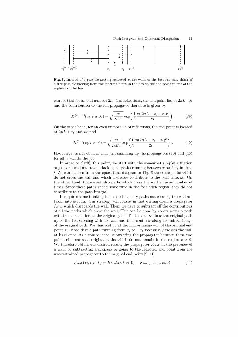
Fig. 5. Instead of a particle getting reflected at the walls of the box one may think ofa free particle moving from the starting point in the box to the end point in one of thereplicas of the box
can see that for an odd number 2n−1 of reflections, the end point lies at 2nL−xf
and the contribution to the full propagator therefore is given by
K(2n−1)(xf , t, xi, 0) =
√
m
2πi~texp
(
i
~
m(2nL− xf − xi)2
2t
)
. (39)
On the other hand, for an even number 2n of reflections, the end point is locatedat 2nL+ xf and we find
K(2n)(xf , t, xi, 0) =
√
m
2πi~texp
(
i
~
m(2nL+ xf − xi)2
2t
)
. (40)
However, it is not obvious that just summing up the propagators (39) and (40)for all n will do the job.
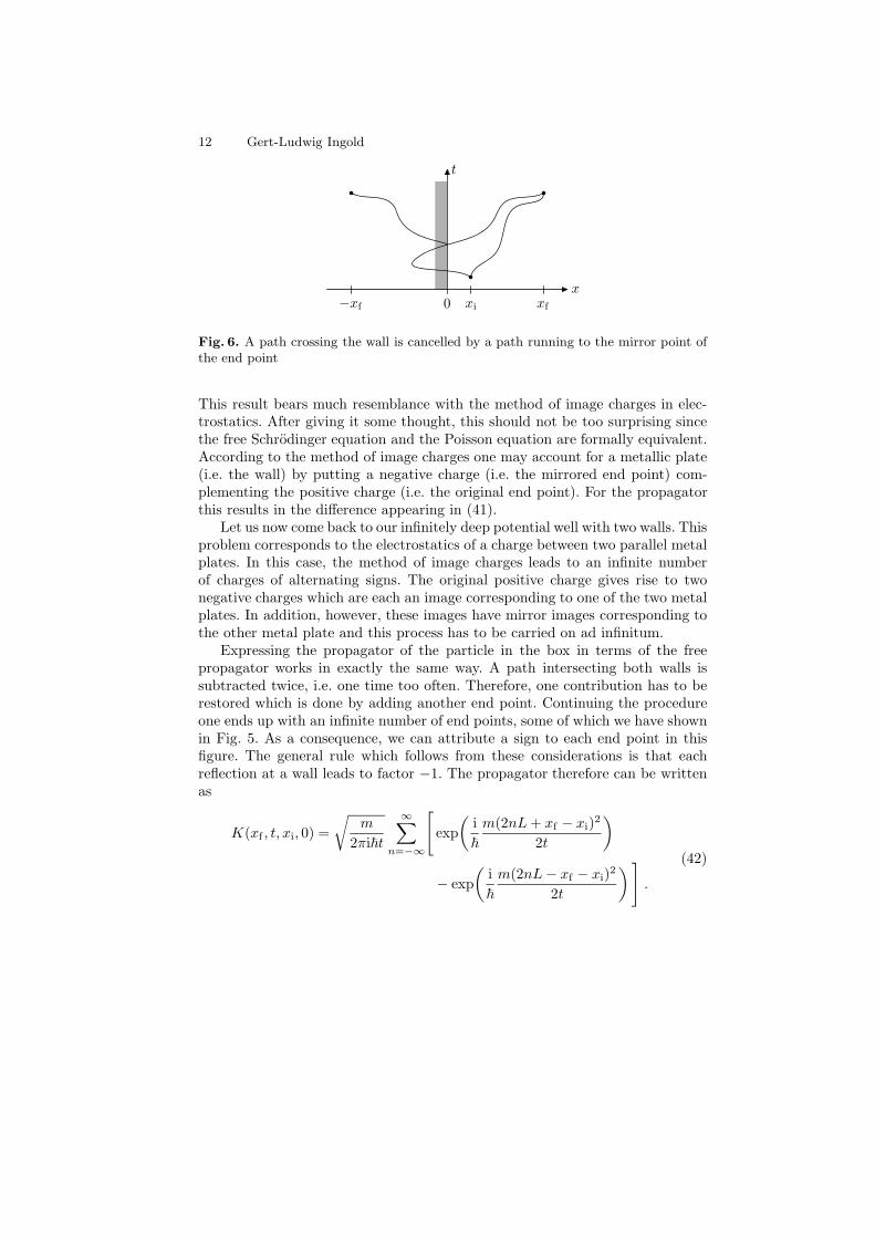
In order to clarify this point, we start with the somewhat simpler situationof just one wall and take a look at all paths running between xi and xf in timet. As can be seen from the space-time diagram in Fig. 6 there are paths whichdo not cross the wall and which therefore contribute to the path integral. Onthe other hand, there exist also paths which cross the wall an even number oftimes. Since these paths spend some time in the forbidden region, they do notcontribute to the path integral.
It requires some thinking to ensure that only paths not crossing the wall aretaken into account. Our strategy will consist in first writing down a propagatorKfree which disregards the wall. Then, we have to subtract off the contributionsof all the paths which cross the wall. This can be done by constructing a pathwith the same action as the original path. To this end we take the original pathup to the last crossing with the wall and then continue along the mirror imageof the original path. We thus end up at the mirror image −xf of the original endpoint xf . Note that a path running from xi to −xf necessarily crosses the wallat least once. As a consequence, subtracting the propagator between these twopoints eliminates all original paths which do not remain in the region x > 0.We therefore obtain our desired result, the propagator Kwall in the presence ofa wall, by subtracting a propagator going to the reflected end point from theunconstrained propagator to the original end point [9–11]
Kwall(xf , t, xi, 0) = Kfree(xf , t, xi, 0) −Kfree(−xf , t, xi, 0) . (41)
12 Gert-Ludwig Ingold
t
xxi xf0−xf
Fig. 6. A path crossing the wall is cancelled by a path running to the mirror point ofthe end point
This result bears much resemblance with the method of image charges in elec-trostatics. After giving it some thought, this should not be too surprising sincethe free Schrodinger equation and the Poisson equation are formally equivalent.According to the method of image charges one may account for a metallic plate(i.e. the wall) by putting a negative charge (i.e. the mirrored end point) com-plementing the positive charge (i.e. the original end point). For the propagatorthis results in the difference appearing in (41).
Let us now come back to our infinitely deep potential well with two walls. Thisproblem corresponds to the electrostatics of a charge between two parallel metalplates. In this case, the method of image charges leads to an infinite numberof charges of alternating signs. The original positive charge gives rise to twonegative charges which are each an image corresponding to one of the two metalplates. In addition, however, these images have mirror images corresponding tothe other metal plate and this process has to be carried on ad infinitum.
Expressing the propagator of the particle in the box in terms of the freepropagator works in exactly the same way. A path intersecting both walls issubtracted twice, i.e. one time too often. Therefore, one contribution has to berestored which is done by adding another end point. Continuing the procedureone ends up with an infinite number of end points, some of which we have shownin Fig. 5. As a consequence, we can attribute a sign to each end point in thisfigure. The general rule which follows from these considerations is that eachreflection at a wall leads to factor −1. The propagator therefore can be writtenas
K(xf , t, xi, 0) =
√
m
2πi~t
∞∑
n=−∞
[
exp
(
i
~
m(2nL+ xf − xi)2
2t
)
− exp
(
i
~
m(2nL− xf − xi)2
2t
)
]
.
(42)

Path Integrals and Quantum Dissipation 13
The symmetries
K(xf + 2L, t, xi, 0) = K(xf , t, xi, 0) (43)
K(−xf , t, xi, 0) = −K(xf , t, xi, 0) (44)
suggest to expand the propagator into the Fourier series
K(xf , t, xi, 0) =
∞∑
j=1
aj(xi, t) sin(
πjxf
L
)
. (45)
Its Fourier coefficients are obtained from (42) as
aj(xi, t) =1
L
∫ L
−L
dxf sin(
πjxf
L
)
K(xf , t, xi, 0)
=2
Lsin(
πjxi
L
)
exp
(
− i
~Ejt
)(46)
where the energies Ej are the eigenenergies of the box defined in (36). Inserting(46) into (45) we thus recover our previous result (38).
2.7 Driven Harmonic Oscillator
Even though the situations dealt with in the previous two sections have been con-ceptually quite interesting, we could in both cases avoid the explicit calculationof a path integral. In the present section, we will introduce the basic techniquesneeded to evaluate path integrals. As an example, we will consider the drivenharmonic oscillator which is simple enough to allow for an exact solution. Inaddition, the propagator will be of use in the discussion of damped quantumsystems in later sections.
Our starting point is the Lagrangian
L =m
2x2 − m
2ω2x2 + xf(t) (47)
of a harmonic oscillator with mass m and frequency ω. The force f(t) may bedue to an external field, e.g. an electric field coupling via dipole interaction to acharged particle. In the context of dissipative quantum mechanics, the harmonicoscillator could represent a degree of freedom of the environment under theinfluence of a force exerted by the system.
According to (28) we obtain the propagator K(xf , t, xi, 0) by calculating theaction for all possible paths starting at time zero at xi and ending at time t atxf . It is convenient to decompose the paths
x(s) = xcl(s) + ξ(s) (48)
into the classical path xcl satisfying the boundary conditions xcl(0) = xi, xcl(t) =xf and a fluctuating part ξ vanishing at the boundaries, i.e. ξ(0) = ξ(t) = 0. Theclassical path has to satisfy the equation of motion
mxcl +mω2xcl = f(s) (49)

14 Gert-Ludwig Ingold
obtained from the Lagrangian (47).For an exactly solvable problem like the driven harmonic oscillator, we could
replace xcl by any path satisfying x(0) = xi, x(t) = xf . We leave it as anexercise to the reader to perform the following calculation with xcl(s) of thedriven harmonic oscillator replaced by xi +(xf −xi)s/t. However, it is importantto note that within the semiclassical approximation discussed in Sect. 2.8 anexpansion around the classical path is essential since this path leads to thedominant contribution to the path integral.
With (48) we obtain for the action
S =
∫ t
0
ds(m
2x2 − m
2ω2x2 + xf(s)
)
=
∫ t
0
ds(m
2x2
cl −m
2ω2x2
cl + xclf(s))
+
∫ t
0
ds(
mxclξ −mω2xclξ + ξf(s))
+
∫ t
0
ds(m
2ξ2 − m
2ω2ξ2
)
. (50)
For our case of a harmonic potential, the third term is independent of the bound-ary values xi and xf as well as of the external driving. The second term vanishesas a consequence of the expansion around the classical path. This can be seenby partial integration and by making use of the fact that xcl is a solution of theclassical equation of motion:
∫ t
0
ds(
mxclξ−mω2xclξ+ ξf(s))
= −∫ t
0
ds(
mxcl +mω2xcl−f(s))
ξ = 0 . (51)
We now proceed in two steps by first determining the contribution of theclassical path and then addressing the fluctuations. The solution of the classicalequation of motion satisfying the boundary conditions reads
xcl(s) = xfsin(ωs)
sin(ωt)+ xi
sin(ω(t− s))
sin(ωt)(52)
+1
mω
[∫ s
0
du sin(ω(s− u))f(u) − sin(ωs)
sin(ωt)
∫ t
0
du sin(ω(t− u))f(u)
]
.
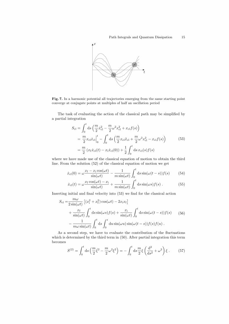
A peculiarity of the harmonic oscillator in the absence of driving is the ap-pearance of conjugate points at times Tn = (π/ω)n where n is an arbitraryinteger. Since the frequency of the oscillations is independent of the amplitude,the position of the oscillator at these times is determined by the initial position:x(T2n+1) = −xi and x(T2n) = xi. This also illustrates the fact mentioned onp. 7, that depending on the boundary conditions there may be more than oneor no classical solution.
Path Integrals and Quantum Dissipation 15
t
x
Fig. 7. In a harmonic potential all trajectories emerging from the same starting pointconverge at conjugate points at multiples of half an oscillation period
The task of evaluating the action of the classical path may be simplified bya partial integration
Scl =
∫ t
0
ds(m
2x2
cl −m
2ω2x2
cl + xclf(s))
=m
2xclxcl
∣
∣
∣
t
0−∫ t
0
ds(m
2xclxcl +
m
2ω2x2
cl − xclf(s))
=m
2(xf xcl(t) − xixcl(0)) +
1
2
∫ t
0
ds xcl(s)f(s)
(53)
where we have made use of the classical equation of motion to obtain the thirdline. From the solution (52) of the classical equation of motion we get
xcl(0) = ωxf − xi cos(ωt)
sin(ωt)− 1
m sin(ωt)
∫ t
0
ds sin(ω(t− s))f(s) (54)
xcl(t) = ωxf cos(ωt) − xi
sin(ωt)+
1
m sin(ωt)
∫ t
0
ds sin(ωs)f(s) . (55)
Inserting initial and final velocity into (53) we find for the classical action
Scl =mω
2 sin(ωt)
[
(x2i + x2
f ) cos(ωt) − 2xixf
]
+xf
sin(ωt)
∫ t
0
ds sin(ωs)f(s) +xi
sin(ωt)
∫ t
0
ds sin(ω(t− s))f(s)
− 1
mω sin(ωt)
∫ t
0
ds
∫ s
0
du sin(ωu) sin(ω(t− s))f(s)f(u) .
(56)
As a second step, we have to evaluate the contribution of the fluctuationswhich is determined by the third term in (50). After partial integration this termbecomes
S(2) =
∫ t
0
ds(m
2ξ2 − m
2ω2ξ2
)
= −∫ t
0
dsm
2ξ
(
d2
ds2+ ω2
)
ξ . (57)

16 Gert-Ludwig Ingold
Here, the superscript ‘(2)’ indicates that this term corresponds to the contri-bution of second order in ξ. In view of the right-hand side it is appropriate toexpand the fluctuation
ξ(s) =
∞∑
n=1
anξn(s) (58)
into eigenfunctions of(
d2
ds2+ ω2
)
ξn = λnξn (59)
with ξn(0) = ξn(t) = 0. As eigenfunctions of a selfadjoint operator, the ξn arecomplete and may be chosen orthonormal. Solving (59) yields the eigenfunctions
ξn(s) =
√
2
tsin(
πns
t
)
(60)
and corresponding eigenvalues
λn = −(πn
t
)2
+ ω2 . (61)
We emphasize that (58) is not the usual Fourier series on an interval of lengtht. Such an expansion could be used in the form
ξ(s) =
√
2
t
∞∑
n=1
[
an
(
cos(2πns
t) − 1
)
+ bn sin(2πns
t)]
(62)
which ensures that the fluctuations vanish at the boundaries. We invite thereader to redo the following calculation with the expansion (62) replacing (58).While at the end the same propagator should be found, it will become clear whythe expansion in terms of eigenfunctions satisfying (59) is preferable.
The integration over the fluctuations now becomes an integration over theexpansion coefficients an. Inserting the expansion (58) into the action one finds
S(2) = −m2
∞∑
n=1
λna2n =
m
2
∞∑
n=1
(
(πn
t
)2
− ω2
)
a2n . (63)
As this result shows, the classical action is only an extremum of the action butnot necessarily a minimum although this is the case for short time intervalst < π/ω. The existence of conjugate points at times Tn = nπ/ω mentionedabove manifests itself here as vanishing of the eigenvalue λn. Then the action isindependent of an which implies that for a time interval Tn all paths xcl + anξnwith arbitrary coefficient an are solutions of the classical equation of motion.
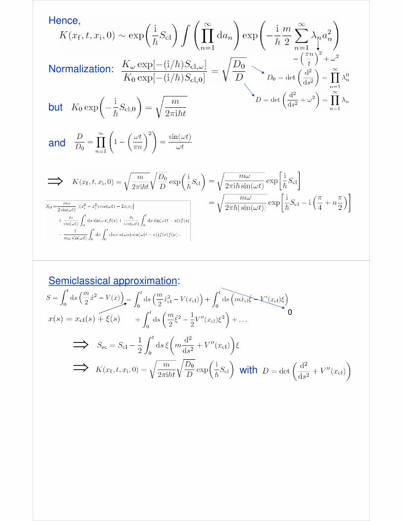
After expansion of the fluctuations in terms of the eigenfunctions (60), thepropagator takes the form
K(xf , t, xi, 0) ∼ exp
(
i
~Scl
)∫
(
∞∏
n=1
dan
)
exp
(
− i
~
m
2
∞∑
n=1
λna2n
)
. (64)
Path Integrals and Quantum Dissipation 17
In principle, we need to know the Jacobi determinant of the transformation fromthe path integral to the integral over the Fourier coefficients. However, since thisJacobi determinant is independent of the oscillator frequency ω, we may alsocompare with the free particle. Evaluating the Gaussian fluctuation integrals,we find for the ratio between the prefactors of the propagators Kω and K0 ofthe harmonic oscillator and the free particle, respectively,
Kω exp[−(i/~)Scl,ω]
K0 exp[−(i/~)Scl,0]=
√
D0
D. (65)
Here, we have introduced the fluctuation determinants for the harmonic oscilla-tor
D = det
(
d2
ds2+ ω2
)
=
∞∏
n=1
λn (66)
and the free particle
D0 = det
(
d2
ds2
)
=
∞∏
n=1
λ0n . (67)
The eigenvalues for the free particle
λ0n = −
(πn
t
)2
(68)
are obtained from the eigenvalues (61) of the harmonic oscillator simply bysetting the frequency ω equal to zero. With the prefactor of the propagator ofthe free particle
K0 exp
(
− i
~Scl,0
)
=
√
m
2πi~t(69)
and (65), the propagator of the harmonic oscillator becomes
K(xf , t, xi, 0) =
√
m
2πi~t
√
D0
Dexp
(
i
~Scl
)
. (70)
For readers unfamiliar with the concept of determinants of differential opera-tors we mention that we may define matrix elements of an operator by projectiononto a basis as is familiar from standard quantum mechanics. The operator rep-resented in its eigenbasis yields a diagonal matrix with the eigenvalues on thediagonal. Then, as for finite dimensional matrices, the determinant is the productof these eigenvalues.
Each of the determinants (66) and (67) by itself diverges. However, we areinterested in the ratio between them which is well-defined [12]
D
D0=
∞∏
n=1
(
1 −(
ωt
πn
)2)
=sin(ωt)
ωt. (71)
18 Gert-Ludwig Ingold
Inserting this result into (70) leads to the propagator of the driven harmonicoscillator in its final form
K(xf , t, xi, 0) =
√
mω
2πi~ sin(ωt)exp
[
i
~Scl
]
=
√
mω
2π~| sin(ωt)| exp
[
i
~Scl − i
(π
4+ n
π
2
)
] (72)
with the classical action defined in (56). The Morse index n in the phase factor isgiven by the integer part of ωt/π. This phase accounts for the changes in sign ofthe sine function [13]. Here, one might argue that it is not obvious which sign ofthe square root one has to take. However, the semigroup property (9) allows toconstruct propagators across conjugate points by joining propagators for shortertime intervals. In this way, the sign may be determined unambiguously [14].
It is interesting to note that the phase factor exp(−inπ/2) in (72) implies thatK(xf , 2π/ω, xi, 0) = −K(xf , 0, xi, 0) = −δ(xf − xi), i.e. the wave function afterone period of oscillation differs from the original wave function by a factor −1.The oscillator thus returns to its original state only after two periods very muchlike a spin-1/2 particle which picks up a sign under rotation by 2π and returnsto its original state only after a 4π-rotation. This effect might be observed inthe case of the harmonic oscillator by letting interfere the wave functions of twooscillators with different frequency [15].
2.8 Semiclassical Approximation
The systems considered so far have been special in the sense that an exactexpression for the propagator could be obtained. This is a consequence of thefact that the potential was at most quadratic in the coordinate. Unfortunately,in most cases of interest the potential is more complicated and apart from a fewexceptions an exact evaluation of the path integral turns out to be impossible.To cope with such situations, approximation schemes have been devised. In thefollowing, we will restrict ourselves to the most important approximation whichis valid whenever the quantum fluctuations are small or, equivalently, when theactions involved are large compared to Planck’s constant so that the latter maybe considered to be small.
The decomposition of a general path into the classical path and fluctuationsaround it as employed in (48) in the previous section was merely a matter ofconvenience. For the exactly solvable case of a driven harmonic oscillator itis not really relevant how we express a general path satisfying the boundaryconditions. Within the semiclassical approximation, however, it is decisive toexpand around the path leading to the dominant contribution, i.e. the classicalpath. From a more mathematical point of view, we have to evaluate a pathintegral over exp(iS/~) for small ~. This can be done in a systematic way by themethod of stationary phase where the exponent has to be expanded around theextrema of the action S.
Path Integrals and Quantum Dissipation 19
x/√α
Re[
exp(iαx2)]
−1 1
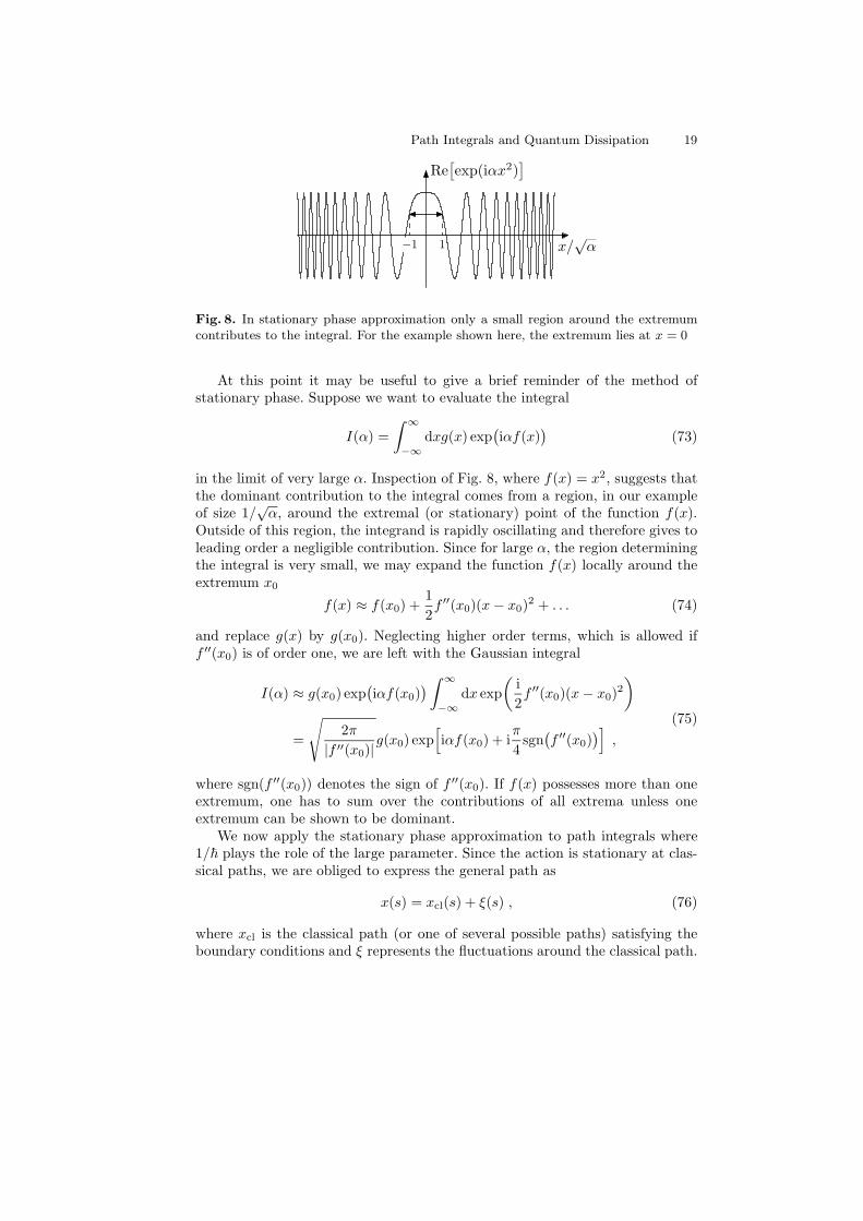
Fig. 8. In stationary phase approximation only a small region around the extremumcontributes to the integral. For the example shown here, the extremum lies at x = 0
At this point it may be useful to give a brief reminder of the method ofstationary phase. Suppose we want to evaluate the integral
I(α) =
∫ ∞
−∞
dxg(x) exp(
iαf(x))
(73)
in the limit of very large α. Inspection of Fig. 8, where f(x) = x2, suggests thatthe dominant contribution to the integral comes from a region, in our exampleof size 1/
√α, around the extremal (or stationary) point of the function f(x).
Outside of this region, the integrand is rapidly oscillating and therefore gives toleading order a negligible contribution. Since for large α, the region determiningthe integral is very small, we may expand the function f(x) locally around theextremum x0
f(x) ≈ f(x0) +1
2f ′′(x0)(x − x0)
2 + . . . (74)
and replace g(x) by g(x0). Neglecting higher order terms, which is allowed iff ′′(x0) is of order one, we are left with the Gaussian integral
I(α) ≈ g(x0) exp(
iαf(x0))
∫ ∞
−∞
dx exp
(
i
2f ′′(x0)(x − x0)
2
)
=
√
2π
|f ′′(x0)|g(x0) exp
[
iαf(x0) + iπ
4sgn(
f ′′(x0))
]
,
(75)
where sgn(f ′′(x0)) denotes the sign of f ′′(x0). If f(x) possesses more than oneextremum, one has to sum over the contributions of all extrema unless oneextremum can be shown to be dominant.
We now apply the stationary phase approximation to path integrals where1/~ plays the role of the large parameter. Since the action is stationary at clas-sical paths, we are obliged to express the general path as
x(s) = xcl(s) + ξ(s) , (76)
where xcl is the classical path (or one of several possible paths) satisfying theboundary conditions and ξ represents the fluctuations around the classical path.
20 Gert-Ludwig Ingold
With this decomposition the action becomes
S =
∫ t
0
ds(m
2x2 − V (x)
)
=
∫ t
0
ds(m
2x2
cl − V (xcl))
+
∫ t
0
ds(
mxclξ − V ′(xcl)ξ)
+
∫ t
0
ds
(
m
2ξ2 − 1
2V ′′(xcl)ξ
2
)
+ . . .
(77)
It is instructive to compare this result with the action (50) for the driven har-monic oscillator. Again, the first term represents the classical action. The secondterm vanishes as was shown explicitly in (51) for the driven oscillator. In thegeneral case, one can convince oneself by partial integration of the kinetic partand comparison with the classical equation of motion that this term vanishesagain. This is of course a consequence of the fact that the classical path, aroundwhich we expand, corresponds to an extremum of the action. The third term onthe right-hand-side of (77) is the leading order term in the fluctuations as wasthe case in (50). There is however an important difference since for anharmonicpotentials the second derivative of the potential V ′′ is not constant and there-fore the contribution of the fluctuations depends on the classical path. Finally,in general there will be higher order terms in the fluctuations as indicated by thedots in (77). The semiclassical approximation consists in neglecting these higherorder terms so that after a partial integration, we get for the action
Ssc = Scl −1
2
∫ t
0
ds ξ
(
md2
ds2+ V ′′(xcl)
)
ξ (78)
where the index ‘sc’ indicates the semiclassical approximation.Before deriving the propagator in semiclassical approximation, we have to
discuss the regime of validity of this approximation. Since the first term in (78)gives only rise to a global phase factor, it is the second term which determines themagnitude of the quantum fluctuations. For this term to contribute, we shouldhave ξ2/~ . 1 so that the magnitude of typical fluctuations is at most of order√
~. The term of third order in the fluctuations is already smaller than the secondorder term by a factor (
√~)3/~ =
√~. If Planck’s constant can be considered
to be small, we may indeed neglect the fluctuation contributions of higher thansecond order except for one exception: It may happen that the second order termdoes not contribute, as has been the case at the conjugate points for the drivenharmonic oscillator in Sect. 2.7. Then, the leading nonvanishing contributionbecomes dominant. For the following discussion, we will not consider this lattercase.
In analogy to Sect. 2.7 we obtain for the propagator in semiclassical approx-imation
K(xf , t, xi, 0) =
√
m
2πi~t
√
D0
Dexp
(
i
~Scl
)
(79)
Path Integrals and Quantum Dissipation 21
where
D = det
(
d2
ds2+ V ′′(xcl)
)
(80)
and D0 is the fluctuation determinant (67) of the free particle.Even though it may seem that determining the prefactor is a formidable task
since the fluctuation determinant for a given potential has to be evaluated, thistask can be greatly simplified. In addition, the following considerations offer thebenefit of providing a physical interpretation of the prefactor. In our evaluationof the prefactor we follow Marinov [16]. The main idea is to make use of thesemigroup property (9) of the propagator
C(xf , t, xi, 0) exp
[
i
~Scl(xf , t, xi, 0)
]
(81)
=
∫
dx′C(xf , t, x′, t′)C(x′, t′, xi, 0) exp
[
i
~
[
Scl(xf , t, x′, t′) + Scl(x
′, t′, xi, 0)]
]
where the prefactor C depends on the fluctuation contribution. We now haveto evaluate the x′-integral within the semiclassical approximation. According tothe stationary phase requirement discussed above, the dominant contribution tothe integral comes from x′ = x0(xf , xi, t, t
′) satisfying
∂Scl(xf , t, x′, t′)
∂x′
∣
∣
∣
∣
x′=x0
+∂Scl(x
′, t′, xi, 0)
∂x′
∣
∣
∣
∣
x′=x0
= 0 . (82)
According to classical mechanics these derivatives are related to initial and finalmomentum by [17]
(
∂Scl
∂xi
)
xf ,tf ,ti
= −pi
(
∂Scl
∂xf
)
xi,tf ,ti
= pf (83)
so that (82) can expressed as
p(t′ − ε) = p(t′ + ε) . (84)
The point x0 thus has to be chosen such that the two partial classical pathscan be joined with a continuous momentum. Together they therefore yield thecomplete classical path and in particular
Scl(xf , t, xi, 0) = Scl(xf , t, x0, t′) + Scl(x0, t
′, xi, 0) . (85)
This relation ensures that the phase factors depending on the classical actionson both sides of (81) are equal.
After having identified the stationary path, we have to evaluate the integralover x′ in (81). Within semiclassical approximation this Gaussian integral leadsto
C(xf , t, xi, 0)
C(xf , t, x0, t′)C(x0, t′, xi, 0)(86)
=
(
1
2πi~
∂2
∂x20
[
Scl(xf , t, x0, t′) + Scl(x0, t
′, xi, 0)]
)−1/2
.
22 Gert-Ludwig Ingold
In order to make progress, it is useful to take the derivative of (85) with respectto xf and xi. Keeping in mind that x0 depends on these two variables one finds
∂2Scl(xf , t, xi, 0)
∂xf∂xi=∂2Scl(xf , t, x0, t
′)
∂xf∂x0
∂x0
∂xi+∂2Scl(x0, t
′, xi, 0)
∂xi∂x0
∂x0
∂xf
+∂2
∂x20
[
Scl(xf , t, x0, t′) + Scl(x0, t
′, xi, t)]∂x0
∂xi
∂x0
∂xf.
(87)
Similarly, one finds by taking derivatives of the stationary phase condition (82)
∂x0
∂xf= −
∂2
∂xfx0Scl(xf , t, x0, t
′)
∂2
∂x20
[
Scl(xf , t, x0, t′) + Scl(x0, t′, xi, 0)]
(88)
and
∂x0
∂xi= −
∂2
∂xix0Scl(x0, t
′, xi, 0)
∂2
∂x20
[
Scl(xf , t, x0, t′) + Scl(x0, t′, xi, 0)]
. (89)
These expressions allow to eliminate the partial derivatives of x0 with respectto xi and xf appearing in (87) and one finally obtains
(
∂2
∂x20
[
Scl(xf , t, x0, t′) + Scl(x0, t
′, xi, 0)]
)−1
(90)
= −
∂2
∂xi∂xfScl(xf , t, xi, 0)
∂2Scl(xf , t, x0, t′)
∂xf∂x0
∂2Scl(x0, t′, xi, 0)
∂xi∂x0
.
Inserting this result into (86), the prefactor can be identified as the so-calledVan Vleck-Pauli-Morette determinant [18–20]
C(xf , t, xi, 0) =
[
1
2πi~
(
−∂2Scl(xf , t, xi, 0)
∂xf∂xi
)]1/2
(91)
so that the propagator in semiclassical approximation finally reads
K(xf , t, xi, 0) (92)
=
(
1
2π~
∣
∣
∣
∣
−∂2Scl(xf , t, xi, 0)
∂xf∂xi
∣
∣
∣
∣
)1/2
exp
[
i
~Scl(xf , t, xi, 0) − i
(π
4+ n
π
2
)
]
where the Morse index n denotes the number of sign changes of ∂2Scl/∂xf∂xi
[13]. We had encountered such a phase factor before in the propagator (72) ofthe harmonic oscillator.
Path Integrals and Quantum Dissipation 23
As we have already mentioned above, derivatives of the action with respectto position are related to momenta. This allows to give a physical interpretationof the prefactor of the propagator as the change of the end point of the path asa function of the initial momentum
(
− ∂2Scl
∂xi∂xf
)−1
=∂xf
∂pi. (93)
A zero of this expression, or equivalently a divergence of the prefactor of thepropagator, indicates a conjugate point where the end point does not depend onthe initial momentum.
To close this section, we want to compare the semiclassical result (92) withexact results for the free particle and the harmonic oscillator. In our discussionof the free particle in Sect. 2.3 we already mentioned that the propagator canbe expressed entirely in terms of classical quantities. Indeed, the expression (19)for the propagator of the free particle agrees with (92).
For the harmonic oscillator, we know from Sect. 2.7 that the prefactor doesnot depend on a possibly present external force. We may therefore consider theaction (56) in the absence of driving f(s) = 0 which then reads
Scl =mω
2 sin(ωt)
[(
x2i + x2
f
)
cos(ωt) − 2xixf
]
. (94)
Taking the derivative with respect to xi and xf one finds for the prefactor
C(xf , t, xi, 0) =
(
mω
2πi~ sin(ωt)
)1/2
(95)
which is identical with the prefactor in our previous result (72). As expected,for potentials at most quadratic in the coordinate the semiclassical propagatoragrees with the exact expression.
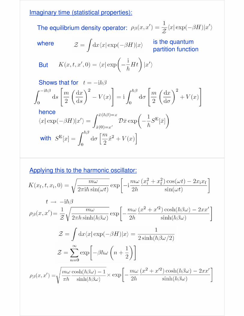
2.9 Imaginary Time Path Integral
In the discussion of dissipative systems we will be dealing with a system cou-pled to a large number of environmental degrees of freedom. In most cases, theenvironment will act like a large heat bath characterized by a temperature T .The state of the environment will therefore be given by an equilibrium densitymatrix. Occasionally, we may also be interested in the equilibrium density ma-trix of the system itself. Such a state may be reached after equilibration due toweak coupling with a heat bath.
In order to describe such thermal equilibrium states and the dynamics ofthe system on a unique footing, it is desirable to express equilibrium densitymatrices in terms of path integrals. This is indeed possible as one recognizes bywriting the equilibrium density operator in position representation
ρβ(x, x′) =1
Z 〈x| exp(−βH)|x′〉 (96)
24 Gert-Ludwig Ingold
with the partition function
Z =
∫
dx〈x| exp(−βH)|x〉 . (97)
Comparing with the propagator in position representation
K(x, t, x′, 0) = 〈x| exp
(
− i
~Ht
)
|x′〉 (98)
one concludes that apart from the partition function the equilibrium densitymatrix is equivalent to a propagator in imaginary time t = −i~β.
After the substitution σ = is the action in imaginary time −i~β reads
∫ −i~β
0
ds
[
m
2
(
dx
ds
)2
− V (x)
]
= i
∫
~β
0
dσ
[
m
2
(
dx
dσ
)2
+ V (x)
]
. (99)
Here and in the following, we use greek letters to indicate imaginary times.Motivated by the right-hand side of (99) we define the so-called Euclidean action
SE[x] =
∫ ~β
0
dσ[m
2x2 + V (x)
]
. (100)
Even though one might fear a lack of intuition for motion in imaginary time, thisresults shows that it can simply be thought of as motion in the inverted potentialin real time. With the Euclidean action (100) we now obtain as an importantresult the path integral expression for the (unnormalized) equilibrium densitymatrix
〈x| exp(−βH)|x′〉 =
∫ x(~β)=x
x(0)=x′
Dx exp
(
−1
~SE[x]
)
. (101)
This kind of functional integral was discussed as early as 1923 by Wiener [21] inthe context of classical Brownian motion.
As an example we consider the (undriven) harmonic oscillator. There is ac-tually no need to evaluate a path integral since we know already from Sect. 2.7the propagator
K(xf , t, xi, 0) =
√
mω
2πi~ sin(ωt)exp
[
−imω
2~
(x2i + x2
f ) cos(ωt) − 2xixf
sin(ωt)
]
. (102)
Transforming the propagator into imaginary time t → −i~β and renaming xi
and xf into x′ and x, respectively, one obtains the equilibrium density matrix
ρβ(x, x′) (103)
=1
Z
√
mω
2π~ sinh(~βω)exp
[
−mω2~
(x2 + x′2) cosh(~βω) − 2xx′
sinh(~βω)
]
.
The partition function is obtained by performing the trace as
Z =
∫
dx〈x| exp(−βH)|x〉 =1
2 sinh(~βω/2)(104)
Path Integrals and Quantum Dissipation 25
which agrees with the expression
Z =∞∑
n=0
exp
[
−β~ω
(
n+1
2
)]
(105)
based on the energy levels of the harmonic oscillator.Since the partition function often serves as a starting point for the calculation
of thermodynamic properties, it is instructive to take a closer at how this quan-tity may be obtained within the path integral formalism. A possible approachis the one we just have sketched. By means of an imaginary time path integralone first calculates 〈x| exp(−βH)|x〉 which is proportional to the probability tofind the system at position x. Subsequent integration over coordinate space thenyields the partition function.
However, the partition function may also be determined in one step. To thisend, we expand around the periodic trajectory with extremal Euclidean actionwhich in our case is given by x(σ) = 0. Any deviation will increase both thekinetic and potential energy and thus increase the Euclidean action. All othertrajectories contributing to the partition function are generated by a Fourierseries on the imaginary time interval from 0 to ~β
x(σ) =1√~β
[
a0 +√
2
∞∑
n=1
(
an cos(νnσ) + bn sin(νnσ))
]
(106)
where we have introduced the so-called Matsubara frequencies
νn =2π
~βn . (107)
This ansatz should be compared with (62) for the fluctuations where a0 wasfixed because the fluctuations had to vanish at the boundaries. For the partitionfunction this requirement is dropped since we have to integrate over all periodictrajectories. Furthermore, we note that indeed with the ansatz (106) only theperiodic trajectories contribute. All other paths cost an infinite amount of actiondue to the jump at the boundary as we will see shortly.
Inserting the Fourier expansion (106) into the Euclidean action of the har-monic oscillator
SE =
∫
~β
0
dσm
2
(
x2 + ω2x2)
(108)
we find
SE =m
2
[
ω2a20 +
∞∑
n=1
(ν2n + ω2)(a2
n + b2n)
]
. (109)
As in Sect. 2.7 we do not want to go into the mathematical details of integrationmeasures and Jacobi determinants. Unfortunately, the free particle cannot serveas a reference here because its partition function does not exist. We thereforecontent ourselves with remarking that because of
1
ω
∞∏
n=1
1
ν2n + ω2
=~β
∑∞
n=1 ν2n
1
2 sinh(~βω/2)(110)
26 Gert-Ludwig Ingold
the result of the Gaussian integral over the Fourier coefficients yields the parti-tion function up to a frequency independent factor. This enables us to determinethe partition function in more complicated cases by proceeding as above and us-ing the partition function harmonic oscillator as a reference.
Returning to the density matrix of the harmonic oscillator we finally obtainby inserting the partition function (104) into the expression (103) for the densitymatrix
ρβ(x, x′) =
√
mω
π~
cosh(~βω) − 1
sinh(~βω)(111)
× exp
[
−mω2~
(x2 + x′2) cosh(~βω) − 2xx′
sinh(~βω)
]
.
Without path integrals, this result would require the evaluation of sums overHermite polynomials.
The expression for the density matrix (111) can be verified in the limits ofhigh and zero temperature. In the classical limit of very high temperatures, theprobability distribution in real space is given by
P (x) = ρβ(x, x) =
√
βmω2
2πexp
(
−βmω2
2x2
)
∼ exp[−βV (x)] . (112)
We thus have obtained the Boltzmann distribution which depends only on thepotential energy. The fact that the kinetic energy does not play a role can easilybe understood in terms of the path integral formalism. Excursions in a very shorttime ~β cost too much action and are therefore strongly suppressed.
In the opposite limit of zero temperature the density matrix factorizes intoa product of ground state wave functions of the harmonic oscillator
limβ→∞
ρβ(x, x′) =
[
(mω
π~
)1/4
exp(
−mω2~
x2)
][
(mω
π~
)1/4
exp(
−mω2~
x′2)
]
(113)
as should be expected.
3 Dissipative Systems
3.1 Introduction
In classical mechanics dissipation can often be adequately described by includinga velocity dependent damping term into the equation of motion. Such a phe-nomenological approach is no longer possible in quantum mechanics where theHamilton formalism implies energy conservation for time-independent Hamilto-nians. Then, a better understanding of the situation is necessary in order toarrive at an appropriate physical model.
A damped pendulum may help us to understand the mechanism of dissipa-tion. The degree of freedom of interest, the elongation of the pendulum, under-goes a damped motion because it interacts with other degrees of freedom, the

Path Integrals and Quantum Dissipation 27
molecules in the air surrounding the pendulum’s mass. We may consider thependulum and the air molecules as one large system which, if assumed to beisolated from further degrees of freedom, obeys energy conservation. The energyof the pendulum alone, however, will in general not be conserved. This singledegree of freedom is therefore subject to dissipation arising from the coupling toother degrees of freedom.
This insight will allow us in the following section to introduce a model for asystem coupled to an environment and to demonstrate explicitly its dissipativenature. In particular, we will introduce the quantities needed for a descriptionwhich focuses on the system degree of freedom. We are then in a position toreturn to the path integral formalism and to demonstrate how it may be em-ployed to study dissipative systems. Starting from the model of system andenvironment, the latter will be eliminated to obtain a reduced description forthe system alone. This leaves us with an effective action which forms the basisof the path integral description of dissipation.
3.2 Environment as Collection of Harmonic Oscillators
A suitable model for dissipative quantum systems should both incorporate theidea of a coupling between system and environment and be amenable to ananalytic treatment of the environmental coupling. These requirements are metby a model which nowadays is often referred to as Caldeira-Leggett model [22,23]even though it has been discussed in the literature under various names beforefor harmonic systems [24–27] and anharmonic systems [28]. The Hamiltonian
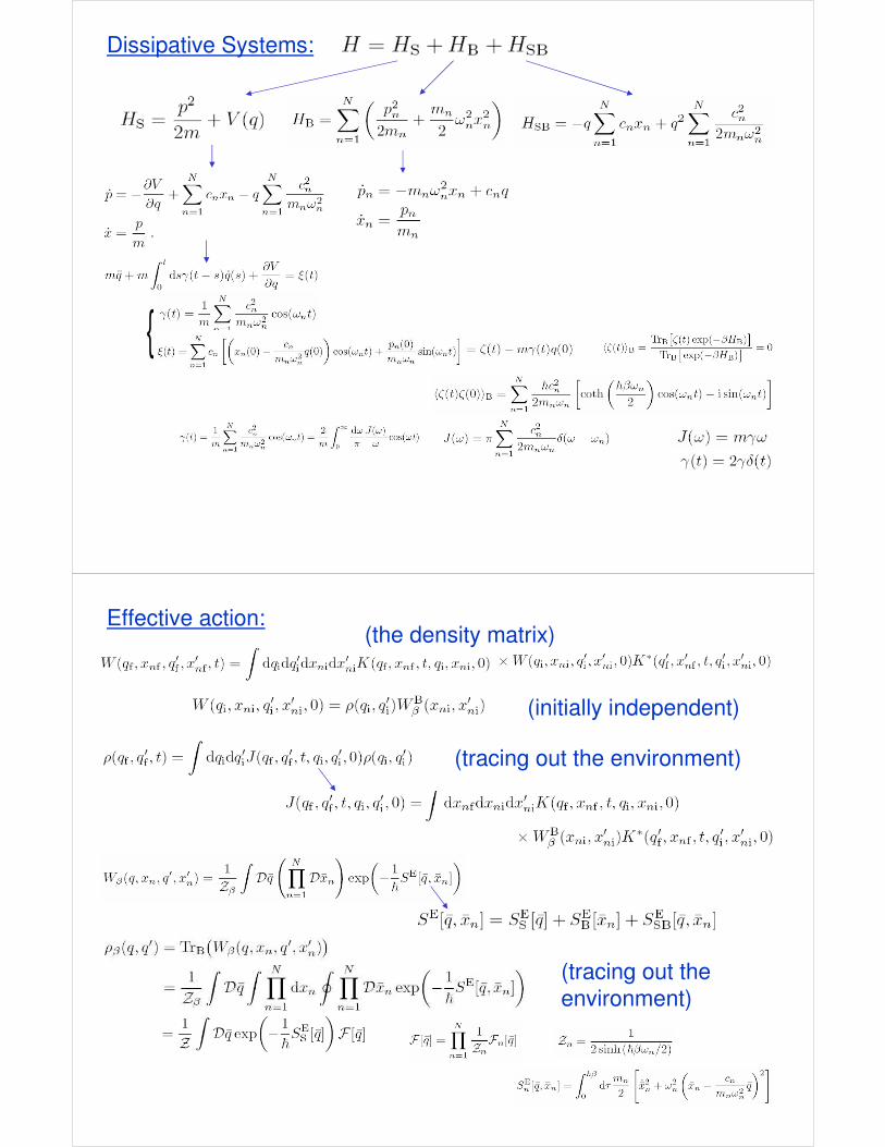
H = HS +HB +HSB (114)
consists of three contributions. The Hamiltonian of the system degree of freedom
HS =p2
2m+ V (q) (115)
models a particle of mass m moving in a potential V . Here, we denote thecoordinate by q to facilitate the distinction from the environmental coordinatesxn which we will introduce in a moment. Of course, the system degree of freedomdoes not have to be associated with a real particle but may be quite abstract. Infact, a substantial part of the calculations to be discussed in the following doesnot depend on the detailed form of the system Hamiltonian.
The Hamiltonian of the environmental degrees of freedom
HB =
N∑
n=1
(
p2n
2mn+mn
2ω2
nx2n
)
(116)
describes a collection of harmonic oscillators. While the properties of the envi-ronment may in some cases be chosen on the basis of a microscopic model, thisdoes not have to be the case. Often, a phenomenological approach is sufficientas we will see below. As an example we mention an Ohmic resistor which as a
28 Gert-Ludwig Ingold
linear electric element should be well described by a Hamiltonian of the form(116). On the other hand, the underlying mechanism leading to dissipation, e.g.in a resistor, may be much more complicated than that implied by the model ofa collection of harmonic oscillators.
The coupling defined by the Hamiltonian
HSB = −qN∑
n=1
cnxn + q2N∑
n=1
c2n2mnω2
n
(117)
is bilinear in the position operators of system and environment. There are caseswhere the bilinear coupling is realistic, e.g. for an environment consisting of alinear electric circuit like the resistor just mentioned or for a dipolar couplingto electromagnetic field modes encountered in quantum optics. Within a moregeneral scope, this Hamiltonian may be viewed as linearization of a nonlinearcoupling in the limit of weak coupling to the environmental degrees of freedom.As was first pointed out by Caldeira and Leggett, an infinite number of degreesof freedom still allows for strong damping even if each environmental oscillatorcouples only weakly to the system [22,23].
An environment consisting of harmonic oscillators as in (116) might be criti-cized. If the potential V (q) is harmonic, one may pass to normal coordinates andthus demonstrate that after some time a revival of the initial state will occur.For sufficiently many environmental oscillators, however, this so-called Poincarerecurrence time tends to infinity [29]. Therefore, even with a linear environmentirreversibility becomes possible at least for all practical purposes.
The reader may have noticed that in the coupling Hamiltonian (117) a termis present which only contains an operator acting in the system Hilbert spacebut depends on the coupling constants cn. The physical reason for the inclusionof this term lies in a potential renormalization introduced by the first term in(117). This becomes clear if we consider the minimum of the Hamiltonian withrespect to the system and environment coordinates. From the requirement
∂H
∂xn= mnω
2nxn − cnq
!= 0 (118)
we obtainxn =
cnmnω2
n
q . (119)
Using this result to determine the minimum of the Hamiltonian with respect tothe system coordinate we find
∂H
∂q=∂V
∂q−
N∑
n=1
cnxn + q
N∑
n=1
c2nmnω2
n
=∂V
∂q. (120)
The second term in (117) thus ensures that this minimum is determined by thebare potential V (q).
After having specified the model, we now want to derive an effective de-scription of the system alone. It was first shown by Magalinskiı [24] that the
Path Integrals and Quantum Dissipation 29
elimination of the environmental degrees of freedom leads indeed to a dampedequation of motion for the system coordinate. We perform the elimination withinthe Heisenberg picture where the evolution of an operator A is determined by
dA
dt=
i
~[H,A] . (121)
From the Hamiltonian (114) we obtain the equations of motion for the environ-mental degrees of freedom
pn = −mnω2nxn + cnq
xn =pn
mn
(122)
and the system degree of freedom
p = −∂V∂q
+
N∑
n=1
cnxn − q
N∑
n=1
c2nmnω2
n
x =p
m.
(123)
The trick for solving the environmental equations of motion (122) consistsin treating the system coordinate q(t) as if it were a given function of time. Theinhomogeneous differential equation then has the solution
xn(t) = xn(0) cos(ωnt) +pn(0)
mnωnsin(ωnt) +
cnmnωn
∫ t
0
ds sin(
ωn(t− s))
q(s) .
(124)Inserting this result into (123) one finds an effective equation of motion for thesystem coordinate
mq −∫ t
0
ds
N∑
n=1
c2nmnωn
sin(
ωn(t− s))
q(s) +∂V
∂q+ q
N∑
n=1
c2nmnω2
n
(125)
=N∑
n=1
cn
[
xn(0) cos(ωnt) +pn(0)
mnωnsin(ωnt)
]
.
By a partial integration of the second term on the left-hand side this equationof motion can be cast into its final form
mq +m
∫ t
0
dsγ(t− s)q(s) +∂V
∂q= ξ(t) (126)
with the damping kernel
γ(t) =1
m
N∑
n=1
c2nmnω2
n
cos(ωnt) (127)

30 Gert-Ludwig Ingold
and the operator-valued fluctuating force
ξ(t) =N∑
n=1
cn
[(
xn(0) − cnmnω2
n
q(0)
)
cos(ωnt) +pn(0)
mnωnsin(ωnt)
]
. (128)
The fluctuating force vanishes if averaged over a thermal density matrix ofthe environment including the coupling to the system
〈ξ(t)〉B+SB =TrB
[
ξ(t) exp(
−β(HB +HSB))]
TrB[
exp(
−β(HB +HSB))] = 0 . (129)
For weak coupling, one may want to split off the transient term mγ(t)q(0) whichis of second order in the coupling and write the fluctuating force as [30]
ξ(t) = ζ(t) −mγ(t)q(0) . (130)
The so defined force ζ(t) vanishes if averaged over the environment alone
〈ζ(t)〉B =TrB
[
ζ(t) exp(−βHB)]
TrB[
exp(−βHB)] = 0 . (131)
An important quantity to characterize the fluctuating force is the correla-tion function which again can be evaluated for ξ with respect to HB +HSB orequivalently for ζ with respect to HB alone. With (128) and (130) we get thecorrelation function
〈ζ(t)ζ(0)〉B =∑
n,l
cncl
⟨(
xn(0) cos(ωnt) +pn(0)
mnωisin(ωnt)
)
xl(0)
⟩
B
. (132)
In thermal equilibrium the second moments are given by
〈xn(0)xl(0)〉B = δnl~
2mnωncoth
(
~βωn
2
)
(133)
〈pn(0)xl(0)〉B = − i~
2δnl , (134)
so that the noise correlation function finally becomes
〈ζ(t)ζ(0)〉B =N∑
n=1
~c2n2mnωn
[
coth
(
~βωn
2
)
cos(ωnt) − i sin(ωnt)
]
. (135)
The imaginary part appearing here is a consequence of the fact that the operatorsζ(t) and ζ(0) in general do not commute. The correlation function (135) appearsas integral kernel both in master equations as well as in the effective actionderived below (cf. (168) and (169)).

Path Integrals and Quantum Dissipation 31
It is remarkable that within a reduced description for the system alone allquantities characterizing the environment may be expressed in terms of the spec-tral density of bath oscillators
J(ω) = π
N∑
n=1
c2n2mnωn
δ(ω − ωn) . (136)
As an example, the damping kernel may be expressed in terms of this spectraldensity as
γ(t) =1
m
N∑
n=1
c2nmnω2
n
cos(ωnt) =2
m
∫ ∞
0
dω
π
J(ω)
ωcos(ωt) . (137)
For practical calculations, it is therefore unnecessary to specify all parametersmn, ωn and cn appearing in (116) and (117). It rather suffices to define thespectral density J(ω).
The most frequently used spectral density
J(ω) = mγω (138)
is associated with the so-called Ohmic damping. This term is sometimes em-ployed to indicate a proportionality to frequency merely at low frequencies in-stead of over the whole frequency range. In fact, in any realistic situation thespectral density will not increase like in (138) for arbitrarily high frequencies.It is justified to use the term “Ohmic damping” even if (138) holds only be-low a certain frequency provided this frequency is much higher than the typicalfrequencies appearing in the system dynamics.
From (137) one finds the damping kernel for Ohmic damping
γ(t) = 2γδ(t) , (139)
which renders (126) memory-free. We thus recover the velocity proportionaldamping term familiar from classical damped systems. It should be noted thatthe factor of two in (139) disappears upon integration in (126) since (137) impliesthat the delta function is symmetric around zero.
At this point, we want to briefly elucidate the origin of the term “Ohmicdamping”. Let us consider the electric circuit shown in Fig. 9 consisting of aresistance R, a capacitance C and an inductance L. Summing up the voltagesaround the loop, one obtains as equation of motion for the charge Q on thecapacitor
LQ+RQ+Q
C= 0 , (140)
which shows that an Ohmic resistor leads indeed to memoryless damping. Theseconsiderations demonstrate that even without knowledge of the microscopic ori-gin of dissipation in a resistor, we may employ the Ohmic spectral density (138)to account for its dissipative nature.
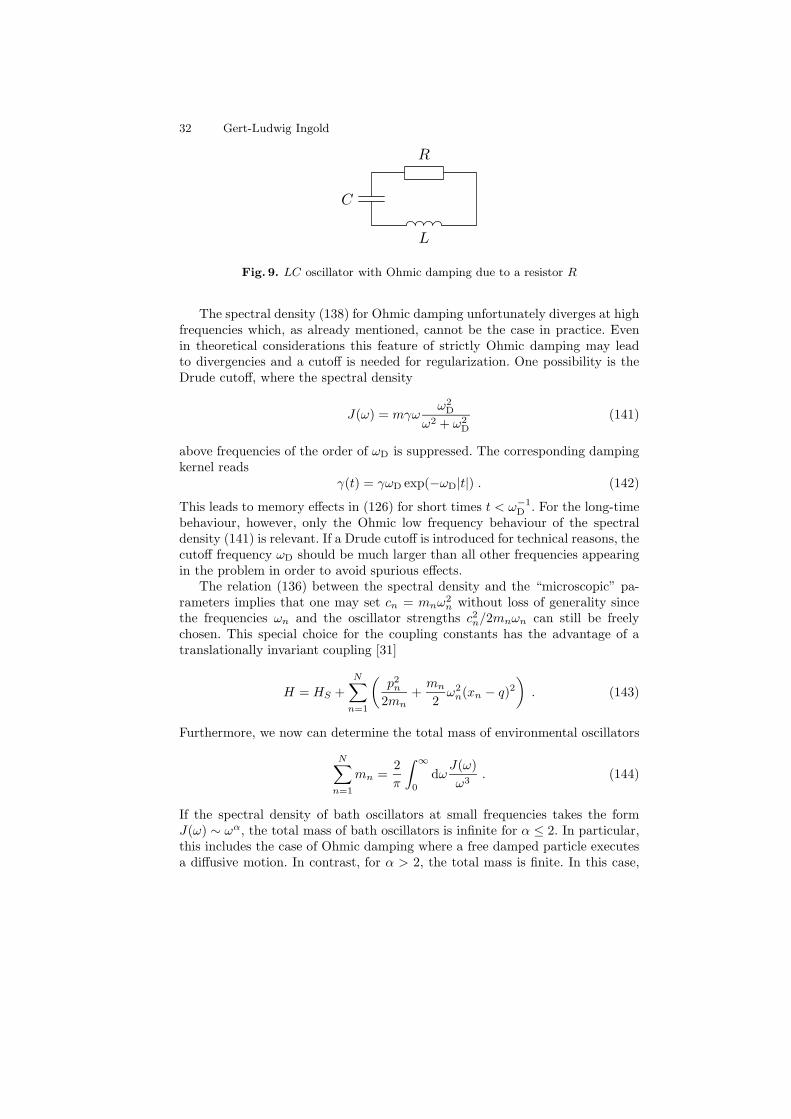
32 Gert-Ludwig Ingold
R
L
C
Fig. 9. LC oscillator with Ohmic damping due to a resistor R
The spectral density (138) for Ohmic damping unfortunately diverges at highfrequencies which, as already mentioned, cannot be the case in practice. Evenin theoretical considerations this feature of strictly Ohmic damping may leadto divergencies and a cutoff is needed for regularization. One possibility is theDrude cutoff, where the spectral density
J(ω) = mγωω2
D
ω2 + ω2D
(141)
above frequencies of the order of ωD is suppressed. The corresponding dampingkernel reads
γ(t) = γωD exp(−ωD|t|) . (142)
This leads to memory effects in (126) for short times t < ω−1D . For the long-time
behaviour, however, only the Ohmic low frequency behaviour of the spectraldensity (141) is relevant. If a Drude cutoff is introduced for technical reasons, thecutoff frequency ωD should be much larger than all other frequencies appearingin the problem in order to avoid spurious effects.
The relation (136) between the spectral density and the “microscopic” pa-rameters implies that one may set cn = mnω
2n without loss of generality since
the frequencies ωn and the oscillator strengths c2n/2mnωn can still be freelychosen. This special choice for the coupling constants has the advantage of atranslationally invariant coupling [31]
H = HS +
N∑
n=1
(
p2n
2mn+mn
2ω2
n(xn − q)2)
. (143)
Furthermore, we now can determine the total mass of environmental oscillators
N∑
n=1
mn =2
π
∫ ∞
0
dωJ(ω)
ω3. (144)
If the spectral density of bath oscillators at small frequencies takes the formJ(ω) ∼ ωα, the total mass of bath oscillators is infinite for α ≤ 2. In particular,this includes the case of Ohmic damping where a free damped particle executesa diffusive motion. In contrast, for α > 2, the total mass is finite. In this case,
Path Integrals and Quantum Dissipation 33
the particle will behave for long times like it were free albeit possessing a renor-malized mass due to the environmental coupling [32]. We emphasize that thedivergence of the total mass for α ≤ 2 is due to an infrared divergence andtherefore independent of a high-frequency cutoff.
It is also useful to express the potential renormalization introduced in (117) interms of the spectral density of bath oscillators. From (136) it is straightforwardto obtain
q2N∑
n=1
c2n2mnω2
n
=q2
π
∫ ∞
0
dωJ(ω)
ω. (145)
This term is infinite for strictly Ohmic damping but becomes finite when a high-frequency cutoff is introduced.
Finally, one finds for the noise correlation function (132)
K(t) = 〈ζ(t)ζ(0)〉B = ~
∫ ∞
0
dω
πJ(ω)
[
coth
(
~βω
2
)
cos(ωt) − i sin(ωt)
]
. (146)
In the classical limit, ~ → 0, this correlation function reduces to the real-valuedexpression
K(t) = mkBTγ(t) , (147)
where we have made use of (137). For Ohmic damping this implies delta corre-lated, i.e. white, noise.
In the quantum case, the noise correlation function is complex and can bedecomposed into its real and imaginary part
K(t) = K ′(t) + iK ′′(t) . (148)
Employing once more (137), one immediately finds that the imaginary part isrelated to the time derivative of the damping kernel by
K ′′(t) =m~
2
dγ
dt. (149)
For Ohmic damping, the real part reads
K ′(t) = − πmγ
(~β)21
sinh2
(
πt
~β
) (150)
which implies that at zero temperature the noise is correlated even for long times.The noise correlation then only decays algebraically like 1/t2 much in contrastto the classical result (147).
3.3 Effective Action
In the previous section we had eliminated the environmental degrees of freedomto obtain the effective equation of motion (126) for the system degree of freedom

34 Gert-Ludwig Ingold
alone. This section will be devoted to a discussion of the corresponding procedurewithin the path integral formalism.
We start to illustrate the basic idea by considering the time evolution of thefull density matrix of system and environment
W (qf , xnf , q′
f , x′
nf , t) =
∫
dqidq′
idxnidx′
niK(qf , xnf , t, qi, xni, 0) (151)
×W (qi, xni, q′
i , x′
ni, 0)K∗(q′f , x′
nf , t, q′
i , x′
ni, 0)
which is induced by the two propagators K. Here, the coordinates q and xn
refer again to the system and bath degrees of freedom, respectively. The envi-ronment is assumed to be in thermal equilibrium described by the density matrixWB
β while the system may be in a nonequilibrium state ρ. If we neglect initialcorrelations between system and environment, i.e. if we switch on the couplingafter preparation of the initial state, the initial density matrix may be writtenin factorized form
W (qi, xni, q′
i , x′
ni, 0) = ρ(qi, q′
i)WBβ (xni, x
′
ni) . (152)
Since we are only interested in the dynamics of the system degree of freedom,we trace out the environment. Then the time evolution may be expressed as
ρ(qf , q′
f , t) =
∫
dqidq′
iJ(qf , q′
f , t, qi, q′
i , 0)ρ(qi, q′
i) (153)
with the propagating function
J(qf , q′
f , t, qi, q′
i , 0) =
∫
dxnfdxnidx′
niK(qf , xnf , t, qi, xni, 0) (154)
×WBβ (xni, x
′
ni)K∗(q′f , xnf , t, q
′
i , x′
ni, 0) .
Here, the trace has been performed by setting xnf = x′nf and integrating overthese coordinates. The propagators may be expressed as real time path integralswhile the equilibrium density matrix of the bath is given by a path integral inimaginary time. Performing the path integrals and the conventional integralsappearing in (154) one finds a functional depending on the system path. Theimportant point is that this functional contains all information about the envi-ronment required to determine the system dynamics.
For factorizing initial conditions, the propagating function J has been calcu-lated by Feynman and Vernon [33] on the basis of the Hamiltonian (114). Moregeneral initial conditions taking into account correlations between system andenvironment may be considered as well [34].
Instead of deriving the propagating function we will demonstrate how totrace the environment out of the equilibrium density matrix of system plus envi-ronment. While this task is conceptually similar and leads to the same physicalinsight, it is considerably less tedious.

Path Integrals and Quantum Dissipation 35
We start from the imaginary time path integral representation of the fullequilibrium density matrix
Wβ(q, xn, q′, x′n) =
1
Zβ
∫
Dq(
N∏
n=1
Dxn
)
exp
(
−1
~SE[q, xn]
)
(155)
where the paths run from q(0) = q′ and xn(0) = x′n to q(~β) = q and xn(~β) =xn. The Euclidean action corresponding to the model Hamiltonian (114) readsin imaginary time
SE[q, xn] = SES [q] + SE
B [xn] + SESB[q, xn] (156)
with
SES [q] =
∫ ~β
0
dτ(m
2˙q2 + V (q)
)
(157)
SEB [xn] =
∫
~β
0
dτN∑
n=1
mn
2
(
˙x2n + ω2
nx2n
)
(158)
SESB[q, xn] =
∫ ~β
0
dτ
(
−qN∑
n=1
cnxn + q2N∑
n=1
c2n2mnω2
n
)
. (159)
The reduced density matrix of the system is obtained by tracing over theenvironmental degrees of freedom
ρβ(q, q′) = TrB(
Wβ(q, xn, q′, x′n)
)
=1
Zβ
∫
Dq∫ N∏
n=1
dxn
∮ N∏
n=1
Dxn exp
(
−1
~SE[q, xn]
)
(160)
where the circle on the second functional integral sign indicates that one has tointegrate over closed paths xn(0) = xn(~β) = xn when performing the trace.The dependence on the environmental coupling may be made explicit by writing
ρβ(q, q′) =1
Z
∫
Dq exp
(
−1
~SE
S [q]
)
F [q] (161)
where the influence functional F [q] describes the influence of the environmenton the system. Here, the partition function Z should not be confused with thepartition function Zβ of system plus environment. The relation between the twoquantities will be discussed shortly.
Since the bath oscillators are not coupled among each other, the influencefunctional may be decomposed into factors corresponding to the individual bathoscillators
F [q] =
N∏
n=1
1
ZnFn[q] (162)

36 Gert-Ludwig Ingold
where
Zn =1
2 sinh (~βωn/2)(163)
is the partition function of a single bath oscillator. The influence functional of abath oscillator can be expressed as
Fn[q] =
∫
dxn
∮
Dxn exp
(
−1
~SE
n [q, xn]
)
(164)
with the action
SEn [q, xn] =
∫ ~β
0
dτmn
2
[
˙x2n + ω2
n
(
xn − cnmnω2
n
q
)2]
. (165)
The partition function Z of the damped system is related to the full partitionfunction Zβ by the partition function of the environmental oscillators ZB =∏N
n=1 Zn according to Z = Zβ/ZB. In the limit of vanishing coupling, cn = 0,the influence functional becomes F [q] = 1 so that (161) reduces to the pathintegral representation of the density matrix of an isolated system as it should.
Apart from the potential renormalization term proportional to q2, the action(165) describes a driven harmonic oscillator. We may therefore make use of ourresults from Sect. 2.7. After analytic continuation t→ −i~β in (56) and settingxi = xf = xn one finds for the classical Euclidean action
SE,cln [q] = mnωn
cosh(~βωn) − 1
sinh(~βωn)x2
n
− cn
∫
~β
0
dτsinh(ωnτ) + sinh(ωn(~β − τ))
sinh(~βωn)xnq(τ)
− c2nmnωn
∫ ~β
0
dτ
∫ τ
0
dσsinh(ωn(~β − τ)) sinh(ωnσ)
sinh(~βωn)q(τ)q(σ)
+c2n
2mnω2n
∫ ~β
0
dτ q2(τ) . (166)
In view of the required integration over xn one completes the square
SE,cln [q] = mnωn
cosh(~βωn) − 1
sinh(~βωn)(xn − x(0)
n )2 −∫
~β
0
dτ
∫ τ
0
dσKn(τ − σ)q(τ)q(σ)
+c2n
2mnω2n
∫ ~β
0
dτ q2(τ) (167)
where x(0)n does not need to be specified since it drops out after integration.
The integral kernel appearing in (167) follows from (166) as
Kn(τ) =c2n
2mnωn
cosh
(
ωn
(~β
2− τ)
)
sinh
(
~βωn
2
) = Kn(~β − τ) (168)
Path Integrals and Quantum Dissipation 37
and therefore can be identified as the noise correlation function (135) in imagi-nary time
Kn(τ) =1
~〈ζn(−iτ)ζn(0)〉B . (169)
The term in (167) containing this kernel is quite unusual for an action. Thedouble integral describes a nonlocal contribution where the system trajectoryinteracts with itself. This self-interaction is mediated by the environment as canbe seen from the factor c2n in (168).
The integral kernel Kn(τ) is only needed in an interval of length ~β. Periodiccontinuation outside of this interval therefore allows us to expand the kernel intoa Fourier series
Kn(τ) =c2n
~βmnωn
∞∑
l=−∞
ωn
ω2n + ν2
l
exp(iνlτ)
=c2n
~βmnω2n
∞∑
l=−∞
exp(iνlτ) −c2n
~βmnω2n
∞∑
l=−∞
ν2l
ω2n + ν2
l
exp(iνlτ)
=c2n
mnω2n
∞∑
j=−∞
δ(τ − j~β) − kn(τ) , (170)
where the Matsubara frequencies νl have been defined in (107). In (170), we splitthe kernel into two parts. The first term contains delta functions which lead to alocal contribution to the action. Noting that due to the region of integration in(167) only half of the delta function contributes, this local term just cancels thepotential renormalization (145). We are therefore left with the nonlocal kernel
kn(τ) =c2n
~βmnω2n
∞∑
l=−∞
ν2l
ω2n + ν2
l
exp(iνlτ) . (171)
It can be shown that this kernel no longer contains a local contribution by writing
∫
~β
0
dτ
∫ τ
0
dσkn(τ − σ)q(τ)q(σ) (172)
= −1
2
∫ ~β
0
dτ
∫ τ
0
dσkn(τ − σ)[
(
q(τ) − q(σ))2 −
(
q(τ)2 + q(σ)2)
]
.
The first term is manifestly nonlocal because it contains the difference q(τ)−q(σ).Exploiting the symmetry of kn(τ), the second term can be expressed as
1
2
∫ ~β
0
dτ
∫ τ
0
dσkn(τ − σ)(
q(τ)2 + q(σ)2)
=
∫ ~β
0
dτ q(τ)2∫ ~β
0
dσkn(σ) . (173)
Therefore, this term potentially could result in a local contribution. However,the time integral over the interval from 0 to ~β corresponds to the l = 0 Fouriercomponent which vanishes for kn(τ). As a consequence, the kernel kn(τ) indeedgives rise to a purely nonlocal contribution to the action.

38 Gert-Ludwig Ingold
Now, we can carry out the Gaussian integral over xn appearing in the influ-ence functional (164). With the action (167) we find
Fn[q] = Zn exp
(
− 1
2~
∫
~β
0
dτ
∫
~β
0
dσkn(τ − σ)q(τ)q(σ)
)
. (174)
The partition function Zn arises from the fluctuation contribution and may beshown to be given by (163) for example by comparison with the uncoupled casecn = 0.
With (162) we finally obtain the influence functional
F [q] = exp
(
− 1
2~
∫
~β
0
dτ
∫
~β
0
dσk(τ − σ)q(τ)q(σ)
)
(175)
with
k(τ) =
N∑
n=1
kn(τ) =
N∑
n=1
c2n~βmnω2
n
∞∑
l=−∞
ν2l
ω2n + ν2
l
exp(iνlτ)
=2
~β
∫ ∞
0
dω
π
J(ω)
ω
∞∑
l=−∞
ν2l
ω2 + ν2l
exp(iνlτ) (176)
where we have made use of the spectral density of bath oscillators (136) to obtainthe last line.
The kernel k(τ) may be related to the damping kernel γ(t) by observing thatthe Laplace transform of the latter is given by
γ(z) =
∫ ∞
0
dt exp(−zt)γ(t) =2
m
∫ ∞
0
dω
π
J(ω)
ω
∫ ∞
0
dt exp(−zt) cos(ωt)
=2
m
∫ ∞
0
dω
π
J(ω)
ω
z
z2 + ω2. (177)
In the first line we have employed the relation (137) between the damping kerneland the spectral density of bath oscillators. In view of (176) and (177) we canfinally express the kernel as
k(τ) =m
~β
∞∑
l=−∞
|νl|γ(|νl|) exp(iνlτ) . (178)
For strictly Ohmic damping, this kernel is highly singular and we therefore in-troduce a Drude cutoff. The Laplace transform of the corresponding dampingkernel is obtained from (142) as
γ(z) =γωD
ωD + z(179)
Path Integrals and Quantum Dissipation 39
which reduces to γ(z) = γ for strictly Ohmic damping. Keeping the leadingterms in the cutoff frequency ωD, the kernel now reads
k(τ) = mγωD
∞∑
n=−∞
δ(τ − n~β) − πmγ
(~β)21
sin2
(
πτ
~β
) +O(ω−1D ) . (180)
For low temperatures, this gives rise to a long range interaction between differentparts of the system trajectory. This reminds us of the algebraic decay of the realpart (150) of the noise correlation function K(t) and in fact it follows from ourprevious discussion that up to the periodic delta function appearing in (180) thekernel k(τ) equals −K(−iτ).
Summarizing this calculation we obtain the important result that the influ-ence of the environment on the system may be taken into account by adding anonlocal contribution to the action. We then obtain the effective action
SEeff [q] = SE
S [q] +1
2
∫ ~β
0
dτ
∫ ~β
0
dσ k(τ − σ)q(τ)q(σ) (181)
with k(τ) given by (178). The elimination of the environment within the realtime path integral formalism, e.g. along the lines of the calculation by Feynmanand Vernon [33] mentioned at the beginning of this section, would have led to aneffective action of a structure similar to (181). An important difference consistsin the fact that the propagation of a density matrix involves two paths insteadof one. In addition, the integral kernel then of course appears in its real timeversion.
4 Damped Harmonic Oscillator
4.1 Partition Function
In this final section we will apply the results of the previous sections to thedamped harmonic oscillator where exact results may be obtained analytically.The Hamiltonian describing system and environment is given by (114)–(117)with the potential
V (q) =m
2ω2
0q2 . (182)
As we have seen in Sect. 3.2, there is no point in dealing with all the microscopicparameters present in the Hamiltonians (116) and (117). Instead, it is sufficientto specify the spectral density of bath oscillators (136). In the following, wewill mostly assume Ohmic damping, i.e. J(ω) = mγω, and introduce a high-frequency cutoff of the Drude type (141) when necessary.
In the general discussion of dissipative quantum systems we have concen-trated on imaginary time calculations and we will therefore try to take thisapproach as a starting point of the following considerations. Probably the mostimportant quantity which can be obtained in imaginary time is the partition
40 Gert-Ludwig Ingold
function which in statistical mechanics can be viewed as a generating functionfor expectation values. Based on our previous discussion of the partition func-tion of the undamped harmonic oscillator in Sect. 2.9 and the effective action inimaginary time in Sect. 3.3, it is rather straightforward to obtain the partitionfunction of the damped harmonic oscillator.
According to (104) and (110) we can express the partition function of theundamped harmonic oscillator as
Zu =1
~βω0
∞∏
n=1
ν2n
ν2n + ω2
0
. (183)
We remind the reader that the denominator of the product stems from thefluctuation determinant associated with the Euclidean action
SE[q] =
∫
~β
0
dτ(m
2q2 +
m
2ω2
0q2)
. (184)
As we have seen in Sect. 3.3, the coupling to the environment leads to an addi-tional, nonlocal term to the action. Expanding the fluctuations in a Fourier seriesas we did on p. 25 and making use of the Fourier decomposition (178) of theintegral kernel k(τ), we conclude that an additional term νnγ(νn) appears in thefluctuation determinant. Modifying (183) accordingly, we find for the partitionfunction of the damped harmonic oscillator
Z =1
~βω0
∞∏
n=1
ν2n
ν2n + νnγ(νn) + ω2
0
. (185)
For strictly Ohmic damping, we have γ(νn) = γ. Since infinite products overterms of the form 1+a/n for large n do not converge, we are forced to introducea high-frequency cutoff in order to obtain a finite result. One possibility is theDrude cutoff (142) with γ given by (179).
In the following section we will try to extract some interesting informationfrom the partition function and in the process will get an idea of where thedifficulties for strictly Ohmic damping arise from.
4.2 Ground State Energy and Density of States
A thermodynamic quantity directly related to the partition function is the freeenergy which can be obtained from the former by means of
F = − 1
βln(Z) . (186)
In the limit of zero temperature, the free energy becomes the ground state energyof the undamped oscillator shifted due to the coupling to the environment. Forthe free energy, we find with (185)
F =1
βln(~βω0) +
1
β
∞∑
n=1
ln
(
1 +γ(νn)
νn+ω2
0
ν2n
)
. (187)
Path Integrals and Quantum Dissipation 41
In the limit β → ∞ the spacing between the Matsubara frequencies νn goes tozero and the sum turns into the ground state energy of the damped oscillatorgiven by the integral
ε0 =~
2π
∫ ∞
0
dν ln
(
1 +γ(ν)
ν+ω2
0
ν2
)
. (188)
It is particularly interesting to consider the case of weak coupling whereconnection can be made to results of perturbation theory. This will also helpto understand the physical meaning of a ground state energy of a dissipativesystem derived from a free energy. An expansion of (188) including terms oforder γ yields
ε0 =~
2π
∫ ∞
0
dν ln
(
1 +ω2
0
ν2
)
+~
2π
∫ ∞
0
dνν
ν2 + ω20
γ(ν) . (189)
Evaluation of the first integral yields the expected result ~ω0/2, i.e. the groundstate energy of the undamped harmonic oscillator. The second integral repre-sents the shift due to the coupling to the environmental oscillators and can beexpressed in terms of the spectral density of bath oscillators J(ω). Recalling(177) one can perform the integral over ν and the ground state energy (189) inthe presence of damping becomes
ε0 =~ω0
2+
~
2πm
∫ ∞
0
dωJ(ω)1
ω(ω0 + ω). (190)
In order to facilitate the physical interpretation, we rewrite this result as
ε0 =~ω0
2− ~
2πmω0
∫ ∞
0
dωJ(ω)
(
1
ω0 + ω− 1
ω
)
. (191)
The first term of order γ may be interpreted in analogy to the Lamb shift.There, an atomic level is shifted by creation and subsequent annihilation of avirtual photon as a consequence of the coupling to the electromagnetic vacuum.In our case, the atomic level is replaced by the ground state of the harmonic os-cillator and the environmental oscillators are completely equivalent to the modesof the electromagnetic field. The pictorial representation of this process is shownin Fig. 10. The coupling Hamiltonian (117) allows a transition from the groundstate into the first excited state |1〉 by excitation of the j-th environmental os-cillator into its first excited state |1j〉.
The energy shift associated with the diagram depicted in Fig. 10 is given bysecond order perturbation theory as
∆0 =
N∑
j=1
|〈1, 1j |cjqxj |0, 0〉|2−~ω0 − ~ωj
(192)
where the denominator is determined by the energy of the intermediate state|1, 1j〉. With the matrix element
〈1, 1j|qxj |0, 0〉 =~
2(mmjω0ωj)1/2(193)

42 Gert-Ludwig Ingold
|1〉
|1j〉
Fig. 10. The ground state energy of the harmonic oscillator is shifted by a transitionto the first excited state accompanied by a virtual excitation of the j-th environmentalmode
and the relation (136) for the spectral density of bath oscillators we get
∆0 = − ~
2πmω0
∫ ∞
0
dωJ(ω)1
ω0 + ω(194)
which is just the first term of order γ in (191). As we know, the bilinear couplingHamiltonian appearing in (192) gives rise to a renormalization of the potentialwhich has been taken care of by the second term in the Hamiltonian (117).The result (194) contains this potential renormalization since only the bilinearcoupling term has been considered. In (191), which results from the full Hamil-tonian, this effect is subtracted off by the second term under the integral in (191)as can be verified by comparison with (145).
It is obvious that for strictly Ohmic damping with J(ω) = mγω the correc-tion (194) and with it the ground state energy (191) will display an ultravioletdivergence which is due to the unphysical behaviour of the spectral density J(ω)at large frequencies. Assuming a Drude cutoff we find with (141) to leading orderin the cutoff frequency ωD the finite result
∆0 = −~γωD
4ω0+
~γ
2πln
(
ωD
ω0
)
+O(ω−1D ) . (195)
The negative first term corresponds to the potential renormalization which isno longer present in the ground state energy ε0. The second term, on the otherhand, is positive and thus leads to an increase of the ground state energy.
Not only the ground state energy can be derived from the partition functionbut one may also formally introduce a density of states ρ(E) of the dampedsystem according to [35]
Z(β) =
∫ ∞
0
dEρ(E) exp(−βE) . (196)
Inversion of the Laplace transformation allows to determine ρ(E) from the par-tition function according to
ρ(E) =1
2πi
∫ c+i∞
c−i∞
dβZ(β) exp(βE) (197)

Path Integrals and Quantum Dissipation 43
where the constant c has to be chosen such that the line of integration is to theright of all poles of Z(β).
Once a high-frequency cutoff for the spectral density of bath oscillators isspecified, the inverse Laplace transform in (197) may be evaluated either numer-ically or by contour integration. The second approach leads to a series whichagain has to be evaluated numerically [35]. However, it is not necessary to intro-duce a cutoff provided we shift the energy by the ground state energy ε0 whichin fact is the only divergent quantity in this problem. Such a shift may be per-formed by considering Z exp(βε0) instead of Z itself. To demonstrate that thisprocedure renders the cutoff irrelevant, we will restrict ourselves to the limit ofweak damping and large cutoff considered before even though a more generaltreatment is feasible.
In a first step we decompose the infinite product appearing in the partitionfunction (185) with Drude cutoff (179) into a factor where the limit ωD → ∞can safely be taken and a factor still containing the cutoff frequency
Z =1
~βω0
∞∏
n=1
ν2n + γνn
ν2n + γνn + ω2
0
∞∏
n=1
1
1 +γωD
νn(νn + ωD)
. (198)
It is the last product which has to be analyzed with care because it vanishes inthe limit ωD → ∞. To leading order in γ one finds
ln
(
∞∏
n=1
1 +γωD
νn(νn + ωD)
)
=
∞∑
n=1
γωD
νn(νn + ωD)
=~βγ
2πψ
(
1 +~βωD
2π
)
(199)
where we have introduced the digamma function [36]
ψ(1 + z) = −C +
∞∑
n=1
z
n(n+ z). (200)
Here, C = 0.577 . . . is the Euler constant. With the leading asymptotic behaviourψ(1 + z) ∼ ln(z) for large arguments z, the partition function for large cutofffrequency becomes
Z =1
~βω0
∞∏
n=1
ν2n + γνn
ν2n + γνn + ω2
0
(
~βωD
2π
)−~βγ/2π
. (201)
On the other hand, we know from our result (195) that the ground state energydiverges to leading order with (~γ/2π) ln(ωD). Therefore, multiplication of thepartition function with exp(βε0) leads indeed to an expression with a finite valuein the limit of infinite cutoff frequency.
Before taking a look at numerical results, we remark that the partition func-tion contains a pole at β = 0 with residue 1/~ω0. This pole represents the Laplace
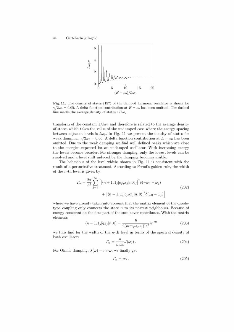
44 Gert-Ludwig Ingold
0 5 10 15 200
2
4
6
(E − ε0)/hω0
hω
0ρ
Fig. 11. The density of states (197) of the damped harmonic oscillator is shown forγ/2ω0 = 0.05. A delta function contribution at E = ε0 has been omitted. The dashedline marks the average density of states 1/~ω0
transform of the constant 1/~ω0 and therefore is related to the average densityof states which takes the value of the undamped case where the energy spacingbetween adjacent levels is ~ω0. In Fig. 11 we present the density of states forweak damping, γ/2ω0 = 0.05. A delta function contribution at E = ε0 has beenomitted. Due to the weak damping we find well defined peaks which are closeto the energies expected for an undamped oscillator. With increasing energythe levels become broader. For stronger damping, only the lowest levels can beresolved and a level shift induced by the damping becomes visible.
The behaviour of the level widths shown in Fig. 11 is consistent with theresult of a perturbative treatment. According to Fermi’s golden rule, the widthof the n-th level is given by
Γn =2π
~2
∞∑
j=1
[
∣
∣〈n+ 1, 1j|cjqxj |n, 0〉∣
∣
2δ(−ω0 − ωj)
+∣
∣〈n− 1, 1j|cjqxj |n, 0〉∣
∣
2δ(ω0 − ωj)
]
(202)
where we have already taken into account that the matrix element of the dipole-type coupling only connects the state n to its nearest neighbours. Because ofenergy conservation the first part of the sum never contributes. With the matrixelements
〈n− 1, 1j|qxj |n, 0〉 =~
2(mmjω0ωj)1/2n1/2 (203)
we thus find for the width of the n-th level in terms of the spectral density ofbath oscillators
Γn =n
mω0J(ω0) . (204)
For Ohmic damping, J(ω) = mγω, we finally get
Γn = nγ . (205)
Path Integrals and Quantum Dissipation 45
As observed before, the levels broaden with increasing damping strength γ andlevel number n. We remark that one can demonstrate by a semiclassical analysisof other one-dimensional potentials that it is indeed the level number and notthe energy which is decisive for the level width [37].
4.3 Position Autocorrelation Function
In the introduction we have mentioned fluctuations as one of the effects arisingfrom the coupling to an environment. Even if a system is in thermal equilibriumwith its environment, fluctuations due to the noise term (128) will be present.The appropriate quantity to describe this phenomenon are equilibrium correla-tion functions like the position autocorrelation function
C(t) = 〈q(t)q(0)〉 = Tr(q(t)q(0)ρβ) . (206)
From this quantity one can derive all other equilibrium correlation functions ofthe damped harmonic oscillator as is discussed in [38].
We now want to determine this correlation function by first calculating itsimaginary time version and start with the Euclidean action
SE[q] =
∫ ~β
0
dτ(m
2q2 +
m
2ω2
0q2)
+1
2
∫ ~β
0
dτ
∫ ~β
0
dσk(τ − σ)q(τ)q(σ)
+
∫
~β
0
dτF (τ)q(τ) .
(207)
The second term accounts for the coupling to the environment as we have shownin Sect. 3.3. In addition, we have included the third term corresponding to anexternal force in imaginary time. This constitutes a useful trick which will allowus to determine the correlation function by variation with respect to this force
〈q(τ)q(σ)〉 = ~2Tr
(
δ
δF (τ)
δ
δF (σ)ρ
)∣
∣
∣
∣
F=0
. (208)
As we know already from Sect. 2.7, the force does not appear in the fluctua-tion part. It is therefore sufficient, to restrict our attention to the classical path.The classical equation of motion following from variation of the action (207)
mq(τ) −∫ ~β
0
dσk(τ − σ)q(σ) −mω20q(τ) = F (τ) (209)
is most conveniently solved by Fourier transformation on the interval from 0 to~β. Introducing the Fourier transforms
q(τ) =1
~β
∞∑
n=−∞
qn exp(iνnτ) (210)
and
F (τ) =m
~β
∞∑
n=−∞
fn exp(iνnτ) (211)
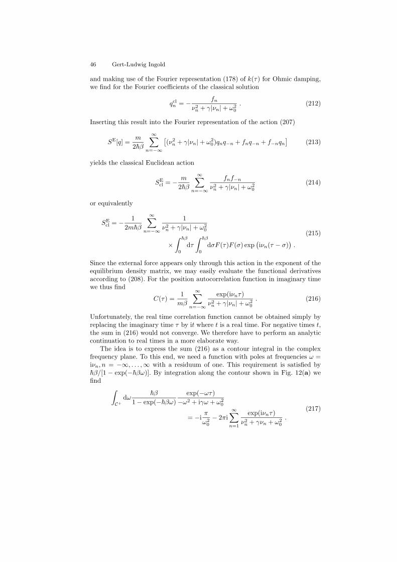
46 Gert-Ludwig Ingold
and making use of the Fourier representation (178) of k(τ) for Ohmic damping,we find for the Fourier coefficients of the classical solution
qcln = − fn
ν2n + γ|νn| + ω2
0
. (212)
Inserting this result into the Fourier representation of the action (207)
SE[q] =m
2~β
∞∑
n=−∞
[
(ν2n + γ|νn| + ω2
0)qnq−n + fnq−n + f−nqn]
(213)
yields the classical Euclidean action
SEcl = − m
2~β
∞∑
n=−∞
fnf−n
ν2n + γ|νn| + ω2
0
(214)
or equivalently
SEcl = − 1
2m~β
∞∑
n=−∞
1
ν2n + γ|νn| + ω2
0
×∫ ~β
0
dτ
∫ ~β
0
dσF (τ)F (σ) exp(
iνn(τ − σ))
.
(215)
Since the external force appears only through this action in the exponent of theequilibrium density matrix, we may easily evaluate the functional derivativesaccording to (208). For the position autocorrelation function in imaginary timewe thus find
C(τ) =1
mβ
∞∑
n=−∞
exp(iνnτ)
ν2n + γ|νn| + ω2
0
. (216)
Unfortunately, the real time correlation function cannot be obtained simply byreplacing the imaginary time τ by it where t is a real time. For negative times t,the sum in (216) would not converge. We therefore have to perform an analyticcontinuation to real times in a more elaborate way.
The idea is to express the sum (216) as a contour integral in the complexfrequency plane. To this end, we need a function with poles at frequencies ω =iνn, n = −∞, . . . ,∞ with a residuum of one. This requirement is satisfied by~β/[1 − exp(−~βω)]. By integration along the contour shown in Fig. 12(a) wefind
∫
C+
dω~β
1 − exp(−~βω)
exp(−ωτ)−ω2 + iγω + ω2
0
= −iπ
ω20
− 2πi
∞∑
n=1
exp(iνnτ)
ν2n + γνn + ω2
0
.
(217)
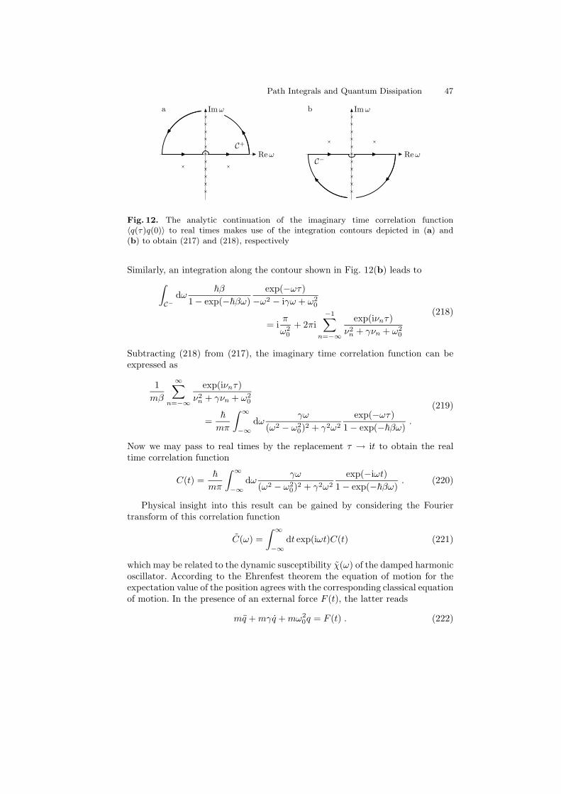
Path Integrals and Quantum Dissipation 47
Reω
Imωa
C+
Reω
Imωb
C−
Fig. 12. The analytic continuation of the imaginary time correlation function〈q(τ )q(0)〉 to real times makes use of the integration contours depicted in (a) and(b) to obtain (217) and (218), respectively
Similarly, an integration along the contour shown in Fig. 12(b) leads to
∫
C−
dω~β
1 − exp(−~βω)
exp(−ωτ)−ω2 − iγω + ω2
0
= iπ
ω20
+ 2πi
−1∑
n=−∞
exp(iνnτ)
ν2n + γνn + ω2
0
(218)
Subtracting (218) from (217), the imaginary time correlation function can beexpressed as
1
mβ
∞∑
n=−∞
exp(iνnτ)
ν2n + γνn + ω2
0
=~
mπ
∫ ∞
−∞
dωγω
(ω2 − ω20)
2 + γ2ω2
exp(−ωτ)1 − exp(−~βω)
.
(219)
Now we may pass to real times by the replacement τ → it to obtain the realtime correlation function
C(t) =~
mπ
∫ ∞
−∞
dωγω
(ω2 − ω20)
2 + γ2ω2
exp(−iωt)
1 − exp(−~βω). (220)
Physical insight into this result can be gained by considering the Fouriertransform of this correlation function
C(ω) =
∫ ∞
−∞
dt exp(iωt)C(t) (221)
which may be related to the dynamic susceptibility χ(ω) of the damped harmonicoscillator. According to the Ehrenfest theorem the equation of motion for theexpectation value of the position agrees with the corresponding classical equationof motion. In the presence of an external force F (t), the latter reads
mq +mγq +mω20q = F (t) . (222)
48 Gert-Ludwig Ingold
The solution of this equation may be expressed in terms of the response functionχ(t) as
q(t) =
∫ t
−∞
dsχ(t− s)F (s) (223)
which by means of a Fourier transformation becomes
q(ω) = χ(ω)F (ω) . (224)
With the equation of motion (222) the dynamic susceptibility of the dampedharmonic oscillator is then found to read
χ(ω) =1
m
1
−ω2 − iγω + ω20
. (225)
Together with (220) and (221) one finally obtains the relation
C(ω) =2~
1 − exp(−~βω)χ′′(ω) (226)
which represents an example of the so-called fluctuation-dissipation theorem[39]. Here, the position autocorrelation function describes the fluctuations whilethe imaginary part of the dynamic susceptibility χ′′ can be shown to determinethe energy dissipated under the influence of the external driving F (t). Whilethe relation (226) is exact for linear systems like the damped harmonic oscilla-tor considered here, it still holds for nonlinear systems within linear responsetheory. There, the response to the external force is considered in leading orderperturbation theory [40,41].
It is instructive to consider the real time correlation function (220) in moredetail. We first decompose the correlation function C(t) into its real and imagi-nary part, or equivalently, into its symmetric and antisymmetric part
C(t) = S(t) + iA(t) , (227)
with
S(t) =1
2
(
〈q(t)q(0)〉 + 〈q(0)q(t)〉)
(228)
and
A(t) = − i
2
(
〈q(t)q(0)〉 − 〈q(0)q(t)〉)
. (229)
From (220) we find
S(t) =~
2πm
∫ ∞
−∞
dωγω
(ω2 − ω20)
2 + γ2ω2coth
(
~βω
2
)
cos(ωt) (230)
and
A(t) = − ~
2πm
∫ ∞
−∞
dωγω
(ω2 − ω20)
2 + γ2ω2sin(ωt) . (231)

Path Integrals and Quantum Dissipation 49
Apart from Planck’s constant appearing in the prefactor, the antisymmetric partis purely classical. In fact, one demonstrates within linear response theory thegeneral relation
χ(t) =i
~〈[q(t), q(0)]〉Θ(t) = −2
~A(t)Θ(t) . (232)
Therefore, our statement follows as a consequence of the Ehrenfest theoremwhich ensures that the response function χ(t) of the damped harmonic oscillatoris classical.
More interesting is the symmetric part (230) of the correlation function C(t).There exist two different types of time scales determined by the poles of theintegrand in (230). One set of four poles at frequencies
ω = ±(
ω ± iγ
2
)
(233)
corresponds to the characteristic frequencies of a damped harmonic oscillatorwith the oscillation frequency
ω =
(
ω20 − γ2
4
)1/2
(234)
shifted by the damping. In addition, there exists an infinite number of poles atimaginary frequencies iνn, n = −∞, . . . ,∞ depending on the temperature of theheat bath via the Matsubara frequencies defined in (107). With these poles, onecan evaluate the integral (230) by means of a contour integration to obtain
S(t) =~
2mωexp(−γ|t|/2)
[sinh(~βω) cos(ωt) + sin(~βγ/2) sin(ω|t|)]cosh(~βω) − cos(~βγ/2)
− 2γ
mβ
∞∑
n=1
νn exp(−νn|t|)(ν2
n + ω20)
2 − γ2ν2n
.
(235)
The sum in the second line becomes important at low temperatures kBT ≪~γ/4π. In order to discuss this quantum effect, we focus in the following discus-sion on the case of zero temperature. Then, the poles of the hyperbolic cotangentin (230) become dense and form a cut on the imaginary axis which has conse-quences for the long-time behaviour of the correlation function. In the limitβ → ∞ the sum in the second line of (235) turns into an integral. Noting thatthe long-time behaviour is determined by the behaviour of the integrand at smallarguments we find
S(t) ∼ − ~γ
πm
∫ ∞
0
dxx exp(−x|t|)
ω40
= − ~γ
πmω40
1
t2. (236)
Instead of the usual exponential decay we thus find an algebraic decay.In the limit of vanishing damping, the imaginary part of the dynamic suscep-
tibility appearing in the integrand of (230) turns into a sum of two delta functions

50 Gert-Ludwig Ingold
located at ω0 and −ω0. For weak but finite damping, the delta functions broadeninto Lorentzians
γω
(ω2 − ω20)
2 + γ2ω2=
γ
4ω
(
1
(ω − ω)2 + γ2/4− 1
(ω + ω)2 + γ2/4
)
(237)
corresponding to the four poles (233) and one can assume that only the integrandin the neighbourhood of these poles is relevant. Within the so-called Markov ap-proximation, one then replaces the contributions to the integrand which dependonly weakly on frequency by their values at ω. As we will see, in contrast to(236) the correlation function S(t) at zero temperature then no longer decaysalgebraically. It is interesting to discuss the reason for this discrepancy.
To this end we go back to the integral representation (230) of the correlationfunction S(t). In a first step, we apply the so-called rotating wave approximation(RWA) which consists in neglecting the Lorentzian located at −ω, i.e. the secondterm in (237) [42]. Physically speaking, we neglect processes where the systemis excited into an energetically higher state by loosing energy to the drivingforce or where the system decays to a lower state by absorbing energy. For finitetemperatures, we now have
SRWA(t) =~
8πmω
∫ ∞
−∞
dωγ
(ω − ω)2 + γ2/4coth
(
~βω
2
)
cos(ωt) . (238)
Within the Markov approximation, we replace the hyperbolic cotangent by itsvalue at ω = ω. In the limit of zero temperature this leads to
SRWA,Markov(t) =~
8πmω
∫ ∞
−∞
dωγ
(ω − ω)2 + γ2/4cos(ωt)
=~
4mωcos(ωt) exp
(
−γ2t)
.
(239)
We thus find an oscillation with a frequency shifted due to the environmentalcoupling and an exponential decay in contrast to the algebraic decay (236).
This difference can be understood by taking a closer look at the Markov ap-proximation. In Fig. 13 the Lorentzian and the hyperbolic cotangent appearingin (238) are schematically shown as full and dashed line, respectively. In orderto obtain (239), we have approximated the hyperbolic cotangent by a constant.However, in doing this, we have replaced an antisymmetric function by a sym-metric one which can only yield a non-vanishing result together with the rotatingwave approximation made above. As a consequence, the area shaded in grey hasbeen taken with the wrong sign. The idea was that this difference should besmall and arising from frequencies far from ω. However, due to the large extentof a Lorentzian, it is of order γ and, in addition, it replaces an exponential decayby an algebraic decay.
At zero temperature the difference between (238) and (239) becomes
∆ = SRWA(t) − SRWA,Markov(t)
= −2~
8πm
∫ 0
−∞
dωγ
(ω − ω)2 + γ2/4cos(ωt)
(240)

Path Integrals and Quantum Dissipation 51
ω
Fig. 13. The full and dashed lines represent the Lorentzian and hyperbolic cotangent,respectively, which contribute to the integrand in (238)
which may be expressed in terms of integral sine and integral cosine functions.For our purpose it is sufficient to note that for long times, the difference indeeddecays algebraically as
∆ = − ~γ
2πmω40
1
t2. (241)
We remark that the factor of two relative to the result (236) arises because norotating wave approximation has been made in deriving the latter.
In the previous discussion, we have been concerned with an effect of orderγ which in the spirit of the Markov approximation should be considered assmall. However, the Markov approximation changes the long-time behaviour ofthe equilibrium correlation function S(t) qualitatively and the absence of analgebraic decay, even with a small prefactor, may be relevant. For truly weakcoupling, the damping constant γ should be the smallest frequency scale. Apartfrom the usual weak coupling condition γ ≪ ω0 we also have to require γ ≪kBT/~ which at low temperatures may become difficult to satisfy.
Acknowledgment
This chapter is based on courses taught at the Max-Planck-Institut fur Physikkomplexer Systeme in Dresden and at the Universite Louis Pasteur Strasbourg.The author is grateful to the organizers of the school on “Coherent evolutionin noisy environments”, in particular Andreas Buchleitner (Dresden), as wellas Rodolfo Jalabert (ULP Strasbourg) for having provided the opportunity tolecture on path integrals and quantum dissipation. The participants of the twocourses through their questions contributed to these lecture notes. It is a plea-sure to acknowledge inspiring conversations with Giovanna Morigi which havemotivated some of the discussions in particular in the last section. Furthermore,I am indebted to Peter Hanggi for several useful comments on an earlier versionof the manuscript and for drawing my attention to some less known references.
52 Gert-Ludwig Ingold
References
1. U. Weiss: Quantum Dissipative Systems (World Scientific 1999)2. T. Dittrich, P. Hanggi, G.-L. Ingold, B. Kramer, G. Schon, W. Zwerger: Quantum
transport and dissipation (Wiley-VCH 1998)3. H. Kleinert: Path Integrals in Quantum Mechanics, Statistics and Polymer Physics
(World Scientific 1995)4. R. P. Feynman: Rev. Mod. Phys. 20, 367 (1948)5. For a few historical remarks see e.g. D. Derbes: Am. J. Phys. 64, 881 (1996)6. P. A. M. Dirac: Phys. Zs. Sowjetunion 3, 64 (1933)7. see e.g. E. Nelson, J. Math. Phys. 5, 332 (1964), Appendix B8. F. Langouche, D. Roekaerts, E. Tirapegui: Functional Integration and Semiclas-
sical Expansions, Mathematics and Its Applications Vol. 10 (D. Reidel 1982)9. W. Janke, H. Kleinert: Lett. Nuovo Cim. 25, 297 (1979)
10. M. Goodman: Am. J. Phys. 49, 843 (1981)11. A. Auerbach, L. S. Schulman: J. Phys. A 30, 5993 (1997)12. I. S. Gradshteyn, I. M. Rhyzik: Table of Integrals, Series, and Products (Academic
Press 1980)13. V. P. Maslov, M. V. Fedoriuk: Semi-classical approximation in quantum mechan-
ics, Mathematical Physics and Applied Mathematics Vol. 7, ed. by M. Flato et al.(D. Reidel 1981)
14. P. A. Horvathy: Int. J. Theor. Phys. 18, 245 (1979)15. D. Rohrlich: Phys. Lett. A 128, 307 (1988)16. M. S. Marinov: Phys. Rep. 60, 1 (1980), Chap. 3.317. see e.g. M. Brack, R. K. Bhaduri: Semiclassical Physics, Frontiers in Physics Vol.
96 (Addison-Wesley 1997)18. J. H. van Vleck: Proc. Natl. Acad. Sci. USA 14, 178 (1928)19. C. Morette: Phys. Rev. 81, 848 (1951)20. W. Pauli: Selected Topics in Field Quantization, Pauli Lectures on Physics Vol. 6,
ed. by C. P. Enz (Dover 2000)21. N. Wiener: J. Math. Phys. M.I.T. 2, 131 (1923)22. A. O. Caldeira, A. J. Leggett: Phys. Rev. Lett. 46, 211 (1981)23. A. O. Caldeira, A. J. Leggett: Ann. Phys. (N.Y.) 149, 374 (1983)24. V. B. Magalinskiı: Zh. Eksp. Teor. Fiz. 36, 1942 (1959) [Sov. Phys. JETP 9, 1381
(1959)]25. I. R. Senitzky: Phys. Rev. 119, 670 (1960); 124, 642 (1961)26. G. W. Ford, M. Kac, P. Mazur: J. Math. Phys. 6, 504 (1965)27. P. Ullersma: Physica 32, 27, 56, 74, 90 (1966)28. R. Zwanzig: J. Stat. Phys. 9, 215 (1973)29. P. C. Hemmer, L. C. Maximon, H. Wergeland: Phys. Rev. 111, 689 (1958)30. P. Hanggi: ‘Generalized Langevin Equations: A Useful Tool for the Perplexed
Modeller of Nonequilibrium Fluctuations?’. In: Lecture Notes in Physics Vol. 484,ed. by L. Schimansky-Geier, T. Poschel (Springer 1997) pp. 15–22
31. V. Hakim, V. Ambegaokar: Phys. Rev. A 32, 423 (1985)32. H. Grabert, P. Schramm, G.-L. Ingold: Phys. Rev. Lett. 58, 1285 (1987)33. R. P. Feynman, F. L. Vernon, Jr.: Ann. Phys. (N.Y.) 24, 118 (1963)34. H. Grabert, P. Schramm, G.-L. Ingold: Phys. Rep. 168, 115 (1988)35. A. Hanke, W. Zwerger: Phys. Rev. E 52, 6875 (1995)36. M. Abramowitz, I. A. Stegun (eds.): Handbook of mathematical functions (Dover
1972)
Path Integrals and Quantum Dissipation 53
37. G.-L. Ingold, R. A. Jalabert, K. Richter: Am. J. Phys. 69, 201 (2001)38. H. Grabert, U. Weiss, P. Talkner: Z. Phys. B 55, 87 (1984)39. H. B. Callen, T. A. Welton: Phys. Rev. 83, 34 (1951)40. R. Kubo: J. Phys. Soc. Japan 12, 570 (1957)41. R. Kubo: Rep. Progr. Phys. 29, 255 (1966)42. R. Loudon: The Quantum Theory of Light (Oxford University Press 1983)