Detecting intraday periodicities with application to high ... · 2006 Royal Statistical Society...

2006 Royal Statistical Society 0035–9254/06/55241

Appl. Statist. (2006)55, Part 2, pp. 241–259

Detecting intraday periodicities with applicationto high frequency exchange rates

Chris Brooks

Cass Business School, London, UK

and Melvin J. Hinich

University of Texas at Austin, USA

[Received February 2003. Final revision August 2003]

Summary. Many recent papers have documented periodicities in returns, return volatility, bid–ask spreads and trading volume, in both equity and foreign exchange markets. We proposeand employ a new test for detecting subtle periodicities in time series data based on a signalcoherence function.The technique is applied to a set of seven half-hourly exchange rate series.Overall, we find the signal coherence to be maximal at the 8-h and 12-h frequencies. Retainingonly the most coherent frequencies for each series, we implement a trading rule that is basedon these observed periodicities. Our results demonstrate in all cases except one that, in grossterms, the rules can generate returns that are considerably greater than those of a buy-and-holdstrategy, although they cannot retain their profitability net of transactions costs. We conjecturethat this methodology could constitute an important tool for financial market researchers whichwill enable them to detect, quantify and rank the various periodic components in financial databetter.

Keywords: Exchange rates; Forecasting; Periodicities; Seasonality; Spectral analysis; Tradingrules

1. Introduction

Many recent papers have documented periodicities in returns, return volatility, bid–ask spreadsand trading volume, in both equity and foreign exchange markets. Such systematically recur-ring features or regularities have sometimes been termed calendar anomalies or seasonal effects.Examples include open and close effects, lunch-time effects, day of the week effects and holidayeffects. Studies of day of the week effects include French (1980), Gibbons and Hess (1981) andKeim and Stambaugh (1984), for example, all of whom have found that the average marketclose-to-close return in the USA is significantly negative on Monday and significantly positiveon Friday. Moreover, Rogalski (1984) and Smirlock and Starks (1986) observed that this neg-ative return between the Friday close and Monday close for the Dow–Jones industrial averageoccurs on Monday itself during the 1960s but moves backwards to the period between the Fridayclose and Monday opening in the late 1970s. By contrast, Jaffe and Westerfield (1985) foundthat the lowest mean returns for the Japanese and Australian stock-markets occur on Tuesdays.Harris (1986) also examined weekly and intraday patterns in stock returns and found that mostof the observed day of the week effects occur immediately after the opening of the market, witha price drop on Mondays on average at this time and rises on all other weekdays.

Address for correspondence: Chris Brooks, Faculty of Finance, Cass Business School, 106 Bunhill Row,London, EC1Y 8TZ, UK.E-mail: [email protected]

242 C. Brooks and M. J. Hinich

Recent research has also exploited the increasing availability of very high frequency and tickdata together with more powerful computational abilities to analyse more closely the intradaypatterns in financial markets. Wood et al. (1985) examined minute-by-minute returns data for alarge sample of New York Stock Exchange stocks. They found that significantly positive returnsare on average earned during the first 30 min of trading and at the market close, a result whichwas echoed by Ding and Lau (2001) using a sample of 200 stocks from the Stock Exchange ofSingapore. Andersen and Bollerslev (1997a) showed that the return volatility of the Germanmark–dollar exchange rate exhibits the same general intraday pattern as trading volume andbid–ask spreads. Using the same set of data, Andersen and Bollerslev (1998) also studied theeffects of macroeconomic announcements on the behaviour of the series. (An extensive surveyof the literature on intraday and intraweek seasonalities in stock-market indices and futuresmarket contracts is given in Yadav and Pope (1992).)

Such periodicities have typically been reconciled with the efficient markets hypothesis byappealing to market microstructure arguments (e.g. cyclical variations in market depth orliquidity, price discovery and inventory management), arrival of information, macroeconomicannouncements or tax effects. Many theoretical models of investor and market behaviour havealso been proposed to explain these stylized features of many financial time series, includingthose that account for the strategic behaviour of liquidity traders and informed traders (see,for example, Admati and Pfleiderer (1988). An alternative method for reconciling a finding ofrecurring seasonal patterns in financial markets is the possible existence of time-varying riskpremia, implying that expected returns need not be constant over time and could vary in partsystematically without implying market inefficiency.

Traditionally, studies that are concerned with the detection of periodicities in financial timeseries would either use a regression model with seasonal dummy variables (e.g. Chan et al.(1995)) or would apply spectral analysis to the sample of data (e.g. Bertoneche (1979) andUpson (1972)). Spectral analysis may be defined as a process whereby a series is decomposedinto a set of mutually orthogonal cyclical components of different frequencies. Calculating thespectrum involves fitting by least squares a set of sinusoidal curves, which is equivalent to aregression with trigonometric transformations of the independent variable. The spectrum, aplot of the signal amplitude against the frequency, will be flat for a white noise process, andevidence of periodic behaviour is indicated by statistically significant amplitudes at any givenfrequency. By examining the spectrum, Upson (1972) observed periodicities representing cyclesof duration 32, 3.8 and 2.5 weeks in US dollar–British pound data for the 1960s, whereas Ber-toneche (1979) could not detect any significant departures from randomness in an applicationof spectral analysis to a set of weekly European stock returns. Spectral analysis was a populartool for data analysis in economics and finance in the 1960s and 1970s (see also Granger (1966),Granger and Hatanaka (1964) and Granger and Morgenstern (1963)), although it has beenlargely discarded in the empirical economics and finance literature more recently. This seems tostem partly from the perceived inability of the spectral methods that were previously availableto detect the relevant temporal dependences in financial time series data.

In this paper, we propose and employ a new test for detecting periodicities in financial marketsbased on a signal coherence function. Our approach can be applied to any fairly large, evenlyspaced sample of time series data that is thought to contain periodicities. A periodic signalcan be predicted infinitely far into the future since it repeats exactly in every period. In fact, ineconomics and finance as in nature, there are no truly deterministic signals and hence there isalways some variation in the waveform over time. The notion of partial signal coherence, whichis developed in this paper into a statistical model, is a measure of how much the waveform var-ies over time. The coherence measures that are calculated are then employed to hone in on the

Intraday Periodicities 243

frequency components of the Fourier transforms of the signal that are the most stable over time.By retaining only those frequency components displaying the least variation over time, we candetect the most important seasonalities in the data, and these are then used to derive a tradingrule for buying or selling a currency in a hold-out sample. The performance of the trading ruleis then compared with that of buy-and-hold and randomized trading strategies. Our approachcan capture a much broader range of regularities than a linear regression with time-dependentdummy variables. The model that we propose based on the signal coherence function has beenshown to provide additional detectability relative to a Fisher test (see Hinich (2003)).

The remainder of this paper is organized as follows. Section 2 introduces some notationand defines the test statistics that are employed to detect the periodicities, whereas Section 3describes the data. Section 4 presents and analyses the results whereas Section 5 concludes andoffers suggestions for extensions and further research.

2. Methodology

2.1. Development of a test for signal autocoherenceThis paper develops below a model for a signal with randomly modulated periodicity, and ameasure known as a signal coherence function, which embodies the amount of random var-iation in each Fourier component of the signal. Let {x.tn/, n = 0, 1, 2, . . .} be a time series ofinterest sampled at equally spaced times t = nδ. The series would be said to exhibit randomlymodulated periodicity with period T if it is of the form

x.t/= a0

K+ 1

K

K∑k=1

{a1k +u1k.t/} cos.2πfkt/+ 1K

K∑k=1

{a2k +u2k.t/} sin.2πfkt/ .1/

where fk =k=T are called Fourier frequencies and K=T=δ. The uik.i=1, 2/ are jointly dependentzero-mean random processes that are periodic block stationary and satisfy finite dependence.The modulations are in the fundamental and harmonic frequency components and so a0 is aconstant. Note that we do not require u1k.tn/ and u2k.tn/ to be Gaussian. It is apparent fromequation (1) that the random variation occurs in the modulation rather than being additivenoise; in statistical parlance, the specification in equation (1) would be termed a random-effectsmodel. The modulations are produced by the data-generating mechanism and may be deter-ministic but in most cases the statistician analysing the data does not know the modulationsprocess and thus they are treated as random processes. The signal x.tn/ can be expressed as thesum of a deterministic (periodic) component and a stochastic process term:

x.t/= a0

K+ 1

K

K∑k=1

ak exp.2πifkt/+ 1K

K∑k=1

uk.t/ exp.2πifkt/ .2/

where ak =a1k − ia2k and uk.tn/=u1k.tn/− iu2k.tn/. The task at hand then becomes one of quan-tifying the relative magnitude of the kth modulations to the magnitude of the fixed effect ak foreach k.

A common approach to processing signals with a periodic structure is to portion the obser-vations into M frames, each of length T = Nδ, so that there is exactly one waveform in eachsampling frame. There could alternatively be an integer multiple of T observations in each frame.The periodic component of a.t/ is the mean component of x.t/. To determine how stable thesignal is at each frequency across the frames, the notion of signal coherence is employed. Signalcoherence is loosely analogous to the standard R2-measure that is used in regression analysisand quantifies the degree of association between two components for each given frequency. It


is worth noting that the methodology that we propose here is based on the coherence of the sig-nal across the frames for a single time series (which may also be termed autocoherence). This isquite different from the tests for signal coherence across markets that were used, for example, byHilliard (1979) and Smith (1999). (Both employed the frequency domain approach to examinethe extent to which stock-markets co-move across countries. Our technique is also distinct fromthat proposed by Durlauf (1991) and used by Fong and Ouliaris (1995) to detect departures froma random walk in five weekly US dollar exchange rate series. Both Fong and Ouliaris (1995)and Andersen and Bollerslev (1997a) detected long memory effects in the currency rates.)

The discrete Fourier transform of the mth frame, beginning at observation βm = .m−1/T +δand ending at observation mT for frequency fk =k=T , is given by

xm.k/=T−δ∑t=0

x.βm + t/ exp.−2πifkt/

=ak +Um.k/ .3/

where

Um.k/=T−δ∑t=0

u.βm + t/ exp.−2πifkt/:

The variance of Um.k/ is given by

σ2u.k/=

T−δ∑τ=0

exp.−2πifkτ /T−τ−1∑

t=0cu.t, t + τ / .4/

where cu.t1, t2/ = E{uÅm.t1/ um.t2/}, and the variance is of order O.T/. Provided that um.tn/ is

weakly stationary, equation (4) can be written as

σ2u.k/=T {Su.fk/+O.1=T/} .5/

where Su.f/ is the spectrum of u.tn/.Although the model for randomly modulated periodicity is not in general a cyclostationary

model, when the assumption of weak stationarity is added, it becomes so (see Gladyshev (1961),Gardner and Franks (1975) and Gardner (1985, 1994) for extensive writings on cyclostation-arity). The signal coherence function γx.k/ measures the variability of the signal across theframes and is defined as follows for each frequency fk:

γx.k/=√{ |ak|2

|ak|2 +σ2u.k/

}: .6/

It is obvious from the construction of γx.k/ in equation (6) that it is bounded to lie on the interval[0,1]. The end point case γx.k/=1 will occur if ak �=0 and σ2

u.k/=0, which is the case where thesignal component at frequency fk has a constant amplitude and phase over time, so that thereis no random variation across the frames at that frequency (perfect coherence). The other endpoint, γx.k/ = 0, will occur if ak = 0 and σ2

u.k/ �= 0, when the mean value of the component atfrequency fk is 0, so that all of the variation across the frames at that frequency is pure noise(no coherence).

The signal coherence function is estimated from the actual data by taking the Fourier trans-form of the mean frame and for each of the M frames. The mean frame will be given by

x.tn/= 1M

M∑m=1

x.βm + tn/, n=0, 1, . . . , N −1: .7/


Letting a.k/ denote the mean frame estimate, with its Fourier transform being A.k/, and lettingXm.k/ denote the Fourier transform for the mth frame, then Dm.k/=Xm.k/− A.k/ is a measureof the difference between the Fourier transforms of the mth frame and the mean frame for eachfrequency. The signal coherence function can then be estimated by

γx.k/=√{ |Ak|2

|Ak|2 + .1=M/M∑

m=1|Dm.k/|2

}.8/

and 0� γx.k/�1. It can be shown (see Hinich (2000)) that the null hypothesis of zero coherenceat frequency fk can be tested by using the statistic M γx.k/2={1 − γx.k/2}, which is asymptot-ically distributed under the null hypothesis as a non-central χ2-distribution with 2 degrees offreedom and non-centrality parameter given by

λk =Ma2k=T Su.fk/,

where Su.fk/ is the spectrum of {u.t/} at the frequency fk. We also employ a joint test of the nullhypothesis that there is zero coherence across the M frames for all K=2 frequencies examined.This test statistic will asymptotically follow a non-central χ2-distribution with K degrees offreedom.

2.2. Development and testing of a trading ruleThe sample is split into (M =) 52 non-overlapping frames each of length 1 week, with eachweek of observations containing 240 half-hourly observations. (The choice of frame length isbound to be somewhat arbitrary, although in our case it represents a trade-off between havinga sufficient number of frames over which to compute the tests, while having a sufficiently longframe to detect interesting periodic components.) This implies that a total of 120 periodicitieswill be examined: 240, 120, 80, 60, 48, . . . , 240/119, 2, using the whole sample of data, andthe autocoherence measures are calculated across the 52 frames. Following initial exploratoryanalysis and estimation of the signal coherence function for the whole year’s set of frames data,the sample is then split into two portions. The first 26 weeks (6240 half-hourly observations) areused for in-sample estimation of the coherence function (across the resulting 26 frames), andthe remaining data are held back for out-of-sample trading rule evaluation. The out-of-sampleperiod begins with the return of 00:30 a.m.–01:00 a.m. on July 1st, 1996.

For the out-of-sample trading rule analysis, the signal coherence function is re-estimatedusing the first half of the sample only, and the mean frame is ‘cleaned’ by removing all fre-quency components with signals whose random variation implies that they are not statisticallycoherent at the 1% level of significance. Statistically, if Pr{γx.k/ = 0} < 0:01, ajk .j = 1, 2/ arekept; otherwise ajk are set to 0. The coherent part of the mean frame is analogous to the fittedvalue of the dependent value in a standard regression model. Retaining only the most coherentfrequencies for each series, we implement a trading rule that is based on these observed peri-odicities, ‘buying’ the foreign currency if the return is predicted to be positive and assuming noposition if it is predicted to be negative. The trading rule is then compared with a buy-and-holdthe foreign currency strategy and also in a novel way involving a simulation. To evaluate thestatistical significance of the strategies, we generate random binomial 0–1 draws equal in num-ber to the out-of-sample observations. This column of 0s and 1s is then multiplied by the actualreturn series and added over the hold-out sample to generate a profit from a randomized marketentry and exit rule. This is repeated 10000 times to generate a distribution of artificial rules andsubsequent artificial returns, which is then compared with the profit that is generated by the


rules that are based on the coherent periodic signal. If the actual rule generates a profit that islarger than 95% of those generated by artificial timing, it is considered to produce statisticallysignificant abnormal returns.

We then exploit the information that is contained in the lower half of the signal coherencefunction by short selling the foreign currency when it is periodically expected to exhibit negativereturns, as well as taking a long-term position when it is expected to yield positive returns. Therelevant simulation comparator is now one where the column of 0s and 1s is modified to a col-umn of −1 and 1 to be mutliplied by the actual returns to give a set of returns from randomizedlong- and short-term positions.

3. Data

The high frequency financial data that were provided by Olsen and Associates as part of theHFDF-96 package includes 25 exchange rate series sampled half-hourly for the whole of 1996,making a total of 17568 observations for each series. However, this series contains observationscorresponding to week-end periods when all the world’s exchanges simultaneously have virtu-ally no trading. This period is the time from 23:00 h Greenwich Mean Time (GMT) on Fridaywhen North American financial centres close until 23:00 h GMT on Sunday when Australasianmarkets open. The incorporation of such prices would lead to spurious zero returns and wouldpotentially render trading strategies which recommended a buy or sell at this time to be non-sensical. Removal of these week-end observations leaves 12575 observations for subsequentanalysis and forecasting.

We do not account for differences in the dates that different countries switch to daylightsaving time, since the effect of this 1-h difference is likely to be negligible as trading occursvirtually at all times at some destination around the world. Moreover, it is not clear how suchan adjustment could be made. This problem would be much more serious if we were examining,say, cross-correlations between equity returns for stocks on markets that were in different timezones. Such an approach appears to be consistent with the existing literature—for example,Andersen and Bollerslev (1997b) did not correct for bank-holiday effects. Finally, it is worthnoting that if asynchronous switches to daylight saving time did make a difference to our results,since it is not possible to create coherence, only to destroy it, the effect would be to render ourresults less strong than they otherwise would have been rather than to cause spurious findings.

The price series that are used are the average of the most recent best bid and best ask prices inthat half-hour interval and are transformed into a set of continuously compounded half-hourlypercentage returns in the standard fashion. The first observation in the sample correspondsto the period between 00:30 a.m. and 01:00 a.m. GMT on January 1st, 1996, whereas the lastcorresponds to 11:30 p.m.–midnight GMT on December 31st of the same year.

Of the 25 exchange rate series that were provided by Olsen, only seven are used in this study toavoid repetition, and for brevity. These are (using the usual mnemonic) DEM JPY, GBP DEM,GBP USD, USD CHF, USD DEM, USD ITL and USD JPY. These are all quoted as unitsof the second (foreign) currency per unit of the first (domestic) currency. For example, xxx yyywould be the units of yyy per unit of xxx. Hence a positive return implies that the number ofunits of the foreign currency yyy per unit of the domestic currency (xxx) has increased. Thiswould imply a profit for an investor whose domestic currency is xxx, but who had switched intoyyy at the start of the period and converted the terminal sum back at the end.

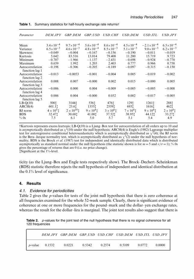
Some summary statistics for these seven returns series are presented in Table 1. It is clearly evi-dent that all series are non-normal (predominantly because of fat tails rather than asymmetry),and all exhibit evidence of negative first-order autocorrelation, and conditional heteroscedas-


Table 1. Summary statistics for half-hourly exchange rate returns†

Parameter DEM JPY GBP DEM GBP USD USD CHF USD DEM USD ITL USD JPY

Mean 3.4×10−4 9.7×10−4 5.6×10−4 8.6×10−4 4.5×10−4 −2.1×10−4 6.5×10−4

Variance 6.5×10−3 4.6×10−3 4.8×10−4 8.5×10−3 5.1×10−3 9.0×10−3 6.2×10−3

Skewness −0.049 −0.004 −0.167 −0.156 −0.190 −0.011 −0.019Kurtosis 5.642 83.516 13.014 79.408 11.200 15.719 9.723Minimum −0.707 −1.966 −1.137 −2.431 −0.698 −0.924 −0.770Maximum 0.659 1.992 1.203 2.403 0.777 0.966 0.758Autocorrelation −0.198 −0.306 −0.205 −0.189 −0.097 −0.315 −0.150

function lag 1Autocorrelation −0.013 −0.0053 −0.001 −0.004 0.005 −0.019 −0.002

function lag 2Autocorrelation 0.008 0.007 −0.000 0.002 0.015 −0.000 0.005

function lag 3Autocorrelation −0.006 0.000 0.004 −0.009 −0.005 −0.005 −0.008

function lag 4Autocorrelation 0.006 0.004 −0.000 0.032 0.002 −0.017 −0.005

function lag 5LB-Q(10) 500‡ 3144‡ 536‡ 476‡ 129‡ 1261‡ 288‡ARCH(4) 601.1‡ 23.6‡ 1355‡ 2559‡ 693‡ 1616‡ 462‡BJ norm 4×105‡ 2×1010‡ 9×104‡ 3×106‡ 7×104‡ 9×104‡ 2×104‡BDS 32.47‡ 30.68‡ 41.00‡ 37.52‡ 38.95‡ 44.12‡ 33.27‡% 0s 7.5 6.1 5.0 5.7 5.1 5.4 4.9

†Kurtosis represents excess kurtosis; LB-Q(10) is a Ljung–Box test for autocorrelation of all orders up to 10 andis asymptotically distributed as χ2(10) under the null hypothesis; ARCH(4) is Engle’s (1982) Lagrange multipliertest for autoregressive conditional heteroscedasticity which is asymptotically distributed as χ2(4); the BJ normis the Bera–Jarque normality test, which is asymptotically distributed as χ2(2) under the null hypothesis of nor-mality; BDS is the Brock et al. (1987) test for independent and identically distributed data which is distributedasymptotically as standard normal under the null hypothesis (the statistic shown is for m= 5 and "=σ = 1); % 0sgives the percentage of returns that are 0 (i.e. no price change).‡Significant at the 1%-level.

ticity (as the Ljung–Box and Engle tests respectively show). The Brock–Dechert–Scheinkman(BDS) statistic therefore rejects the null hypothesis of independent and identical distribution atthe 0.1% level of significance.

4. Results

4.1. Evidence for periodicitiesTable 2 gives the p-values for tests of the joint null hypothesis that there is zero coherence atall frequencies examined for the whole 52-week sample. Clearly, there is significant evidence ofcoherence at one or more frequencies for the pound–mark and the dollar–yen exchange rates,whereas the result for the dollar–lira is marginal. The joint test results also suggest that there is

Table 2. p-values for the joint test of the null hypothesis that there is no signal coherence for all120 frequencies

DEM JPY GBP DEM GBP USD USD CHF USD DEM USD ITL USD JPY

p-value 0.1532 0.0221 0.5342 0.2574 0.5109 0.0772 0.0000


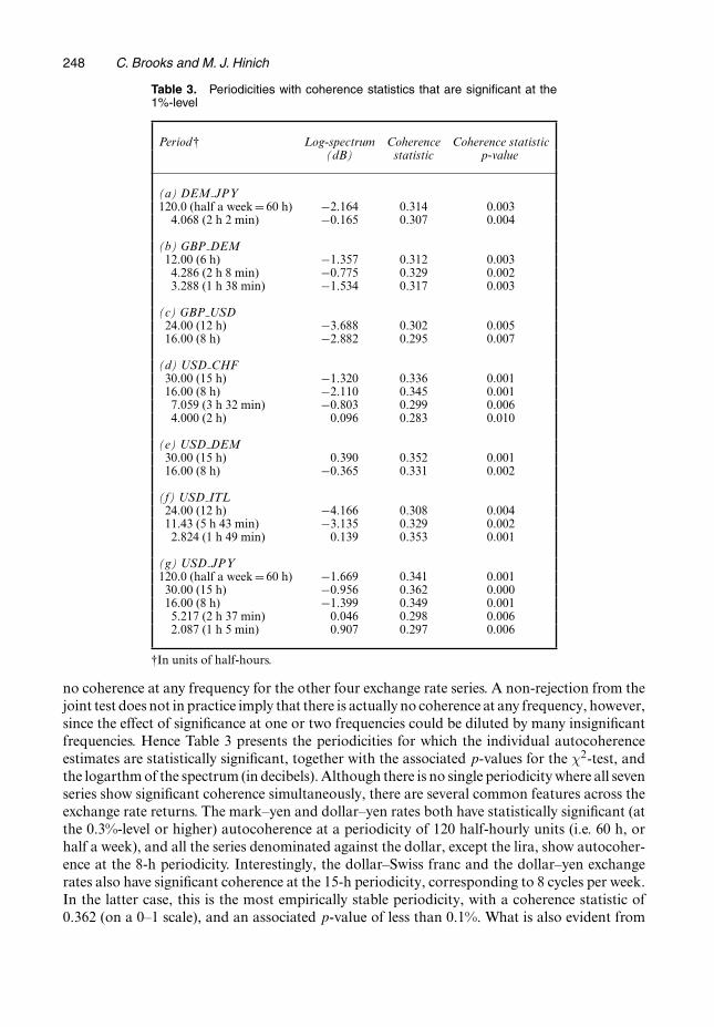
Table 3. Periodicities with coherence statistics that are significant at the1%-level

Period† Log-spectrum Coherence Coherence statistic(dB) statistic p-value

(a) DEM JPY120.0 (half a week=60 h) −2.164 0.314 0.003

4.068 (2 h 2 min) −0.165 0.307 0.004

(b) GBP DEM12.00 (6 h) −1.357 0.312 0.003

4.286 (2 h 8 min) −0.775 0.329 0.0023.288 (1 h 38 min) −1.534 0.317 0.003

(c) GBP USD24.00 (12 h) −3.688 0.302 0.00516.00 (8 h) −2.882 0.295 0.007

(d) USD CHF30.00 (15 h) −1.320 0.336 0.00116.00 (8 h) −2.110 0.345 0.001

7.059 (3 h 32 min) −0.803 0.299 0.0064.000 (2 h) 0.096 0.283 0.010

(e) USD DEM30.00 (15 h) 0.390 0.352 0.00116.00 (8 h) −0.365 0.331 0.002

(f) USD ITL24.00 (12 h) −4.166 0.308 0.00411.43 (5 h 43 min) −3.135 0.329 0.002

2.824 (1 h 49 min) 0.139 0.353 0.001

(g) USD JPY120.0 (half a week=60 h) −1.669 0.341 0.001

30.00 (15 h) −0.956 0.362 0.00016.00 (8 h) −1.399 0.349 0.001

5.217 (2 h 37 min) 0.046 0.298 0.0062.087 (1 h 5 min) 0.907 0.297 0.006

†In units of half-hours.

no coherence at any frequency for the other four exchange rate series. A non-rejection from thejoint test does not in practice imply that there is actually no coherence at any frequency, however,since the effect of significance at one or two frequencies could be diluted by many insignificantfrequencies. Hence Table 3 presents the periodicities for which the individual autocoherenceestimates are statistically significant, together with the associated p-values for the χ2-test, andthe logarthm of the spectrum (in decibels). Although there is no single periodicity where all sevenseries show significant coherence simultaneously, there are several common features across theexchange rate returns. The mark–yen and dollar–yen rates both have statistically significant (atthe 0.3%-level or higher) autocoherence at a periodicity of 120 half-hourly units (i.e. 60 h, orhalf a week), and all the series denominated against the dollar, except the lira, show autocoher-ence at the 8-h periodicity. Interestingly, the dollar–Swiss franc and the dollar–yen exchangerates also have significant coherence at the 15-h periodicity, corresponding to 8 cycles per week.In the latter case, this is the most empirically stable periodicity, with a coherence statistic of0.362 (on a 0–1 scale), and an associated p-value of less than 0.1%. What is also evident from


0

0.05

0.1

0.15

0.2

0.25

0.3

0.35

0.4

240 40

21.8 15

11.4

9.23

7.74

6.67

5.85

5.22

4.71

4.29

3.93

3.64

3.38

3.16

2.96

2.79

2.64 2.5

2.38

2.26

2.16

2.07

Period

Co

her

ence

U S D _JP Y

U S D _IT L

U S D _D EM

U S D _C H F

Fig. 1. Coherence against period for USD CHF, USD DEM, USD ITL and USD JPY

Fig. 2. Coherence against period for DEM JPY, GBP DEM and GBP USD

Table 3 is that none of the coherence statistics are larger than 0.362, implying that there is stilla considerable amount of variation in the waveform over the frames even for the most coherentparts. The log-spectrum in decibels is 20 times the natural logarithm of the spectral amplitude or,equivalently, it is 10 times the spectrum (in variance units). The measure in decibels, as shown inTable 3, gives on a log-scale the average sizes of the periodic movements in terms of the heightsof the peaks and troughs of the coherent periodicities. Whereas autocoherence quantifies howstable these periodicities are, the amplitude measures how big the cyclical fluctuations are. It isevident from the second column of Table 3 that, in general, the higher frequency components


–0.2

–0.15

–0.1

–0.05

0

0.05

0.1

0.15

0.2

1 10 19 28 37 46 55 64 73 82 91 100 109 118 127 136 145 154 163 172 181 190 199 208 217 226 235

Time

Ret

urn

Fig. 3. Coherent part of the mean frame for a week for DEM JPY

–0.2

–0.15

–0.1

–0.05

0

0.05

0.1

0.15

0.2

1 10 19 28 37 46 55 64 73 82 91 100 109 118 127 136 145 154 163 172 181 190 199 208 217 226 235

Time

Ret

urn

Fig. 4. Coherent part of the mean frame for a week for GBP DEM

have the largest amplitudes, with some even being positive (on a log-scale) at frequencies oflower than 3 h for the dollar–Swiss franc, dollar–lira and dollar–yen exchange rates.

How can we explain the observed 8-, 12- and 15-h periodicities? Several factors could justifytheir existence, including the opening and closing times of the three major markets in differenttime zones (London, New York and Japan), and related changes in market volatility and liquid-ity through each 24-h period. For example, Andersen and Bollerslev (1998), Fig. 3, reportedcycles in intraday volatility, where it is highest from 1 p.m. to 5 p.m., and lowest from 3 a.m.to 5 a.m. (GMT). It may therefore simply be that the cycles in returns are rewards for bearingtime-varying intradaily risks, which are themselves cyclical. A cycle that repeats every 8 h isconsistent with an effect that is driven by the opening and closing of the three markets, whereas


–0.15

–0.1

–0.05

0

0.05

0.1

0.15

1 10 19 28 37 46 55 64 73 82 91 100 109 118 127 136 145 154 163 172 181 190 199 208 217 226 235

Time

Ret

urn

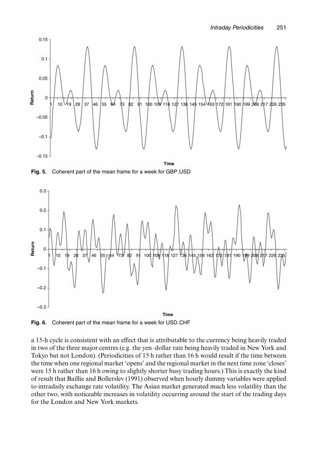
Fig. 5. Coherent part of the mean frame for a week for GBP USD

–0.3

–0.2

–0.1

0

0.1

0.2

0.3

1 10 19 28 37 46 55 64 73 82 91 100 109 118 127 136 145 154 163 172 181 190 199 208 217 226 235

Time

Ret

urn

Fig. 6. Coherent part of the mean frame for a week for USD CHF

a 15-h cycle is consistent with an effect that is attributable to the currency being heavily tradedin two of the three major centres (e.g. the yen–dollar rate being heavily traded in New York andTokyo but not London). (Periodicities of 15 h rather than 16 h would result if the time betweenthe time when one regional market ‘opens’ and the regional market in the next time zone ‘closes’were 15 h rather than 16 h owing to slightly shorter busy trading hours.) This is exactly the kindof result that Baillie and Bollerslev (1991) observed when hourly dummy variables were appliedto intradaily exchange rate volatility. The Asian market generated much less volatility than theother two, with noticeable increases in volatility occurring around the start of the trading daysfor the London and New York markets.


–0.15

–0.1

–0.05

0

0.05

0.1

0.15

1 10 19 28 37 46 55 64 73 82 91 100 109 118 127 136 145 154 163 172 181 190 199 208 217 226 235

Time

Ret

urn

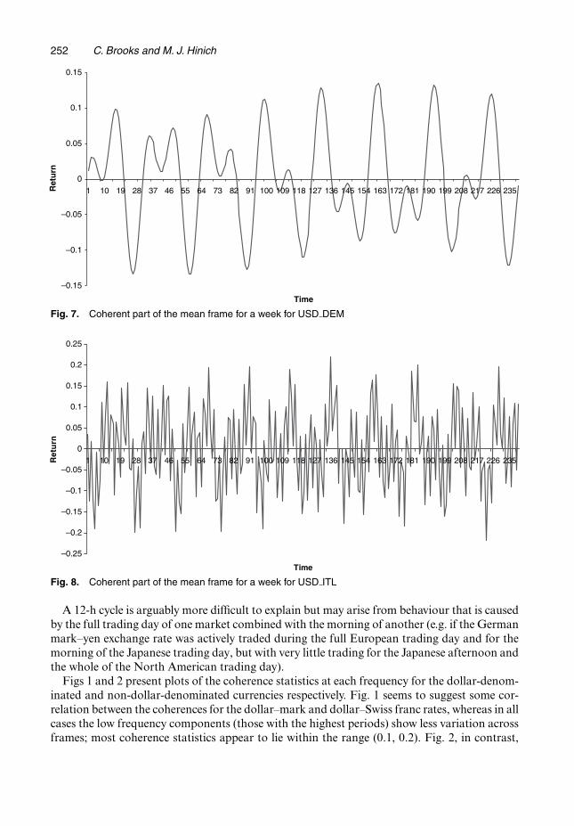
Fig. 7. Coherent part of the mean frame for a week for USD DEM

–0.25

–0.2

–0.15

–0.1

–0.05

0

0.05

0.1

0.15

0.2

0.25

1 10 19 28 37 46 55 64 73 82 91 100 109 118 127 136 145 154 163 172 181 190 199 208 217 226 235

Time

Ret

urn

Fig. 8. Coherent part of the mean frame for a week for USD ITL

A 12-h cycle is arguably more difficult to explain but may arise from behaviour that is causedby the full trading day of one market combined with the morning of another (e.g. if the Germanmark–yen exchange rate was actively traded during the full European trading day and for themorning of the Japanese trading day, but with very little trading for the Japanese afternoon andthe whole of the North American trading day).

Figs 1 and 2 present plots of the coherence statistics at each frequency for the dollar-denom-inated and non-dollar-denominated currencies respectively. Fig. 1 seems to suggest some cor-relation between the coherences for the dollar–mark and dollar–Swiss franc rates, whereas in allcases the low frequency components (those with the highest periods) show less variation acrossframes; most coherence statistics appear to lie within the range (0.1, 0.2). Fig. 2, in contrast,


–0.25

–0.2

–0.15

–0.1

–0.05

0

0.05

0.1

0.15

0.2

0.25

1 10 19 28 37 46 55 64 73 82 91 100 109 118 127 136 145 154 163 172 181 190 199 208 217 226 235

Time

Ret

urn

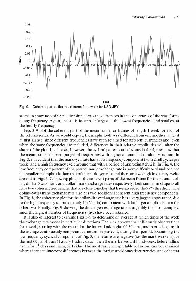
Fig. 9. Coherent part of the mean frame for a week for USD JPY

seems to show no visible relationship across the currencies in the coherences of the waveformsat any frequency. Again, the statistics appear largest at the lowest frequencies, and smallest atthe hourly frequency.

Figs 3–9 plot the coherent part of the mean frame for frames of length 1 week for each ofthe returns series. As we would expect, the graphs look very different from one another, at leastat first glance, since different frequencies have been retained for different currencies and, evenwhen the same frequencies are included, differences in their relative amplitudes will alter theshape of the plot. In all cases, however, the cyclical patterns are obvious in the figures now thatthe mean frame has been purged of frequencies with higher amounts of random variation. InFig. 3, it is evident that the mark–yen rate has a low frequency component (with 2 full cycles perweek) and a high frequency cycle around that with a period of approximately 2 h. In Fig. 4, thelow frequency component of the pound–mark exchange rate is more difficult to visualize sinceit is smaller in amplitude than that of the mark–yen rate and there are two high frequency cyclesaround it. Figs 5–7, showing plots of the coherent parts of the mean frame for the pound–dol-lar, dollar–Swiss franc and dollar–mark exchange rates respectively, look similar in shape as allhave two coherent frequencies that are close together that have exceeded the 99% threshold. Thedollar–Swiss franc exchange rate also has two additional coherent high frequency components.In Fig. 8, the coherence plot for the dollar–lira exchange rate has a very jagged appearance, dueto the high frequency (approximately 1 h 20 min) component with far larger amplitude than theother two. Finally, Fig. 9 showing the dollar–yen exchange rate is arguably the most complex,since the highest number of frequencies (five) have been retained.

It is also of interest to examine Figs 3–9 to determine on average at which times of the weekthe exchange rate moves in particular directions. The x-axis shows the half-hourly observationsfor a week, starting with the return for the interval midnight–00:30 a.m., and plotted against itthe average continuously compounded return, in per cent, during that period. Examining thelow frequency cyclical component of Fig. 3, the returns are negative (i.e. the mark weakens) forthe first 60 half-hours (1 and 1

4 trading days), then the mark rises until mid-week, before fallingagain for 1 1

4 days and rising on Friday. The most easily interpretable behaviour can be examinedwhere there are time-zone differences between the foreign and domestic currencies, and coherent


frequency components with periods of 8, 12 or 15 h, which there appears to be for many of theother series. For example, the pound–dollar exchange rate (Fig. 5) on average rises (the poundbecomes stronger) from the early hours of the morning GMT, until midday GMT, followedby falls when the US east coast markets start trading. The dollar–German mark exchange rateon average rises (the dollar strengthens) until around 10 a.m. GMT and then falls (the markstrengthens) while the European markets are open until 4 p.m. GMT, followed by further dollarappreciation. Similarly, the mark–Swiss franc exchange rate (Fig. 6) on average rises (the dollarstrengthens) until 10 a.m., with falls (the franc appreciates) until around 3 p.m., followed byfranc depreciation into the European evening. The dollar–yen exchange rate (Fig. 9) appears tofall (the dollar weakens) from midnight until 4 a.m. GMT, when the US markets are closed, andthen rises until around 2 p.m. GMT before falling back again. Finally, the dollar–lira exchangerate has such a large number of high frequency movements that any associations with marketopening and closing times are indiscernible.

These results support those of Ito and Roley (1987), who found a systematic dollar apprecia-tion against the yen during the US trading hours, and a systematic depreciation during Japanesetrading hours. Our results are also consistent with those of Baillie and Bollerslev (1991), whoobserved hourly patterns in foreign exchange market volatility related to major market openingand closing times. This is, perhaps, to be expected, since the weight of trading volume will movebetween the different world centres through the day.

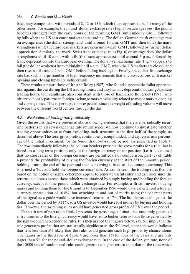
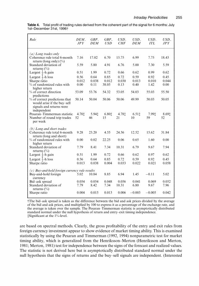
4.2. Evaluation of trading rule profitabilityGiven the results that were presented above showing evidence that there are periodically recur-ring patterns in all seven exchange rate return series, we now continue to investigate whethertrading opportunities arise from exploiting such structure in the first half of the sample, asdescribed above. The total gross profits, continuously compounded, and expressed as a percent-age of the initial investment, for the 6-month out-of-sample period, are presented in Table 4.The row immediately following the column headers presents the gross profits for a rule that isbased on a long-term position only in the foreign currency or no position (i.e. it is assumedthat no short sales of the foreign currency are permitted). For comparison, part (c) of Table4 presents the profitability of buying the foreign currency at the start of the 6-month period,holding it until the end of the year and then converting it back to the domestic currency. Thisis termed a ‘buy and hold the foreign currency’ rule. As can be seen, the trading rules that arebased on the notion of signal coherence appear to generate useful entry and exit rules since thereturns in all cases exceed those which were obtained by simply buying and holding the foreigncurrency, except for the pound–dollar exchange rate. For example, a British investor buyingmarks and holding them for the 6 months to December 1996 would have experienced a foreigncurrency appreciation of 10.8%, but switching in and out of marks using the coherent partsof the signal as a guide would have increased returns to 17%. The lira depreciated against thedollar over the period by 0.11%, so a US investor would have lost money by buying and holdinglira. However, the switching rules would have generated gross profits of 7.8% over the period.

The sixth row of part (a) in Table 4 presents the percentage of times that randomly generatedentry times into the foreign currency would have led to higher returns than those generated bythe signal-coherence-generated rules. It is then argued that figures below, say, 5% imply that therule generates profits that are statistically significant at the 5%-level, since this would indicatethat it is less than 5% likely that the rules could generate such high profits by chance alone.The figures in the third row of Table 4 are lower than 1% for four of the cases and are onlylarger than 5% for the pound–dollar exchange rate. In the case of the dollar–yen rate, none ofthe 10000 sets of randomized rules could generate a higher return than that of the rules which


Table 4. Total profit of trading rules derived from the coherent part of the signal for 6 months: July1st–December 31st, 1996†

Rule DEM GBP GBP USD USD USD USDJPY DEM USD CHF DEM ITL JPY

(a) Long trades onlyCoherence rule total 6-month 7.16 17.02 6.70 15.75 6.99 7.75 18.43

return (long only) (%)Standard deviation of 5.59 5.80 4.91 6.76 5.00 7.30 5.59

returns (%)Largest 1

2 -h gain 0.51 1.99 0.72 0.66 0.62 0.99 0.62Largest 1

2 -h loss 0.56 0.64 0.85 0.72 0.59 0.92 0.45Sharpe ratio 0.012 0.038 0.012 0.030 0.013 0.010 0.044% of randomized rules with 0.00 0.11 38.05 0.13 0.40 1.42 0.00

higher return% of correct direction 53.09 53.76 54.32 53.05 54.03 55.03 55.50

predictions% of correct predictions that 50.14 50.04 50.06 50.06 49.99 50.03 50.05

would arise if the buy–sellsignals and returns wereindependent

Pesaran–Timmerman statistic 4.70‡ 5.94‡ 6.80‡ 4.78‡ 6.51‡ 7.99‡ 8.69‡Number of round trip trades 52 46 15 21 10 59 52

per week

(b) Long and short tradesCoherence rule total 6-month 9.28 23.20 4.55 24.56 12.52 15.62 31.84

return (long and short)% of randomized rules with 0.00 0.02 22.25 0.06 0.65 1.60 0.00

higher returnStandard deviation of 7.79 8.41 7.34 10.31 6.79 9.67 7.94

returns (%)Largest 1

2 -h gain 0.51 1.99 0.72 0.66 0.62 0.97 0.62Largest 1

2 -h loss 0.56 0.64 0.85 0.72 0.59 0.92 0.45Sharpe ratio 0.013 0.038 0.004 0.033 0.022 0.021 0.058

(c) Buy-and-hold foreign currency rule resultsBuy-and-hold foreign 5.02 10.84 8.85 6.94 1.45 −0.11 5.02

currencyBid–ask spread 0.054 0.054 0.048 0.056 0.041 0.069 0.052Standard deviation of 7.79 8.42 7.34 10.31 6.80 9.67 7.96

returns (%)Sharpe ratio 0.004 0.015 0.013 0.006 −0.003 −0.005 0.042

†The bid–ask spread is taken as the difference between the bid and ask prices divided by the averageof the bid and ask prices, and multiplied by 100 to express it as a percentage of the exchange rate, andthe average is taken over the sample. The Pesaran–Timmerman statistic is asymptotically distributedstandard normal under the null hypothesis of return and entry–exit timing independence.‡Significant at the 1%-level.

are based on spectral methods. Clearly, the gross profitability of the entry and exit rules fromforeign currency investment appear to show evidence of market timing ability. This is examinedstatistically by using the Pesaran and Timmerman (1992, 1994) nonparametric test for markettiming ability, which is generalized from the Henriksson–Merton (Henriksson and Merton,1981; Merton, 1981) test for independence between the signs of the forecast and realized values.The statistic is not derived here but is asymptotically distributed standard normal under thenull hypothesis that the signs of returns and the buy–sell signals are independent. (Interested


readers are referred to Pesaran and Timmerman (1992, 1994), Henriksson and Merton (1981)and Merton (1981) for a derivation of the test statistic.) The number of correct sign predictionsvaries between 53% and 55% across the currencies, whereas the number of correct predictionsthat would be expected to result if the buy–sell signals and actual returns were independentis very close to 50% in all cases. Note that the use of very high frequency data implies that anon-negligible number of actual returns per half-hour interval are 0. Although it is not clearfrom an examination of the formulation of the test, we define zero returns as implying correctsign predictions if the rule signal for that observation had been a 0 (so that the transactions coststhat are associated with buying the foreign currency are correctly avoided). However, incorrectsign predictions are argued to result if the rule generated no buy signal, but the return turnedout to be positive. The relatively high proportion of correct sign predictions combined withthe large sample size leads the Pesaran–Timmerman statistic to reject the null hypothesis at the1%-level convincingly in all cases.

The trading profitability of rules exploiting the sell signals that were generated for those obser-vations when the coherence plots are negative are also examined in part (b) of Table 4. In thiscase, a positive expected return for a given observation is taken to imply a buy order, whereasa negative expected return is taken to imply short selling, with all results being expressed as apercentage of the initial position. In all cases except one, enabling short selling leads to con-siderable increases in gross profitability—in fact, gross profitability is typically doubled, as wemay have expected. For example, the 18.4% and 7% gross profits from trading the yen againstthe dollar and the mark against the dollar respectively become 31.8% and 12.5%. However, theprofit that is made by taking long-term positions only in the dollar against the pound actuallyfell when short-term positions are permitted. This result does not seem to arise from anomalousbehaviour in the series, such as a larger trend component or larger outliers than were present inthe other series. Rather, it is possible simply that the behaviour of the pound–dollar exchangerate was more different from the others between the in-sample and out-of-sample periods; anexamination of the coherence statistics revealed that this was indeed so.

Comparing the standard deviations of the long-only, long and short, and buy-and-hold rules,the last two have very similar risk profiles, whereas the long-only rule implies, by definition,less risk since there will be a flat position in the foreign currency for part of the period. Alsopresented are the largest half-hourly gains and largest half-hourly losses for each of the threestrategies. In all cases except that of the dollar–lira exchange rate, the largest gains and largestlosses are identical for the long-only and long and short rules, suggesting that the extremereturns in both directions arise from being long rather than short. The Sharpe ratios for eachrule and currency are also calculated by taking the average half-hourly risk-free rate of return(proxied by the domestic country 3-month Treasury bill rate) from the average half-hourly rulerate of return, and dividing by its standard deviation. Again, across the three panels of Table 4,in all cases except the pound–dollar exchange rate, the Sharpe ratios are larger for the coher-ence-based rules than for the buy-and-hold approach. This suggests that, after accounting forany differences in the riskiness that are inherent in the rules, they can still outperform a buyand hold the foreign currency rule. Also, the long and short rule Sharpe ratio is typically onlyvery slightly higher than that of the long-only approach. Thus, even though gross profitabilitygenerally increases considerably when short positions are permitted, the increased risk countersthis to leave the risk-adjusted performance only slightly altered.

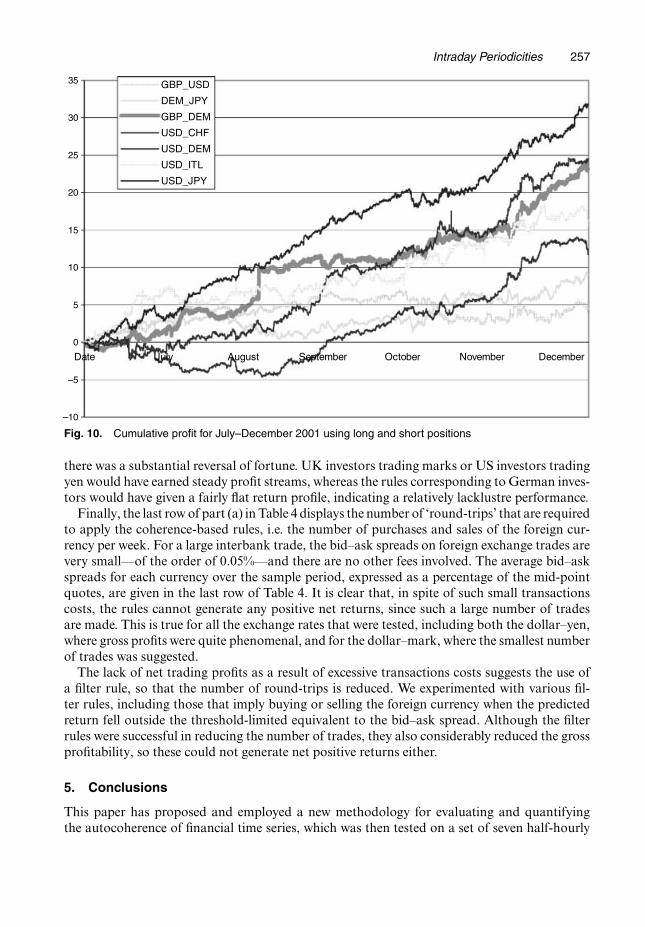
Fig. 10 shows the cumulative returns for the long and short trading rules based on the signalcoherence concept. Buying and selling German marks is the only activity that is seen to lose anAmerican investor money for a protracted period. Trading in German marks using the methodsdescribed above would have been a loss-making activity from July until mid-September when


–10

–5

0

5

10

15

20

25

30

35

Date July August September October November December

GBP_USD

DEM_JPY

GBP_DEM

USD_CHF

USD_DEM

USD_ITL

USD_JPY

Fig. 10. Cumulative profit for July–December 2001 using long and short positions

there was a substantial reversal of fortune. UK investors trading marks or US investors tradingyen would have earned steady profit streams, whereas the rules corresponding to German inves-tors would have given a fairly flat return profile, indicating a relatively lacklustre performance.

Finally, the last row of part (a) in Table 4 displays the number of ‘round-trips’ that are requiredto apply the coherence-based rules, i.e. the number of purchases and sales of the foreign cur-rency per week. For a large interbank trade, the bid–ask spreads on foreign exchange trades arevery small—of the order of 0.05%—and there are no other fees involved. The average bid–askspreads for each currency over the sample period, expressed as a percentage of the mid-pointquotes, are given in the last row of Table 4. It is clear that, in spite of such small transactionscosts, the rules cannot generate any positive net returns, since such a large number of tradesare made. This is true for all the exchange rates that were tested, including both the dollar–yen,where gross profits were quite phenomenal, and for the dollar–mark, where the smallest numberof trades was suggested.

The lack of net trading profits as a result of excessive transactions costs suggests the use ofa filter rule, so that the number of round-trips is reduced. We experimented with various fil-ter rules, including those that imply buying or selling the foreign currency when the predictedreturn fell outside the threshold-limited equivalent to the bid–ask spread. Although the filterrules were successful in reducing the number of trades, they also considerably reduced the grossprofitability, so these could not generate net positive returns either.

5. Conclusions

This paper has proposed and employed a new methodology for evaluating and quantifyingthe autocoherence of financial time series, which was then tested on a set of seven half-hourly


exchange rate returns. Significant coherence for at least one frequency across frames was revealedfor all series. Overall we find the signal coherence to be maximal at the 15-h, 12-h and especially8-h frequencies. In the last case, this may be attributable to the opening and closing of the world’sthree financial market time zones.

The mean frame estimate was cleaned by removing all incoherent frequency components, andthe remaining estimates were used to generate trading rules based on these most stable cyclicalfeatures. The strategies were employed to construct several performance evaluation measuresthat are commonly used by financial market practitioners. These trading rules could generate inmost cases phenomenal gross profits that were statistically significant and showed evidence ofsignificant market timing ability, but the very large number of trades required meant that thesewere more than wiped out by transaction costs.

Our analysis could be extended and enhanced in various ways. First, in the out-of-sampleevaluation, improved trading performance is likely to result from the use of a rolling window ofdata, where a one-frame-ahead forecast is produced and the trading rule implemented, and thenthe sample rolled forward by one frame. Second, the use of a 1% significance level cut-off fordetermining the coherent parts of the signal is somewhat arbitrary, and sensitivity analysis couldbe conducted to determine the effect on profitability of increasing or reducing this threshold. Ifthis threshold is set too high, then important cycles in the data will not be employed, whereas ifit is set too low it is comparable with the effect of including irrelevant regressors in a standardtime series regression model used for forecasting.

A third possibility would be an examination of a much longer run of lower frequency data,so that the frequency of transacting would be reduced and potential returns per trade increasedto mitigate the effect of the bid–ask spread on profitability. These factors suggest that the profit-ability that is demonstrated in this paper is probably an understatement of that which is possibleif the approach is further refined and optimized. In any case, there are many financial agentswho do not require immediacy when making foreign exchange trades. US multinational compa-nies, for example, may desire to reduce their holdings in marks and to increase their holding inpounds, and they may be willing to make the trades at any time in the near future, although theexact time is not of concern to them. Such agents would be forced to incur the transaction costswhenever they trade, and our research suggests that there are better methods for selecting thetime to trade than doing so at random. Some large financial institutions (e.g. hedge funds) maybe able to trade at much lower transaction costs than the figures that we quote, thus significantlyimproving net returns. We conjecture that the methodology that is employed in this paper couldbe a widely applicable tool for market microstructure researchers and statistical arbitrageurs,which will enable them to detect, quantify and rank the various periodic components in financialdata better.

Acknowledgements

The authors are grateful for comments from two referees and from the Joint Editor. The usualdisclaimer applies.

References

Admati, A. R. and Pfleiderer, P. (1988) A theory of intraday patterns: volume and price variability. Rev. Finan.Stud., 1, 3–40.

Andersen, T. G. and Bollerslev, T. (1997a) Intraday periodicity and volatility persistence in financial markets.J. Empir. Finan., 4, 115–158.

Andersen, T. G. and Bollerslev, T. (1997b) Heterogeneous information arrivals and return volatility dynamics:uncovering the long-run in high frequency returns. J. Finan., 52, 975–1005.


Andersen, T. G. and Bollerslev, T. (1998) Deutsche-mark-dollar volatility: intraday activity patterns, macro-economic announcements and longer run dependencies. J. Finan., 53, 219–265.

Baillie, R. T. and Bollerslev, T. (1991) Intra-day and inter-market volatility in foreign exchange rates. Rev. Econ.Stud., 58, 565–585.

Bertoneche, M. L. (1979) Spectral analysis of stock market prices. J. Bankng Finan., 3, 201–208.Brock, W. A., Dechert, W. D. and Scheinkman, J. A. (1987) A test for independence based on the correlation

dimension. Mimeo. Department of Economics, University of Wisconsin, Madison.Chan, K. C., Christie, W. G. and Schultz, P. H. (1995) Market structure and the intraday pattern of bid-ask

spreads for NASDAQ securities. J. Bus., 68, 35–60.Ding, D. K. and Lau, S. T. (2001) An analysis of transactions data for the stock exchange of Singapore: patterns,

absolute price change, trade size and number of transactions. J. Bus. Finan. Accountng, 28, 151–174.Durlauf, S. N. (1991) Spectral based testing of the Martingale hypothesis. J. Econometr., 50, 355–376.Engle, R. F. (1982) Autoregressive conditional heteroscedasticity with estimates of the variance of United King-

dom inflation. Econometrica, 50, 987–1007.Fong, W. M. and Ouliaris, S. (1995) Spectral tests of the Martingale hypothesis for exchange rates. J. Appl.

Econometr., 10, 255–271.French, K. R. (1980) Stock returns and the weekend effect. J. Finan. Econ., 8, 55–69.Gardner, W. A. (1985) Introduction to Random Processes and Application to Signal and Systems. New York:

Macmillan.Gardner, W. A. (ed.) (1994) Cyclostationarity in Communications and Signal Processing. New York: Institution

of Electrical and Electronics Engineers Press.Gardner, W. A. and Franks, L. E. (1975) Characterisation of cyclostationary random signal processes. IEEE

Trans. Inform. Theory, 21, 4–14.Gibbons, M. R. and Hess, P. J. (1981) Day of the week effects and asset returns. J. Bus., 54, 579–596.Gladyshev, E. G. (1961) Periodically correlated random sequences. Sov. Math. Dokl., 2, 385–388.Granger, C. W. J. (1966) The typical spectral shape of an economic variable. Econometrica, 34, 150–161.Granger, C. W. J. and Hatanaka, M. (1964) Spectral Analysis of Economic Time Series. Princeton: Princeton

University Press.Granger, C. W. J. and Morgenstern, O. (1963) Spectral analysis of stock market prices. Kyklos, 16, 1–27.Harris, L. (1986) A transaction data study of weekly and intradaily patterns in stock returns. J. Finan. Econ., 16,

99–118.Henriksson, R. D. and Merton, R. C. (1981) On market timing and investment performance: II, statistical pro-

cedures for evaluating forecasting skills. J. Bus., 54, 513–533.Hilliard, J. E. (1979) The relationship between equity indices on world exchanges. J. Finan., 34, 103–114.Hinich, M. J. (2000) A statistical theory of signal coherence. J. Ocean. Engng, 25, 256–261.Hinich, M. J. (2003) Detecting randomly modulated pulses in noise. Signal Process., 83, 1349–1352.Ito, T. and Roley, V. V. (1987) News for the US and Japan: which moves the yen-dollar exchange rate? J. Monet.

Econ., 19, 255–277.Jaffe, J. R. and Westerfield, R. (1985) The weekend effect in common stock returns: the international evidence.

J. Finan., 40, 432–454.Keim, D. B. and Stambaugh, R. F. (1984) A further investigation of the weekend effect in stock returns. J. Finan.,

39, 819–840.Merton, R. C. (1981) On market timing and investment performance: I, an equilibrium theory of value for market

forecasts. J. Bus., 54, 363–406.Pesaran, M. H. and Timmerman, A. (1992) A simple non-parametric test of predictive performance. J. Bus. Econ.

Statist., 10, 461–465.Pesaran, M. H. and Timmerman, A. (1994) A generalisation of the non-parametric Henriksson-Merton test of

market timing. Econ. Lett., 44, 1–7.Rogalski, R. J. (1984) New findings regarding day of the week returns over trading and non-trading periods: a

note. J. Finan., 39, 1603–1614.Smirlock, M. and Starks, L. (1986) Day-of-the-week effects and intraday effects in stock returns. J. Finan. Econ.,

17, 197–210.Smith, K. L. (1999) Major world equity market interdependence: evidence from cross spectral analysis. J. Bus.

Finan. Accountng, 26, 365–392.Upson, R. B. (1972) Random walk and forward exchange rates: a spectral analysis. J. Finan. Quant. Anal., 7,

1897–1905.Wood, R. A., McUnish, T. H. and Ord, J. K. (1985) An investigation of transactions data for NYSE stocks.

J. Finan., 40, 723–739.Yadav, P. K. and Pope, P. F. (1992) Intraweek and intraday seasonalities on stock market risk premia: cash and

futures. J. Bankng Finan., 16, 233–270.

Detecting intraday periodicities with application to high ... · 2006 Royal Statistical Society...

Documents

Transcript of Detecting intraday periodicities with application to high ... · 2006 Royal Statistical Society...