Describing Within-Person Fluctuation over Time using ... · person (although people can have...

Describing Within-Person Fluctuation over Time using

Alternative Covariance Structures

Lecture 2 1

• Topics: The Big Picture ACS models using the R matrix only Introducing the G, Z, and V matrices ACS models combining the G and R matrices

Modeling Change vs. Fluctuation

Model for the Means:• WP Change describe pattern of average change (over “time”)• WP Fluctuation *may* not need anything (if no systematic change)

Model for the Variances:• WP Change describe individual differences in change (random effects)

this allows variances and covariances to differ over time• WP Fluctuation describe pattern of variances and covariances over time

Lecture 2 2

Time

Pure WP Change

Time

Pure WP FluctuationOur focus right now

Big Picture Framework: Models for the Variance in Longitudinal Data

Lecture 2 3

Pars

imon

y

Goo

d fi

t

Unstructured (UN)Compound Symmetry (CS)

NAME ...THAT … STRUCTURE!

Most useful model: likely somewhere in between!

UnivariateRM ANOVA

Multivariate RM ANOVA

What is the pattern of variance and covariance over time?

CS and UN are just two of the many, many options available within MLM, including random effects models (for change) and alternative covariance structure models (for fluctuation).

2T1 T12 T13 T14

2T21 T2 T23 T24

2T31 T32 T3 T43

2T41 T42 T43 T4

σ σ σ σ

σ σ σ σ

σ σ σ σ

σ σ σ σ

0 0 0 0

0 0 0 0

0 0 0 0

0 0 0 0

2 2 2 2 2U e U U U

2 2 2 2 2U U e U U

2 2 2 2 2U U U e U

2 2 2 2 2U U U U e

Relative Model Fit by Model Side• Nested models (i.e., in which one is a subset of the other)

can now differ from each other in two important ways

• Model for the Means which predictors and which fixed effects of them are included in the model Does not require assessment of relative model fit using LL or −2LL

(can still use univariate or multivariate Wald tests for this)

• Model for the Variance what the pattern of variance and covariance of residuals from the same unit should be DOES require assessment of relative model fit using LL or −2LL Cannot use the Wald test p-values that show up on the output for

testing significance of variances because those p-values are use a two-sided sampling distribution for what the variance could be (but variances cannot be negative, so those p-values are not valid)

Lecture 2 4

Comparing Models for the Variance• ACS models require assessment of relative model fit: how

well does the model fit relative to other possible models?

• Relative fit is indexed by overall model log-likelihood (LL): Log of likelihood for each person’s outcomes given model parameters Sum log-likelihoods across all independent persons = model LL Two flavors: Maximum Likelihood (ML) or Restricted ML (REML)

• What you get for this on your output varies by software…

• Given as −2*log likelihood (−2LL) in SAS or SPSS MIXED:−2LL gives BADNESS of fit, so smaller value = better model

• Given as just log-likelihood (LL) in STATA MIXED and Mplus:LL gives GOODNESS of fit, so bigger value = better model

Lecture 2 5

Comparing Models for the Variance• Two main questions in choosing a model for the variance: How does the variance of the residuals differ across occasions?

How are the residuals from the same unit correlated?

• Nested models are compared using a “likelihood ratio test”: −2∆LL test (aka, “χ2 test” in SEM; “deviance difference test” in MLM)

1. Calculate −2∆LL: if given −2LL, do −2∆LL = (−2LLfewer) – (−2LLmore)if given LL, do −2∆LL = −2 *(LLfewer – LLmore)

2. Calculate ∆df = (# Parmsmore) – (# Parmsfewer)

3. Compare −2∆LL to χ2 distribution with df = ∆df

4. Get p-value from CHIDIST in excel or LRTEST option in STATA

Lecture 2 6

Results of 1. & 2. must be positive values!

“fewer” = from model with fewer parameters“more” = from model with more parameters

Comparing Models for the Variance• What your p-value for the −2∆LL test means: If you ADD parameters, then your model can get better

(if −2∆LL test is significant ) or not better (not significant) If you REMOVE parameters, then your model can get worse

(if −2∆LL test is significant ) or not worse (not significant)

• Nested or non-nested models can also be compared by Information Criteria that also reflect model parsimony No significance tests or critical values, just “smaller is better” AIC = Akaike IC = −2LL + 2 *(#parameters) BIC = Bayesian IC = −2LL + log(N)*(#parameters) What “parameters” means depends on flavor (except in STATA):

ML = ALL parameters; REML = variance model parameters only

Lecture 2 7

Big Picture Framework: Models for the Variance in Longitudinal Data

Lecture 2 8

Pars

imon

y

Goo

d fi

t

Unstructured (UN)Compound Symmetry (CS)

NAME ...THAT … STRUCTURE!

Most useful model: likely somewhere in between!

UnivariateRM ANOVA

Multivariate RM ANOVA

What is the pattern of variance and covariance over time?

CS and UN are just two of the many, many options available within MLM, including random effects models (for change) and alternative covariance structure models (for fluctuation).

2T1 T12 T13 T14

2T21 T2 T23 T24

2T31 T32 T3 T43

2T41 T42 T43 T4

σ σ σ σ

σ σ σ σ

σ σ σ σ

σ σ σ σ

0 0 0 0

0 0 0 0

0 0 0 0

0 0 0 0

2 2 2 2 2U e U U U

2 2 2 2 2U U e U U

2 2 2 2 2U U U e U

2 2 2 2 2U U U U e

Alternative Covariance Structure Models• Useful in predicting patterns of variance and covariance that

arise from fluctuation in the outcome over time: Variances: Same (homogeneous) or different (heterogeneous)? Covariances: Same or different? If different, what is the pattern?

Models with heterogeneous variances predict correlation instead of covariance Often don’t need any fixed effects for systematic effects of time in the

model for the means (although this is always an empirical question)

• Limitations for most of the ACS models: Require equal-interval occasions (they are based on idea of “time lag”) Require balanced time across persons (no intermediate time values) But do not require complete data (unlike when CS and UN are

estimated via least squares in ANOVA instead of ML/REML in MLM)

• ACS models will require some new terminology and tests…

Lecture 2 9

Two Families of ACS Models• So far, we’ve referred to the variance and covariance matrix of the

longitudinal outcomes as the R matrix We now refer to these as “R-only models” (use REPEATED statement only) Although the R matrix is actually specified per individual, ACS models

usually assume the same R matrix for everyone R matrix is symmetric with dimensions n x n, in which n = # occasions per

person (although people can have missing data, the same set of possibleoccasions is required across people to use most R-only models)

• 3 other matrices we’ll see in “G and R combined” ACS models: G = matrix of random effects variances and covariances (stay tuned) Z = matrix of values for predictors that have random effects (stay tuned) V = symmetric n x n matrix of total variance and covariance over time

If the model includes random effects, then G and Z get combined with R to make Vas (accomplished by adding the RANDOM statement)

If the model does NOT include random effects in G, then … so, R-only

Lecture 2 10

Review: Covariances and Correlations

• Given the standard deviation (as Variance) at each occasion, either the correlation and covariance can be calculated given the other

• ACS models with homogeneous variances tend to be specified in terms of variance and covariance Given same variance over time, same covariance same correlation

• ACS models with heterogeneous variance tend to be specified in terms of variance and correlation Different variances over time different covariances over time, even if the

correlation is the same (so only correlation is estimated directly)

Lecture 2 11

y1,y2y1,y2

y1 y2

y1,y2 y1,y2 y1 y2

CovarianceCorrelation

Variance * Variance Covariance Correlation * Variance * Variance



Lecture 2 12


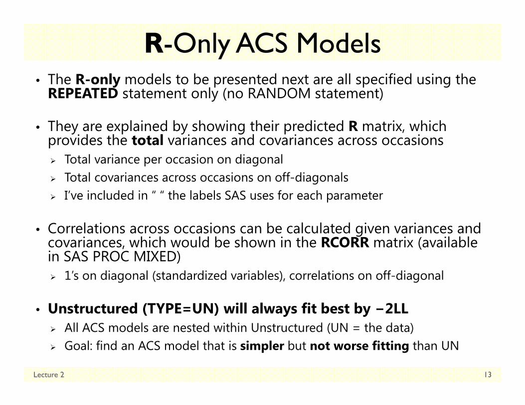
R-Only ACS Models• The R-only models to be presented next are all specified using the

REPEATED statement only (no RANDOM statement)

• They are explained by showing their predicted R matrix, which provides the total variances and covariances across occasions Total variance per occasion on diagonal Total covariances across occasions on off-diagonals I’ve included in “ “ the labels SAS uses for each parameter

• Correlations across occasions can be calculated given variances and covariances, which would be shown in the RCORR matrix (available in SAS PROC MIXED) 1’s on diagonal (standardized variables), correlations on off-diagonal

• Unstructured (TYPE=UN) will always fit best by −2LL All ACS models are nested within Unstructured (UN = the data) Goal: find an ACS model that is simpler but not worse fitting than UN

Lecture 2 13

R-Only ACS Models: CS/CSH• Compound Symmetry: TYPE=CS

2 parameters: 1 “residual” variance 1 “CS” covariance

across occasions Constant total variance: CS σ Constant total covariance: CS

• Compound Symmetry Heterogeneous: TYPE=CSH n+1 parameters:

n separate “Var(n)”total variances

1 “CSH” total correlationacross occasions

Separate total variances are estimated directly Still constant total correlation: CSH (but has non-constant covariances)

Lecture 2 14

2e

2e

2e

2e

CS CS CS CS

CS CS CS CS

CS CS CS CS

CS CS CS CS

2T1 T1 T2 T1 T3 T1 T4

2T2 T1 T2 T2 T3 T2 T4

2T3 T1 T3 T2 T3 T3 T4

2T4 T1 T4 T2 T4 T3 T4

σ CSH CSH CSH

CSH σ CSH CSH

CSH CSH σ CSH

CSH CSH CSH σ

R-Only ACS Models: AR1/ARH1• 1st Order Auto-Regressive: TYPE=AR(1)

2 parameters: 1 constant total variance

(mislabeled “residual”) 1 “AR1” total auto-correlation rT

across occasions r is lag-1 correlation, r is lag-2 correlation, r is lag-3 correlation….

• 1st Order Auto-Regressive Heterogeneous: TYPE=ARH(1) n+1 parameters:


1 “ARH1” total auto-correlation rT across occasions

r is lag-1 correlation, r is lag-2 correlation, r is lag-3 correlation….

Lecture 2 15

2 1 2 2 2 3 2T T T T T T T

1 2 2 1 2 2 2T T T T T T T2 2 1 2 2 1 2T T T T T T T3 2 2 2 1 2 2T T T T T T T

σ r σ r σ r σr σ σ r σ r σr σ r σ σ r σr σ r σ r σ σ

2 1 2 3T1 T T1 T2 T T1 T3 T T1 T4

1 2 1 2T T2 T1 T2 T T2 T3 T T2 T42 1 2 1T T3 T1 T T3 T2 T3 T T3 T43 2 1 2T T4 T1 T T4 T2 T T4 T3 T4

σ r r rr σ r rr r σ rr r r σ

R-Only ACS Models: TOEPn/TOEPHn• Toeplitz(n): TYPE=TOEP(n)

n parameters: 1 constant total variance

(mislabeled “residual”) n−1 “TOEP(lag)” cTn banded

total covariances across occasions c is lag-1 covariance, c is lag-2 covariance, c is lag-3 covariance….

• Toeplitz Heterogeneous(n): TYPE=TOEPH(n) n + (n−1) parameters:


n−1 “TOEPH(lag)” rTnbanded total correlations across occasions

r is lag-1 correlation, r is lag-2 correlation, r is lag-3 correlation….

Lecture 2 16

2T

2T1 T

2T2 T1 T

2T3 T2 T1 T

σc σc c σc c c σ

2T1 T1 T1 T2 T2 T1 T3 T3 T1 T4

2T1 T2 T1 T2 T1 T2 T3 T2 T2 T4

2T2 T3 T1 T1 T3 T2 T3 T1 T3 T4

2T3 T4 T1 T2 T4 T2 T1 T4 T3 T4

σ r r rr σ r rr r σ rr r r σ

Comparing R-only ACS Models• Baseline models: CS =simplest, UN = most complex

Relative to CS, more complex models fit “better” or “not better” Relative to UN, less complex models fit “worse” or “not worse”

• Other rules of nesting and model comparisons: Homogeneous variance models are nested within heterogeneous

variance models (e.g., CS in CSH, AR1 in ARH1, TOEP in TOEPH) CS and AR1 are each nested within TOEP (i.e., TOEP can become

CS or AR1 through restrictions of its covariance patterns) CS and AR1 are not nested (because both have 2 parameters) R-only models differ in unbounded parameters, so can be compared

using regular −2∆LL tests (instead of mixture −2∆LL tests) Good idea to start by assuming heterogeneous variances until you settle

on the covariance pattern, then test if het. var. are still necessary When in doubt, just compare AIC and BIC (useful even with −2∆LL tests)

Lecture 2 17



Lecture 2 18


The Other Family of ACS Models• R-only models directly predict the total variance and covariance• G and R models indirectly predict the total variance and covariance

through between-person (BP) and within-person (WP) sources of variance and covariance So, for this model: yti = β0 + U0i + eti

BP = G matrix of level-2 random effect (U0i) variances and covariances Which effects get to be random (whose variance and covariances are then

included in G) is specified using the RANDOM statement (always TYPE=UN) Our ACS models have a random intercept only, so G is 1x1 scalar of

WP = R matrix of level-1 (eti) residual variances and covariances The n x n R matrix of residual variances and covariances that remain after

controlling for random intercept variance is then modeled with REPEATED Total = V = n x n matrix of total variance and covariance over time that

results from putting G and R together: Z is a matrix that holds the values of predictors with random effects,

but Z will be an n x 1 column of 1’s for now (random intercept only)

Lecture 2 19

A “Random Intercept” (G and R) Model

Lecture 2 20

0

2Uτ

Unstructured G Matrix(RANDOM statement)Each person has same 1 x 1 Gmatrix (no covariance across persons in two-level model)

Diagonal (VC) R Matrix(REPEATED statement)

Each person has same n x n Rmatrix equal variances and 0

covariances across time (no covariance across persons)

Level 2, BP Variance Level 1, WP Variance

Total Predicted Data Matrix is called V Matrix

Random Intercept Variance only

Residual Variance only

0 0 0 0

0 0 0 0

0 0 0 0

0 0 0 0

2 2 2 2 2U e U U U

2 2 2 2 2U U e U U

2 2 2 2 2U U U e U

2 2 2 2 2U U U U e

2e

2e

2e

2e

σ 0 0 0

0 σ 0 0

0 0 σ 0

0 0 0 σ

CS as a “Random Intercept” Model

Lecture 2 21

0 0 0 0

0 0 0 0

0

0 0

T

2 2 2 2 22 U e U U Ue2 2 2 2 22U U e U Ue2

U 2 2e U U

2e

* *

0 0 010 0 01

1 1 1 11 0 0 01 0 0 0

V Z G Z R V

V0 0

0 0 0 0

2 2 2 2U e U

2 2 2 2 2U U U U e

RI and DIAG: Total predicted data matrix is called V matrix, created from the G [TYPE=UN] and R [TYPE=VC] matrices as follows:

2e

2e

2e

2e

CS CS CS CS

CS CS CS CS

CS CS CS CS

CS CS CS CS

Does the end result V look familiar? It should: CS =

So if the R-only CS model (the simplest baseline) can be specified equivalently using G and R, can we do the same for the R-only UN model(the most complex baseline)?

Absolutely! ...with one small catch

Z represents n per person

UN via a “Random Intercept” Model

Lecture 2 22

0

0

T

22 Ue1 e12 e132

e21 e2 e23 e242U 2

e31 e32 e3 e342

e42 e43 e4

* *

σ σ 01σ σ σ1

1 1 1 11 σ σ σ1 0 σ σ

V Z G Z R V

V

0 0 0

0 0 0 0

0 0 0 0

0 0 0 0

2 2 2 2e1 U e12 U e13 U

2 2 2 2 2U e21 U e2 U e23 U e24

2 2 2 2 2U e31 U e32 U e3 U e34

2 2 2 2 2U U e42 U e43 U e4

σ σ

σ σ σ

σ σ σ

σ σ

RI and UNn−1: Total predicted data matrix is called V matrix, created from the G [TYPE=UN] and R [TYPE=UN(n−1)] matrices as follows:

This RI and UNn−1 model is equivalent to (makes same predictions as) the R-only UN model. But it shows the residual (not total) covariances.

Because we can’t estimate all possible variances and covariances in the Rmatrix and also estimate the random intercept variance τ in the G matrix, we have to eliminate the last R matrix covariance by setting it to 0.

Accordingly, in the RI and UNn−1 model, the random intercept variance τ takes on the value of the covariance for the first and last occasions.

Rationale for G and R ACS models• Modeling WP fluctuation traditionally involves using R only (no G) Total BP + WP variance described by just R matrix (so R=V) Correlations would still be expected even at distant time lags because of

constant individual differences (i.e., the BP random intercept)

Resulting R-only model may require lots of estimated parameters as a resulte.g., 8 time points? Pry need a 7-lag Toeplitz(8) model

• Why not take out the primary reason for the covariance across occasions (the random intercept variance) and see what’s left? Random intercept variance in G control for person mean differences

THEN predict just the residual variance/covariance in R, not the total

Resulting model may be more parsimonious (e.g., maybe only lag1 or lag2 occasions are still related after removing as a source of covariance)

Has the advantage of still distinguishing BP from WP variance (useful for descriptive purposes and for calculating effect sizes later)

Lecture 2 23

Random Intercept + Diagonal R Models

Lecture 2 24

RI and DIAG: V is created from G [TYPE=UN] and R [TYPE=VC]:homogeneous residual variances; no residual covariances

RI and DIAGH: V is created from G [TYPE=UN] and R [TYPE=UN(1)]:heterogeneous residual variances; no residual covariances

0 0 0 0

0 0 0 0

0

0 0

T

2 2 2 2 22 U e U U Ue2 2 2 2 22U U e U Ue2

U 2 2e U U

2e

* * 0 0 01

0 0 01 1 1 1 1

1 0 0 01 0 0 0

V Z G Z R V

V0 0

0 0 0 0

2 2 2 2U e U

2 2 2 2 2U U U U e

0 0 0 0

0 0 0

0

T

2 2 2 2 22 U e1 U U Ue12 2 22U U e2 Ue22

U 2e3

2e4

* * 0 0 01

0 0 01 1 1 1 1

1 0 0 01 0 0 0

V Z G Z R V

V 0

0 0 0 0

0 0 0 0

2 2U

2 2 2 2 2U U U e3 U

2 2 2 2 2U U U U e4

Same fit as R-only CS

NOT same fit as R-only CSH

Random Intercept + AR1 R Models

Lecture 2 25

RI and AR1: V is created from G [TYPE=UN] and R [TYPE=AR(1)]:homogeneous residual variances; auto-regressive lagged residual covariances

RI and ARH1: V is created from G [TYPE=UN] and R [TYPE=ARH(1)]:heterogeneous residual variances; auto-regressive lagged residual covariances

0

T

2 1 2 2 2 3 2e e e e e e e

1 2 2 1 2 2 22 e e e e e e eU 2 2 1 2 2 1 2

e e e e e e e3 2e e e

* * σ r σ r σ r σ1

r σ σ r σ r σ1 1 1 1 11 r σ r σ σ r σ1 r σ r

V Z G Z R V

V

0 0 0 0

0 0 0 0

0 0 0 0

0 0 0 0

2 2 2 1 2 2 2 2 2 3 2U e U e e U e e U e e

2 1 2 2 2 2 1 2 2 2 2U e e U e U e e U e e2 2 2 2 1 2 2 2 2 1 2U e e U e e U e U e e

2 2 1 2 2 2 3 2 2 2 2 2 1 2 2 2e e e e U e e U e e U e e U e

r σ r σ r σr σ r σ r σr σ r σ r σ

σ r σ σ r σ r σ r σ

0

T

2 1 2 3e1 e e1 e2 e e1 e3 e e1 e4

12 e e2U

* * σ r σ σ r σ σ r σ σ1

r σ σ1 1 1 1 111

V Z G Z R V

V

0 0 0 0

0 0 0 0

2 2 2 1 2 2 2 3U e1 U e e1 e2 U e e1 e3 U e e1 e4

2 1 2 2 2 1 2 22 1 2U e e2 e1 U e2 U e e2 e3 U e e2 ee1 e2 e e2 e3 e e2 e4

2 1 2 1e e3 e1 e e3 e2 e3 e e3 e43 2 1 2e e4 e1 e e4 e2 e e4 e3 e4

r σ σ r σ σ r σ σr σ σ r σ σ r σ σσ r σ σ r σ σ

r σ σ r σ σ σ r σ σr σ σ r σ σ r σ σ σ

0 0 0 0

0 0 0 0

42 2 2 1 2 2 2 1U e e3 e1 U e e3 e2 U e3 U e e3 e42 3 2 2 2 1 2 2U e e4 e1 U e e4 e2 U e e4 e3 U e4

r σ σ r σ σ r σ σr σ σ r σ σ r σ σ

Random Intercept + TOEPn−1 R Models

Lecture 2 26

RI and TOEPn−1: V is created from G [TYPE=UN] and R [TYPE=TOEP(n−1)]: homogeneous residual variances; banded residual covariances

RI and TOEPHn−1: V is created from G [TYPE=UN] and R [TYPE=TOEPH(n−1)]: homogeneous residual variances; banded residual covariances

0 0 0 0

0

0

T

2 2 2 2 22 U e U e1 U e2 Ue e1 e22

Ue1 e e1 e22U 2

e2 e1 e e12

e2 e1 e

* * c cσ c c 01

c σ c c11 1 1 1

1 c c σ c1 0 c c σ

V Z G Z R V

V 0 0 0

0 0 0 0

0 0 0 0

2 2 2 2 2e1 U e U e1 U e2

2 2 2 2 2U e2 U e1 U e U e1

2 2 2 2 2U U e2 U e1 U e

c c c

c c c

c c

0

T

2e1 e1 e1 e2 e2 e1 e3

2e1 e2 e1 e2 e1 e2

U

* * σ r σ σ r σ σ 01

r σ σ σ r σ11 1 1 1

11

V Z G Z R V

V

0 0 0 0

0 0 0 0

0 0

2 2 2 2 2U e1 U e1 e1 e2 U e2 e1 e3 U

2 2 2 2 2U e1 e2 e1 U e2 U e1 e2 e3 U e2 e2 e42 e3 e2 e2 e4

2 2 2e2 e3 e1 e1 e3 e2 e3 e1 e3 e4 U e2 e3 e1 U e1 e3

2e2 e4 e2 e1 e4 e3 e4

r σ σ r σ σ

r σ σ r σ σ r σ σσ r σ σ

r σ σ r σ σ σ r σ σ r σ σ r σ σ

0 r σ σ r σ σ σ

0 0

0 0 0 0

2 2 2e2 U e3 U e1 e3 e4

2 2 2 2 2U U e2 e4 e2 U e1 e4 e3 U e4

r σ σ

r σ σ r σ σ

Same fit as R-only TOEP(n)

Because of τ , highest lag

covariance in Rmust be set to 0 for model to be identified

NOT same fit as R-only TOEPH(n)

Random Intercept + TOEP2 R Models

Lecture 2 27

RI and TOEP2: V is created from G [TYPE=UN] and R [TYPE=TOEP(2)]: homogeneous residual variances; banded residual covariance at lag1 only

RI and TOEPH1: V is created from G [TYPE=UN] and R [TYPE=TOEPH(2)]: homogeneous residual variances; banded residual covariance at lag1 only

0 0 0 0

0 0

0

T

2 2 2 2 22 U e U e1 U Ue e12 22U e1 U ee1 e e12

U 2e1 e e1

2e1 e

* * cσ c 0 01

cc σ c 011 1 1 1

1 0 c σ c1 0 0 c σ

V Z G Z R V

V 0 0

0 0 0 0

0 0 0 0

2 2 2U e1 U

2 2 2 2 2U U e1 U e U e1

2 2 2 2 2U U U e1 U e

c

c c

c

0

T

2e1 e1 e1 e2

2e1 e2 e1 e2 e1 e2 e32

Ue

* * σ r σ σ 0 01

r σ σ σ r σ σ 011 1 1 1

1 0 r1

V Z G Z R V

V

0 0 0 0

0 0 0 0

0 0 0 0

0 0 0 0

2 2 2 2 2U e1 U e1 e1 e2 U U

2 2 2 2 2U e1 e2 e1 U e2 U e1 e2 e3 U

2 2 2 2 2 21 e3 e2 e3 e1 e3 e4 U U e1 e3 e2 U e3 U e1 e3 e4

2 2 2 2 2 2e1 e4 e3 e4 U U U e1 e4 e3 U e4

r σ σ

r σ σ r σ σ

σ σ σ r σ σ r σ σ r σ σ

0 0 r σ σ σ r σ σ

Now we can test the need for residual

covariances at higher lags

Map of R-only and G and RACS Models

Lecture 2 28

Homogeneous Variance over Time Heterogeneous (Het.) Variance over Time

R-only Compound Symmetry Het.

R-only Compound Symmetry

Random Intercept & Diagonal R

Num

ber o

f Par

amet

ers i

n H

omog

eneo

us V

aria

nce

Mod

els

Num

ber o

f Par

amet

ers i

n H

eter

ogen

eous

Var

ianc

e M

odel

s

Random Intercept & Diagonal Het. R

R-only First-Order Auto-Regressive

Het.

R-only First-Order

Auto-Regressive Random Intercept & First-Order

Auto-Regressive R

Random Intercept & First-Order Auto-Regressive Het. R

2

2

3

n+1

n+1

n+2

R-only n-1 Lag Toeplitz

Random Intercept & n-2 Lag Toeplitz R

n

3

= ≠

=

Random Intercept & 2-Lag Toeplitz R

Random Intercept & 1-Lag Toeplitz R

4

R-only n-1 Lag Toeplitz Het.

Random Intercept & n-2 Lag Toeplitz Het. R

≠

Random Intercept & 2-Lag Toeplitz Het. R

Random Intercept & 1-Lag Toeplitz Het. R

n+n-1

n+2

n+3

R-only n-order Unstructured

Random Intercept & n-1 order Unstructured R

= n*(n+1) / 2

R-Only Models G and R Combined Models R-Only Models G and R Combined Models

Arrows indicate nesting (end is more complex model)

Stuff to Watch Out For…• If using a random intercept, don’t forget to drop 1 parameter in:

n-1 order UN R: Can’t get all possible elements in R, plus τ in G TOEPn−1: Have to eliminate last lag covariance

• If using a random intercept… Can’t do RI + CS R: Can’t get a constant in R, and then another constant in G Can often test if random intercept helps (e.g., AR1 is nested within RI + AR1)

• If “time” is treated as continuous in the fixed effects, you will need another variable for time that is categorical to use in the syntax: “Continuous Time” on MODEL statement “Categorical Time” on CLASS and REPEATED statements

• Most alternative covariance structure models assume time is balanced across persons with equal intervals across occasions If not, holding correlations of same lag equal doesn’t make sense Other structures can be used for unbalanced time

SP(POW)(time) = AR1 for unbalanced time (see SAS REPEATED statement for others)

Lecture 2 29

Summary: Two Families of ACS Models• R-only models:

Specify R model on REPEATED statement without any random effects variances in G (so no RANDOM statement is used)

Include UN, CS, CSH, AR1, AR1H, TOEPn, TOEPHn (among others)

Total variance and total covariance kept in R, so R = V

Other than CS, does not partition total variance into BP vs. WP

• G and R combined models (so G and R V): Specify random intercept variance τ in G using RANDOM statement,

then specify R model using REPEATED statement

G matrix = Level-2 BP variance and covariance due to U , so R = Level-1 WP variance and covariance of the eti residuals

R models what’s left after accounting for mean differences between persons (via the random intercept variance τ in G)

Lecture 2 30

Syntax for Models for the Variance• Does your model include random intercept variance (for U0i) ?

Use the RANDOM statement G matrix

Random intercept models BP interindividual differences in mean Y

• What about residual variance (for eti) ? Use the REPEATED statement R matrix

WITHOUT a RANDOM statement: R is BP and WP variance together = Total variances and covariances (to model all variation, so R = V)

WITH a RANDOM statement: R is WP variance only = Residual variances and covariances to model WP intraindividual variation G and R put back together = V matrix of total variances and covariances

• The REPEATED statement is always there implicitly… Any model always has at least one residual variance in R matrix

• But the RANDOM statement is only there if you write it G matrix isn’t always necessary (don’t always need random intercept)

Lecture 2 31

Wrapping Up: ACS Models• Even if you just expect fluctuation over time rather than

change, you still should be concerned about accurately predicting the variances and covariances across occasions

• Baseline models (from ANOVA least squares) are CS & UN: Compound Symmetry: Equal variance and covariance over time

Unstructured: All variances & covariances estimated separately

CS and UN via ML or REML estimation allows missing data

• MLM gives us choices in the middle Goal: Get as close to UN as parsimoniously as possible

R-only: Structure TOTAL variation in one matrix (R only)

G+R: Put constant covariance due to random intercept in G, then structural RESIDUAL covariance in R (so that G and R V TOTAL)

Lecture 2 32

Describing Within-Person Fluctuation over Time using ... · person (although people can have...

Documents

Transcript of Describing Within-Person Fluctuation over Time using ... · person (although people can have...