Degradation modeling applied to residual lifetime …nserban/publications/degradmo… · ·...

The Annals of Applied Statistics2011, Vol. 5, No. 2B, 1586–1610DOI: 10.1214/10-AOAS448© Institute of Mathematical Statistics, 2011

DEGRADATION MODELING APPLIED TO RESIDUAL LIFETIMEPREDICTION USING FUNCTIONAL DATA ANALYSIS

BY RENSHENG R. ZHOU1, NICOLETA SERBAN AND NAGI GEBRAEEL1

Georgia Institute of Technology

Sensor-based degradation signals measure the accumulation of damageof an engineering system using sensor technology. Degradation signals canbe used to estimate, for example, the distribution of the remaining life of par-tially degraded systems and/or their components. In this paper we presenta nonparametric degradation modeling framework for making inference onthe evolution of degradation signals that are observed sparsely or over shortintervals of times. Furthermore, an empirical Bayes approach is used to up-date the stochastic parameters of the degradation model in real-time usingtraining degradation signals for online monitoring of components operatingin the field. The primary application of this Bayesian framework is updatingthe residual lifetime up to a degradation threshold of partially degraded com-ponents. We validate our degradation modeling approach using a real-worldcrack growth data set as well as a case study of simulated degradation signals.

1. Introduction. Most failures of engineering systems result from a gradualand irreversible accumulation of damage that occurs during a system’s life cycle.This process is known as degradation [Bogdanoff and Kozin (1985)]. In many ap-plications, it can be very difficult to assess and observe physical degradation, espe-cially when real-time observations are required. However, degradation processesare almost always associated with some manifestations that are much easier toobserve and monitor overtime. Generally, the evolution of these manifestationscan be monitored using sensor technology through a process known as ConditionMonitoring (CM). The observed condition-based signals are known as degradationsignals [Nelson (1990)] and are usually correlated with the underlying physicaldegradation process. Some examples of degradation signals include vibration sig-nals for monitoring excessive wear in rotating machinery, acoustic emissions formonitoring crack propagation, temperature changes and oil debris for monitoringengine lubrication and many others.

Degradation modeling attempts to characterize the evolution of degradation sig-nals. There is a significant number of research works that have focused on degra-dation models; these include models presented in Lu and Meeker (1993), Padgettand Tomlinson (2004), Gebraeel et al. (2005), Müller and Zhang (2005), Gebraeel

Received May 2010; revised October 2010.1Supported in part by the NSF Grant CMMI-0738647.Key words and phrases. Condition Monitoring, functional principal component analysis, non-

parametric estimation, residual life distribution, sparse degradation signal.

1586

http://www.imstat.org/aoas/

http://dx.doi.org/10.1214/10-AOAS448

http://www.imstat.org

DEGRADATION MODELING USING FUNCTIONAL DATA ANALYSIS 1587

FIG. 1. Examples of incomplete degradation signals.

(2006) and Park and Padgett (2006). Many of these models rely on a representa-tive sample of complete degradation signals. A complete degradation signal is acontinuously observed signal that captures the degradation process of a componentfrom a brand “New State” to a completely “Failed State.”

Unfortunately, building a database of complete degradation signals can be veryexpensive and time consuming in applications, such as monitoring of jet engines,turbines, power generating units, structures and bridges and many others. For ex-ample, in applications consisting of relatively static structures such as bridges,degradation usually takes place very slowly (several tens of years). Since the sys-tem is relatively static, it suffices to observe the degradation process at intermittentdiscrete time points. The result is a sparsely observed degradation signal such asthe signals depicted in Figure 1(a). In contrast, in applications consisting of dy-namic systems, such as turbines, generators and machines, degradation cannot bereasonably assessed by sparse measurements. At the same time, continuous ob-servations of the complete degradation process of such systems are economicallyunjustifiable. Usually, the only way to gain a relatively accurate understanding ofthe health/performance of a dynamic system is to monitor its performance over atime interval. In naval maritime applications, power generating units of an aircraftare removed, tested for a short period of time (during which degradation data canbe acquired) and put back into operation. The result is a collection of fragmenteddegradation signals as depicted in Figure 1(b).

In this paper we develop a degradation model that applies to incomplete degra-dation signals as well as complete degradation signals. An incomplete degradationsignal is defined as a signal that consists of sparse observations of the degradationprocess or continuous observations made over short time intervals (fragments).One challenge in such applications is that the evolution of the degradation signalscannot be readily assessed to determine the parametric form of the underlyingdegradation model. This is because one cannot clearly trace how a degradation

1588 R. R. ZHOU, N. SERBAN AND N. GEBRAEEL

signal progresses over time from incomplete observations. For example, is there awell defined parametric model that describes the signals in Figure 1?

To overcome this challenge, the underlying degradation model in this paper isassumed nonparametric. Most degradation models used to characterize the evo-lution of sensor-based degradation signals are parametric models. A commonapproach is to model the degradation signals using a parametric (linear) modelwith random coefficients [Lu and Meeker (1993); Gebraeel et al. (2005); Gebraeel(2006)]. Other modeling approaches assume that the degradation signal follows aBrownian motion process [Doksum and Hoyland (1992); Pettit and Young (1999)]or a Gaussian process with known covariance structure [Padgett and Tomlinson(2004); Park and Padgett (2006)]. In contrast, we assume that the mean and co-variance functions of the degradation process are unknown and they are estimatedbased on an assembly of training incomplete degradation signals. The mean func-tion is estimated using standard nonparametric regression methods such as localsmoothing [Fan and Yao (2003)]. The covariance function is decomposed using theKarhunen–Loève decomposition [Karhunen (1947); Loève (1945)] and estimatedusing the Functional Principal Component Analysis (FPCA) method introducedby Yao, Müller and Wang (2005).

Under the nonparametric modeling framework, one condition for accurate es-timation of the mean and covariance functions is that the degradation processis densely observed throughout its support. However, in applications where thedegradation signals are incompletely sampled, not all degradation signals are ob-served up to the point of failure; in addition, only a few components will survive upto the maximum time point of the degradation process support. Consequently, thedegradation process is commonly under-sampled close to the upper bound of itssupport. To overcome this difficulty, we introduce a nonuniform sampling proce-dure for collecting incomplete degradation signals, which ensures relatively densecoverage throughout the sampling time domain.

One important application of degradation modeling is predicting the lifetime ofcomponents operating in the field. For real-time monitoring, an empirical Bayesapproach is introduced to update the stochastic parameters of the degradationmodel. In this paper we focus on estimation of the distribution of the residuallife up to a degradation threshold for partially degraded components using trainingdegradation signals which are sparsely or completely observed. Other applicationsof the degradation modeling and the Bayesian updating procedure are estimationof the lifetime at a specified degradation level and estimation of the degradationlevel at a specified lifetime.

We evaluate the performance of our methodology using both a crack growthdata set and simulated degradation signals. In these empirical studies we compareparametric to nonparametric degradation modeling, assess the estimation accuracyof the remaining lifetime for complete and incomplete signals, and contrast uni-form vs. nonuniform sampling procedures for acquiring ensembles of incomplete


degradation signals. In both studies there is not a significant decrease in the accu-racy of the residual life estimation when using ensembles of incomplete instead ofcomplete signals. We also highlight the robustness of our approach by comparingit with misspecified parametric models, which are common when the underlyingdegradation process is complicated and sparsely observed. Last, we show in thesimulation study that using a nonuniform sampling procedure that ensures denseobservation of the sampling time domain reduces the estimation error. Based onthese empirical studies, we conclude that the nonparametric approach introducedin this paper is efficient in characterizing the underlying degradation process andit is more robust to model misspecification than parametric approaches, which isparticularly important when the training signals are incompletely observed (sparseor fragmented).

The remainder of the paper is organized as follows. Section 2 discusses the de-velopment of our degradation modeling framework. The empirical Bayes approachfor updating the degradation distribution of a partially degraded component is in-troduced in Section 3. The derivation of the remaining lifetime distribution underthe empirical Bayes approach is presented in Section 4. In Section 5 we introducean experimental design for sampling incomplete degradation signals. We discussperformance results of our methodology using real-world and simulated degrada-tion signals in Section 6 and 7, respectively.

2. Sensor-based degradation modeling. We denote the observed degrada-tion signals Si(tij ), for j = 1, . . . ,mi (mi is the number of observation time pointsfor signal i) and i = 1, . . . , n (n is the number of signals) where {tij }j=1,...,mi

arethe observation time points in a bounded time domain [0,M] for signal i. Notethat M will always be finite since any industrial application has a finite time offailure. We model the distribution of the signals Si(t) by borrowing informationacross multiple degradation signals. We decompose the degradation signal as

Si(t) = μ(t) + Xi(t) + σεi(t),(2.1)

where μ(t) is the underlying trend of the degradation process and is assumed to befixed but unknown, and Xi(t) represents the random deviation from the underlyingdegradation trend. We also assume Xi(t) and εi(t) are independent.

The model in (2.1) is a general decomposition for functional data with variousmodeling alternatives and assumptions for the model components: μ(t), Xi(t),and εi(t). In this paper we discuss one such modeling alternative which applies tosparse and fragmented signals as well as to complete signals and it applies underthe assumption that the observation time points {tij }j=1,...,mi

are fixed but not nec-essarily equally spaced and the assumption that the error terms εi(t) are indepen-dent and identically distributed. Deviations from these assumptions may requiresome modifications to the modeling approach discussed in this paper.

In our modeling approach, the degradation signal Si(t) follows a stochasticprocess with mean μ(t) and stochastic deviations Xi(t) with mean zero and co-variance cov(t, t ′). The mean function μ(t) and the covariance surface cov(t, t ′)


are both assumed to be nonparametric, that is, no prespecified assumption on theirshape. This generalized assumption encompasses the particular cases developedearlier by Gebraeel et al. (2005) and Gebraeel (2006), which assume a linear trend,μ(t) = α + βt where α ∼ N(0, δα) and β ∼ N(0, δβ), and parametric covariancestructure cov(t, t ′) = δα + δβtt ′.

The following steps discuss how we estimate the mean function and the covari-ance surface of our degradation model.

Step 1: We use nonparametric methods to estimate the mean μ(t). In this paperwe use local quadratic smoothing [Fan and Yao (2003)] to allow estimation of themean function under general settings including complete and incomplete (sparseand fragmented) signals. The bandwidth parameter, which controls the smoothinglevel, is selected using the leave-one-curve-out cross-validation method [Rice andSilverman (1991)]. Alternative estimation methods include decomposition of themean function using a basis of functions (e.g., splines, Fourier, wavelets) and es-timate the coefficients using parametric methods. These alternative methods willapply under various signal behaviors (e.g., smooth vs. with sharp changes, uni-formly vs. nonuniformly sampled).

Step 2: The covariance surface is estimated using the demeaned data, Si(t) −μ(t), where μ(t) is the local quadratic smoothing estimate of μ(t). Using theKarhunen–Loéve decomposition [Karhunen (1947); Loève (1945)], the covari-ance, cov(t, t ′) = Cov(Si(t), Si(t

′)), can be expressed as follows:

cov(t, t ′) =∞∑

k=1

λkφk(t)φk(t′), t, t ′ ∈ [0,M],(2.2)

where φk(t) for k = 1,2, . . . are the associated eigenfunctions with support [0,M]and λ1 ≥ λ2 ≥ · · · are the ordered eigenvalues. Based on this decomposition, thedeviations from the underlying degradation trend Xi(t) are decomposed using thefollowing expression:

Xi(tij ) =∞∑

k=1

ξikφk(tij ),(2.3)

where ξik called scores are uncorrelated random effects with mean zero and vari-ance E(ξ2

ik) = λk . The decomposition in equation (2.3) is an infinite sum. Gener-ally, only a small number of eigenvalues are commonly significantly nonzero. Forthe eigenvalues which are approximately zero, the corresponding scores will alsobe approximately zero. Consequently, we use a truncated version of this decompo-sition. Therefore, expression (2.3) can be approximated as follows:

Xi(tij ) =K∑

k=1

ξikφk(tij ),(2.4)

where K is the number of significantly nonzero eigenvalues. We select K to mini-mize the modified Akaike criterion defined by Yao, Müller and Wang (2005).


In the statistical literature this method has been coined Functional PrincipalComponent Analysis (FPCA). The key reference for FPCA is Ramsay and Silver-man [(1997), Chapter 8]. Another important reference is Yao, Müller and Wang(2005), in which the authors derived theoretical results for model parameter con-sistency and asymptotic (n large) distribution results under the assumption that thescores follow a normal distribution.

An alternative method for estimating the covariance function of the processXi(t) is decomposing the covariance function as in equation (2.2) where the basisof functions {φk, k = 1,2, . . .} is fixed [James, Hastie and Sugar (2000)]. However,this approach doesn’t allow dimensionality reduction in the same way FPCA doesand it is not theoretically founded.

3. Degradation model updating. Next, we consider a component operatingin the field called fielded component. Assume that we have observed its degrada-tion signal at a vector of time t = (t1, . . . , tm∗); therefore, S(t) denotes the observedsignal of the testing component, m∗ represents the number of observations andt∗ = tm∗ denotes the latest observation time. In this section we introduce an Em-pirical Bayes approach which allows real-time updating of the distribution of thedegradation process for partially degraded components given the observed signalS(t) and the prior distribution of the scores ξik for k = 1,2, . . . . The prior distri-bution of the scores is estimated empirically from a set of historical degradationsignals.

Proposition 1 illustrates the updating procedure assuming that the prior distribu-tion of the scores is normal and assuming that the mean function μ(t) and the basisof functions φk(t), k = 1, . . . ,K , are fixed. The proof of this proposition followsfrom the theory of Bayesian linear models.

PROPOSITION 1. Assume that S(t) follows

S(t) = μ(t) +K∑

k=1

ξkφk(t) + ε(t),

where the prior distribution of ξk is N(0, λk) with ξ1, . . . , ξK uncorrelated; ε(t)

are independent of ξk for k = 1, . . . ,K ; the distribution of ε(t) is N(0, σ 2) withσ 2 fixed. It follows that the posterior distribution of the scores is

(ξ∗1 , . . . , ξ∗

K)′ ∼ N(Cd,C),

where

C =(

1

σ 2 P(t)′P(t) + −1)−1

and d = 1

σ 2 P(t)′(S(t) − μ(t)

)


with

S(t) = (S(t1), . . . , S(tm∗))′, μ(t) = (μ(t1), . . . ,μ(tm∗))′,(3.1)

= diag(λ1, . . . , λK), P (t) =⎛⎝ φ1(t1) . . . φK(t1)

. . . . . . . . .

φ1(tm∗) . . . φK(tm∗)

⎞⎠ .

In Proposition 1 the prior distribution of the scores is specified by the varianceparameters λk , k = 1, . . . ,K , which are estimated using the degradation modelin Section 2 and based on a set of incomplete or complete training degradationsignals. Specifically, we first apply Functional Principal Component Analysis onthe historical degradation signals which will further provide estimates for the vari-ance parameters λk , k = 1, . . . ,K , and the eigenfunctions φk , k = 1, . . . ,K . Basedon these estimates, we obtain the posterior distributions of the updated scoresξ∗

1 , . . . , ξ∗K since the matrix C and the vector d are fully determined by the eigen-

values λk , k = 1, . . . ,K , and the eigenfunctions φk , k = 1, . . . ,K . The expectationof the posterior scores is nonzero and, therefore, we denote the posterior meanfunction μ∗(t) = μ(t) + ∑K

k=1 E(ξ∗k )φk(t).

Following Proposition 1, the expectation of the posterior distribution followsthe same formula as the conditional expectation estimator in Yao, Müller andWang (2005), equation (4). Generally, this similarity applies under the empiricalBayesian prior derived from FPCA. On the other hand, the sampling distributionof the conditional expectation estimator in Yao, Müller and Wang (2005) is dif-ferent from the posterior distribution of ξ∗

k , k = 1, . . . ,K , since their variances arenot equal. Moreover, the conditional expectation estimator and its mean estimationerror in Yao, Müller and Wang (2005) are conditional on the training observations,whereas the posterior distribution in Proposition 1 is conditional on the observa-tions of a new component.

The advantage of this Bayesian framework is that it unifies the conditional ex-pectation estimation and prediction into a procedure which allows updating thedistribution of the degradation process for a new component. We can therefore usethe posterior distribution of the scores for a partially degraded signal to estimatethe distribution of various statistical summaries, including the lifetime at a speci-fied degradation level and estimation of the degradation level at a specified time.In the next section we discuss one specific application to this updating framework:residual life estimation.

4. Remaining life distribution. In this paper we focus our attention on en-gineering applications where a soft-failure of a system occurs once its underlyingdegradation process reaches a predetermined critical threshold. This critical thresh-old is commonly used to initiate maintenance activities such as repair and/or com-ponent replacement well in advance of catastrophic failure. Consequently, degra-dation data can still be observed beyond the critical threshold. In this section we


describe how our degradation modeling framework is applied to estimate the dis-tribution of remaining life up to a degradation threshold of partially degraded sys-tems.

In the remainder of this section, S∗(·) will denote the underlying degradationprocess of a partially degraded system. Based on the degradation process S∗(·),the failure time of a system is defined as

T = inft∈[0,M]{S

∗(t) ≥ D}.(4.1)

One has to bear in mind that T may not exist if the threshold D is set too high,that is, the component may fail before its degradation signal reaches the threshold.The selection of the failure threshold D is an important problem, however, thisaspect is beyond the scope of this paper. In this work, we assume that T exists,and the threshold D is known a priori. This is a reasonable assumption because inmany industrial applications failure/alarm thresholds are usually based on subjec-tive engineering judgement or well-accepted standards, such as the InternationalStandards Organization (ISO) (e.g., the ISO 2372 is used for defining acceptablevibration threshold levels for different machine classifications). A second assump-tion is that the failure time T is smaller than a maximum failure time M . Thisassumption is also reasonable, as in practice a component may be replaced after agiven period of time even if it did not fail.

The distribution of the residual life (RLD) of a partially degraded component ata fixed time t∗ ∈ [0,M] is estimated assuming that the degradation process S∗(·) ofthe component follows a posterior distribution based on Proposition 1. We estimatethe distribution of the residual life (RLD) using

R(y|t∗) = P(T − t∗ ≤ y|S∗(t) ∼ Gaussian(μ∗(t),Cov∗(t, t ′)), t∗ ≤ T ≤ M

),

where μ∗(t) and Cov∗(t, t ′) are the posterior mean and covariance functions of thedegradation process S∗(·). The derivations of μ∗(t) and Cov∗(t, t ′) are based onthe results of Proposition 1. We note here that the distribution of the RLD aboveis not conditional on the observed signal of the partially degraded component buton the posterior distribution of its degradation process; since the degradation isonly partially observed and most often sparsely sampled, conditioning on the pos-terior distribution will generally provide a more accurate RLD estimator since weincorporate the additional information in the training degradation signals.

Furthermore, we estimate RLD under two assumptions:

A.1 The new component has not failed up to the last observation time point t∗,that is, the failure time becomes

T = inft∈[0,M]{S

∗(t) ≥ D} = inft∈[t∗,M]{S

∗(t) ≥ D} := T ∗.

A.2 We assume the probability that the degradation process S∗(t) crosses back thethreshold D after the failure time T ∗ is negligible, that is, P(S∗(T ∗ + y) <


D) ≈ 0 for all y > 0. This implies, if we condition on y ≥ T ∗ − t∗ > 0, whichis the same as conditioning on T ∗ ≤ t∗+y, P(S∗(t∗+y) < D|T ∗ ≤ t∗+y) ≈0. This further implies

P(S∗(t∗ + y) ≥ D

) = P(S∗(t∗ + y) ≥ D|T ∗ ≤ t∗ + y

)P(T ∗ ≤ t∗ + y)

≈ P(T ∗ ≤ t∗ + y).

Under these two assumptions, the RLD becomes

R(y|t∗) = (by A.1) P(T ∗ − t∗ ≤ y|S∗(t)

) ≈ (by A.2) P(S∗(t∗ + y) ≥ D|S∗(t)

).

The approximation in assumption A.2 is similar to the approximation in the paperby Lu and Meeker (1993) which assumes that the probability of a negative randomslope in the linear model is negligible. One particular case for the assumption A.2to hold is that the signal is monotone. However, monotonicity is not a necessarycondition. Assumption A.2 also holds for nonmonotone signals—an example ofsuch a signal is in Figure 2.

Proposition 2 below describes the updating procedure for RLD of a new com-ponent given the posterior distribution of its degradation process S∗(·) updated upto time t∗. The proof follows directly as a consequence of Proposition 1.

PROPOSITION 2. For a new partially degraded component with its degrada-tion process S∗(·) updated up to time t∗, the residual life distribution is given as

FIG. 2. Example of a signal for which assumption A.2 holds.


follows:

P(T − t∗ ≤ y|S∗(·), T ≥ t∗

) = �Z(g∗(y|t∗)) − �Z(g∗(0|t∗))1 − �Z(g∗(0|t∗)) ,(4.2)

where �Z represents the standard normal cumulative distribution function andg∗(y|t∗) = μ∗(t∗+y)−D√

V ∗(t∗+y)with

μ∗(t∗ + y) = μ(t∗ + y) + (Cd)′p(t∗ + y),

V ∗(t∗ + y) =K∑

k1=1

K∑k2=1

[Ck1,k2φk1(t∗ + y)φk2(t

∗ + y)].

In the above equations, p(t∗ + y) = (φ1(t∗ + y), . . . , φK(t∗ + y))′, and Ck1,k2

refers to the (k1, k2) element of the matrix C.One advantage of obtaining the distribution rather than simply a point estimate

is that we can also derive a confidence interval for the remaining lifetime up to adegradation threshold D. Following the derivation in Proposition 2, a 1 − α confi-dence interval for RLD is [L,U ] such that

P(L ≤ T − t∗ ≤ U |S∗(·), T ≥ t∗

) = 1 − α.

Since we have one equation with two unknowns, the lower—L and the upper—U tails are commonly equally weighted, and, therefore,

�Z(g∗(U |t∗)) − �Z(g∗(0|t∗))1 − �Z(g∗(0|t∗)) = 1 − α

2

and�Z(g∗(L|t∗)) − �Z(g∗(0|t∗))

1 − �Z(g∗(0|t∗)) = α

2.

However, we cannot obtain exact solutions for L and U because we do not have aclosed-form expression for the inverse of the cumulative density function of T − t∗.For example, the first relationship is equivalent to finding U from g∗(U |t∗) = zα1

where zα1 is the 1−α1 quantile of the normal distribution. Using this equation, wewould like to obtain U such that

μ∗(t∗ + U) − D√V ∗(t∗ + U)

= zα1,

which is a nonlinear function of U and its solution does not have a close formexpression. We therefore resort to parametric bootstrap [Efron and Tibshirani(1993); Davison and Hinkley (1997)] to sample from the distribution of T − t∗which will give us a set of realizations from this distribution—T1, T2, . . . , TB . Us-ing these realizations from the distribution of T − t∗, we estimate a quantile boot-strap confidence interval.

The confidence interval estimation procedure is as follows. For b = 1, . . . ,B:


1. Sample ξb = (ξb1 , . . . , ξb

K) from the multivariate normal distribution of the pos-terior scores provided in Proposition 1.

2. Obtain a simulated signal

Sb(t) = μ(t) +K∑

k=1

ξbk φk(t),

where ξbk , k = 1, . . . ,K , are the scores sampled at Step 1.

3. Take Tb = inft∈[0,M]{Sb(t) ≥ D}.Using the sampled values T1, T2, . . . , TB , we compute the empirical α/2 and(1 − α/2) quantiles, Tα/2 and T1−α/2, respectively. We estimate the upper andlower bound of the confidence interval by L = Tα/2 and U = T1−α/2. It followsthat [L, U ] is an approximate 1 − α quantile bootstrap confidence interval for theresidual life time of the fielded component.

An additional approach to the (parametric) bootstrap method described aboveis to (re)sample the signal data resulting in multiple bootstrap samples. For eachbootstrap sample, estimate the residual lifetime using the approach discussed inthis paper; therefore, we obtain a set of realization from the distribution of T − t∗.In contrast to the bootstrap method described above, this alternative bootstrap ap-proach requires estimating the FPCA model for each bootstrap sample which iscomputationally expensive.

5. Sampling scheme. The nonparametric degradation modeling frameworkintroduced in this paper applies to both complete as well as incomplete degradationsignals. For applications involving incomplete degradation signals, it is importantto develop a sampling plan that ensures accurate estimation of the mean functionand the covariance surface. Yao, Müller and Wang (2005) provide theoretical re-sults on the estimation of the covariance surface using FPCA under large n butsmall mi for i = 1, . . . , n. In other words, for these results to hold, the observationtime points {tij }j=1,...,mi ,i=1,...,n need to cover the time domain, [0,M], densely.

Using the traditional uniform sampling technique, the number of observationsper time interval decreases as more signals fail, leading to an unbalanced num-ber of observations per time interval—more observations at the beginning of theobservation time domain but fewer observations at the end of the time domain. Fur-ther, this unbalanced design will result in decreasing estimation accuracy (highervariances) of the mean and covariance estimates at later time points. In order tobalance the number of observations per time interval throughout the time domain[0,M], we propose an experimental design using nonuniform sampling. The pro-posed technique ensures relatively dense coverage of the sampling time domain,[0,M], where M represents the last observation time of the longest possible degra-dation signal for a given application.

We note here that the sampling technique requires input of M at the beginningof the experiment although M is unknown. It is often the case that, in practice,


an experimenter will set a timeline at the beginning of the experiment which willspecify a limit of how long the experiment will be run (e.g., one year vs. onemonth). This upper limit will specify M . Generally, starting with a lower initialvalue for M will allow the experimenter to sample densely enough while havingthe option to update the sampling technique (update M) if not all training signalshave reached the failure threshold by the initial value for M .

The following steps outline a sampling procedure for obtaining sparsely ob-served and fragmented degradation signals:

Step 1: We begin by performing nonuniform sampling of the time domain[0,M], thus obtaining a sequence of time points, 0 = t1 < t2 < · · · < tm−1 < tm =M , for large m. Since only a few components will survive up to the maximum timepoint, M , we increase the sampling frequency at later time points in order to coverthe sampling time domain at the extreme point, M . Consequently, we sample expo-nentially, that is, the time interval between two consecutive sampling time pointsdecreases exponentially over time (the decreasing rate is implicitly determined bythe value of M and the number of sampling time points).

Step 2: This step provides a potential sampling timetable (or monitoring/observation schedule) for sparsely observed and fragmented degradation signals.We begin by selecting n components. For each component, we select its samplingtime points from the set t1, . . . , tm without any prior knowledge about their degra-dation process and lifetime. Next we define two settings:

Setting 1: This setting is used to obtain sparsely observed degradation sig-nals. For component i, we randomly sample mi time points from the set of to-tal time points {t1, . . . , tm}. This results in a set of sparse sampling time points,{ti1, . . . , timi

} for this component.Setting 2: This setting is used to obtain fragmented degradation signals. Recall

that fragmented signals are obtained by continuously monitoring a component overa short time interval, hence the term “fragment.” For component i, we select twoor more time points B1,B2, . . . from the set of total time points {t1, . . . , tm}. Thesepoints represent the beginning times of the signal fragments or sampling intervals.The duration of the sampling interval will depend on the type of application, theavailability of monitoring/testing equipment and the associated costs/economics.Consequently, the end time points, E1,E2, . . . , will vary from one experiment toanother. In other words, for component i, we may have two or more time intervals:[Bi,1,Ei,1], [Bi,2,Ei,2] . . . .

Step 3: Finally, we observe the degradation signal for the selected componentsat the selected time points according to the type of incomplete signals, sparse orfragmented, and obtain the set of sampled signals Si(tij ) for i = 1, . . . , n and j =1, . . . ,mi .

It is important to stress that we select the sampling time points in Step 2 beforeobserving the degradation signals. Since we do not observe the failure time be-fore selecting the time points, we cannot ensure that the degradation signal will be


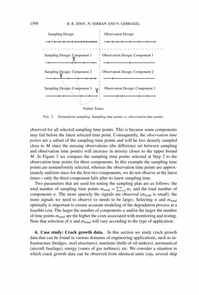
FIG. 3. Nonuniform sampling: Sampling time points vs. observation time points.

observed for all selected sampling time points. This is because some componentsmay fail before the latest selected time point. Consequently, the observation timepoints are a subset of the sampling time points and will be less densely sampledclose to M since the missing observations (the difference set between samplingand observation time points) will increase in density closer to the upper boundM . In Figure 3 we compare the sampling time points selected at Step 2 to theobservation time points for three components. In this example the sampling timepoints are nonuniformly selected, whereas the observation time points are approx-imately uniform since for the first two components, we do not observe at the latesttimes—only the third component fails after its latest sampling time.

Two parameters that are used for tuning the sampling plan are as follows: thetotal number of sampling time points mtotal = ∑n

i=1 mi and the total number ofcomponents n. The more sparsely the signals are observed (mtotal is small), themore signals we need to observe (n needs to be large). Selecting n and mtotaloptimally is important to ensure accurate modeling of the degradation process at afeasible cost. The larger the number of components n and/or the larger the numberof time points mtotal are the higher the costs associated with monitoring and testing.Note that selection of n and mtotal will vary according to the type of application.

6. Case study: Crack growth data. In this section we study crack growthdata that can be found in various domains of engineering applications, such as in-frastructure (bridges, steel structures), maritime (hulls of oil tankers), aeronautical(aircraft fuselage), energy (vanes of gas turbines), etc. We consider a situation inwhich crack growth data can be observed from identical units (say, several ship


hulls, or turbines) up to a predetermined time period, denoted by M in this pa-per. A constant threshold, D, is a critical crack length representing a soft failurewhen maintenance and repair should be performed. Within this context, we assumethat catastrophic failure, that is, hard failure, may occur at a relatively larger cracklength.

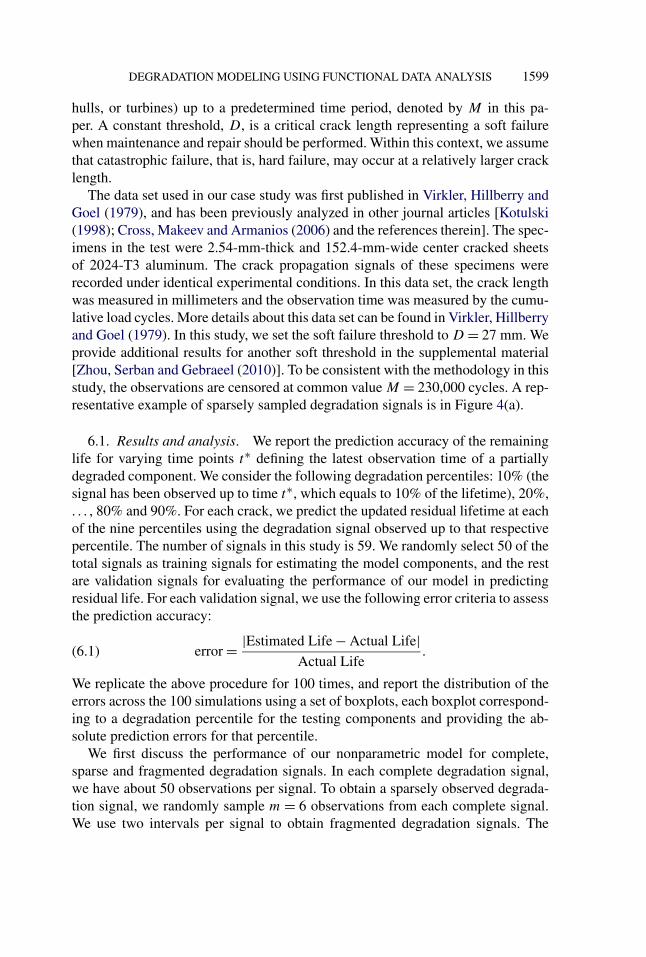
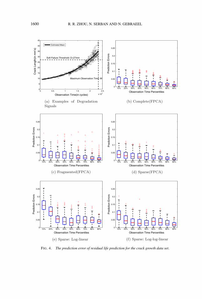
The data set used in our case study was first published in Virkler, Hillberry andGoel (1979), and has been previously analyzed in other journal articles [Kotulski(1998); Cross, Makeev and Armanios (2006) and the references therein]. The spec-imens in the test were 2.54-mm-thick and 152.4-mm-wide center cracked sheetsof 2024-T3 aluminum. The crack propagation signals of these specimens wererecorded under identical experimental conditions. In this data set, the crack lengthwas measured in millimeters and the observation time was measured by the cumu-lative load cycles. More details about this data set can be found in Virkler, Hillberryand Goel (1979). In this study, we set the soft failure threshold to D = 27 mm. Weprovide additional results for another soft threshold in the supplemental material[Zhou, Serban and Gebraeel (2010)]. To be consistent with the methodology in thisstudy, the observations are censored at common value M = 230,000 cycles. A rep-resentative example of sparsely sampled degradation signals is in Figure 4(a).

6.1. Results and analysis. We report the prediction accuracy of the remaininglife for varying time points t∗ defining the latest observation time of a partiallydegraded component. We consider the following degradation percentiles: 10% (thesignal has been observed up to time t∗, which equals to 10% of the lifetime), 20%,. . . , 80% and 90%. For each crack, we predict the updated residual lifetime at eachof the nine percentiles using the degradation signal observed up to that respectivepercentile. The number of signals in this study is 59. We randomly select 50 of thetotal signals as training signals for estimating the model components, and the restare validation signals for evaluating the performance of our model in predictingresidual life. For each validation signal, we use the following error criteria to assessthe prediction accuracy:

error = |Estimated Life − Actual Life|Actual Life

.(6.1)

We replicate the above procedure for 100 times, and report the distribution of theerrors across the 100 simulations using a set of boxplots, each boxplot correspond-ing to a degradation percentile for the testing components and providing the ab-solute prediction errors for that percentile.

We first discuss the performance of our nonparametric model for complete,sparse and fragmented degradation signals. In each complete degradation signal,we have about 50 observations per signal. To obtain a sparsely observed degrada-tion signal, we randomly sample m = 6 observations from each complete signal.We use two intervals per signal to obtain fragmented degradation signals. The


FIG. 4. The prediction error of residual life prediction for the crack growth data set.


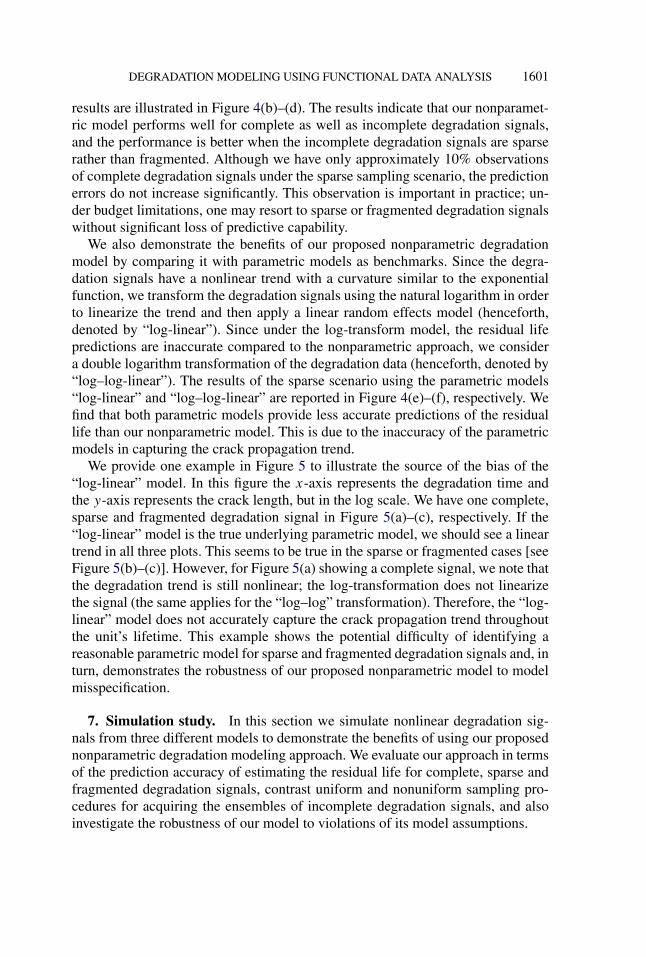
results are illustrated in Figure 4(b)–(d). The results indicate that our nonparamet-ric model performs well for complete as well as incomplete degradation signals,and the performance is better when the incomplete degradation signals are sparserather than fragmented. Although we have only approximately 10% observationsof complete degradation signals under the sparse sampling scenario, the predictionerrors do not increase significantly. This observation is important in practice; un-der budget limitations, one may resort to sparse or fragmented degradation signalswithout significant loss of predictive capability.

We also demonstrate the benefits of our proposed nonparametric degradationmodel by comparing it with parametric models as benchmarks. Since the degra-dation signals have a nonlinear trend with a curvature similar to the exponentialfunction, we transform the degradation signals using the natural logarithm in orderto linearize the trend and then apply a linear random effects model (henceforth,denoted by “log-linear”). Since under the log-transform model, the residual lifepredictions are inaccurate compared to the nonparametric approach, we considera double logarithm transformation of the degradation data (henceforth, denoted by“log–log-linear”). The results of the sparse scenario using the parametric models“log-linear” and “log–log-linear” are reported in Figure 4(e)–(f), respectively. Wefind that both parametric models provide less accurate predictions of the residuallife than our nonparametric model. This is due to the inaccuracy of the parametricmodels in capturing the crack propagation trend.

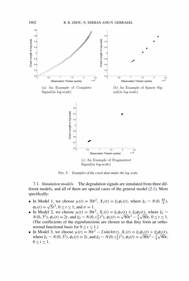
We provide one example in Figure 5 to illustrate the source of the bias of the“log-linear” model. In this figure the x-axis represents the degradation time andthe y-axis represents the crack length, but in the log scale. We have one complete,sparse and fragmented degradation signal in Figure 5(a)–(c), respectively. If the“log-linear” model is the true underlying parametric model, we should see a lineartrend in all three plots. This seems to be true in the sparse or fragmented cases [seeFigure 5(b)–(c)]. However, for Figure 5(a) showing a complete signal, we note thatthe degradation trend is still nonlinear; the log-transformation does not linearizethe signal (the same applies for the “log–log” transformation). Therefore, the “log-linear” model does not accurately capture the crack propagation trend throughoutthe unit’s lifetime. This example shows the potential difficulty of identifying areasonable parametric model for sparse and fragmented degradation signals and, inturn, demonstrates the robustness of our proposed nonparametric model to modelmisspecification.

7. Simulation study. In this section we simulate nonlinear degradation sig-nals from three different models to demonstrate the benefits of using our proposednonparametric degradation modeling approach. We evaluate our approach in termsof the prediction accuracy of estimating the residual life for complete, sparse andfragmented degradation signals, contrast uniform and nonuniform sampling pro-cedures for acquiring the ensembles of incomplete degradation signals, and alsoinvestigate the robustness of our model to violations of its model assumptions.


FIG. 5. Examples of the crack data under the log scale.

7.1. Simulation models. The degradation signals are simulated from three dif-ferent models, and all of them are special cases of the general model (2.1). Morespecifically:

• In Model 1, we choose μ(t) = 30t2, Xi(t) = ξ1φ1(t), where ξ1 ∼ N(0, 454 ),

φ1(t) = √5t2, 0 ≤ t ≤ 1, and σ = 1.

• In Model 2, we choose μ(t) = 30t2, Xi(t) = ξ1φ1(t) + ξ2φ2(t), where ξ1 ∼N(0,32), φ1(t) = 2t , and ξ2 ∼ N(0, (3

2)2), φ2(t) = √80t2 − 3

4

√80t , 0 ≤ t ≤ 1.

(The coefficients of the eigenfunctions are chosen so that they form an ortho-normal functional basis for 0 ≤ t ≤ 1.)

• In Model 3, we choose μ(t) = 30t2 − 2 sin(4πt), Xi(t) = ξ1φ1(t) + ξ2φ2(t),where ξ1 ∼ N(0,32), φ1(t) = 2t , and ξ2 ∼ N(0, (3

2)2), φ2(t) = √80t2− 3

4

√80t ,

0 ≤ t ≤ 1.


We simulate from Model 1 because its residual life distribution can be easilyderived from training signals and updated using validation signals using the pro-cedure in Gebraeel et al. (2005). The derived residual life distribution can then beutilized as a benchmark to assess the performance of our nonparametric approach.

Across all the models, the failure threshold is set to D = 10. We generaten = 100 “training” signals and n = 100 “validation” signals from each model.For a complete signal, we have 51 observations made at an equally spaced gridc0, . . . , c50 on [0,1] with c0 = 0, c50 = 1. A sparse or fragmented signal is thensampled from a complete signal such that we observe about 6 observations persignal. The stopping time for each training signal (the last point at which a sig-nal is observed) is generated from Uniform distribution [Uniform(0.7,1)]—oursimulation results are insensitive to the selection of the stopping time distribution.

We run simulations for 100 times. For each simulation, we compute the predic-tion errors at the following degradation percentiles: 10%, 20%, . . . , 70%, 80% and90% of the simulated degradation signals.

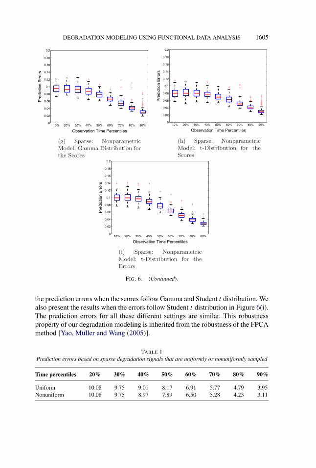
7.1.1. Results and analysis of Model 1. In Figure 6(b)–(d), we present theboxplots of the prediction errors when using the nonparametric degradation modelin this paper for complete, fragmented and sparse degradation signals. For thesparse scenario, we compare the prediction accuracy of using the true parametricmodel [see Figure 6(e)] and our nonparametric model when signals are uniformlysampled [see Figure 6(f)] or nonuniformly sampled [see Figure 6(d)]. We assessthe robustness to model assumptions by simulating signals from the model withξ1 following a Gamma or Student t distribution [see Figure 6(g)–(h)]. We alsocompute the prediction errors under different error distributions [see Figure 6(i)].

The first observation is that there is insignificant difference in the prediction er-rors between the true parametric model and the nonparametric degradation model.The differences are larger for high degradation percentiles. Since the difference inthe prediction errors increases with additional data, we observe for a new compo-nent, we infer that this small inefficiency arises due to a decreased accuracy in theestimation of the empirical prior distribution at the later time points.

The second important observation is that the nonuniform sampling techniqueproposed in Section 5 enhances the prediction accuracy of the residual life. In Ta-ble 1 we list the median prediction errors based on nonuniform sampling and uni-form sampling techniques. The first row of this table represents the time percentileof the degradation signals used for predicting the residual life. It is apparent thatthe nonuniform sampling technique provides smaller prediction errors, especiallyat high time percentiles. This is because nonuniform sampling ensures dense cov-erage of observations over the whole time domain, including the region near max-imum observation time (M), and hence provides more accurate estimate of themean and covariance functions of the model, especially at higher time percentiles.

Last, we assess the robustness to departures from our model assumptions: nor-mality of the scores and normality of the errors. In Figure 6(g)–(h), we compare


FIG. 6. The prediction error of the residual life estimate for Model 1.


FIG. 6. (Continued).

the prediction errors when the scores follow Gamma and Student t distribution. Wealso present the results when the errors follow Student t distribution in Figure 6(i).The prediction errors for all these different settings are similar. This robustnessproperty of our degradation modeling is inherited from the robustness of the FPCAmethod [Yao, Müller and Wang (2005)].

TABLE 1Prediction errors based on sparse degradation signals that are uniformly or nonuniformly sampled

Time percentiles 20% 30% 40% 50% 60% 70% 80% 90%

Uniform 10.08 9.75 9.01 8.17 6.91 5.77 4.79 3.95Nonuniform 10.08 9.75 8.97 7.89 6.50 5.28 4.23 3.11


FIG. 7. Confidence interval estimation: the coverage rate (a) and mean length (b). In each plot theleft and the right bars correspond to the sparse and complete scenarios, respectively.

We also evaluate the accuracy of the confidence interval estimates introducedin Section 4. In Figure 7 we present the coverage rate level and the mean of theconfidence interval length at the degradation lifetime percentiles 50%, 60%, 70%,80% and 90%. The confidence interval level is 1 − α = 0.9. The coverage rateis higher for complete signals than for sparse signals throughout all percentiles,but the difference is insignificant. The coverage rate for both complete and sparsesignals is approximately equal to the confidence level 1 − α = 0.9. Moreover, themean length decreases for higher percentiles, implying that the accuracy of theresidual life estimate increases as the latest observation time point t∗ is closer tothe failure time.

7.1.2. Results and analysis of Model 2. In the following analysis we still useModel 1 as the assumed parametric model and its derived residual life distrib-ution as the benchmark. This assumed parametric model correctly captures themean degradation trend of Model 2 but not the underlying covariance structureof the degradation process. It is worth mentioning that most existing parametricapproaches focus on identification of the functional form for the underlying degra-dation trend, ignoring the underlying covariance structure.

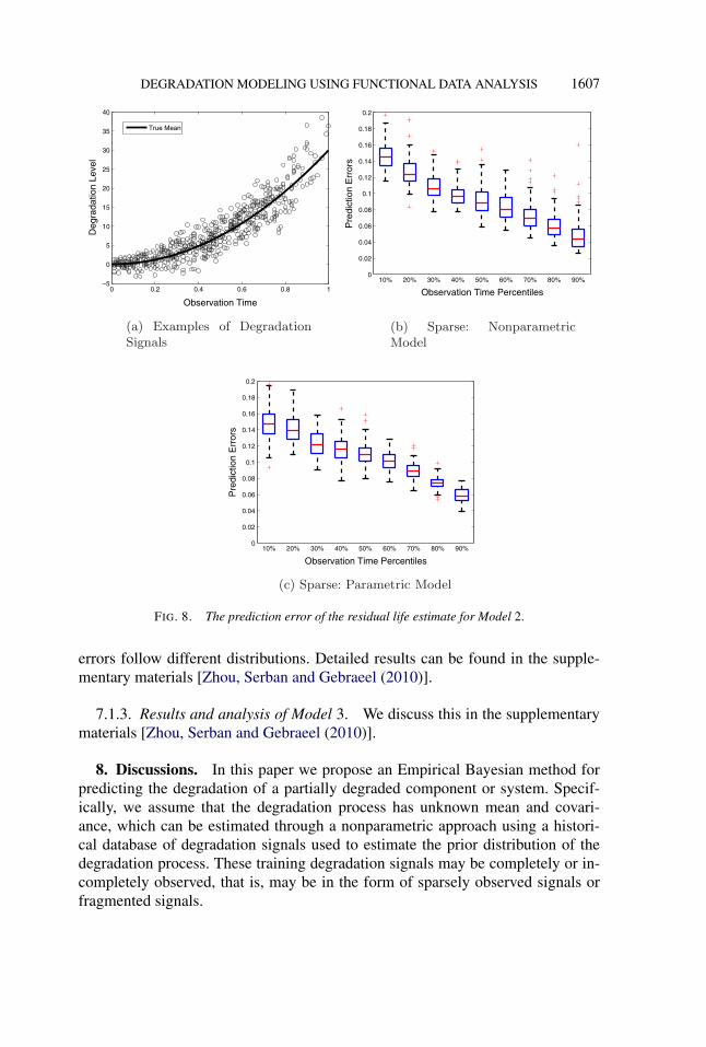
The results in Figure 8 indicate that our nonparametric model is more accuratethan the assumed parametric model in predicting the residual life. This is becauseour proposed nonparametric approach, which is FPCA-based, cannot only estimatethe mean trend accurately but also capture the dominant modes of the covariancestructure correctly. In contrast, parametric models are not flexible enough to accu-rately capture the underlying covariance structure.

We also compute the prediction error results for cases when the observed degra-dation signals are complete, fragmented or sparse, and also when the scores and


FIG. 8. The prediction error of the residual life estimate for Model 2.

errors follow different distributions. Detailed results can be found in the supple-mentary materials [Zhou, Serban and Gebraeel (2010)].

7.1.3. Results and analysis of Model 3. We discuss this in the supplementarymaterials [Zhou, Serban and Gebraeel (2010)].

8. Discussions. In this paper we propose an Empirical Bayesian method forpredicting the degradation of a partially degraded component or system. Specif-ically, we assume that the degradation process has unknown mean and covari-ance, which can be estimated through a nonparametric approach using a histori-cal database of degradation signals used to estimate the prior distribution of thedegradation process. These training degradation signals may be completely or in-completely observed, that is, may be in the form of sparsely observed signals orfragmented signals.


Our degradation modeling and monitoring approach relies on a series of as-sumptions:

• The degradation signals follow a Gaussian process.• The time points at which the training signals have been observed cover the time

domain [0,M] cumulatively.• The degradation signal of the new component does not cross back the thresh-

old D.

From our simulation results, departures from the Gaussian assumption will in-significantly alter the residual life estimates when a large number of training sig-nals are observed, as discussed in Section 7. This property is inherited from therobustness of the FPCA approach used in estimating the empirical prior distribu-tion.

Under sparse sampling, the selection of the observation times of the trainingdegradation signals impacts the accuracy of the degradation prior modeling. Forexample, if the degradation signals are uniformly but sparsely sampled, the degra-dation process will not be adequately observed at the later extreme time point M ,since few components will survive up to this time point. Consequently, uniformsampling compromises the accuracy of the mean and covariance estimates of theprior degradation process, which, in turn, compromises the accuracy of the resid-ual life estimate. In the simulation study we show that the accuracy of the residuallife estimates is low for the traditional uniform sampling as compared to the ac-curacy of the estimates under nonuniform sampling. Thus, the second assumptionis ensured under nonuniform sampling but not uniform sparse sampling (see Sec-tion 5).

The third assumption in our modeling approach relies on that the experimenterwill shut off or replace the component shortly after it degraded beyond the failurethreshold D.

In this paper we have applied the nonparametric approach to crack growth datawith a wide applicability, for example, in infrastructure (bridges, steel structures),maritime (hulls of oil tankers), aeronautical (aircraft fuselage), energy (vanes ofgas turbines) and others. This case study demonstrates the accuracy of the nonpara-metric approach introduced in this paper as compared to random effects parametricmodels which impose constrains on the shape of the trend μ(t) and the covarianceC(t, t ′). Other potential applications are relevant to LED data that could be foundin Yu and Tseng (1998), Liao and Tseng (2006) and Tseng and Peng (2007).

Acknowledgments. We would like to thank the Editor, anonymous AssociateEditor and anonymous reviewers for their constructive and thoughtful commentson this manuscript.


SUPPLEMENTARY MATERIAL

Additional results (DOI: 10.1214/10-AOAS448SUPP; .pdf). In this supple-mental file we provide some additional results of the crack growth data study andthe simulation study.

REFERENCES

BOGDANOFF, J. L. and KOZIN, F. (1985). Probabilistic Models of Cummulative Damage. Wiley,New York.

CROSS, R. J., MAKEEV, A. and ARMANIOS, E. (2006). A comparison of predictions from prob-abilistic crack growth models inferred from Virkler’s data. J. ASTM International 3. DOI:101520/JAI100574.

DAVISON, A. C. and HINKLEY, D. V. (1997). Bootstrap Methods and Their Application. Cam-bridge Series in Statistical and Probabilistic Mathematics 1. Cambridge Univ. Press, Cambridge.MR1478673

DOKSUM, K. A. and HOYLAND, A. (1992). Models for variable-stress accelerated life testing ex-periments based on Wiener processes and the inverse Gaussian distribution. Technometrics 3474–82.

EFRON, B. and TIBSHIRANI, R. J. (1993). An Introduction to the Bootstrap. Monographs on Statis-tics and Applied Probability 57. Chapman and Hall, New York. MR1270903

FAN, J. and YAO, Q. (2003). Nonlinear Time Series: Nonparametric and Parametric Methods.Springer, New York. MR1964455

GEBRAEEL, N. (2006). Sensory updated residual life distribution for components with exponentialdegradation patterns. IEEE Transactions on Automation Science and Engineering 3 382–393.

GEBRAEEL, N., LAWLEY, M., LI, R. and RYAN, J. (2005). Residual-life distributions from compo-nent degradation signals: A Bayesian approach. IIE Transactions 37 543–557.

JAMES, G. M., HASTIE, T. J. and SUGAR, C. A. (2000). Principal component models for sparsefunctional data. Biometrika 87 587–602. MR1789811

KARHUNEN, K. (1947). Über lineare Methoden in der Wahrscheinlichkeitsrechnung. SuomalainenTiedeakatemia, Finland.

KOTULSKI, Z. A. (1998). On efficiency of identification of a stochastic crack propagation modelbased on Virkler experimental data. Archives of Mechanics 5 829–847.

LIAO, C. M. and TSENG, S. T. (2006). Optimal design for step-stress accelerated degradation tests.IEEE Transactions on Reliability 55.

LOÈVE, M. (1945). Functions aleatoire de second order. Comptes Rendus Acad. Sci. 220.LU, C. J. and MEEKER, W. Q. (1993). Using degradation measures to estimate a time-to-failure

distribution. Technometrics 35 161–174. MR1225093MÜLLER, H.-G. and ZHANG, Y. (2005). Time-varying functional regression for predicting remain-

ing lifetime distributions from longitudinal trajectories. Biometrics 61 1064–1075. MR2216200NELSON, W. (1990). Accelerated Testing Statistical Models, Test Plans and Data Analysis. Wiley,

New York.PADGETT, W. J. and TOMLINSON, M. A. (2004). Inference from accelerated degradation and failure

data based on Gaussian process models. Lifetime Data Anal. 10 191–206. MR2081721PARK, C. and PADGETT, W. J. (2006). Stochastic degradation models with several accelerating

variables. IEEE Transactions on Reliability 55 379–390.PETTIT, L. I. and YOUNG, K. D. S. (1999). Bayesian analysis for inverse Gaussian lifetime data

with measures of degradation. J. Statist. Comput. Simulation 63 217–234. MR1703821RAMSAY, J. O. and SILVERMAN, B. W. (1997). Functional Data Analysis. Springer, New York.RICE, J. A. and SILVERMAN, B. W. (1991). Estimating the mean and covariance structure nonpara-

metrically when the data are curves. J. Roy. Statist. Soc. Ser. B 53 233–243. MR1094283

http://dx.doi.org/10.1214/10-AOAS448SUPP

http://dx.doi.org/101520/JAI100574

http://www.ams.org/mathscinet-getitem?mr=1478673










TSENG, S. T. and PENG, C. Y. (2007). Stochastic diffusion modeling of degradation data. J. DataSci. 5 315–333.

VIRKLER, D. A., HILLBERRY, B. M. and GOEL, P. K. (1979). The statistical nature of fatigue crackpropagation. J. Eng. Mater. Technol. 101 148–153.

YAO, F., MÜLLER, H.-G. and WANG, J.-L. (2005). Functional data analysis for sparse longitudinaldata. J. Amer. Statist. Assoc. 100 577–590. MR2160561

YU, H. F. and TSENG, S. T. (1998). On-line procedure for terminating an accelerated degradationtest. Statist. Sinica 8 207–220.

ZHOU, R. R., SERBAN, N. and GEBRAEEL, N. (2010). Supplement to “Degradation modelingapplied to residual lifetime prediction using functional data analysis.” Ann. Appl. Statist. DOI:10.1214/10-AOAS448SUPP.

INDUSTRIAL AND SYSTEMS ENGINEERING

GEORGIA INSTITUTE OF TECHNOLOGY

765 FERST DRIVE, NWATLANTA, GEORGIA 30332-0205USAE-MAIL: [email protected]

[email protected]@isye.gatech.edu


http://dx.doi.org/10.1214/10-AOAS448SUPP

mailto:[email protected]



Degradation modeling applied to residual lifetime …nserban/publications/degradmo… · ·...

Documents

Transcript of Degradation modeling applied to residual lifetime …nserban/publications/degradmo… · ·...