15

D. The Summer Heat Budget The heat budget box model Eq (1) was also applied to MHB during a summer period between 9 August and 11 September 1997. As we will show later, the heating of MHB by the Taunton River is negligible. Therefore, the model we consider is

dHt/dt = ρ cp VMHB dTMHB/dt = (Qair AMHB + dHNBSR/dt +dHBPPS/dt ) . (8) The corresponding temperature equation is TMHB (tn) = [δt/(ρ cp VMHB)] Σn [AMHB Qair(tn) + dHNBSR/dt + dHBPPS/dt(tn)] + TMHB(9Aug) ,

(9) where the assumed values of the other constants is the same as in Eq (7). The following details the measurements that were used to estimate these heat flux components in Eq (8) and thereby the net air-sea heat flux. Qi: The hourly values of incident short-wave solar radiation (obtained from R. Payne, WHOI) show the expectedly clear diurnal cycle (Figure 14).

Figure 14. Hourly incident short-wave solar radiation heat flux measured at Woods Hole, Massachusetts (R. Payne, WHOI).

16

Qb: Measurements of net long-wave radiation to space Qb were not available and needed to be estimated. Qb is proportional to the fourth power of the absolute surface temperature and thus is relatively insensitive to daily-to-seasonal fluctuations of the surface ocean. Therefore, using Mupparapu and Brown (2003) as a guide, Qb was set to the constant value –100 Watts/m2. Qh: The net sensible heat flux is proportional to the wind speed W at 10 m elevation, to the difference of air temperature at 10 m elevation Ta, and to sea surface temperature Ts, which were based on the following.

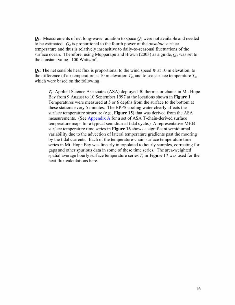
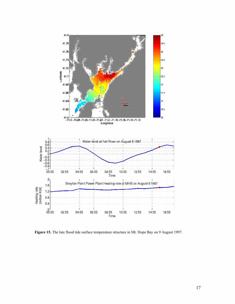
Ts: Applied Science Associates (ASA) deployed 30 thermistor chains in Mt. Hope Bay from 9 August to 10 September 1997 at the locations shown in Figure 1. Temperatures were measured at 5 or 6 depths from the surface to the bottom at these stations every 5 minutes. The BPPS cooling water clearly affects the surface temperature structure (e.g., Figure 15) that was derived from the ASA measurements. (See Appendix A for a set of ASA T-chain-derived surface temperature maps for a typical semidiurnal tidal cycle.) A representative MHB surface temperature time series in Figure 16 shows a significant semidiurnal variability due to the advection of lateral temperature gradients past the mooring by the tidal currents. Each of the temperature-chain surface temperature time series in Mt. Hope Bay was linearly interpolated to hourly samples, correcting for gaps and other spurious data in some of these time series. The area-weighted spatial average hourly surface temperature series Ts in Figure 17 was used for the heat flux calculations here.

17

Figure 15. The late flood tide surface temperature structure in Mt. Hope Bay on 9 August 1997.

18

Figure 16. A ”representative” time series record of surface temperatures in Mt. Hope Bay (located in Figure 1).

Figure 17. The summer 1997 spatially averaged surface temperature in Mt. Hope Bay.

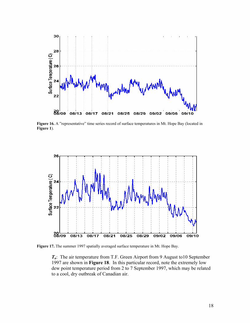
Ta: The air temperature from T.F. Green Airport from 9 August to10 September 1997 are shown in Figure 18. In this particular record, note the extremely low dew point temperature period from 2 to 7 September 1997, which may be related to a cool, dry outbreak of Canadian air.

19

Figure 18. Hourly summer 1997 air temperature at T.F. Green Airport.

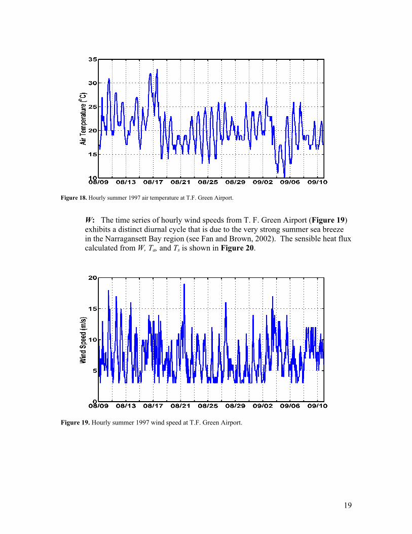
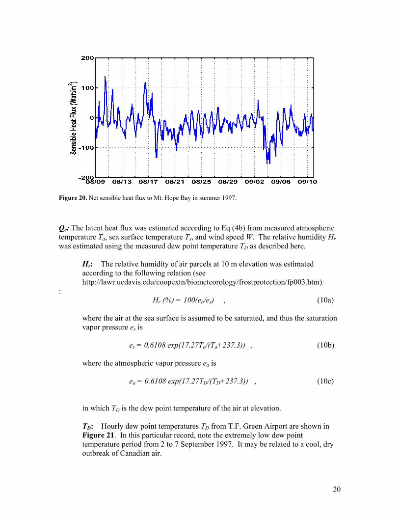
W: The time series of hourly wind speeds from T. F. Green Airport (Figure 19) exhibits a distinct diurnal cycle that is due to the very strong summer sea breeze in the Narragansett Bay region (see Fan and Brown, 2002). The sensible heat flux calculated from W, Ta, and Ts is shown in Figure 20.

Figure 19. Hourly summer 1997 wind speed at T.F. Green Airport.

20

Figure 20. Net sensible heat flux to Mt. Hope Bay in summer 1997. Qe: The latent heat flux was estimated according to Eq (4b) from measured atmospheric temperature Ta, sea surface temperature Ts, and wind speed W. The relative humidity Hr was estimated using the measured dew point temperature TD as described here.

Hr: The relative humidity of air parcels at 10 m elevation was estimated according to the following relation (see http://lawr.ucdavis.edu/coopextn/biometeorology/frostprotection/fp003.htm):

: Hr (%) = 100(ea/es) , (10a)

where the air at the sea surface is assumed to be saturated, and thus the saturation vapor pressure es is

es = 0.6108 exp(17.27Ta/(Ta+237.3)) , (10b)

where the atmospheric vapor pressure ea is

ea = 0.6108 exp(17.27TD/(TD+237.3)) , (10c)

in which TD is the dew point temperature of the air at elevation.

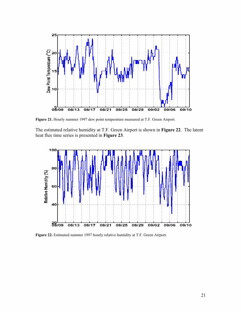
TD: Hourly dew point temperatures TD from T.F. Green Airport are shown in Figure 21. In this particular record, note the extremely low dew point temperature period from 2 to 7 September 1997. It may be related to a cool, dry outbreak of Canadian air.

21

Figure 21. Hourly summer 1997 dew point temperature measured at T.F. Green Airport.

The estimated relative humidity at T.F. Green Airport is shown in Figure 22. The latent heat flux time series is presented in Figure 23.

Figure 22. Estimated summer 1997 hourly relative humidity at T.F. Green Airport.

22

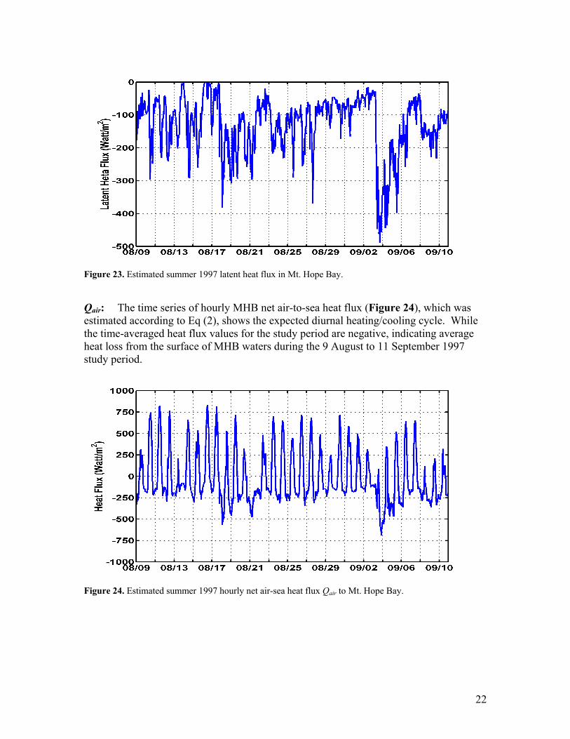
Figure 23. Estimated summer 1997 latent heat flux in Mt. Hope Bay. Qair: The time series of hourly MHB net air-to-sea heat flux (Figure 24), which was estimated according to Eq (2), shows the expected diurnal heating/cooling cycle. While the time-averaged heat flux values for the study period are negative, indicating average heat loss from the surface of MHB waters during the 9 August to 11 September 1997 study period.

Figure 24. Estimated summer 1997 hourly net air-sea heat flux Qair to Mt. Hope Bay.

23

Power Plant Heat Input

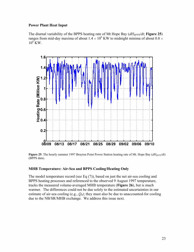
The diurnal variability of the BPPS heating rate of Mt Hope Bay (dHBPPS/dt; Figure 25) ranges from mid-day maxima of about 1.4 H 106 KW to midnight minima of about 0.8 H 106 KW.

Figure 25. The hourly summer 1997 Brayton Point Power Station heating rate of Mt. Hope Bay (dHBPPS/dt) (BPPS data). MHB Temperature: Air-Sea and BPPS Cooling/Heating Only The model temperature record (see Eq (7)), based on just the net air-sea cooling and BPPS heating processes and referenced to the observed 9 August 1997 temperature, tracks the measured volume-averaged MHB temperature (Figure 26), but is much warmer. The differences could not be due solely to the estimated uncertainties in our estimate of air-sea cooling (e.g., Qb); they must also be due to unaccounted-for cooling due to the NB/SR/MHB exchange. We address this issue next.

24

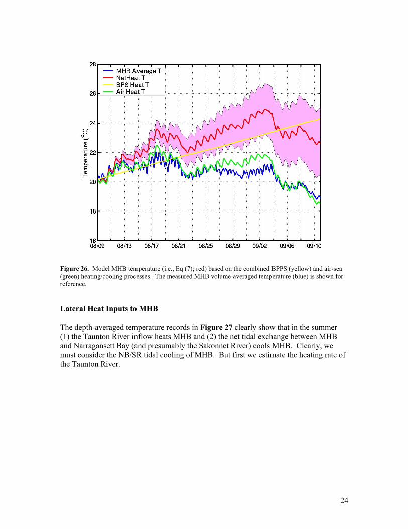
Figure 26. Model MHB temperature (i.e., Eq (7); red) based on the combined BPPS (yellow) and air-sea (green) heating/cooling processes. The measured MHB volume-averaged temperature (blue) is shown for reference. Lateral Heat Inputs to MHB The depth-averaged temperature records in Figure 27 clearly show that in the summer (1) the Taunton River inflow heats MHB and (2) the net tidal exchange between MHB and Narragansett Bay (and presumably the Sakonnet River) cools MHB. Clearly, we must consider the NB/SR tidal cooling of MHB. But first we estimate the heating rate of the Taunton River.

25

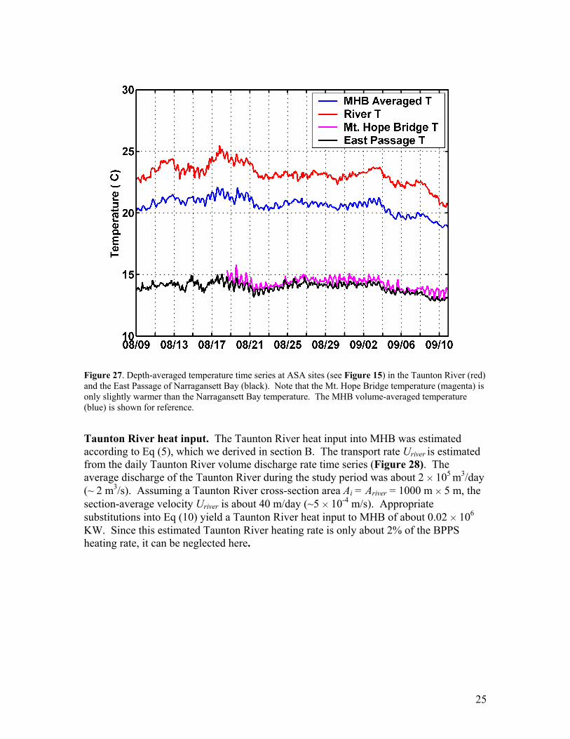
Figure 27. Depth-averaged temperature time series at ASA sites (see Figure 15) in the Taunton River (red) and the East Passage of Narragansett Bay (black). Note that the Mt. Hope Bridge temperature (magenta) is only slightly warmer than the Narragansett Bay temperature. The MHB volume-averaged temperature (blue) is shown for reference. Taunton River heat input. The Taunton River heat input into MHB was estimated according to Eq (5), which we derived in section B. The transport rate Uriver is estimated from the daily Taunton River volume discharge rate time series (Figure 28). The average discharge of the Taunton River during the study period was about 2 H 105 m3/day (~ 2 m3/s). Assuming a Taunton River cross-section area Ai = Ariver = 1000 m H 5 m, the section-average velocity Uriver is about 40 m/day (~5 H 10-4 m/s). Appropriate substitutions into Eq (10) yield a Taunton River heat input to MHB of about 0.02 H 106 KW. Since this estimated Taunton River heating rate is only about 2% of the BPPS heating rate, it can be neglected here.

26

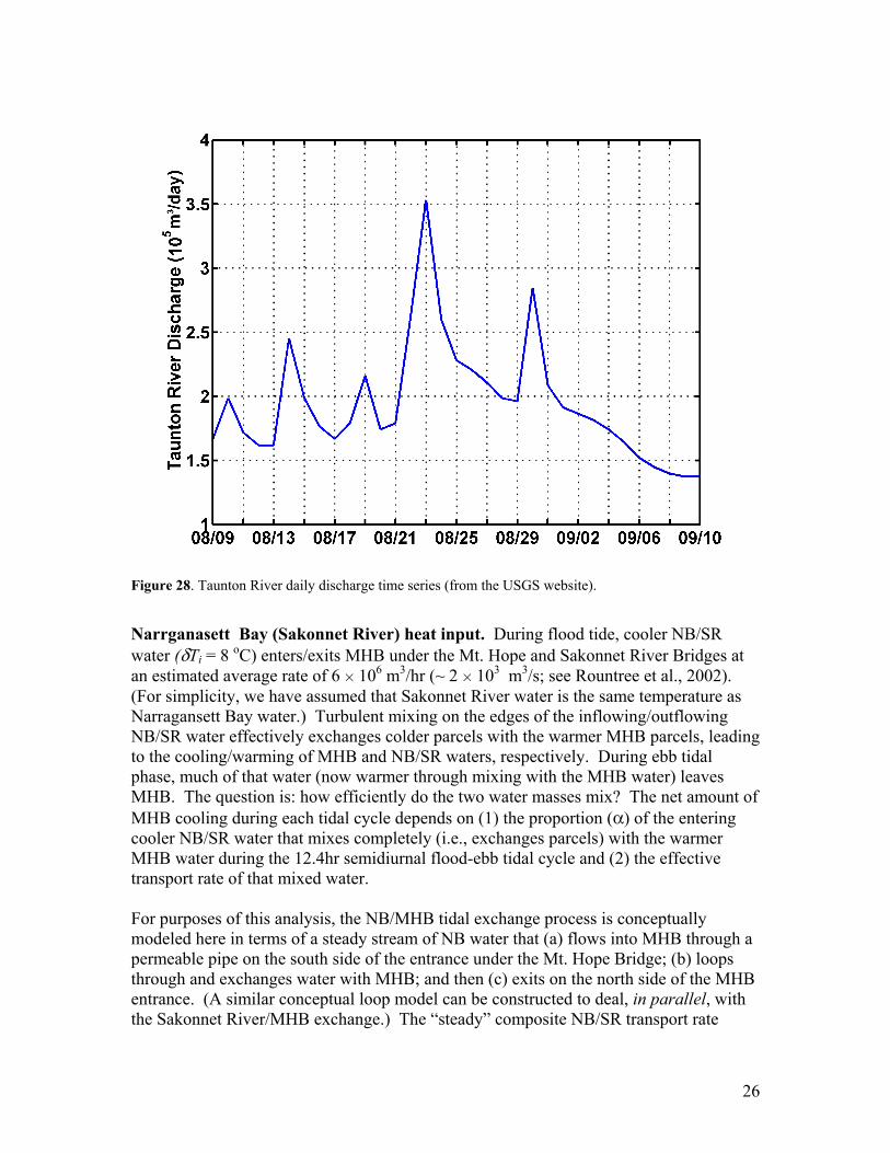
Figure 28. Taunton River daily discharge time series (from the USGS website). Narrganasett Bay (Sakonnet River) heat input. During flood tide, cooler NB/SR water (δTi = 8 oC) enters/exits MHB under the Mt. Hope and Sakonnet River Bridges at an estimated average rate of 6 H 106 m3/hr (~ 2 H 103 m3/s; see Rountree et al., 2002). (For simplicity, we have assumed that Sakonnet River water is the same temperature as Narragansett Bay water.) Turbulent mixing on the edges of the inflowing/outflowing NB/SR water effectively exchanges colder parcels with the warmer MHB parcels, leading to the cooling/warming of MHB and NB/SR waters, respectively. During ebb tidal phase, much of that water (now warmer through mixing with the MHB water) leaves MHB. The question is: how efficiently do the two water masses mix? The net amount of MHB cooling during each tidal cycle depends on (1) the proportion (α) of the entering cooler NB/SR water that mixes completely (i.e., exchanges parcels) with the warmer MHB water during the 12.4hr semidiurnal flood-ebb tidal cycle and (2) the effective transport rate of that mixed water. For purposes of this analysis, the NB/MHB tidal exchange process is conceptually modeled here in terms of a steady stream of NB water that (a) flows into MHB through a permeable pipe on the south side of the entrance under the Mt. Hope Bridge; (b) loops through and exchanges water with MHB; and then (c) exits on the north side of the MHB entrance. (A similar conceptual loop model can be constructed to deal, in parallel, with the Sakonnet River/MHB exchange.) The “steady” composite NB/SR transport rate

27

consistent with the tidal inflow/outflow must be ½ the average tidal inflow/outflow rate or about 103 m3/s.

Figure 29. The “cooling coil” conceptual model of the tidal cooling of MHB during the summer. A steady stream of cool water enters MHB through a semi-permeable pipe that loops into and out of MHB, warming as it exchanges water with the warmer MHB. Thus the heating rate relation for NB/SR tidal exchange cooling is

dHNBSR/dt = α ρ cp UNBSR δTNBSR . (11) Assume for example that, if 5% (α = 0.05) of the entering NB/SR tidal prism water mixes with the MHB waters, then Ui = UNB/SR = 50 m3/s of the cooler NB/SR water enters MHB – effectively replacing the warmer MHB water which exits at the same rate. Then Eq (8) yields a NB/SR heat input to MHB of about -1 H 106 KW – a cooling rate that is of the same order as the BPPS heating rate and needs to be considered.

28

MHB Temperature: Air-Sea and NB/SR Cooling with BPPS Heating Assuming a totally mixed MHB, and heat input from the power plant and exchanges with the Narragansett Bay/Sakonnet River, Eq (1) reduces in this situation to

dHt/dt = ρ cp VMHB dTMHB/dt = (Qair AMHB + dHNBSR/dt +dHBPPS/dt ) , (12) with dHNBSR/dt = α ρ cp UNBSR δTNBSR. The corresponding temperature equation is TMHB (tn) = [δt/(ρ cp VMHB)] Σn [AMHB Qair(tn) + dHNBSR/dt + dHBPPS/dt(tn)] + TMHB(9Aug) ,

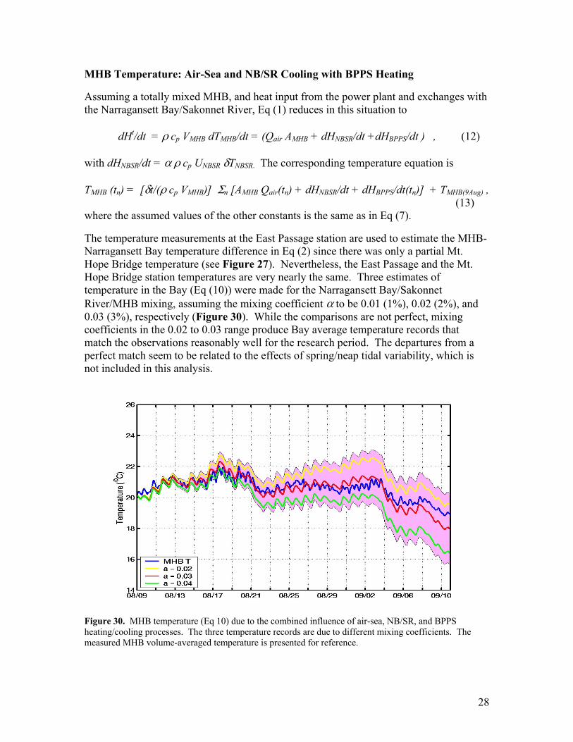
(13) where the assumed values of the other constants is the same as in Eq (7). The temperature measurements at the East Passage station are used to estimate the MHB-Narragansett Bay temperature difference in Eq (2) since there was only a partial Mt. Hope Bridge temperature (see Figure 27). Nevertheless, the East Passage and the Mt. Hope Bridge station temperatures are very nearly the same. Three estimates of temperature in the Bay (Eq (10)) were made for the Narragansett Bay/Sakonnet River/MHB mixing, assuming the mixing coefficient α to be 0.01 (1%), 0.02 (2%), and 0.03 (3%), respectively (Figure 30). While the comparisons are not perfect, mixing coefficients in the 0.02 to 0.03 range produce Bay average temperature records that match the observations reasonably well for the research period. The departures from a perfect match seem to be related to the effects of spring/neap tidal variability, which is not included in this analysis.

Figure 30. MHB temperature (Eq 10) due to the combined influence of air-sea, NB/SR, and BPPS heating/cooling processes. The three temperature records are due to different mixing coefficients. The measured MHB volume-averaged temperature is presented for reference.

29

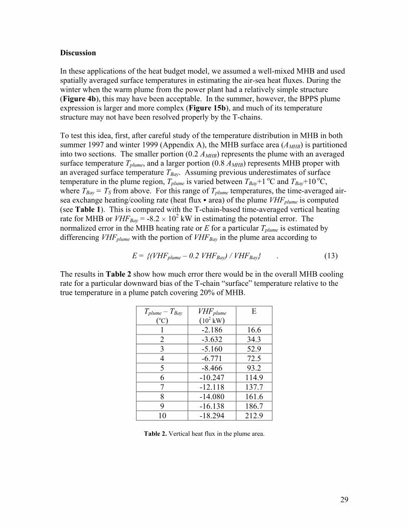
Discussion In these applications of the heat budget model, we assumed a well-mixed MHB and used spatially averaged surface temperatures in estimating the air-sea heat fluxes. During the winter when the warm plume from the power plant had a relatively simple structure (Figure 4b), this may have been acceptable. In the summer, however, the BPPS plume expression is larger and more complex (Figure 15b), and much of its temperature structure may not have been resolved properly by the T-chains. To test this idea, first, after careful study of the temperature distribution in MHB in both summer 1997 and winter 1999 (Appendix A), the MHB surface area (AMHB) is partitioned into two sections. The smaller portion (0.2 AMHB) represents the plume with an averaged surface temperature Tplume, and a larger portion (0.8 AMHB) represents MHB proper with an averaged surface temperature TBay. Assuming previous underestimates of surface temperature in the plume region, Tplume is varied between TBay+1 oC and TBay+10 oC, where TBay = TS from above. For this range of Tplume temperatures, the time-averaged air-sea exchange heating/cooling rate (heat flux C area) of the plume VHFplume is computed (see Table 1). This is compared with the T-chain-based time-averaged vertical heating rate for MHB or VHFBay = -8.2 H 102 kW in estimating the potential error. The normalized error in the MHB heating rate or E for a particular Tplume is estimated by differencing VHFplume with the portion of VHFBay in the plume area according to

E = {(VHFplume – 0.2 VHFBay) / VHFBay} . (13) The results in Table 2 show how much error there would be in the overall MHB cooling rate for a particular downward bias of the T-chain “surface” temperature relative to the true temperature in a plume patch covering 20% of MHB.

Tplume – TBay (oC)

VHFplume (102 kW)

E

1 -2.186 16.6 2 -3.632 34.3 3 -5.160 52.9 4 -6.771 72.5 5 -8.466 93.2 6 -10.247 114.9 7 -12.118 137.7 8 -14.080 161.6 9 -16.138 186.7 10 -18.294 212.9

Table 2. Vertical heat flux in the plume area.

30

This result tells us that exploring spatial structure of air-sea heat loss is very important for the heat budget estimation in MHB, especially during summertime, when the temperature structures in the Bay are very complicated. E. Acknowledgements The research described herein has benefitted from the work of a great many individuals, including Richard E. Payne, who made the short-wave radiation data available to us; our colleagues Lou Goodman, Dan MacDonald, and Zhitao Yu, with whom we have had valuable discussions on this topic; Meredith Simas at Brayton Point Power Station, who provided us with the power station heat input measurements; and Applied Science Associates, Inc, which provided us with the themistor chain measurements. Support for Y.F. was provided by the Brayton Point Power Station.

F. References Beardsley, R.C., E.P. Dever, S.J. Lentz, and J.P. Dean, 1998. Surface heat flux

variability over the northern California shelf, J. Geophys. Res., 103, 21553-21586. Cai, W., and S.J. Codfrey, 1995. Surface heat flux parameterizations and the variability

of thermohaline circulation, J. Geophys. Res., 100(C6), 10,679-10,692. Chinman, R.A., and S.W. Nixon, 1985. Depth-area-volume relationships in Narragansett

Bay, University of Rhode Island Marine Technical Report 87, 64 pp. Edinger , J.E., and J.C. Geyer, 1965. Heat exchange in the environment, in Cooling

Water Discharge Project Report No. 2, Edison Electric Institute Pub. No. 65-902, New York.

Edinger, J.E., D.K. Brady, and J.C. Geyer, 1974. Heat exchange and transport in the environment, in Cooling Water Discharge Project Report No. 14, Electric Power Research Institute Pub. No. 74-049-00-3, Palo Alto, CA.

Edinger, J.E., D.W. Duttweiler, and J.C. Geyer, 1968. The response of water temperature to meteorological conditions, Water Resour. Res., 4, 1137- 1145.

James, I.D., 1977. A model of the annual cycle of temperature in a frontal region of the Celtic Sea, Est. Coast. Mar. Sci., 5, 339-353.

Mustard, J.F., M.A. Carney, and A. Sen, 1999. The use of satellite data to quantify thermal effluent impacts. Est. Coast. Shelf Sci., 49, 509-524.

Rountree, R., D. Borkman, W. Brown, Y. Fan, L. Goodman, B. Howes, B. Rothschild, M. Sundermeyer, and J. Turner, 2002. Franework for formulating the Mt. Hope Bay Natural Laboratory: A synthesis and summary. SMAST Technical Report, School for Marine Science and Technology, University of Massachusetts Dartmouth http://www.smast.umassd.edu/MHBNL/pdffiles/MHBReport0.pdf, 306 pp.

Spaulding, M.L., and F.M. White, 1990. Circulation dynamics in Mount Hope Bay and the lower Taunton River, Coastal and Estuarine Studies, Vol. 38, R.T. Cheng (Ed.), Residual Currents and Long-Term Transport, Springer-Verlag, Inc., New

York.