Proc. NIPR Symp. Polar Meteorol. Glaciol., 9, 146-159, 1995

SEASONAL CHANGE OF THE ATMOSPHERIC HEAT BUDGET OVER

THE SOUTHERN OCEAN FROM ECMWF AND ERBE DATA IN 1988

Itaru 0KADA 1 and Takashi YAMANOUCHI2

1School of Mathematical and Physical Science,

The Graduate University for Advanced Studies,

(National Institute of Polar Research)

9-10, Kaga 1-chome, Itabashi-ku, Tokyo 173 2National Institute of Polar Research,

9-10, Kaga 1-chome, Itabashi-ku, Tokyo 173

Abstract: Seasonal change of the atmospheric heat energy budget in the Antarctic sea ice area in 60 °S-70 °s latitudinal belt in 1988 is obtained from ERBE radiation data and ECMWF global atmospheric data. Seasonal change of the net radiation at the top of the atmosphere, temporal change rate of static energy, convergences of meridional heat energy transport, and the surface heat energy flux are analyzed. To obtain atmospheric heat transport, two methods of correction are adopted. Net radiation at the top of the atmosphere heats the atmosphere in December and January, and cools it in the rest of the year with a negative maximum of -170 W /m2

• The temporal change rate of static energy is positive in the former half of the year and negative in the latter half. Its amplitude is much less than those of other components. Convergences of meridional heat energy transport are uncertain about the yearly averaged level, but their seasonal cycle has two maxima (minima) in April and August (May and October) in which the circumpolar trough is located in higher (lower) latitude and is deeper (shallower) with lag of ± 1 month.

The surface heat energy flux which was obtained as a residual of other terms is maximum in May and minimum in December or January with amplitude of about 200 -230 W /m2

• It takes positive values, at least, during 8 months of the year from March to October. The surface heat flux decreases 33-68 W /m2 from May to July, by which time solar incidence is near zero. Change of cloud amount only cannot explain this reduction. Meanwhile, sea ice concentration increases from 33% to 60%. This increase of sea ice appears to affect to the change of the surface heat flux. In this area, there are few observational data that can be directly compared with the present result. However, by combining observational data and assumptions for radiation term and surface condition, our estimation for the surface heat flux is within the scattering of the observations in autumn.

1. Introduction

The heat budget of the earth has net income at low latitudes and net outgo at high

latitudes. The Southern Ocean is one of the places where a large amount of heat is

released to the atmosphere by the ocean. Meanwhile, sea ice affects surface heat

exchange considerably. An estimation which is obtained by a numerical model offers

area-averaged turbulent heat flux of 56 W /m2, 166 W /m2, and 199 W /m2 when sea ice

concentration is 100%, 65%, and 30%, respectively (WORBY and ALLISON, 1991). For

sensible heat exchange and latent heat exchange at the surface, sea ice acts as an

146

Seasonal Change of the Atmospheric Heat Budget

OE

1 8 0

Fig. 1. Annual variation of sea ice cover. Shaded area shows difference of sea ice cover between September 1986 and February 1987, as being based on 0. 76 of sea ice concentration. Parallels and meridians are drawn every JO degrees. Data are copied by hand from GLOERSEN et al. (1992).

147

insulator between the atmosphere and the ocean. Upward longwave radiation varies from 315 W /m2 to 232 W /m2 corresponding to ocean surface temperature from 0 °C to -20 °C in a simple estimation. Sea ice reduces ocean surface temperature. The albedo of open water is from 0.1 to 0.2, and that of sea ice is from 0.3 to 0. 7 (HIBLER and FLATO, 1989). Figure 1 shows the extent of sea ice, which exhibits a large amplitude for seasonal change in the Southern Ocean. This leads to expect a large variation of the surface heat flux and accompanying changes of atmospheric condition.

There have been few data taken in the Southern Ocean, and remote sensing is difficult. But efforts to estimate surface heat flux using climatology have been made (e.g.,

GORDON, 1981). In this study, net radiation at the top of the atmosphere, convergence of horizontal

heat transport, temporal change rate of static energy, and the surface heat flux as residual are analyzed. The purpose of this study is to offer a spatially averaged atmospheric heat budget, which is derived from global objective analysis atmospheric data and satellite radiation data, and to discuss contributions of sea ice to the surface heat flux.

NAKAMURA and OORT (1988) and MASUDA (1990) estimated the atmospheric heat budget for both polar caps, the area on the polar side of 70 °S/N. NAKMURA and OORT found the seasonal changes of the atmospheric heat budget, using climatology, and MASUDA found the seasonal change, using objective analysis data of the First

148 I. OKADA and T. YAMANOUCHI

GARP Global Experiment. In this study, their method is applied to the 60°S-70

°S

latitude * 360°

longitude "belt". These studies pointed out that horizontal heat transport

includes error in the original the wind field. An effort to avoid the error is made in this

study.

2. Heat Energy Budget

In Fig. 2, the heat energy budget of a unit square atmospheric column is considered.

Let FrnA be the energy flux through the top of the atmosphere, FwALL the energy flux

through the wall integrated from surface (SFC) to the top of the atmosphere (TOA),

and FsFc the energy flux through the land and/or the ocean surface.

A temporal change rate of atmospheric static energy equals the sum of these fluxes:

F To A, F w ALL, and F sFc,

oS/ot = FrnA + FwALL + FsFc. (1)

Sis the sum of atmospheric static energies, consisting of sensible heat energy, latent

heat energy and potential energy integrated from the surface to the top of the atmo­

spheric column,

> --.,,,.,--,,

FwALL = -divE

SENSIBLE HEAT LATENT HEAT POTENTIAL ENERGY

, ,

I

I

I

I

I

:s I I

I

I I

I

I

I

I I

r-

FrnA SHORTWAVE RADIATION LONGW A VE RADIATION

THE TOP OF ----

THE ATMOSPHERE

---- THE SURFACE

SHORTWAVE RADIATION LONGW A VE RADIATION SENSIBLE HEAT LATENT HEAT

8 S/ 8 t = FrnA + FwALL + FsFc

Fig. 2. Heat energy budget of the atmospheric column.

Seasonal Change of the Atmospheric Heat Budget

JTOA

S = ( 1/g)* (CvT+Lq +gZ) dp, SFC

149

(2)

where Cv is specific heat at constant volume (717 J/kg/K), Tis temperature (K), L is latent heat of evaporation (2501 J/g), q is specific humidity (g/kg), g is gravity (9.81 ml s2), and Z is geopotential height.

FrnA is the sum of net longwave radiation and net shortwave radiation,

FrnA = L WNET + SWNET, (3)

where L WNET is longwave net radiation, and SW NET is shortwave net radiation. Net longwave radiation consists of OLR (Outgoing Longwave Radiation) and shortwave net radiation consists of solar incidence and reflected solar radiation.

FwALL = -div E,

FwALL is the convergence of the horizontal energy transport field (E),

fTOA

E= (l/g) * [v* (C p T+Lq+gZ)]dp, • SFC

(4)

where Cp is specific heat at constant pressure ( 1004 J/kg/K), and v is horizontal wind vector. Kinetic energy is ignored here because it is much less than other energies.

Finally, FsFc is obtained as a residual of other terms from the energy budget eq. ( 1). When the surface heat flux is calculated at each grid, the spatial pattern of the flux

obtained tends to depend on the forecast model. In order to eliminate the bias, zonal mean values are adopted in this study.

3. Data Sets

3.1. Data description The ECMWF (European Centre for Medium Range-Weather Forecasts) global

objective analysis data set is used as atmospheric data. This data set is expressed twice-daily in 2.5 degree horizontal grid coordinates and 7 vertical layers (100, 200, 300, 500, 700, 850 and 1000 hPa).

The ERBE (Earth Radiation Budget Experiment) S-4 data set supplied by NASA (National Aeronautics and Space Administration) is used as radiation data. This set includes outgoing longwave radiation and net shortwave radiation at the top of the atmosphere estimated from a narrow field of view radiometer. ERBE was obtained by satellites, NOAA-9, NOAA-10, and ERB-S (Earth Radiation Budget-Satellite). Month­ly data are adopted for this study, and are expressed in 2.5 degree grid coordinates.

3.2. Correction of atmospheric data The prediction model described in sigma-coordinates preserves mass conservation

(MASUDA, 1988; TRENBERTH, 1991). When the data are interpolated from sigma­coordinates to pressure-coordinates, mass conservation is not generally maintained. This

150 I. OKADA and T. YAMANOUCHI

causes a serious error in estimating energy transport. Moreover, the data are inter­polated to obtain vertical integration using a simple spline curve fit in this study. This may also add another error of mass conservation.

In order to eliminate the error, two methods are attempted. In the first method, presented by MASUDA ( 1988) (hereafter, M88), the original wind field was adjusted at each grid point to maintain mass conservation with consideration of global mass distribution.

In the second method, the whole 60 °S-70 °S latitudinal belt is dealt with as a box. Convergence of the horizontal energy transport is calculated in original wind field for the box. Meanwhile, mass convergence is calculated, and the error of energy transport is obtained from the product of the mass convergence and field quantities. The error was maximum (minimum) when it was assumed that the error of mass conservation occurred at the 100 hPa (surface) level at each latitude. This is because of the large

(W /rrf) (a) Radiation budget at the top of the atmosphere 3QQ .-----,-�-,-�.-----,-�-.-�-,---.�-.�.,-----,�-,---,

200

100

0

-100

-200

', ' '

SHORTWAVE RADIATION

,/

,/

LONGW A VE RADIATION

-300'----L�-'-�-'---'-�-'-�-'---'-�-'-�-'-----'�-'-�

(° C) (b) Air temperature -20 .---.�-,-�,----,-�-,--�.,-----,�-.-�.-�.----,-��

-30

J F M A M J J A S O N D

Fig. 3. Zonally averaged fundamental conditions (60°S-70

°S}.

(a) Absorbed shortwave radiation, Outgoing Longwave Radiation, and the net

radiation at the top of the atmosphere which is averaged in the 60°S-70

°S

latitudinal belt.

(b) Temperature which is averaged latitudinally and vertically from the

surface to 100 hPa in the air mass in the 60°S-70

°S latitudinal belt.

Seasonal Change of the Atmospheric Heat Budget 151

contribution of potential energy to total energy. The maximum (minimum) value of estimated error at 70 °S was more (less) than the value at 60 °S as a result, hence, the value at 70°S was adopted to adjust the error of the box. Corrected convergence is obtained by subtracting these errors from the original convergence of the horizontal energy transport. Monthly and zonally averaged data of temperature, potential height, and the mass budget of the box are used for this estimation. Data at the 1000 hPa level are used instead of the data at the surface. This method makes the calculation time very short and is not affected by the error in other areas such as the inner Antarctic continent.

4. Results

Figure 3 shows the annual change of the radiation flux at the top of the atmosphere and air temperature which is averaged by total mass. In the upper part of Fig. 3, the net radiation at the top of the atmosphere shows a minimum in May, June, and July, when solar radiation incidence is near zero. In contrast, the net radiation shows a maximum from December to January when the flux becomes positive. For most of the year, the net radiation cools the atmosphere, changing with shortwave radiation. Longwave radiation

ATMOSPHERIC ENERGY BUDGET (60S-70S) (W/rri')

300���-.-�-,----,�-,-�-.-�,----,-�-.-�-,-�,---,

200

100

0

-100

J F M A M J

* 0 S I () I X frnA

D FwAI.LI • FsFCI

J A S O N D

Fig. 4. Seasonal change of atmospheric heat energy budget. oS/ot: temporal change rate of statical heat energy of atmosphere, FroA: net heat energy flux at the top of the atmosphere, FwALLJ: convergence of meridional heat energy transport which is obtained using the correction method MASUDA (1988),

F WALL2A: convergence of meridional heat energy transport which is locally corrected and gives the maximum value, FwALL2B: same as FwALL2A except minimum value, FsFcJ: net heat energy flux at the surface which is obtained as a residual from oS/ ot, Fro...t, and FwALLJ, FsFC2A: same as FsFCI except FwALL2A, FsFcw: same as FsFcJ except FwALL2B·

152 I. OKADA and T. y AMANOUCHI

changes with the amplitude of about 20 W /m2 • Heat loss by longwave radiation becomes a minimum in winter. Air temperature takes its maximum and minimum in January and July, as shown in the lower part of Fig. 3.

Figure 4 shows seasonal changes of net radiation flux at the top of the atmosphere, convergence of horizontal energy transport, temporal change rate of static energy, and the surface energy flux. Flux flowing into the atmosphere is expressed by positive values.

The temporal change rate of static energy varies with the amplitude of about 22 W / m2, with positive values from August to December, and negative values from January to July. Variations of the rate are much smaller than other terms such as FrnA, FwALL, and FsFc. The air temperature decreases slowly from January to July, and increases rapidly from September to December. The temporal change rate of static energy correlates with the change rate of temperature.

In Fig. 4, convergence of horizontal heat energy transport appears as 3 curves, corresponding to the two kinds of mass correction method as mentioned in Section 3. The averaged values are different from each other but the patterns of their seasonal variations are similar. Both convergences take maxima in April and August, and minima in May, and in October or November, with amplitudes of about 66-95 W /m2

•

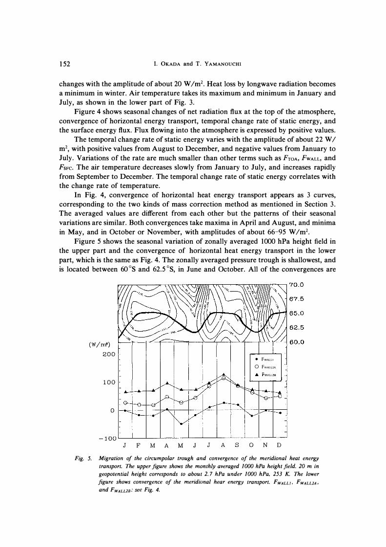
Figure 5 shows the seasonal variation of zonally averaged 1000 hPa height field in the upper part and the convergence of horizontal heat energy transport in the lower part, which is the same as Fig. 4. The zonally averaged pressure trough is shallowest, and is located between 60 °S and 62.5 °S, in June and October. All of the convergences are

(W /rrr)

200

100

0

J F M A M J

• FwALLJ

0 FwALL2A

J A S O N D

Fig. 5. Migration of the circumpolar trough and convergence of the meridional heat energy transport. The upper figure shows the monthly averaged 1000 hPa height field. 20 m in geopotential height corresponds to about 2. 7 hPa under 1000 hPa, 253 K. The lower figure shows convergence of the meridional hear energy transport. F WALL/, F WALL2A,

and F WALL2B: see Fig. 4.

Seasonal Change of the Atmospheric Heat Budget 153

minimum in May, and FwALLI is minimum in October. In contrast, the trough is deeper and located near 65 °S in March, July, and December. All of the convergences are maxima in April and August. Migration and depth of the pressure trough show curves similar to the convergences. The typical phase of the semi annual oscillation (SAO) shows that the trough is located in highest latitude in March and October (e.g., VAN

LOON, 1967). This is different from 1988, and suggests that the SAO has a large variation in interannual time scale.

As seen in Fig. 4, the surface fluxes are positive in most seasons, increasing rapidly from January to May, and decreasing slowly from May to December. From May to July, the surface fluxes decrease about 33-68 W /m2

, although shortwave radiation flux is almost stable and near zero in the same period as shown in Fig. 3. In summer, the surface fluxes are minimum in December and January, and shortwave radiation flux is also maximum in the same months, greatly different from November and February.

5. Discussion

The area of investigation in this study includes the continental region. This region is approximate by 10% of the total area, and almost covered by the ice shelf all year. Thus it may affect the bias level of the surface flux but not that of the variational part. Meanwhile, as seen in Fig. 1, there is always some open sea, and sea ice is distributed inhomogeniously in the area. This condition may have a different effect on the heat exchange from the condition of uniformly distributed sea ice. This is a subject that should be considered in further studies, and not discussed in detail here.

Figure 6 shows the surface heat flux over open sea which was estimated by

SURFACE ENERGY BUDGET (60S-70S) (W /rri')

300rr""""'=====::a================.:=========-==,-,

200

100

0

-100

e NET LONGW A VE RADIATION FLUX • TOT AL FLUX

& NET SHORTWAVE RADIATION FLUX A SENSIBLE HEAT FLUX

0 LA TENT HEAT FLUX

J F M A M J J A S O N D

Fig. 6. Surface energy budget. Fluxes of sensible heat, latent heat, shortwave radiation,

and longwave radiation which are estimated by climatological data for open sea

conditions (GORDON, 1981).

1 54 I. OKADA and T. YAMANOUCHI

GORDON (198 1) . From May to July, the shortwave radiation flux is near O W /m2, and

the longwave radiation flux is almost stable. In the same period, the sensible heat flux and the latent heat flux increase. As a result, the total flux at the surface increases in this period. However, the present result of the surface flux shown in Fig. 5 decreases 33-68 W /m2, opposite to the expected tendency as shown above.

The surface heat flux should be affected by clouds and sea ice. Increase of cloud amount decreases surface heat flux. The longwave part of the difference between flux with cloud cover of 10 and the flux with clear sky is estimated to be 52 W /m2 at Syowa Station (YAMANOUCHI and CHARLOCK, 1995) . Thus the cloud amount must increase more than 6/10 to reduce the surface heat flux by 33 W /m2, which is the difference between May and July as seen in Fig. 5. Several estimations have been made of the cloud climatology as ISCCP (Rossow and GARDER, 1 993), though there are no reliable estimates of cloud cover distribution in this area. At least, cloud amount is large throughout the year. Actually, frequency of cloudy sky (cloud amount of 6/8-8/8) is 85% and 90% in winter and summer, respectively, according to ELTANIN cruises (table 5 .7. of SCHWERDTFEGER, 1984) . And monthly means of cloud amount at Syowa Station are 7. 6 (May) and 6. 3 (July) in 1988 (JAPAN METEOROLOGICAL AGENCY, 1990) . Definitely cloud is not the primary factor for the decrease of the surface heat flux in this case.

Meanwhile, as explained in Section 1, sea ice works as a suppressor in terms of sensible heat, latent heat, and longwave radiation. Figure 7 shows the change of sea ice concentration averaged in the 60 °S-70 °S latitudinal belt, based on data distributed by NSIDC (National Snow and Ice Data Center) as a value at the end of each month in rectangular equal-area grids. As seen in Fig. 7, sea ice concentration increases from 33% (May) to 60% (July) . The present result suggests that sea ice plays a major role in decreasing the surface heat flux in this period. In autumn and spring, the role of sea ice

( % )

1 00

80

60

40

20

0

SEA ICE C(?NCENTRATION (60S-70S)

/ ---------... -

/

I \ /

--/

J F M A M J J A S O N D

Fig. 7. Seasonal change of sea ice concentration. The data were averaged in the 60 °S-70 °S latitudinal belt. A value in each month shows data at the end of the month in 1988.

Seasonal Change of the Atmospheric Heat Budget 155

in reducing the surface flux cannot be discussed from these data, because a large change of downward shortwave radiation veils the effect of sea ice on the surface flux.

In summer, global solar radiation at the surface largely varies from month to month (e.g. 350.2 W /m2 in December and 167.4 W /m2 in February at Syowa Station, JAPAN METEOROLOGICAL AGENCY, 1990), and sea ice concentration changes from 21 % at the end of December to 5% at minimum at the end of February. The increase of the surface heat flux, which is caused by this decrease of albedo, is smaller than the change of global solar radiation which decreases to about half from December to February. Hence the curve of the surface heat flux is dominated by change of downward shortwave radiation at the surface.

Change of cyclone activity with SAO has already been reported in several papers (e.g. CARLETON, 1981). The present result suggests that cyclone activity has some connection with the surface heat flux because of the relationship between the location of the trough and the convergence of the meridional heat transport. Cyclone activity contributes to increase turbulent flux at the ocean surface (ZILLMAN, 1972). However, in the present result, cyclone activity increases and the surface flux decreases when the convergence increases, from eq. (1). Though this difference may be induced by the spatial/time scale of the phenomenon and/or the radiation term, further study of these correlations, may show that some interaction between atmosphere, ocean and sea ice is involved.

The meridional heat energy transport can be separated into two terms, which are the mean meridional circulation (MMC) and the eddy term (e.g., PEIXOTO and OORT, 1992). The phases and amplitudes of seasonal change of the convergences which are obtained from the present result are very similar each other, and the seasonal change of the convergences corresponds to migration of the trough. Hence the seasonal change of the convergences may correspond to the eddy term, and yearly averaged level of convergences as the remainder may correspond to the MMC. This suggests that the method of mass correction influences estimation of the MMC.

6. Comparison of the Present Results and Observations

Figure 8 shows surface heat fluxes from the present results, other estimations, and observations. The seasonal change of our results resembles the estimation of GORDON (1981). This similarity has its origin in the large amplitude of downward shortwave radiation at the surface. A remarkable similarity is the positive peaks in early winter. Several observations have been reported (KANGOS, 1960; RAMESH KUMAR and GAN­GADHARA RAO, 1989; VIEBROCK, 1962; ZILLMAN, 1972). Most of them are observa­tions of sensible heat and latent heat on the open sea. WELLER ( 1980) applied the model of MAYKUT (1978) to estimate sensible heat flux and latent heat flux for the pack ice zone.

In summer, data of the observations are concentrated in the smallest range of flux. Total flux consists of a larger amount of shortwave radiation flux (negative) and smaller amount of sum of longwave radiation, sensible heat and latent heat flux (positive). Thus the present result and the estimation of GORDON ( 1981) take negative values. The range of fluxes is wider in autumn and spring. The extent of the range suggests difficulty in

156

(W /rrf) 200

1 00 K606

K6570 V6570 Z6468 Z6064

5 �

�

0

- 1 0 0

�

�' V6065

I. OKADA and T. YAMANOUCHI

sensible heat and latent heat flux

' ' Wl IV657o *

IK.6570 -W2

�1

60�i -657 IZ6064 -I V6065

I - V6065 -

Z6064 Z6064 ' I -

Z6468 - - RG T

RG

total heat flux 300 �������������������....--------��

J

a FsFc1

J;. FsFc2A

e FsH'2B

F M A M J J A s O N D

Fig. 8. Observed and estimated surface heat fluxes. The upper figure shows the sum of sensible heat and latent heat fluxes. The lower figure shows the total flux. The shaded area in the upper figure exhibits maxima and minima of total flux according to the present result in each month. Wl: sensible heat and latent heat estimated by the model calculation with sea ice concentration of more than 15 % and less than 85% (WELLER, 1980), W2: same as Wl except more than 85 % of sea ice concentration, V6065: sensible heat and latent heat over the open sea, presenting values in the 60 °S-65 °S latitudinal belt (VIEBROCK, 1962), V6570: same as V6065 except 65 °S-70 °S, K6065: sensible heat and latent heat over open sea, presenting values in the 60 °S-65 °S latitudinal belt (KANGOS, 1960), K6570: same as K6065 except 65 °S-70 °S, Z6064: sensible heat and latent heat over the open sea, presenting values in the 60 °S-63. 9 °S (ZILLMAN, 1972), Z6468: same as Z6064 except 64 °S-67. 9 °S, and RG: sensible heat and latent heat observed in the southern Indian Ocean (RAMSH K uMAR and GANGADHARA RAO, 1989). Horizontal thin solid lines show average of 3 months except RG. •: V6570 in spring presents data in the Ross Sea. G81: total flux of GORDON (1981) obtained from climatology with realistic sea ice concentration, GH: heat flux under sea ice in the Weddell Sea mixed layer (GORDON and HUBER, 1990). FsFcJ , FsFC 2A , and FsFc 2B: see Fig. 4.

Seasonal Change of the Atmospheric Heat Budget 157

attaching significance to spatially averaged properties. In autumn, the present result stays almost in the range of observations. The global

solar incidence at Syowa Station (69 °S), which offers 75.2 W /m2 in March (JAPAN METEOROLOGICAL AGENCY, 1990), sets the net radiative flux near O W /m2

• This means that only sensible heat and latent heat fluxes appear in the value of the total flux. And the ocean surface is close to open sea, because sea ice concentration shows about 5% in March, as s,een in Fig. 7. These conditions for radiation and surface make direct comparison between our estimation for total flux and observations for sensible heat and latent heat fluxes on the open sea possible. The results of simplified correction (FsFciA, FsFc2B) take similar values with the estimation of G8 l. The average of the result by the M88 method (FsFc t) in MAM is the mostly same as observation at 65 °S-70 °S latitudes by KANGOS (1960). Thus the present result, which does not appear radiation terms, is also generally similar to observations.

In winter, heat flux in the ocean mixed layer, which is observed under sea ice in the Weddell Sea, is 41 W /m2 (GORDON and HUBER, 1990) (hereafter GH). This heat is consumed by transfer mostly to the atmosphere and melting sea ice. The surface flux takes a value just under the flux in the ocean mixed layer. The estimation of WELLER (1980) in the inner pack ice zone exceeds the observation of ZILLMAN (1972) (hereafter Z72) in the open sea. This relationship shows that the spatial difference of the surface heat exchange is so large due to the local condition. Results of simplified mass budget correction (FsFc2A, FsFc2B) are slightly upper values than GH which may be a minimum value in the data for the latitudinal belt, and values lower than Z72 which consists of sensible heat and latent heat. The present result by the M88 method (FsFc1) is higher than Z72 and lower than the value of WELLER ( 1980), assuming the ice concentration of 15-85%.

In spring, the result of simplified correction (FsFc2A, FsFc2B) and the estimation of G81 are approximately the same or lower than observations except the highest one. The present result by the M88 (FsFct) method takes a larger value than these two observa­tions. Due to extended sea ice, the average surface condition of this belt is far from open sea. These observations may be rather minor examples.

The mean of the observed surface flux which consists of sensible heat and latent heat in autumn is significantly larger (positive) than in summer. The total flux according to the present result in autumn is also larger than in summer, but it does not always reflect sensible heat and latent heat. The total surface flux generally depends on downward shortwave radiation, thus the present result can appear to be within the scatter of observations with certain assumptions for radiation. It is difficult to determine whether the present result agrees with observed data or not, because most of the observations show sensible heat and latent heat fluxes which change with smaller amplitude than the downward shortwave radiation, and because these observations are restricted in the case over open sea.

7. Summary and Concluding Remarks

The seasonal change of the atmospheric heat energy budget in 1988 was obtained from a global objective analysis data set and radiation data set over the Southern Ocean,

158 I. OKADA and T. YAMANOUCHI

60 °S-70 °S latitudinal belt. To obtain the horizontal energy transport, two kinds of mass correction are adopted. Net radiation at the top of the atmosphere heats the atmosphere in December and January, and cools it in the rest of the year with a negative maximum of -170 W /m2

• The temporal change rate of static energy is positive in the former half of the year and negative in the latter half. Its amplitude is much less than other component. Convergences of horizontal heat energy transport are uncertain for the yearly average. These averages depend on the correction method, which may affect the MMC components. Patterns of seasonal cycle of the convergences are similar and take maxima at the same times, in April and August. The surface heat energy flux is maximum in May and minimum in December or January. The amplitude is about 200 -230 W /m2

• It takes positive values from April to November in both methods. The surface flux decrease 33-68 W /m2 from May to July in which solar incidence

is near zero. This change is too large for reduction by increased cloud amount. In this period, sea ice concentration increases from 33% to 60%. This suggests that sea ice acts as a heat insulator to the surface flux. The convergence of meridional heat transport increases (decreases) when the circumpolar trough is located to the south (north) and is deeper (shallower) with a lag of + 1 month. This relation suggests that the surface flux has some connection with the meridional heat transport through cyclone activity and the surface condition. More cases for other years need to be investigated to obtain a more definite result.

The present result is compared with field observations which consist of sensible heat and latent heat on the open sea in most cases. All of the observations take positive values in summer. The present result and the observations appear to be similar in autumn, though the interpretation depends on assumptions for the radiation terms. Cases in winter are few, but the present results equal or exceed the total flux in the ocean mixed layer in the Weddell Sea.

Acknowledgments

The authors are grateful to N. HIRASAWA, National Institute of Polar Research, for useful discussions as a referee, and to K. MASUDA, Department of Geography, Tokyo Metropolitan University, for comments as a referee and a suggestion about calculation. Comments from an anonymous referee improved the article. The authors thank to ECMWF, NASA, and NSIDC for providing data. The HIT AC M-680D in the Information Science Center of NIPR was used. FISHPACK and NCARG, which were produced by the National Center for Atmospheric Research, were used for calculations and drawings.

References

CARLTON, A.M. ( 1981) : Monthly variability of satellite-derived cyclonic activity for the southern hemisphere winter. J. Climatol. , 1, 21-38.

GORDON, A.L. (1981) : Seasonality of southern ocean sea ice. J. Geophys. Res., 86, 4193-4197. GORDON, A.L. and HUBER, B.A. (1990) : Southern ocean winter mixed layer. J. Geophys. Res., 95, 11655-

11672.

Seasonal Change of the Atmospheric Heat Budget 1 59

GLOERSEN, P., CAMPBELL, W.J., CAVALIERI, D.J. , COMISO, J.C., PARKINSON, C.L . and ZwALLY, H .J. ( 1992): Arctic and Antarctic sea ice, 1978- 1 987: Satellite passive-microwave observations and analysis. Washington, D.C., NASA, 290p.

HIBLER, W.D., Ill and FLATO, G.M. ( 1989) : Sea ice models. Climate System Modeling, ed. by K.E. TRENBERTH. Cambridge, Cambridge Univ. Press, 414.

JAPAN METEOROLOGICAL AGENCY ( 1 990) : Meteorological data at the Syowa Station in 1988. Antarct . Meteorol. Data, 29, 326p.

KANGOS, J.D. ( 1960) : A preliminary investigation of the heat flux from the ocean to the atmosphere in Antarctic regions. J. Geophys. Res . , 65, 4007-4012 .

MASUDA, K. ( 1988) : Meridional heat transport by the atmosphere and the ocean: analysis of FGGE data. Tellus, 40A, 285-302.

MASUDA, K. ( 1990) : Atmospheric heat and water budgets of polar regions: Analysis of FGGE data. Proc . NIPR Symp. Polar Meteorol. Glaciol . , 3, 79-88.

MAYKUT, G.A. ( 1978) : Energy exchange over young sea ice in the central Arctic ., J . Geophys. Res., 83, 3646 -3658 .

NAKAMURA, N . and OORT, A.H. ( 1 988) : Atmospheric heat budgets of the polar regions, J . Geophys. Res. , 93, 95 10-9524.

PEIXOTO, J.P and OORT, A.H. ( 1992) : Physics of Climate. New York, American Institute of Physics, 61 -64. RAMESH KUMAR, M.R. and GANGADHARA RAO, L.V. ( 1 989) : Latitudinal variation of air sea fluxes in the

western Indian Ocean during austral summer and fall. Boundary-Layer Meteorol . , 48, 99- 107. Rossow, W.B. and GARDER, L.C. ( 1993) : Validation of ISCCP cloud detections, J. Clim., 6, 2370-2393 . SCHWERDTFEGER, W. ( 1984) : Weather and Climate of the Antarctic. Amsterdam, Elsevier, l 79p. (Develop­

ments in Atmospheric Science, 1 5) . TRENBERTH, K.E. ( 199 1 ) : Climate diagnostics from global analyses: Conservation of mass in ECMWF

analyses. J. Clim., 4, 707-722. VAN LooN, H. ( 1967) : The half-yearly oscillations in middle and high southern latitudes and the coreless

winter. J. Atmos . Sci ., 24, 472-486. VIEBROCK, H. ( 1962) : The transfer of energy between the ocean and the atmosphere in the Antarctic region.

J. Geophys. Res., 67, 4293-4302. WELLER, G. ( 1980) : Spatial and temporal variations in the south polar surface energy balance. Mon. Weather

Rev., 108, 2006-2014. WORBY, A.P. and ALLISON, I. ( 1 99 1 ) : Ocean-atmosphere energy exchange over thin, variable concentration

Antarctic pack ice. Ann . Glaciol., 15, 184- 190. YAMANOUCHI, T. and CHARLOCK, T.P. ( 1 995) : Comparison of radiation budget at the TOA and surface in

the Antarctic from ERBE and ground surface measurements. to published in J. Clim. ZILLMAN, J.W. ( 1972) : Solar radiation and sea-air interaction south of Australia. Antarctic Oceanology II ,

ed. by D.E. HAYES. Washington, D.C., Am. Geophys. Union, 1 1 -40 (Antarct. Res. Monogr. No. 19) .

(Received April 24, 1995; Revised manuscript received June 6, 1995)