cover new impa ceris 2010 - Stata · cover new impa ceris 2010 26-01-2010 7:36 Pagina 1. l\rWorking...

$: cover new impa ceris 2010 - Stata · cover new impa ceris 2010 26-01-2010 7:36 Pagina 1. l\rWorking paper Cnr-Ceris, N.04/2014\rl\rIDENTIFICATION AND ESTIMATION \rOF TREATMENT EFFECTS$
WorkingPaperWorkingPaper

ISTITUTO DI RICERCASULL’IMPRESA E LO SVILUPPO

ISSN (print): 1591-0709ISSN (on line): 2036-8216

Co

nsi

gli

o N

azio

na

le d

ell

e R

ice

rch

e

cover new impa ceris 2010 26-01-2010 7:36 Pagina 1

e.viarisio

Casella di testo

l Working paper Cnr-Ceris, N.04/2014 l IDENTIFICATION AND ESTIMATION OF TREATMENT EFFECTS IN THE PRESENCE OF NEIGHBOURHOOD INTERACTIONS l Giovanni Cerulli

Cerulli G., Working Paper Cnr-Ceris, N° 04/2014

Copyright © 2014 by Cnr-Ceris All rights reserved. Parts of this paper may be reproduced with the permission of the author(s) and quoting the source.

Tutti i diritti riservati. Parti di quest’articolo possono essere riprodotte previa autorizzazione citando la fonte.

WORKING PAPER CNR - CERIS

RIVISTA SOGGETTA A REFERAGGIO INTERNO ED ESTERNO

ANNO 16, N° 4 – 2014 Autorizzazione del Tribunale di Torino

N. 2681 del 28 marzo 1977

ISSN (print): 1591-0709

ISSN (on line): 2036-8216

DIRETTORE RESPONSABILE

Secondo Rolfo

DIREZIONE E REDAZIONE

Cnr-Ceris

Via Real Collegio, 30

10024 Moncalieri (Torino), Italy

Tel. +39 011 6824.911

Fax +39 011 6824.966

[email protected]

www.ceris.cnr.it

COMITATO SCIENTIFICO

Secondo Rolfo

Giuseppe Calabrese

Elena Ragazzi

Maurizio Rocchi

Giampaolo Vitali

Roberto Zoboli

SEDE DI ROMA

Via dei Taurini, 19

00185 Roma, Italy

Tel. +39 06 49937810

Fax +39 06 49937884

SEDE DI MILANO

Via Bassini, 15

20121 Milano, Italy

tel. +39 02 23699501

Fax +39 02 23699530

SEGRETERIA DI REDAZIONE

Enrico Viarisio

[email protected]

DISTRIBUZIONE

On line:

www.ceris.cnr.it/index.php?option=com_content&task=section&id=4&Itemid=64

FOTOCOMPOSIZIONE E IMPAGINAZIONE

In proprio

Finito di stampare nel mese di Marzo 2014

mailto:[email protected]


Identification and Estimation

of Treatment Effects in the Presence

of Neighbourhood Interactions

Giovanni Cerulli

CNR - National Research Council of Italy

CERIS - Institute for Economic Research on Firm and Growth

Via dei Taurini 19, 00185 Roma, ITALY

Mail: [email protected]

Tel.: 06-49937867

ABSTRACT: This paper presents a parametric counter-factual model identifying Average

Treatment Effects (ATEs) by Conditional Mean Independence when externality (or

neighbourhood) effects are incorporated within the traditional Rubin’s potential outcome model.

As such, it tries to generalize the usual control-function regression, widely used in program

evaluation and epidemiology, when SUTVA (i.e. Stable Unit Treatment Value Assumption) is

relaxed. As by-product, the paper presents also ntreatreg, an author-written Stata routine for

estimating ATEs when social interaction may be present. Finally, an instructional application of

the model and of its Stata implementation through two examples (the first on the effect of

housing location on crime; the second on the effect of education on fertility), are showed and

results compared with a no-interaction setting.

Keywords: ATEs, Rubin’s causal model, SUTVA, neighbourhood effects, Stata command.

JEL Codes: C21, C31, C87

An early version of this paper was presented at CEMMAP (Centre for Microdata Methods and Practice), University

College London, on March 27th 2013. The author wishes to thank all the participants to the seminar and in particular

Richard Blundell, Andrew Chesher, Charles Manski, Adam Rosen and Barbara Sianesi for the useful discussion. This

version of the paper has been presented at the Department of Economics, Boston College, on November 12 th 2013.

The author wishes to thank all the participants to the seminar and in particular Kit Baum, Andrew Beauchamp,

Rossella Calvi, Federico Mantovanelli, Scott Fulford and Mathis Wagner for their participation and suggestions.



4

CONTENTS

1. Introduction .............................................................................................................................. 5

2. Related literature ...................................................................................................................... 6

3. A binary treatment model with “endogenous” neighbourhood effects .................................. 8

4. Estimation .............................................................................................................................. 12

5. Stata implementation via ntreatreg ................................................................................. 13

5.1 Example 1: the effect of location on crime ................................................................ 13

5.2 Example 2: the effect of education on fertility .......................................................... 17

6. Conclusion ............................................................................................................................. 21

References ................................................................................................................................... 23

Appendix A ................................................................................................................................. 24


5

1. INTRODUCTION

n observational program evaluation

studies, aimed at estimating the effect

of an intervention on the outcome of a

set of targeted individuals, it is generally

assumed that “the treatment received by one

unit does not affect other units’ outcome”

(Cox, 1958). Along with other fundamental

assumptions - such as, for instance, the

conditional independence assumption, the

exclusion restriction provided by

instrumental-variables estimation, or the

existence of a forcing-variable in regression

discontinuity design - the no-interference

assumption is required in order to obtain a

consistent estimation of the (average)

treatment effects (ATEs). It means that, if

interference (or interaction) among units is

assumed, traditional program evaluation

methods such as control-function regression,

selection models, matching or reweighting are

bound to be biased estimations of the actual

treatment effect.

Rubin (1978) calls this important

assumption as Stable-Unit-Treatment-Value-

Assumption (SUTVA), whereas Manski

(2013) refers to Individualistic-Treatment-

Response (ITR) to emphasize that this poses a

restriction in the form of the treatment

response function that the analyst considers.

SUTVA (or ITR) implies that the treatment

applied to a specific individual affects only

the outcome of that individual, so that

potential “externality effects” flowing for

instance from treated to untreated subjects are

sharply ruled out.

In this paper, we aim at removing this

hypothesis to understand what happens to the

estimation of the effect of a binary policy

(treatment) in the presence of neighbourhood

(externality) effects taking place among

supported (treated) and non-supported

(untreated) units.

Epidemiological studies have addressed this

hot topic although restricting the analysis to

experimental settings where treatment

randomization is assumed (see, for instance:

Rosenbaum, 2007; Hudgens and Halloran,

2008; Tchetgen-Tchetgen and VanderWeele,

2010; Robins et al., 2000). Differently, this

paper moves along the line traced by

econometric studies normally dealing with

non-experimental settings where sample

selection is the rule (i.e., no random draw is

assumed) and an ex-post evaluation is thus

envisaged (Sobel, 2006). In particular, we

work within the binary potential outcome

model that in many regards we aim at

generalizing for taking into account

neighbourhood effects. Our theoretical

reference may be found in some previous

works dealing with treatment effect

identification in the presence of externalities

and in particular in the papers by Manski

(1993; 2013).

Moreover, as by-product, this work also

presents a Stata routine, ntreatreg, for

estimating Average Treatments Effects

(ATEs) when neighbourhood effects are taken

into account.

The paper is organized as follows: section 2

presents some related literature and positions

our approach within the Manski’s notion of

“endogenous” neighbourhood effects; section

3 sets out the model, its assumptions and

propositions; section 4 presents the model’s

estimation procedure; section 5 puts forward

the Stata implementation of the model via the

author-written routine ntreatreg, and then

provides two applications: one on the effect of

housing location on crime; and one on the

I


6

effect of education on fertility; section 6,

finally, concludes the paper.

2. RELATED LITERATURE

The literature on the estimation of treatment

effects under potential interference among

units is a recent and challenging field of

statistical and econometric study. So far,

however, only few papers have dealt formally

with this relevant topic.

Rosenbaum (2007) was among the first

scholars paving the way to generalize the

standard randomization statistical approach

for comparing different treatments to the case

of units’ interference. He presented a

statistical model in which unit’s response

depends not only on the treatment individually

received, but also on the treatment received by

other units’, thus showing how it is possible to

test the null-hypothesis of no interference in a

random assignment setting where

randomization occurs within pre-specified

groups and interference between groups is

ruled out.

On the same vein, Sobel (2006) provided a

definition, identification and estimation

strategy for traditional average treatment

effect estimators when interference between

units is allowed, by taking as example the

“Moving To Opportunity” (MTO) randomized

social experiment. In his paper, he uses

interchangeably the term interference and

spillover to account for the presence of such a

kind of externality. Interestingly, he shows

that a potential bias can arises when no-

interference is erroneously assumed, and

defines a series of direct and indirect

treatment effects that may be identified under

reasonable assumptions. Moreover, this author

shows some interesting links between the

form of his estimators under interference and

the Local Average Treatment Effect (LATE)

estimator provided by Imbens and Angrist

(1994), thus showing that – under interference

– treatment effects can be identified only on

specific sub-populations.

The paper by Hudgens and Halloran (2008)

is probably the most relevant of this literature,

as these authors develop a rather general and

rigorous modelling of the statistical treatment

setting under randomization when interference

is potentially present. Furthermore, their

approach paves the way also for extensions to

observational settings. Starting from the same

two-stage randomization approach of

Rosenbaum (2007), these authors manage to

go substantially farther by providing a precise

characterization of the causal effects with

interference in randomized trials

encompassing also the Sobel’s approach.

They define direct, indirect, total and overall

causal effects showing the relation between

these measures and providing an unbiased

estimator of the upper bound of their variance.

Tchetgen-Tchetgen and VanderWeele

(2010)’s paper follows in the footsteps traced

by the approach of Hudgens and Halloran

(2008) and provides a formal framework for

statistical inference on population average

causal effects in a finite sample setting with

interference when the outcome variable is

binary. Interestingly, they also present an

original inferential approach for observational

studies based on a generalization of the

Inverse Probability Weighting (IPW)

estimator when interference is present.

Unfortunately, they do not provide the

asymptotic variances for such estimators.

Aronow and Samii (2013) finally

generalizes the approach proposed by

Hudgens and Halloran (2008) going beyond


7

the hierarchical experiment setting and

providing a general variance estimation

including covariates adjustment.

Previous literature assumes that the

potential outcome y of unit i is a function of

the treatment received by such a unit (wi) and

the treatment received by all the other units

(w-i), that is:

yi(wi; w-i) (1)

entailing that – with N units and a binary

treatment for instance – a number of 2N

potential outcomes may arise. Nevertheless,

an alternative way of modelling unit i’s

potential outcome may be that of assuming:

yi(wi; y-i) (2)

where y-i is the (N-1)x1 vector of other units’

potential outcomes excluding unit i’s potential

outcome. The notion of interference entailed

by expression (2) is different from that

implied by expression (2). The latter,

however, is well consistent with the notion of

“endogenous” neighbourhood effects

provided by Manski (1993, pp. 532-533).

Manski, in fact, identifies three types of

effects corresponding to three arguments of

the individual (potential) outcome equation

incorporating social effects1:

1. Endogenous effects. Such effects entail

that the outcome of an individual depends

on the outcomes of other individuals

belonging to his neighbourhood.

1 The literature is not homogeneous in singling out a

unique name of such effects: although context-

dependent, authors interchangeably refer to

neighbourhood, social, club, interference or interaction

effects.

2. Exogenous (or contextual) effects. These

effects concern the possibility that the

outcome of an individual is affected by

the exogenous idiosyncratic

characteristics of the individuals

belonging to his neighbourhood.

3. Correlated effects. They are effects due to

belonging to a specific group and thus

sharing some institutional/normative

condition (that one can loosely define as

“environment”).

Contextual and correlated effects are to be

assumed as exogenous, as they clearly depend

on pre-determined characteristics of the

individuals in the neighbourhood (case 2) or

of the neighbourhood itself (case 3).

Endogenous effects are on the contrary of

broader interest, as they are affected by the

behaviour (measured as “outcome”) of other

individuals involved in the same

neighbourhood. This means that endogenous

effects both comprise direct and indirect

effects linked to a given external intervention

on individuals. The model proposed in this

paper incorporates the presence of

endogenous neighbourhood effects as defined

by Manski within a traditional binary

counterfactual model and provides both an

identification and an estimation procedure for

the Average Treatment Effects (ATEs) in this

specific case.

How can we position this paper within the

literature? Very concisely, previous literature

assumes that: (i) unit potential outcome

depends on own treatment and other units’

treatment; (ii) assignment is randomized or

conditionally unconfounded; (iii) treatment is

multiple; (iii) potential outcomes have a non-

parametric form. This paper, instead, assumes

that: (i) unit potential outcome depends on

own treatment and other units’ potential


8

outcome; (ii) assignment is mean

conditionally unconfounded; (iii) treatment is

binary; (iv) potential outcomes have a

parametric form.

As such, this paper suggests a simple but

workable way to relax SUTVA, one that

seems rather easy to implement in many

socio-economic contexts of application.

3. A BINARY TREATMENT MODEL

WITH “ENDOGENOUS”

NEIGHBOURHOOD EFFECTS

This section presents a model for estimating

the average treatment effects (ATEs) of a

policy program (or a treatment) in a non-

experimental setting in the presence of

“endogenous” neighbourhood (or externality)

interactions. We consider a binary treatment

variable w - taking value 1 for treated and 0

for untreated units - assumed to affect an

outcome (or target) variable y that can take a

variety of forms.

Some notation can help in understanding the

setting: N is the number of units involved in

the experiment; N1, the number of treated

units; N0 the number of untreated units; wi the

treatment variable assuming value “1” if unit i

is treated and “0” if untreated; y1i is the

outcome of unit i when she is treated; y0i is the

outcome of unit i when she is untreated;

xi = (x1i , x2i , x3i , ... , xMi) is a row vector of M

exogenous observable characteristics for unit

i = 1, ... , N.

To begin with, as usual in this literature, we

define the unit i’s Treatment Effect (TE) as:

TEi = y1i - y0i (3)

TEi is equal to the difference between the

value of the target variable when the

individual is treated (y1), and the value

assumed by this variable when the same

individual is untreated (y0). Since TEi refers to

the same individual at the same time, the

analyst can observe just one of the two

quantities feeding into (3) but never both. For

instance, it might be the case that we can

observe the investment behaviour of a

supported company, but we cannot know what

the investment of this company would have

been, had it not been supported, and vice

versa. The analyst faces a fundamental

missing observation problem (Holland, 1986)

that needs to be tackled econometrically in

order to recover reliably the causal effect via

some specific imputation technique (Rubin,

1974; 1977).

Both y1i and y0i are assumed to be

independent and identically distributed (i.i.d.)

random variables, generally explained by a

structural part depending on observable

factors and a non-structural one depending on

an unobservable (error) term. Nevertheless,

recovering the entire distributions of y1i and

y0i (and, consequently, the distribution of the

TEi) may be too demanding without very

strong assumptions, so that the literature has

focused on estimating specific moments of

these distributions and in particular the

“mean”, thus defining the so-called population

Average Treatment Effect (hereinafter ATE),

and ATE conditional on xi (i.e., ATE(xi)) of a

policy intervention as:

ATE = E(yi1-yi0) (4)

ATE(xi) = E(yi1 - yi0 | xi) (5)

where E(∙) is the mean operator. ATE is equal

to the difference between the average of the

target variable when the individual is treated

(y1), and the average of the target variable


9

when the same individual is untreated (y0).

Observe that, by the law of iterated

expectations, ATE = ExATE(x).

Given the definition of the unconditional

and conditional average treatment effect in (4)

and (5) respectively, it is immediate to define

the same parameters in the sub-population of

treated (ATET) and untreated (ATENT) units,

i.e.:

ATET = E(yi1-yi0 | wi=1)

ATET(xi) = E(yi1 - yi0 | xi, wi=1)

and

ATENT = E(yi1-yi0 | wi=0)

ATENT(xi) = E(yi1 - yi0 | xi, wi=0)

The aim of this paper is to provide

consistent parametric estimation of all

previous quantities (we refer to as ATEs) in

the presence of neighbourhood effects.

To that end, we start with what is

observable to the analyst in such a setting, i.e.

the actual status of the unit i, that can be

obtained as:

yi = y0i + wi (y1i - y0i) (6)

Equation (6) is known as the Rubin’s

potential outcome model (POM), and it is the

fundamental relation linking the unobservable

with the observable outcome. Given Eq. (6),

we first set out all the assumptions behind the

next development of the proposed model.

Assumption 1. Unconfoundedness (or

CMI). Given the set of random variables y1i,

y1i, wi , xi as defined above, the following

equalities hold:

E(yig | wi , xi) = E(yig | xi) with g = 0,1

Hence, throughout this paper, we will

assume unconfoundedness, i.e. Conditional

Mean Independence (CMI) to hold. As we

will show, CMI is a sufficient condition for

identifying ATEs also when neighbourhood

effects are considered.

Once CMI has been assumed, we then need

to model the potential outcomes y0i and y1i in a

proper way so to get a representation of the

ATEs (i.e., ATE, ATET and ATENT) taking

into account the presence of endogenous

externality effects. In this paper, we simplify

further our analysis by assuming some

restrictions in the form of the potential

outcomes.

Assumption 2. Restrictions on the form of

the potential outcomes. Consider the general

form of the potential outcome as expressed in

(2), and assume this relation to depend

parametrically on a vector of real numbers

θ = (θ0; θ1). We assume that:

y1i(wi; xi; θ1)

and

y0i(wi; xi; y1,-i; θ0)

Assumption 2 poses two important

restrictions to the form given to the potential

outcomes: (i) it makes them dependent on

some unknown parameters θ (i.e., parametric

form); (ii) it entails that the externality effect

occurs only in one direction, from the treated

individuals to the untreated, while the other

way round is ruled out.

Assumption 3. Linearity and weighting-

matrix. We assume that the potential

outcomes are linear in the parameters, and that

a NxN weighting-matrix Ω of exogenous

constant numbers is known.

Under Assumptions 1, 2 and 3, the model

takes on this form:


10

1

1 0 1

1

ATE = E( ) = N

i i i ij j

j

y y

x δ x β

1

1 0 1

1

ATE = E( ) = N

i i i ij j

j

y y

x δ x β

1

1 0 1 1 1 0 0 1 0

1

ATE = E( ) E

N

i i i i i ij j i

j

y y e y ex β x β (11)

1

1 0 1 1 1 0 0 1 0

1

ATE = E( ) E

N

i i i i i ij j i

j

y y e y ex β x β

1

1

1 1 1 1

0 0 0 0

1

1

0 1 0

1

1

( )

1

1,...,

1,...,

CMI holds

i i i

i i i i

N

i ij j

j

i i i i

N

ij

j

y e

y s e

s y

y y w y y

i N

j N

x β

x β

(7)

where μ1 and μ0 are scalars, β0 and β1 are two

unknown vector parameters defining the

different response of unit i to the vector of

covariates x, e0 and e1 are two random errors

with zero unconditional variance and is

represents unit i-th neighbourhood effect due

to the treatment administrated to units

j (j = 1, ..., N1). Observe that, by linearity, we

have that:

1

1

1

if 0

0 if 1

N

ij j

ji

y i ws

i w

(8)

where the parameter ωij is the generic element

of the weighting matrix Ω expressing some

form of distance between unit i and unit j.

Although not strictly required for consistency,

we also assume that these weights add to one,

i.e.

1

1

1N

ij

j

.

In short, previous assumptions say that units

i neighbourhood effect takes the form of a

weighted-mean of the outcomes of treated

units and that this “social” effect has an

impact only on unit i’s outcome when this unit

is untreated.

As a consequence, by substitution of (8) into

(7), we get that:

1

0 0 0 1 0

1

N

i i ij j i

j

y y ex β (9)

making clear that untreated unit’s i outcome is

a function of its own idiosyncratic

characteristics (xi), the weighted outcomes of

treated units multiplied by a sensitivity

parameter γ, and a standard error term.

We state now a series of propositions

implied by previous assumptions.

Proposition 1. Formula of ATE with

neighbourhood interactions. Given

assumptions 2 and 3 and the implied

equations established in (7), the average

treatment effect (ATE) with neighbourhood

interactions takes on this form:

(10)

where E( )i ix x is the unconditional mean

of the vector xi, and 1 0 1 . The

proof is in Appendix. See A1.

Indeed, by the definition of ATE as given in

(4) and by (7), we can immediately show that

for such a model:

(11)


11

0 1

1

ATE+ ( ) ( )N

i i i i i i ij j j i

j

y w w w w e

x β x x δ x x β (14)

0 1

1

ATE+ ( ) ( )N

i i i i i i ij j j i

j

y w w w w e

x β x x δ x x β (14)

0 1

1 0 δ β β

1 1

1 0 1 0 1

1 1

E , E ( ) , 0N N

i i i ij j i i i i i ij j i i

j j

e w e e w e e w e w

x x

1 1

1 0 1 0 1

1 1

E , E ( ) , 0N N

i i i ij j i i i i i ij j i i

j j

e w e e w e e w e w

x x

where:

1 1

1 1 1

1 1

1 1 1 1

1 1

1 1 1

1 1 1

1 1 1

1 1

N N

ij j ij j j

j j

N N N

ij ij j ij j

j j j

N N

ij j ij j

j j

y e

e

e

x β

x β

x β

(12)

and by developing ATE further using Eq.

(11), we finally get the result in (10).

Proposition 2. Formula of ATE(xi) with

neighbourhood interactions. Given

assumptions 2 and 3 and the result in

proposition 1, we have that:

(13)

where it is now easy to see that

ATE =ExATE(x). The proof is in Appendix.

See A2.

Proposition 3. Baseline random-coefficient

regression. By substitution of equations (7)

into the POM of Eq. (6), we obtain the

following random-coefficient regression

model (Wooldridge, 1997):

(14)

where,

and

1 1

1 0 1 0 1

1 1

( )N N

i ij j i i i i i ij j

j j

e e e w e e w e

The proof is in Appendix. See A3.

Proposition 4. Ordinary Least Squares

(OLS) consistency. Under assumption 1

(CMI), 2 and 3, the error tem of regression

(14) has zero mean conditional on (wi, xi), i.e.:

(15)

thus implying that Eq. (14) is a regression

model whose parameters can be consistently

estimated by Ordinary Least Squares (OLS).

The proof is in Appendix. See A4.

Once a consistent estimation of the

parameters of (14) is obtained, we can

estimate ATE directly from the regression,

and ATE(xi) by plugging the estimated

parameters into formula (11). This is because

ATE(xi) becomes a function of consistent

estimates, and thus consistent itself:

plim ATE( ) ATE( )i ix x

where ATE( )ix is the plug-in estimator of

ATE(xi). Observe, however, that the

(exogenous) weighting matrix Ω=[ωij] needs

to be provided in advance.

Once the formulas for ATE and ATE(xi) are

available, it is also possible to recover the

Average Treatment Effect on Treated (ATET)

and on non-Treated (ATENT) as:

1

1

1

ATE( ) = ATE ( ) ( )

N

i i ij j

j

x x x δ x x β

1

1

1

ATE( ) = ATE ( ) ( )

N

i i ij j

j

x x x δ x x β


12

1

on 1, , , ( ), ( )N

i i i i i i ij j j

j

y w w w w

x x x x x

1

on 1, , , ( ), ( )N

i i i i i i ij j j

j

y w w w w

x x x x x

1

no-neigh with-neigh 1

1

Bias = ATE - ATE = N

ij j

j

x β

1

no-neigh with-neigh 1

1

Bias = ATE - ATE = N

ij j

j

x β

1 β λ

(16)

and:

(17)

These quantities are functions of observable

components and parameters consistently

estimated by OLS (see next section). Once

these estimates are available, standard errors

for ATET and ATENT can be correctly

obtained via bootstrapping (see Wooldridge,

2010, pp. 911-919).

4. ESTIMATION

Starting from previous section’s results, a

simple protocol for estimating ATEs can be

suggested. Given an i.i.d. sample of observed

variables for each individual i:

yi, wi, xi with i = 1, …, N

1. provide a weighting matrix Ω=[ωij]

measuring some type of distance between

the generic unit i (untreated) and unit j

(treated);

2. estimate by an OLS a regression model of:

3. obtain 0 1ˆ ˆ ˆˆ, , , β δ β and put them into

the formulas of ATEs.

By comparing for instance the formula of

ATE with (γ ≠ 0) and without (γ = 0)

neighbourhood effect, we get the

neighbourhood-bias defined as:

(18)

This can also be seen as the externality

effect produced by the evaluated policy: it

depends on the weights employed, on the

average of the observable confounders

considered into x, and on the magnitude of the

coefficients γ and β1.

Observe that such bias may be positive as

well as negative. Furthermore, by defining:

(19)

it is also possible to test whether this bias is or

is not statistically significant by simply testing

the following null-hypothesis:

0 1 2H : ... 0M

If this hypothesis is rejected, we cannot

exclude that neighbourhood effects are

pervasive, thus affecting significantly the

estimation of the causal parameters ATEs.

Finally, in a similar way, we can also get an

estimation of the neighbourhood-bias for

ATET and ATENT.


13

5. STATA IMPLEMENTATION

VIA ntreatreg

The previous model can be easily estimated

by using the author-written Stata routine

ntreatreg.

The syntax of ntreatreg is a very

common one for a Stata command and takes

on this form:

ntreatreg outcome treatment

varlist hetero(varlist_h)

spill(matrix) graphic

where:

outcome: is the y of the previous model, i.e.

the target variable of the policy considered.

treatment: is the w of the previous model,

i.e. the binary policy (treatment) indicator.

varlist: is the x of the previous model, i.e.

the vector of observable unit characteristics.

hetero(varlist_h): is an optional subset

of x to allow for observable heterogeneity.

spill(matrix): is the weighting-matrix Ω,

to be provided by the user.

graphic: returns a graph of the distribution

of ATE(x), ATET(x) ans ATENT(x).

In the next two sub-sections we provide two

instructional applications of the model

presented in this paper and of its Stata

implementation: the first one on the effect of

housing location on crime; the second one on

the effect of education on fertility.

Results are also compared with a no-

interaction setting.

5.1 Example 1: the effect of location

on crime

As a first application, we consider the

dataset “SPATIAL_COLUMBUS.DTA”

provided by Anselin (1988) containing

information on property crimes in 49

neighbourhoods in Columbus, Ohio (US), in

1980. A total of 22 variables forms this

dataset. The aim of this instructional

application is that of evaluating the impact of

housing location on crimes, i.e. the causal

effect of the variable “cp” - taking value 1 if

the neighbourhood is located in the “core” of

the city and 0 if located in the “periphery” -

on the number of residential burglaries and

vehicle thefts per thousand households (i.e.,

the variable “crime”). Several conditioning (or

confounding) observable factors are included

in the dataset, but here we only consider two

main factors, that is, the household income in

$1,000 (“inc”) and the housing value in

$1,000 (“hoval”). We are interested in

detecting the effect of housing location on the

number of crimes in such a setting, by taking

into account possible interactions among

neighbourhoods. More in detail, our

conjecture is that: “the number of crimes

occurring in a peripheral neighbourhood (that

is an ‘untreated’ unit) is not only affected by

the income and the value of houses located

within its boundaries, but also by the number

of crimes occurred in core-neighbourhoods

(i.e., the ‘treated’ units)”, by assuming that

this effect is proportional to the “distance” –

measured by geographical coordinates –

between the peripheral neighbourhood and the

set of core-neighbourhoods. In what follows,

the estimation steps with Stata commands.


14

Step 0. INPUT DATA FOR THE REGRESSION MODEL

y: crime

w: cp

x: inc hoval

Matrix Ω: W

Step 1. LOAD THE STATA ROUTINE "NTREATREG" AND THE DATASET

. ssc install ntreatreg

. ssc install spatwmat // see package: sg162 from

http://www.stata.com/stb/stb60

. use "SPATIAL_COLUMBUS.DTA"

Step 2. PROVIDE THE MATRIX "OMEGA" (HERE WE CALL IT "W")

. spatwmat, name(W) xcoord($xcoord) ycoord($ycoord) band(0 $band) ///

standardize eigenval(E) // this generates the inverse distance matrix W

The following matrices have been created:

1. Inverse distance weights matrix W (row-standardized)

Dimension: 49x49

Distance band: 0 < d <= 10

Friction parameter: 1

Minimum distance: 0.7

1st quartile distance: 6.0

Median distance: 9.5

3rd quartile distance: 13.6

Maximum distance: 27.0

Largest minimum distance: 3.37

Smallest maximum distance: 14.51

2. Eigenvalues matrix E

Dimension: 49x1

Step 3. ESTIMATE THE MODEL USING "NTREATREG" TO GET THE “ATE” WITH

NEIGHBORHOOD-INTERACTIONS

. set more off

. xi: ntreatreg crime cp inc hoval , hetero(inc hoval) spill(W) graphic

Source | SS df MS Number of obs = 49

-------------+------------------------------ F( 7, 41) = 15.74

Model | 9793.37437 7 1399.05348 Prob > F = 0.0000

Residual | 3644.84518 41 88.8986629 R-squared = 0.7288

-------------+------------------------------ Adj R-squared = 0.6825

Total | 13438.2195 48 279.962907 Root MSE = 9.4286

------------------------------------------------------------------------------

crime | Coef. Std. Err. t P>|t| [95% Conf. Interval]

-------------+----------------------------------------------------------------

cp | 9.492458 4.816401 1.97 0.056 -.2344611 19.21938

inc | -.4968051 .3653732 -1.36 0.181 -1.234691 .241081

hoval | -.2133293 .101395 -2.10 0.042 -.4181006 -.008558

_ws_inc | -1.19053 .9911119 -1.20 0.237 -3.192121 .8110612

_ws_hoval | .1440651 .2268815 0.63 0.529 -.3141313 .6022616

z_ws_inc1 | -5.719737 2.934276 -1.95 0.058 -11.64563 .2061538

z_ws_hoval1 | .3889889 .9016162 0.43 0.668 -1.431862 2.20984

_cons | 34.78312 8.655264 4.02 0.000 17.30346 52.26279

-------------+----------------------------------------------------------------

. scalar ate_neigh = _b[cp] // put ATE into a scalar

. rename ATE_x _ATE_x_spill // rename ATE_x as _ATE_x_spill

. rename ATET_x _ATET_x_spill

. rename ATENT_x _ATENT_x_spill


15

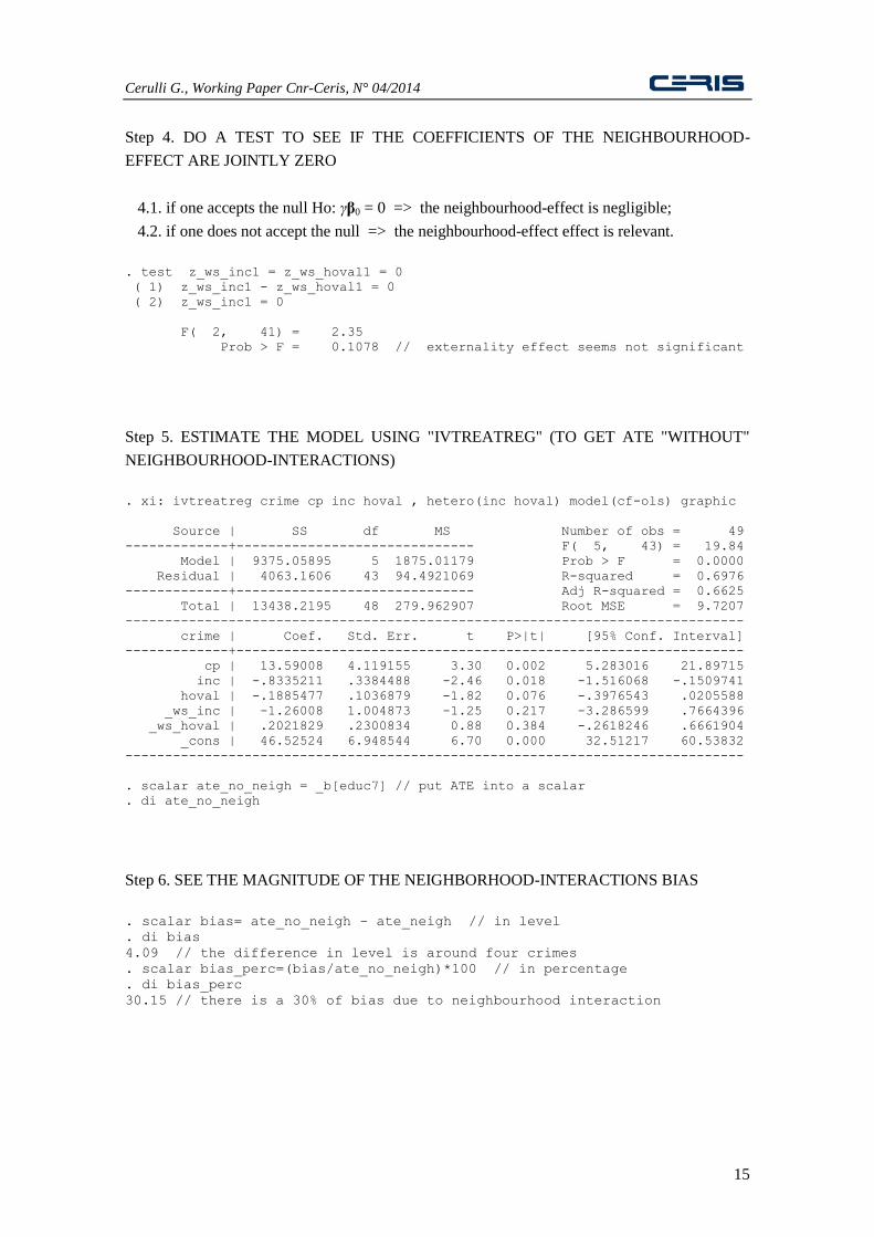
Step 4. DO A TEST TO SEE IF THE COEFFICIENTS OF THE NEIGHBOURHOOD-

EFFECT ARE JOINTLY ZERO

4.1. if one accepts the null Ho: γβ0 = 0 => the neighbourhood-effect is negligible;

4.2. if one does not accept the null => the neighbourhood-effect effect is relevant.

. test z_ws_inc1 = z_ws_hoval1 = 0

( 1) z_ws_inc1 - z_ws_hoval1 = 0

( 2) z_ws_inc1 = 0

F( 2, 41) = 2.35

Prob > F = 0.1078 // externality effect seems not significant

Step 5. ESTIMATE THE MODEL USING "IVTREATREG" (TO GET ATE "WITHOUT"

NEIGHBOURHOOD-INTERACTIONS)

. xi: ivtreatreg crime cp inc hoval , hetero(inc hoval) model(cf-ols) graphic


-------------+------------------------------ F( 5, 43) = 19.84

Model | 9375.05895 5 1875.01179 Prob > F = 0.0000


-------------+------------------------------ Adj R-squared = 0.6625

Total | 13438.2195 48 279.962907 Root MSE = 9.7207

------------------------------------------------------------------------------

crime | Coef. Std. Err. t P>|t| [95% Conf. Interval]

-------------+----------------------------------------------------------------

cp | 13.59008 4.119155 3.30 0.002 5.283016 21.89715

inc | -.8335211 .3384488 -2.46 0.018 -1.516068 -.1509741

hoval | -.1885477 .1036879 -1.82 0.076 -.3976543 .0205588

_ws_inc | -1.26008 1.004873 -1.25 0.217 -3.286599 .7664396

_ws_hoval | .2021829 .2300834 0.88 0.384 -.2618246 .6661904

_cons | 46.52524 6.948544 6.70 0.000 32.51217 60.53832

------------------------------------------------------------------------------

. scalar ate_no_neigh = _b[educ7] // put ATE into a scalar

. di ate_no_neigh

Step 6. SEE THE MAGNITUDE OF THE NEIGHBORHOOD-INTERACTIONS BIAS

. scalar bias= ate_no_neigh - ate_neigh // in level

. di bias

4.09 // the difference in level is around four crimes

. scalar bias_perc=(bias/ate_no_neigh)*100 // in percentage

. di bias_perc

30.15 // there is a 30% of bias due to neighbourhood interaction


16

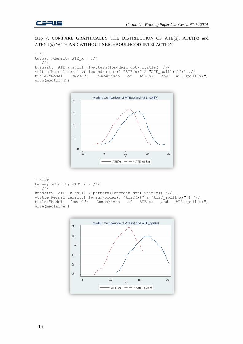
Step 7. COMPARE GRAPHICALLY THE DISTRIBUTION OF ATE(x), ATET(x) and

ATENT(x) WITH AND WITHOUT NEIGHBOURHOOD-INTERACTION * ATE

twoway kdensity ATE_x , ///

|| ///

kdensity _ATE_x_spill ,lpattern(longdash_dot) xtitle() ///

ytitle(Kernel density) legend(order(1 "ATE(x)" 2 "ATE_spill(x)")) ///

title("Model `model': Comparison of ATE(x) and ATE_spill(x)",

size(medlarge))

* ATET

twoway kdensity ATET_x , ///

|| ///

kdensity _ATET_x_spill ,lpattern(longdash_dot) xtitle() ///

ytitle(Kernel density) legend(order(1 "ATET(x)" 2 "ATET_spill(x)")) ///


size(medlarge))

.04

.06

.08

.1.1

2.1

4

Ke

rne

l de

nsity

5 10 15 20x

ATET(x) ATET_spill(x)

Model : Comparison of ATE(x) and ATE_spill(x)

0

.02

.04

.06

.08

Ke

rne

l de

nsity

-10 0 10 20 30x

ATE(x) ATE_spill(x)



17

* ATENT

twoway kdensity ATENT_x , ///

|| ///

kdensity _ATENT_x_spill ,lpattern(longdash_dot) xtitle() ///

ytitle(Kernel density) legend(order(1 "ATENT(x)" 2 "ATENT_spill(x)")) ///


size(medlarge))

As a conclusion, we can state that if the

analyst does not consider “neighbourhood

effects” she will “over-estimate” the actual

effect of housing location on crime of around

a 30%. However, the test seems to show that

the neighbourhood effect is not relevant, as

the coefficients of the neighbourhood

component of regression (14) are not jointly

significant.

5.2 Example 2: the effect of education

on fertility

As a second application, we consider the

dataset “FERTIL2_200.DTA” accompanying

the manual “Introductory Econometrics: A

Modern Approach” by Wooldridge (2000),

where we consider only N=200 (out of 4,361)

randomly drawn women in childbearing age

in Botswana. The aim of this application is

that of evaluating the impact of education on

fertility, i.e. the causal effect of the variable

“educ7” - taking value 1 if a woman has more

than or exactly seven years of education and 0

otherwise - on the number of family children

(the variable “children”). Several conditioning

(or confounding) observable factors are

included in the dataset, such as the age of the

woman (“age”), whether or not the family

owns a TV (“tv”), whether or not the woman

lives in a city (“urban”), and so forth. We are

particularly interested in detecting the effect

of education on fertility in such a setting, by

taking into account possible peer-interactions

among women. In particular, our research

presumption is that: “in choosing their

‘desired’ number of children, less educated

women (the untreated ones) are not only

affected by their own (idiosyncratic)

characteristics (the x), but also by the number

of children chosen by more educated women”.

The conjecture behind this statement is that

less educated women might want to be as like

as possible to more educated ones as a way to

avoid some form of social stigma.

0

.02

.04

.06

.08

Ke

rne

l de

nsity

-10 0 10 20 30x

ATENT(x) ATENT_spill(x)



18

Step 0. INPUT DATA FOR THE REGRESSION MODEL

y: children

w: educ7

x: age agesq evermarr electric tv

Matrix Ω: dist

Step 1. LOAD THE STATA ROUTINE "NTREATREG" AND THE DATASET

. ssc install ntreatreg

. use "FERTIL2_200.DTA"

Step 2. PROVIDE THE MATRIX "OMEGA" (HERE WE CALL IT "dist")

. matrix dissimilarity dist = age agesq urban electric tv , corr // we use

correlation weights

. matewmf dist dist_abs, f(abs) // take the absolute values of the OMEGA

Step 3. ESTIMATE THE MODEL USING "NTREATREG" TO GET THE “ATE” WITH

NEIGHBORHOOD-INTERACTIONS

. set more off

. xi: ntreatreg children educ7 age agesq evermarr electric tv , ///

hetero(age agesq evermarr) spill(dist_abs) graphic


-------------+------------------------------ F( 12, 187) = 17.62

Model | 493.24433 12 41.1036942 Prob > F = 0.0000


-------------+------------------------------ Adj R-squared = 0.5005

Total | 929.58 199 4.67125628 Root MSE = 1.5275

--------------------------------------------------------------------------------

children | Coef. Std. Err. t P>|t| [95% Conf. Interval]

---------------+----------------------------------------------------------------

educ7 | -.3869939 .2405745 -1.61 0.109 -.8615826 .0875948

age | -.004031 1.109614 -0.00 0.997 -2.193002 2.18494

agesq | -.0037554 .0098361 -0.38 0.703 -.0231595 .0156486

evermarr | .7954806 .3436893 2.31 0.022 .117474 1.473487

electric | -1.173366 .5034456 -2.33 0.021 -2.166529 -.1802034

tv | .358726 .6334492 0.57 0.572 -.8908988 1.608351

_ws_age | -.1171632 .1797361 -0.65 0.515 -.4717342 .2374077

_ws_agesq | .0013009 .0029585 0.44 0.661 -.0045354 .0071372

_ws_evermarr | .0212155 .5385761 0.04 0.969 -1.04125 1.083681

z_ws_age1 | 5041.887 8015.575 0.63 0.530 -10770.69 20854.46

z_ws_agesq1 | -151.9131 230.3377 -0.66 0.510 -606.3075 302.4812

z_ws_evermarr1 | 93992.24 130909.8 0.72 0.474 -164257.6 352242.1

_cons | 14492.64 11104.22 1.31 0.193 -7412.988 36398.27

--------------------------------------------------------------------------------

. scalar ate_neigh = _b[educ7] // put ATE into a scalar

. di ate_neigh

-.3869939

. rename ATE_x _ATE_x_spill // rename ATE_x as _ATE_x_spill

. rename ATET_x _ATET_x_spill

. rename ATENT_x _ATENT_x_spill


19

Step 4. DO A TEST TO SEE IF THE COEFFICIENTS OF THE NEIGHBOURHOOD-

EFFECT ARE JOINTLY ZERO

4.1. if one accepts the null Ho: γβ0 = 0 => the neighbourhood-effect is negligible;

4.2. if one does not accept the null => the neighbourhood-effect effect is relevant.

. test z_ws_age1 = z_ws_agesq1 = z_ws_evermarr1 = 0

( 1) z_ws_age1 - z_ws_agesq1 = 0

( 2) z_ws_age1 - z_ws_evermarr1 = 0

( 3) z_ws_age1 = 0

F( 3, 187) = 2.49

Prob > F = 0.0619 // social interaction significant at 6%

Step 5. ESTIMATE THE MODEL USING "IVTREATREG" (TO GET ATE "WITHOUT"

NEIGHBOURHOOD-INTERACTIONS)

. xi: ivtreatreg children educ7 age agesq evermarr electric tv , ///

hetero(age agesq evermarr) model(cf-ols) graphic


-------------+------------------------------ F( 9, 190) = 22.14

Model | 475.829139 9 52.8699044 Prob > F = 0.0000


-------------+------------------------------ Adj R-squared = 0.4888

Total | 929.58 199 4.67125628 Root MSE = 1.5454

------------------------------------------------------------------------------

children | Coef. Std. Err. t P>|t| [95% Conf. Interval]

-------------+----------------------------------------------------------------

educ7 | -.4581193 .2417352 -1.90 0.060 -.9349488 .0187101

age | .4703103 .1252132 3.76 0.000 .2233237 .7172968

agesq | -.0053527 .0019811 -2.70 0.008 -.0092605 -.001445

evermarr | .7601864 .3439046 2.21 0.028 .0818249 1.438548

electric | -.8397923 .4060984 -2.07 0.040 -1.640833 -.0387517

tv | .1892151 .4754544 0.40 0.691 -.7486321 1.127062

_ws_age | -.1412403 .1788508 -0.79 0.431 -.4940286 .211548

_ws_agesq | .0018331 .0029337 0.62 0.533 -.0039537 .0076199

_ws_evermarr | .0667193 .543741 0.12 0.902 -1.005825 1.139264

_cons | -6.409861 1.83986 -3.48 0.001 -10.03904 -2.780685

------------------------------------------------------------------------------

. scalar ate_no_neigh = _b[educ7] // put ATE into a scalar

. di ate_no_neigh

-.45811935

Step 6. SEE THE MAGNITUDE OF THE NEIGHBORHOOD-INTERACTIONS BIAS

. scalar bias= ate_no_neigh - ate_neigh // in level

. di bias

-.07112545

. scalar bias_perc=(bias/ate_no_neigh)*100 // in percentage

. di bias_perc

15.525528 // there is a 15% of bias due to social interaction


20

Step 7. COMPARE GRAPHICALLY THE DISTRIBUTION OF ATE(x), ATET(x) and

ATENT(x) WITH AND WITHOUT NEIGHBOURHOOD-INTERACTION

* ATE

twoway kdensity ATE_x , ///

|| ///

kdensity _ATE_x_spill ,lpattern(longdash_dot) xtitle() ///

ytitle(Kernel density) legend(order(1 "ATE(x)" 2 "ATE_spill(x)")) ///


size(medlarge))

* ATET

twoway kdensity ATET_x , ///

|| ///

kdensity _ATET_x_spill ,lpattern(longdash_dot) xtitle() ///

ytitle(Kernel density) legend(order(1 "ATET(x)" 2 "ATET_spill(x)")) ///

title("Model `model': Comparison of ATE(x) and ATE_spill(x)", size(medlarge))

0.5

11

.5

Ke

rne

l de

nsity

-1 -.5 0 .5x

ATE(x) ATE_spill(x)


.4.6

.81

1.2

Ke

rne

l de

nsity

-.8 -.6 -.4 -.2 0 .2x

ATET(x) ATET_spill(x)



21

* ATENT

twoway kdensity ATENT_x , ///

|| ///

kdensity _ATENT_x_spill ,lpattern(longdash_dot) xtitle() ///

ytitle(Kernel density) legend(order(1 "ATENT(x)" 2 "ATENT_spill(x)")) ///

title("Model `model': Comparison of ATE(x) and ATE_spill(x)", size(medlarge))

As a conclusion, we can state that if the

analyst does not consider neighbourhood

effects, she will “over-estimate” the actual

effect of education on fertility of around a

15%. Furthermore, the test shows that the

neighbourhood effect is relevant, as the

coefficients of the neighbourhood component

of regression (14) are jointly significant.

How can we interpret such a result? A

possible argument can be that there is a peer-

effect in choosing how many children to have

by women. Indeed, as said before, the

“desired” number of children for a woman

does not depend only on her individual

determinants (“age”, for instance), but also on

“what my friends do”. In our sample, the

existence of such a “social interaction”

reduces the “effect of education on fertility”

(from 0.45 to 0.38 on absolute values), by

showing that fertility behaviour of more

educated women (generally unconditionally

less fertile) produce a spillover on less

educated ones, by pushing them to reduce the

number of children to have. This might be a

typical “imitative behaviour” on the part of

less educated women striving to be as much

similar as possible to more educated ones.

Therefore, “education” has an effect on

“fertility”, not only because schooling can

delay the time to have a child, but also

because education “triggers” imitative peer-

effects.

6. CONCLUSION

This paper has presented a possible solution

to incorporate externality (or neighbourhood)

effects within the traditional Rubin’s potential

outcome model under conditional mean

independence. As such, it generalizes the

traditional parametric models of program

evaluation when SUTVA is relaxed. As by-

0.5

11

.52

2.5

Ke

rne

l de

nsity

-1 -.5 0 .5x

ATENT(x) ATENT_spill(x)



22

product, this work has also put forward

ntreatreg, a Stata routine for estimating

Average Treatments Effects (ATEs) when

social interactions are present.

The two instructional applications to the

causal effect of housing location on crime,

and of education on fertility, seem to show

that such approach can change significantly

usual no-interaction results in those fields of

social and economic contexts where

externalities due to units’ interaction may be

pervasive.

Of course, this approach presents also some

limitations, and in what follows we list some

of its potential developments. Indeed, the

model might be improved by:

allowing also for treated units to be

affected by other treated units’ outcome;

extending the model to “multiple” or

“continuous” treatment, when treatment

may be multi-valued or fractional for

instance, by still holding CMI;

identifying ATEs with neighbourhood

interactions when w may be endogenous

(i.e., relaxing CMI) by implementing

GMM-IV estimation;

trying to go beyond the potential

outcomes’ parametric form, by relying on

a semi-parametric specification;

providing Monte Carlo studies to check

to which extent are model’s results robust

under different specification-errors in the

weighting matrix Ω.

Finally, an interesting issue deserving

further inquiry regards the assumption of

exogeneity concerning the weighting matrix

Ω. Indeed, a challenging question might be:

what happens if individuals strategically

modify their weighting weights to better profit

of others’ treatment outcome? It is clear that

weights do become endogenous, thus yielding

severe identification problems for previous

causal effects. Future studies should tackle

situations in which this possibility may occur.


23

REFERENCES

Anselin, L. (1988), Spatial Econometrics:

Methods and Models. Boston: Kluwer

Academic Publishers.

Aronow, P.M. and Cyrus, Samii C. (2013),

Estimating average causal effects under

interference between units. Unpublished

manuscript, May 28.

Cox, D.R. (1958), Planning of Experiments,

New York, Wiley.

Holland, P.W. (1986), Statistics and causal

inference, Journal of the American

Statistical Association, 81, 396, 945–960.

Hudgens, M. G. and Halloran, M.E. (2008),

Toward causal inference with interference,

Journal of the American Statistical

Association, 103, 482, 832–842.

Imbens, W.G. and Angrist, J.D. (1994),

Identification and estimation of local

average treatment effects, Econometrica, 62,

2, 467–475.

Manski, C.F.(1993), Identification of

endogenous social effects: The reflection

problem, The Review of Economic Studies,

60, 3, 531–542.

Manski, C.F. (2013), Identification of

treatment response with social interactions,

The Econometrics Journal, 16, 1, S1–S23.

Robins, J. M., Hernan, M.A. and Brumback,

B. (2000), Marginal structural models and

causal inference in epidemiology,

Epidemiology, 11, 5, 550–560.

Rosenbaum, P.R. (2007). Interference

between units in randomized experiments.


Association, 102, 477, 191–200.

Rubin, D.B. (1974), Estimating Causal Effects

of Treatments in Randomized and

Nonrandomized Studies, Journal of

Educational Psychology, 66, 5, 688–701.

Rubin, D.B. (1977), Assignment to treatment

group on the basis of a covariate, Journal of

Educational Statistics, 2, 1, 1–26.

Rubin, D.B. (1978), Bayesian inference for

causal effects: The role of randomization,

Annals of Statistics, 6, 1, 34–58.

Sobel, M.E. (2006), What do randomized

studies of housing mobility demonstrate?:

Causal inference in the face of interference,


Association, 101, 476, 1398–1407.

Tchetgen-Tchetgen, E. J. and VanderWeele,

T.J. (2010), On causal inference in the

presence of interference, Statistical Methods

in Medical Research, 21, 1, 55-75.

Wooldridge, J.M. (1997), On two stage least

squares estimation of the average treatment

effect in a random coefficient model,

Economics Letters, 56, 2, 129-133.

Wooldridge, J.M. (2010), Econometric

Analysis of Cross Section and Panel Data,

Cambridge, MA: The MIT Press.


24

APPENDIX A

In this appendix, we show how to obtain the formulas of ATE and ATE(x) set out in (12) and

(13). Then, we show how regression (14) can be obtained and, finally, we prove that

Assumption 1 is sufficient for consistently estimating the parameters of regression (14) by OLS.

A1. Formula of ATE with neighbourhood interactions.

Given assumptions 2 and 3, and the implied equations in (7), we get that:

1 1

1 1

1 0 1 1 1 0 0 1 1 1 0

1 1

1 1 1 0 0 1 1 1 0

1 1

1 1 1 0

ATE = E( ) E

E

E

N N

i i i i i ij j ij j i

j j

N N

i i i ij j ij j i

j j

i i

y y e e e

e e e

e

x β x β x β

x β x β x β

x β1 1

1 1

1 1

0 1 1 1 0

1 1

1 1 0 1 0 1 1 1 0

1 1

1 0 1 0 1 1 1 0

1 1

E

=E (1 ) ( )

N N

i ij j ij j i

j j

N N

i i ij j ij j i i

j j

N N

i ij j ij j i i

j j

e e

e e e

e e e

x β x β

x β x β x β

x β β x β

1 1

1 1

1 0 1 1 1 0

1 1

1 1

1 1

E (1 )

E

N N

i ij j ij j i i

j j

N N

i ij j i i ij j

j j

e e e

e

x δ x β

x δ x β x δ x β

where 1 0 = (1 ) , = E( )j jx x and 1 0 δ β β .

A2. Formula of ATE(xi) with neighbourhood interactions.

Given assumptions 2 and 3, and the result in A1, we get:

1 1

1 1 1 1

1 0 1 1

1 1

1 1 1 1

1 1 1 1

ATE( ) = E( | ) E |

[ ] ( ) ( )

N N

i i i i i ij j i i i ij j

j j

N N N N

ij ij ij i ij j

j j j j

y y e

x x x δ x β x x δ x β

xδ xδ x β x β xδ x β x x δ x x β

1

1

1

ATE+( ) ( )N

i ij j

j

x x δ x x β


25

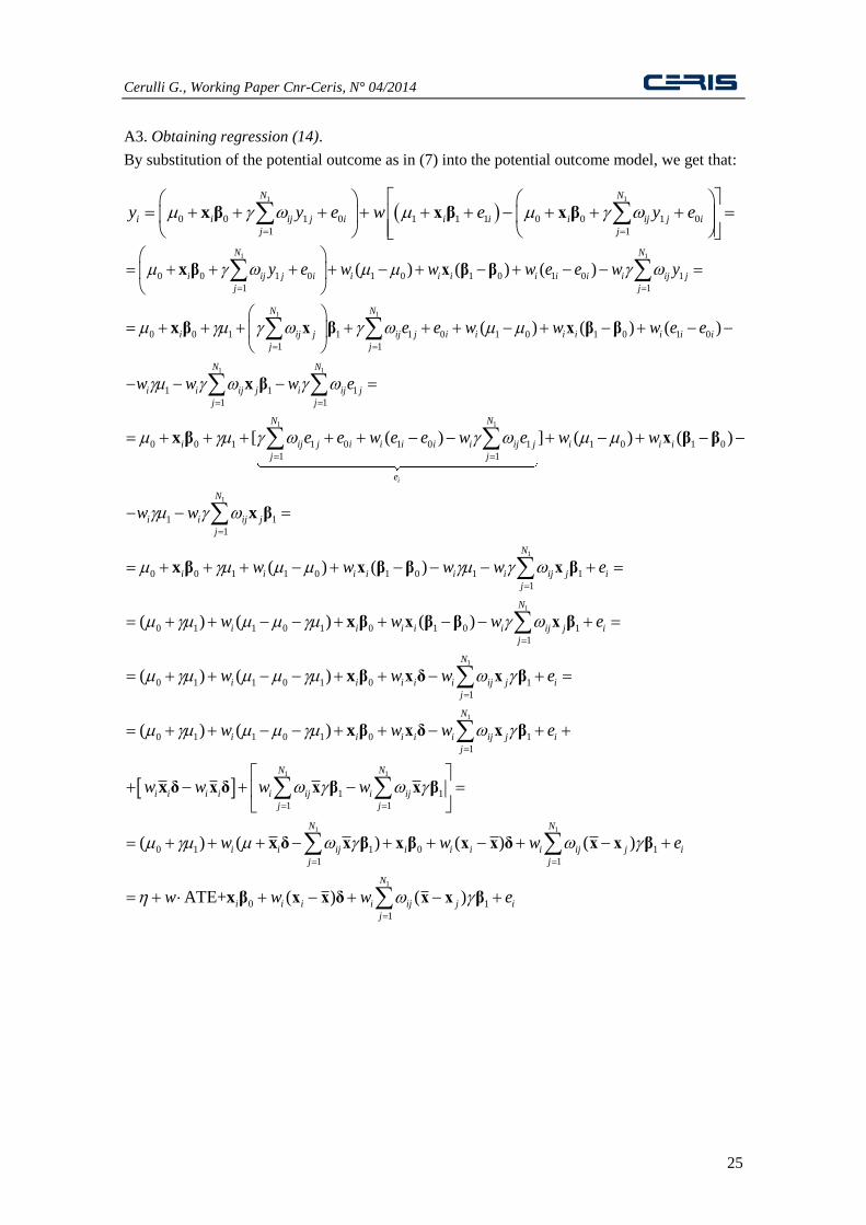
A3. Obtaining regression (14).

By substitution of the potential outcome as in (7) into the potential outcome model, we get that:

1 1

0 0 1 0 1 1 1 0 0 1 0

1 1

N N

i i ij j i i i i ij j i

j j

y y e w e y e

x β x β x β

1 1

1 1

1

0 0 1 0 1 0 1 0 1 0 1

1 1

0 0 1 1 1 0 1 0 1 0 1 0

1 1

1 1

1

( ) ( ) ( )

( ) ( ) ( )

N N

i ij j i i i i i i i i ij j

j j

N N

i ij j ij j i i i i i i i

j j

N

i i ij j i ij

j j

y e w w w e e w y

e e w w w e e

w w w

x β x β β

x β x β x β β

x β1

1

1

N

je

1 1

1

1

0 0 1 1 0 1 0 1 1 0 1 0

1 1

1 1

1

0 0 1 1 0 1 0 1 1

1

0 1

[ ( ) ] ( ) ( )

( ) ( )

( ) (

i

N N

i ij j i i i i i ij j i i i

j j

e

N

i i ij j

j

N

i i i i i i ij j i

j

i

e e w e e w e w w

w w

w w w w e

w

x β x β β

x β

x β x β β x β

1

1

1

1 1

1 0 1 0 1 0 1

1

0 1 1 0 1 0 1

1

0 1 1 0 1 0 1

1

1

1 1

) ( )

( ) ( )

( ) ( )

N

i i i i ij j i

j

N

i i i i i ij j i

j

N

i i i i i ij j i

j

N N

i i i i i ij i ij

j j

w w e

w w w e

w w w e

w w w w

x β x β β x β

x β x δ x β

x β x δ x β

x δ x δ x β x

1 1

1

1

0 1 1 0 1

1 1

0 1

1

( ) ( ) ( ) ( )

ATE+ ( ) ( )

N N

i i ij i i i i ij j i

j j

N

i i i i ij j i

j

w w w e

w w w e

β

x δ x β x β x x δ x x β

x β x x δ x x β


26

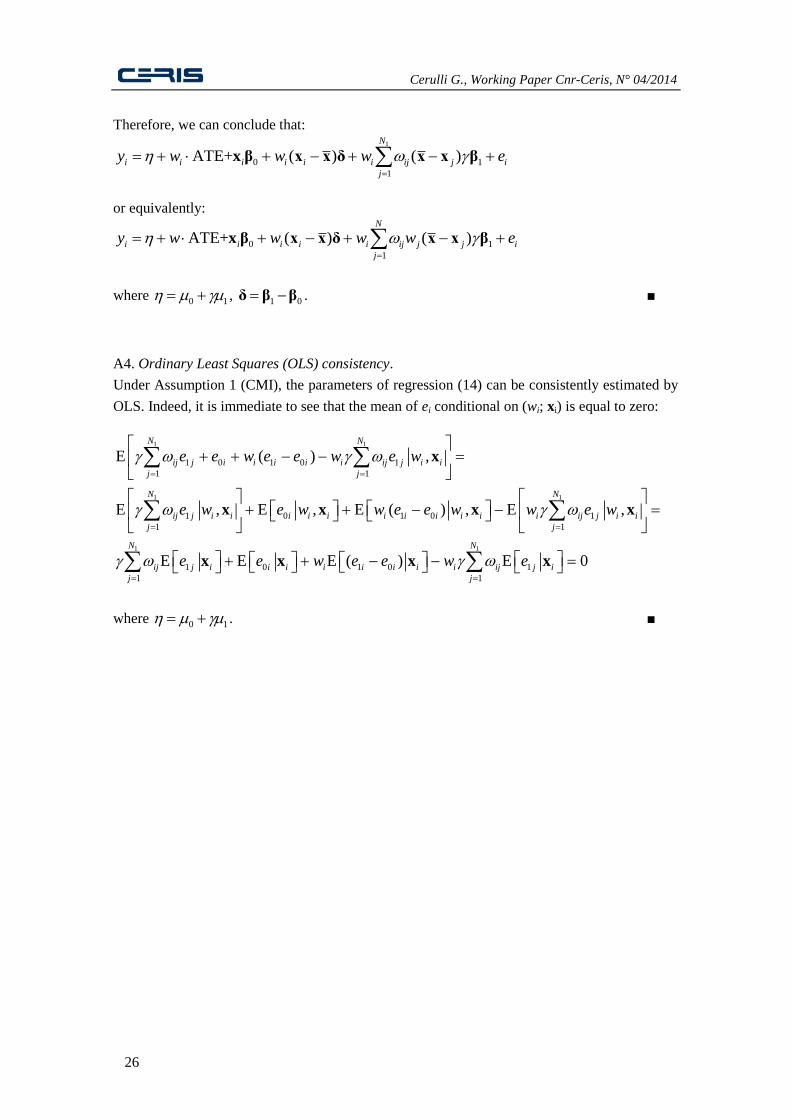
Therefore, we can conclude that:

1

0 1

1

ATE+ ( ) ( )N

i i i i i i ij j i

j

y w w w e

x β x x δ x x β

or equivalently:

0 1

1

ATE+ ( ) ( )

N

i i i i i ij j j i

j

y w w w w ex β x x δ x x β

where 0 1 , 1 0 δ β β .

A4. Ordinary Least Squares (OLS) consistency.

Under Assumption 1 (CMI), the parameters of regression (14) can be consistently estimated by

OLS. Indeed, it is immediate to see that the mean of ei conditional on (wi; xi) is equal to zero:

1 1

1 1

1

1 0 1 0 1

1 1

1 0 1 0 1

1 1

1 0 1 0

1

E ( ) ,

E , E , E ( ) , E ,

E E E ( )

N N

ij j i i i i i ij j i i

j j

N N

ij j i i i i i i i i i i i ij j i i

j j

N

ij j i i i i i i i

j

e e w e e w e w

e w e w w e e w w e w

e e w e e w

x

x x x x

x x x1

1

1

E 0N

i ij j i

j

e

x

where 0 1 .

Working Paper Cnr-Ceris

ISSN (print): 1591-0709 ISSN (on line): 2036-8216

Download

www.ceris.cnr.it/index.php?option=com_content&task=section&id=4&Itemid=64

Hard copies are available on request,

please, write to:

Cnr-Ceris

Via Real Collegio, n. 30

10024 Moncalieri (Torino), Italy

Tel. +39 011 6824.911 Fax +39 011 6824.966

[email protected] www.ceris.cnr.it

Copyright © 2014 by Cnr–Ceris

All rights reserved. Parts of this paper may be reproduced with the permission

of the author(s) and quoting the source.


cover new impa ceris 2010 - Stata · cover new impa ceris 2010 26-01-2010 7:36 Pagina 1. l\rWorking...

Documents

Transcript of cover new impa ceris 2010 - Stata · cover new impa ceris 2010 26-01-2010 7:36 Pagina 1. l\rWorking...