Bilinear Relationship Model Development of the Fathead Minnow

JOURNAL OF MATHEMATICAL PSYCHOLOGY 28, 1-42 (1984)
Conjoint Design and Analysis of the Bilinear Model: An Application to Judgments of Risk
CLYDE H. COOMBS AND PAUL E. LEHNER*
The University of Michigan
Conjoint measurement tests which are applicable to a (2 X 2) x (2 X 2) experimental design for the study of the general bilinear model are developed. The tests permit detecting the cause of each failure of the data to satisfy the model, and of measuring the tradeoffs between variables when the model is satisfied. All tests and analyses are illustrated with an application of the model to the assessment of the riskiness of gambles. The method is compared with the use of duplex gambles and other compound and contingent compositions in terms of their appropriate roles in the study of the decision process.
Table of Contents. Introduction. Subjects. Procedures. Analysis and Results. Assessing error in the data. Additivity and independence of good and bad components. Associated variables. Unassociated variables. Discussion. Summary.
In a previous paper (Coombs & Lehner, 1981) it was found that symmetric changes in good and bad outcomes are not equal in their effects on judged risk. As a consequence, moments of distributions are unacceptable as variables for measuring risk. Variance, for example, is invariant under translation of a distribution and if the distribution is skewed the riskiness of a gamble can be expected to reveal triple interactions, and so cannot be captured in a simple polynomial as defined in Krantz, Lute, Suppes, & Tversky (1971).
An obvious prospect, then, is a model which separates the effects of good and bad outcomes, and here we propose testing a theory which does that. The formal structure of the theory is that of the bilinear model (Kruskal, 1978) and we use an experimental design which makes possible a conjoint measurement analysis of this model not previously feasible.
A bilinear model is one in which the independent variables can be partitioned into two subsets such that if either subset is held constant, the dependent variable is a linear function of the variables in the other subset. Common examples include models
This research was supported in part by NSF Research Grants BNS 78-09191 and BNS 81-20299. We are indebted to William Goldstein, David Krantz, Keith Levi, and Amos Tversky for discussions in the course of developing the design and analysis and to James Shanteau and Paul Slavic for valuable critical reactions to an earlier draft.
* Present address: Par Technology Corp., 7926 Jones Branch Drive, Suite 170, McLean, Virginia 22102.
0022.2496184 $3.00 Copyright 0 1984 by Academic Press, Inc.
All rights of reproduction in any form reserved.

2 COOMBS AND LEHNER
of decision making and applications of multiattribute utility theory. In these instances, outcomes constitute one set of variables and probabilities or weights the other set. Familiar examples are models of risky decision making as found in Edwards (1955), Huang’s theory of expected risk (1975), Kahneman and Tversky’s prospect theory (1979), and a vast number of instances in which the model is used in assessment, evaluation, prediction, and control; see, for example, Huber (1974) and Feather (1982).
The model is perhaps the most common in behavioral science. A very incomplete list of examples from psychology alone includes Anderson’s (1974) models of infor- mation integration; Atkinson’s (1957) motivational theory modeled in terms of probabilities and incentives; Berliner’s (1974) program for backgammon in which the same board position has a different weighting function for each alternative strategy which are then summed up and maximized; Edwards (1962) weighted subjectively expected utility model and all special cases of it in which the worth of a gamble is an additive function of the worth of the outcomes weighted by some function of their probabilities; Fishbein’s theory (Fishbein & Ajzin, 1975) of the relationship between beliefs, attitudes, and behavior; Helson’s (1964) model of adaptation level in terms of focal stimuli, background stimuli, and residual stimuli, Osgood’s (1956) semantic differential for the measurement of affective meaning as a function of evaluation, potency, and activity; Rosenberg’s (1960) structural theory of attitude dynamics in which attitude change is viewed as a function of the discrepancy between the affective and the cognitive components of the attitude; Slate and Atkins’ (1977) chess playing program which evaluates a board position by a linear weighting of features of the board; Triandis’ (1972) conception of subjective culture in terms of norms, ideals, abilities, values, habits, expectations, costs, rewards, etc.; and Zajonc’s (1954) theory of attitude as a function of valence and prominence.
These theories were deliberately chosen to illustrate a range over a wide variety of subject matters, but as formal models they are closely related, and the methodology developed here for testing the bilinear model is applicable in principle to all.
The bilinear model has, of course, been given a lot of attention already. The most closely related development, perhaps, is the extension by Anderson and Shanteau (1970) of functional measurement theory to the bilinear model. What is unique to the present paper is the extension of conjoint measurement theory using only ordinal properties of the data which is made possible by utilizing a particular experimental design.
An application to illustrate this development is in the context of a model for the measurement of risk, in which a risk ordering is the dependent variable. Our bilinear model for the assessment of risk asserts that risk is an additive combination of the effect of the bad aspects and the effect of the good aspects and that these two effects are each a consequence of their respective outcomes and associated probabilities.
In the simple case of lotteries with monetary outcomes, one positive, and one negative (and one zero to permit some freedom in the manipulation of probabilities), the model takes the following form. If we let w, 1, and 0 represent good, bad, and zero outcomes, respectively, with p and q the probabilities associated with the good
ANALYSIS OF THE BILINEAR MODEL 3
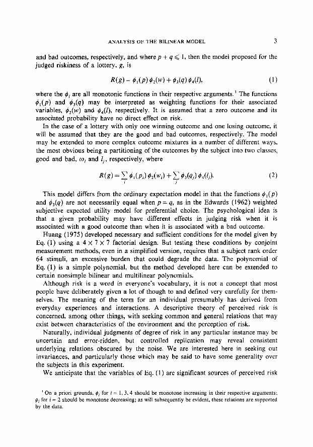
and bad outcomes, respectively, and wherep + q < 1, then the model proposed for the judged riskiness of a lottery, g, is
R(g) = #l(P) h(w) + h(4) 44(9, (1)
where the $i are all monotonic functions in their respective arguments.’ The functions $l(p) and 03(q) may be interpreted as weighting functions for their associated variables, &(w) and #4(1), respectively. It is assumed that a zero outcome and its associated probability have no direct effect on risk.
In the case of a lottery with only one winning outcome and one losing outcome, it will be assumed that they are the good and bad outcomes, respectively. The model may be extended to more complex outcome mixtures in a number of different ways, the most obvious being a partitioning of the outcomes by the subject into two classes, good and bad, wi and lj, respectively, where
This model differs from the ordinary expectation model in that the functions 4,(p) and 4,(q) are not necessarily equal when p = q, as in the Edwards (1962) weighted subjective expected utility model for preferential choice. The psychological idea is that a given probability may have different effects in judging risk when it is associated with a good outcome than when it is associated with a bad outcome.
Huang (1975) developed necessary and sufficient conditions for the model given by Eq. (1) using a 4 x 7 x 7 factorial design. But testing these conditions by conjoint measurement methods, even in a simplified version, requires that a subject rank order 64 stimuli, an excessive burden that could degrade the data. The polynomial of Eq. (1) is a simple polynomial, but the method developed here can be extended to certain nonsimple bilinear and multilinear polynomials.
Although risk is a word in everyone’s vocabulary, it is not a concept that most people have deliberately given a lot of though to and defined very carefully for them- selves. The meaning of the term for an individual presumably has derived from everyday experiences and interactions. A descriptive theory of perceived risk is concerned, among other things, with seeking common and general relations that may exist between characteristics of the environment and the perception of risk.
Naturally, individual judgments of degree of risk in any particular instance may be uncertain and error-ridden, but controlled replication may reveal consistent underlying relations obscured by the noise. We are interested here in seeking out invariances, and particularly those which may be said to have some generality over the subjects in this experiment.
We anticipate that the variables of Eq. (1) are significant sources of perceived risk
’ On a priori grounds, $I for i = 1,3,4 should be monotone increasing in their respective arguments; (i for i = 2 should be monotone decreasing; as will subsequently be evident, these relations are supported by the data.
4 COOMBS AND LEHNER
and that certain monotonic relations are to be anticipated. But more subtle than these are invariances in the tradeoffs among these variables, and so questions arise as to what may be said about such tradeoffs that has some commonality or generality. We have used a particular experimental design and developed some new analytical methods which sharpen these questions and permit partial answers.
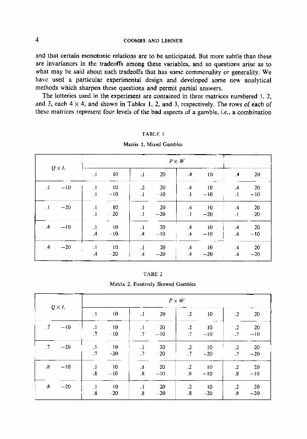
The lotteries used in the experiment are contained in three matrices numbered 1, 2, and 3, each 4 X 4, and shown in Tables 1, 2, and 3, respectively. The rows of each of these matrices represent four levels of the bad aspects of a gamble, i.e., a combination
TABLE I
Matrix 1, Mixed Gambles
PXW
QxL .l 10 .l 20 .4 10 .4 20
.l -10 .l 10 .2 20 A 10 .4 20 .l -10 .l -10 .I -10 .I -10
.I -20 .I 10 .l 20 .4 10 .4 20
.l -20 .l -20 .l -20 .l -20
.4 -10 .I 10 .l 20 .4 10 .4 20
.4 -10 .4 -10 j .4 -10 .4 -10 I
.4 -20 .l 10 I .l 20 i .4 10 .4 20
.4 -20 .4 -20 ! .4 -20 .4 -20
TABE 2
Matrix 2, Positively Skewed Gambles
PX w
QxL .l 10 .I 20 .2 10 .2 20
.I -10 .l 10 .I 20 .2 10 .2 20
.7 -10 .I -10 .I -10 .l -10
’ .7 -20 .l 10 .I 20 .2 10 .2 20
.l -20 .7 -20 .7 -20 .7 -20
.8 -10 .l 10 .I 20 i .2 10 .2 20
.8 -10 .8 -10 .8 -10 .8 -10
.8 -20 .l 10 .l 20 .2 10 .2 20 .8 -20 .8 -20 .8 -20 .8 -20

ANALYSIS OF THE BILINEAR MODEL 5
TABLE 3
Matrix 3, Negatively Skewed Gambles
PXW QxL
.I 10 .I 20 .8 10 .8 20
.l -10 .I 10 .I 20 .8 10 .8 20
.l -10 .l -10 .l -10 .l -10
.I -20 .7 10 .7 20 .8 10 .8 20
.l -20 .l -20 .l -20 .l -20
.2 -10 .I 10 .I 20 .8 10 .8 20
.2 -10 .2 -10 .2 -10 .2 -10
.2 -20 .I 10 .I 20 .8 10 .8 20
.2 -20 .2 -20 .2 -20 .2 -20
of a probablity of losing, q, and an amount to lose, 1. The columns of each of these matrices represent four levels of the good aspects, a combination of a probablity of winning, p, and an amount to win, W. In these three matrices, p and q were varied independently, leaving a residual probability, 1 - p - q, as the probability of the zero outcome. The zero outcome and its probability are not shown in the three tables for clarity of presentation.
The levels of the experimentally independent variables, Q, L, P, and W, were chosen so that matrix 1 contains a mixture of symmetric and asymmetric gambles, those in matrix 2 are all positively skewed, and those in matrix 3 are all negatively skewed. The expected values of the gambles are all negative in matrix 2, are all positive in matrix 3, and they are mixed in matrix 1. The purpose of this, of course, was to increase the generality of the results.
The design of the stimulus matrices is (2 x 2) x (2 x 2), which is very rich in its potential for controlled piecemeal analysis. Because of the intimate relation between the design and the development of the new conjoint measurement tests, further discussion of the design is postponed to the appropriate sections of the analysis.
Each stimulus was displayed on a wheel of fortune on a card 2 x 24 in. The winning and losing amounts were displayed numerically, while the probabilities were displayed by pie sections on the wheel of fortune. The cards for each matrix were assembled into separate stacks of 16 cards; each stack corresponded to one of the matrices.
Subjects
The subjects were 44 student volunteers from the University of Michigan paid subject pool.

6 COOMBSANDLEHNER
Procedure
Each subject participated in three experimental sessions on three separate, not necessarily consecutive, days. Data were collected in each experimental session on seven stimulus matrices, the three shown in Table 1, 2, and 3, and four others, also 4 x 4 which contained the gambles used for the previous paper referred to above (Coombs & Lehner, 1981). On each day subjects were asked to rank order each of the stacks of gambles with respect to risk by using the method of accumulation (Coombs & Bowen, 1971). The order of the gambles in each stack and the order in which the stacks were presented to each subject were randomized. Each subject was left to define risk in his/her own terms, our interest being in the descriptive theory of perceived risk as a function of final outcomes and probabilities.
ANALYSIS AND RESULTS
Assessing Error in the Data
Implicit in the search for invariances embedded in noise is an error theory. There is, as yet, no adequate error theory for conjoint measurement in general, and especially for the new tests introduced here. As a consequence, we developed ad hoc procedures which provide a qualitative assessment of the results. We suggest some alternative procedures and report on their use on different data bases, but these statistical issues are secondary to the main thrust of this paper, and so they are not given the attention their importance warrants.
One of the procedures used to assess the quality of the data is the following. The three replications on each matrix provide a measure of a subject’s inconsistency and thereby a method for assessing the significance of violations of a condition being tested. For each subject the rank order correlations (tau) between each pair of replications were calculated, and the subjects were ranked from most to least consistent on the basis of the minimum (tau) between the three replications. The subjects were then divided into two groups of 22 each, the more consistent, MC, and the less consistent, LC. The minimum tau which served as the cutoff point between the MC and the LC groups for each of the seven matrices is reported in Table 4, where the stimulus matrices 1, 2, and 3 used in this paper are numbered 5, 6, and 7, respectively. As may be seen, the consistency of the data for the matrices used in this study is between the best and the worst of the four matrices used in the previous study (Coombs & Lehner, 1981).
The philosophy underlying this method of assessing error and evaluating models calls for some explanation. We assume that a subject’s variability between trials reflects, in part, a subject’s inconsistency within trials. If the number of violations of a test condition is not directly related to random inconsistency, then it cannot be attributed to error, and the condition being tested is significantly violated. The advantage of this method lies in the assessment of error independently of the

ANALYSIS OF THE BILINEAR MODEL 7
TABLE 4
Minimum Consistency of the MC Group
Matrix 5
1 .82 2 .80 3 .70 4 .52 5 .73 6 .63 7 .62
goodness-of-fit of the model being tested. A model may be correct and not lit very
well because it is incomplete in that it does not include all the relevant variables; and it may be wrong and fit very well by virtue of being tested under limited experimental manipulation, i.e., the behavior may be a function of variables which are varied over only a limited range. The problem is to examine whether the dependent variable is behaving with respect to the interrelations among the independent variables as the model requires. This approach is designed to be more sensitive than the gross goodness-of-fit measure. A disadvantage of the method is that only some of its qualitative properties are known. *
The differences in quality of the data among these matrices, as reported in Table 4, have no bearing on the comparative validity of any theories being tested, but reflect the comparative stability of the risk orderings for the seven matrices. This comparative stability, itself, reflects the discriminability of the stimuli relative to the sharpness of the individual’s assessment of risk. The philosophy of the test is simple: reliability is determined independently of the model, and if those individuals who provide the more reliable data violate a model more than those who provide less reliable data, then the model is unacceptable. This procedure addresses the problem of assessing error independently of the model but does not avoid the ad hoc property of statistical tests of significance.
Additivity and Independence of Good and Bad Components
In this section we provide the results of the first level of conjoint analysis of the three matrices.
For each subject there are three replications on each matrix, so there are 132 rankings of each matrix and hence 66 rankings in each of the MC and LC groups. The model requires that each matrix satisfy additivity. Departure from
* It should be pointed out that violations of a model may be greater for the more consistent subjects. For an example, see the discussion of Table 13 in Coombs and Lehner (1981) where the overall goodness-of-fit of the model is statistically significant, but the model is rejected on this basis.

8 COOMBS AND LEHNER
TABLE 5
Percentage of Additive Matrices at Each Criterion Level
Number of Matrix 1 Matrix 2 Matrix 3 Combined
cells deleted MC LC Total MC LC Total MC LC Total MC LC Total
0 48.5 19.7 34.1 28.8 03.0 15.9 36.4 9.1 22.7 37.9 10.6 24.2 1 27.3 19.7 23.5 22.7 15.2 18.9 27.3 13.6 20.5 25.7 16.2 21.0
2 10.6 13.6 12.1 27.3 27.3 27.3 25.8 21.2 23.5 21.2 20.7 21.0
2 or less 86.4 53.0 69.7 78.8 45.5 61.1 89.4 43.9 66.7 84.8 47.5 66.2
3 or more 13.6 47.0 30.3 21.2 54.5 37.9 10.6 56.1 33.3 15.2 52.5 33.8
additivity is measured here in terms of the minimum number of cells that need to be deleted from a matrix in order to make it additive. The results are reported in Table 5 in terms of the percentage of matrices that required 0, 1, 2, or more than 2 cells deleted to be additive.3 Over all three matrices and all subjects, two-thirds of the initial orderings, with no averaging over subjects or replications, satisfied additivity with up to two cells deleted.
Additivity will fail if mutual independence or cancellation fails. Failure of indepen- dence is particularly instructive because it is diagnostic with respect to the relative contribution of bad and good factors to risk. In Table 6, the results of the tests of the independence of the bad component with respect to the good component, symbolized B; G, and that of the good with respect to the bad, symbolized G; B, are reported for each stimulus matrix separately and combined. The numbers in the table are percentages of the maximum number of possible violations.
The pattern is the same in all three matrices: violations of independence are significantly associated with inconsistency and about twice as many violations of the independence of G with respect to B occur than the reverse. The numerical levels of the experimental variables are the same for the two factors, the good and the bad. But with the bad component fixed, subjects are more uncertain about the risk order induced by the good component than they are when the good component is fixed and only the bad component is varied.
Summarizing the results from Tables 5 and 6, the indication is that the structure is decomposable into good and bad components which are additive in their effect on the judgment of risk, but that the good component plays a lesser role in determining the risk order.
These indications are based on the first level of conjoint analysis of the data, i.e., the analysis of the complete rank order of the 16 cells of the 4 x 4 matrix. This experimental design, however, permits an analysis of certain aspects of the finer structure of the data relevant to assessing the model and interpreting the data.
’ A program prepared by Frank Goode was used for this purpose.

ANALYSIS OF THE BILINEAR MODEL 9
TABLE 6
Independence of Bad and Good Factors in Matrices 1, 2, and 3: Percentage of Pairwise Violations
Matrix
1 2 3 Combined
MC LC Total MC LC Total MC LC Total MC LC Total
B;G 1.4 14.4 1.9 4.5 14.1 9.2 6.8 14.3 10.6 4.2 14.3 8.8 G;B 8.1 29.9 17.8 14.3 31.8 23.0 7.7 27.1 17.4 10.2 28.6 19.4
The analysis of the fine structure involves exploiting the (2 x 2) x (2 x 2) design of the stimulus matrices. As is evident from Tables 1, 2, and 3, the bad component (the four rows) is a cross-product of two levels of Q with two levels of L, and the good component (the four columns) is a cross-product of two levels of P with two levels of W. This design permits the ordering of the 16 cells of the parent 4 X 4 matrix to be decomposed into subsets of four that can be used to analyze violations of independence in the parent 4 x 4 matrix and provide information about the shapes of the functions, Q,..
For clarity of exposition we divide the discussion of this second level of analysis into those tests that can be made between variables that are associated in a term of Eq. (I), like Q and L, and those that can be made between unassociated variables. Also, for brevity, we will omit the words “matrix, ” “matrices” from phrases such as “2 X 2 matrix, ” “4 x 4 matrices.” We begin with a discussion of the tests between associated variables, deriving the tests and then reporting the experimental results.
Associated Variables
We discuss tests of independence first and then tradeoffs between associated variables.
Independence between Associated Variables
We will discuss these tests using the relation between Q and L in matrix 1 as an example. Generalization to the experimental levels used in matrices 2 and 3 and to the other pair of associated variables, P and W, is immediate.
Note that the cells in each column of matrix 1 constitute the four cells of a 2 x 2 of Q x L as shown in Fig. 1, with the level of P x W fixed. The four levels of P x W are listed beside the figure beginning with (p, w) = (.l, 10). The cells of the 2 x 2, labeled A, B, C, and D for convenience of reference, are the cells from rows 2, 1, 4, and 3, respectively. If matrix 2 or 3 were used as the parent matrix for the 2 x 2’s, the numerical values of Q and P would be the only change, because the levels of L and W are the same in all three stimulus matrices.
The rows of the 2 x 2’s constructed from the four columns of matrix 1 provide

10 COOMBS AND LEHNER
L -20 -10 PXW
(.I , 101
.I A B (.I, 20)
w
1.4, IO) 0
(.4,20)
.4 C D
FIG. 1. Independence and diagonal conditions on Q x L from matrix 1.
tests of the independence of L with respect to Q with P x W fixed, symbolized L; Q, it being understood that the remaining variables are fixed. The columns of these 2 X 2 provide tests of the independence of Q with respect to L with P x W fixed, symbolized Q; L.
Together, the test of L; Q and the test of Q; L constitute the independence tests in the 2 x 2 formed by the cross partition Q x L. The text L; Q consists of examining whether the ordering in the top row of Fig. 1 is the same as the ordering in the bottom row. If this holds in all four of the 2 x 2 Q x L matrices, i.e., in every column, then the test is said to be satisfied with no violations. In Fig. 1, the direction of the horizontal arrow from B to A is the direction of increasing risk according to the test of independence in the columns of the parent 4 x 4, the consistency of which is reported in Table 6; i.e., with everything else held constant, increasing the amount to lose increases the risk.
The vertical arrow in Fig. 1 from B to D indicates the test of Q; L. This arrow also points in the direction of increasing risk compatible with the tests of independence in the columns of the parent 4 x 4, i.e., with everything else held constant, increasing the probability of losing increases the risk. We will refer to the direction of increasing risk indicated by the horizontal and vertical arrows in Fig. 1 as the direction of “consensus” independence because of the consensus revealed in Table 6.4 The direction of the horizontal and vertical arrows in all subsequent figures displaying 2 x 2’s will be understood to be the direction of consensus independence. The inter- pretation of the diagonal relation between A and D is postponed briefly.
Figure 1 and this discussion of the test of the mutual consensus independence of Q and L with P x W fixed has been with reference to the particular experimental values used in stimulus matrix 1. Each of the three 4 x 4 matrices serves as a parent matrix and provides four 2 x 2 matrices of the cross partition Q x L, and each of these 2 x 2’s provides a test of the mutual consensus independence of Q and L with P X W fixed.
4 Specifying the direction of the arrow for independence is a more stringent condition than required for ordinary independence. The objective here, however, is to decompose violations of independence in the parent 4 X 4, so we have defined consensus independence in the 2 x 2, so that violations of indepen- dence in the 2 X 2 imply violations of (consensus) independence in an array (row or column) of the parent matrix.
ANALYSIS OF THE BILINEAR MODEL 11
There are two values these tests may have, depending on whether or not the independence of Bad with respect to Good has been violated in the parent 4 X 4. In the first instance, in which the independence of Bad with respect to Good has been violated (which happened 8.8% of the time overall, cf. Table 6), the 2 X 2’s formed from the columns may be used, as we shall see shortly, to assess the extent to which the violations in the parent matrix are attributable to failure of the independence of Q with respect to L, or L with respect to Q, or the inconsistency of their tradeoff, or violations of consensus transitivity.
In the second instance, in which B; G has been perfectly satisfied in the parent matrix, the ordering in each column of the parent matrix is the same, and so, of course, the test of the mutual independence of Q and L in the 2 x 2’s formed from the columns is assured as well as consistency of tradeoffs and consensus transitivity. The value of the analysis of the 2 x 2’s in this case lies in the implication of the tradeoff between the change in the level of Q and the change in the level of L. This tradeoff is represented by the diagonal arrow in Fig. 1. This may be described verbally as follows. The gamble A has been made riskier than B by increasing the amount to lose from -$lO to -%20. The gamble D has been made riskier than B by increasing the probability of losing from .I to .4. The risk ordering on A and D indicates which of the incremental effects on risk has had the greater effect.
The 2 x 2’s formed from the columns of matrix 1 make this tradeoff comparison four times. The 2 X 2’s formed from the columns of matrix 2 compare the effect of the same change in L (from -%lO to -820) with the effect of the change in Q from .7 to .8; and matrix 3 compares the effect of the same change in L with the effect of the change in Q from .l to .2.
Of course there is nothing normative about the direction this tradeoff should take. For some individuals, the change in the probability of losing may outweigh the change in the amount to lose in its effect on risk, and for others the dominance may be reversed. This comparison is made each time in the context of some probability of winning and some amount to win. The model requires that the tradeoff between the probability of losing and the amount to lose be independent of the level of the probability of winning and the amount to win. If the tradeoff is consistent, i.e., independent of the level of P and W, then the direction of dominance is informative of a quantitative relation derived in a later section.
Finally, the ordering on the cells B and C is another test of the consensus ordering because the judgment that C is at least as risky as B is implied by transitivity of the consensus ordering to Q; L and L; Q.
We see, then, that these tests on the cross partition of Q x L, formed from the columns of matrices 1, 2, and 3, permit the decomposition of failures of the indepen- dence of B; G into failures of the independence of Q with respect to L, failures of the independences of L with respect to Q, inconsistency in the tradeoff between them, and failures of consensus transitivity.
In summary, these tests consist of decomposing the ordering on the four cells of Fig. 1 into six pair comparisons which, of course, are not all independent. Two pair comparisons relate to the consensus independence of Q; L. Two relate to the
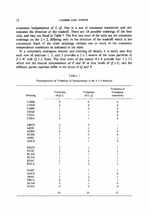
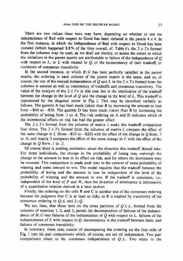
12 COOMBS AND LEHNER
consensus independence of L; Q. One is a test of consensus transitivity and one indicates the direction of the tradeoff. There are 24 possible orderings of the four cells, and they are listed in Table 7. The first two rows of the table are the consensus orderings on the 2 x 2, differing only in the direction of the tradeoff which is not consensual. Each of the other orderings violates one or more of the consensus independence conditions as indicated in the table.
In a completely analogous manner and omitting all details, it is easily seen that each row of matrices 1, 2, and 3 provides a 2 x 2 matrix of the cross partition of P X W with Q X L fixed. The four rows of the parent 4 x 4 provide four 2 X 2’s which test the mutual independence of P and W at four levels of Q x L, and the different parent matrices differ in the levels of Q and P.
TABLE 1
Decomposition of Violations of Independence in the 4 x 4 Matrices
Ordering
CADB
CDAB CABD
CBAD
CBDA CDBA
ABCD
ABDC ACBD ACDB
ADBC ADCB
BACD BADC
BCAD BCDA
BDAC BDCA
DABC DACB
DBAC DBCA DCAB DCBA
Violations Violations ofQ;L ofL; Q
Violations of
Consensus transitivity
24 24 12
0 0
0 0
0 0 1 0
1 0 1 0
0 1
1 1 0 0 0 0 1 1 1 0
1 1
2 1 1 1
1 1 2 1 2 I
1 1 1 0
2 1 2 1 1 0
2 0

ANALYSIS OF THE BILINEAR MODEL 13
As an example, consider any row of matrix 1. With Q and L held constant, decreasing the amount to win from w to w’, i.e., from $20 to $10, increases risk, and decreasing the probability of winning from p to p’, i.e., from .4 to .l, increases risk.5 Also, the diagonal comparison of the riskiness of A and D compares the incremental effect on risk of the reduction in amount to win from $20 to $10 with that of the change in probability of winning from .4 to .l in the context of a fixed level of Q and L. The four rows of matrix 1 provide four replications of this tradeoff by varying the level of Q x L, and so the independence of the tradeoff between P and W with respect to Q X L can be tested.
We see, then, that using the rows of the design, we are able to attribute the failures of independence of G; B to failure of the independence of changes in P with respect to W, of changes in W with respect to P, to inconsistency in their tradeoff, and to failure of consensus transitivity. Table 7 applies equally well to this decomposition of violations of the independence of G; B by changing the column heading Q; L to P; W and the column heading L; Q to W, P.
The results of this decomposition of the violations of independence in the parent matrices are reported next.
Results on Decomposition of Violations of Independence between Associated Variables
In a single 2 x 2 of one subject for Q x L with P x W fixed, there may be a maximum of two violations of the consensus ordering of Q with respect to L (as indicated in Table 7). With the four columns of a 4 x 4 yielding four such 2 X 2’s, and with three replications, there are a maximum of 24 violations per subject, so with 44 subjects there is a maximum of 1056. The same maxima hold for the possible number of violations of L; Q.
Violations of consensus transitivity are a maximum of 1 for each 2 X 2 for one subject, so are just one-half of the maxima for Q; L.
For the tradeoff between Q and L, revealed by the orderings on the A and D cells, there is one comparison in each 2 X 2; so, for each subject there are four 2 X 2’s which, with three replications, yield 12 orderings on A versus D. At most, 6 can go one way and 6 the other; so the maximum number of violations of the direction of dominance, whatever it might be, is 6; hence the maximum number for the total group is 264.
Because of these different maxima, we report the results (Table 8) in terms of percentages of their respective maxima. The results are reported separately for each of the three parent matrices, with the results for matrix 1 in the top row of the table and those for matrix 3 in the bottom row. The results of classifying the violations of B; G into their four sources are reported on the left side of Table 8, and the results for G; B are on the right side. The levels of Q and P are not the same in each parent 4 x 4, so their values are indicated for the convenience of the reader.
5 The ordering induced on P with W fixed is the reverse of that on Q with L fixed because p?(w) is
negative.
480/28/l-2

14 COOMBS AND LEHNER
TABLE 8
Decomposition of Violations of Independence in the Parent Matrices
Matrix
B; G G; B
Consen. Trade- Consen. Trade- Q:L L; Q trans. off P; w W, P trans. off
1 q = .l, .4 4.6 5.1 3.8 10.6 p = .l. .4 a.4 14.1 1.6 22.0 2 q = .7, .8 15.1 2.2 1.3 8.0 p=.1,.2 12.8 17.0 10.8 36.4 3 q=.1,.2 6.7 3.7 2.3 23.1 p = .7, .8 17.7 12.8 14.8 22.1
When interpreting these results, one caution must be kept in mind-the number of violations are inflated for two reasons. One is that the decomposition of a risk ordering into its constituent pair comparisons is a fine-grain unit for measuring violations. Going from a pass/fail classification of a test of independence to an integer from 0 to 6 by decomposing a rank order on four elements means the violations are not independent. A second reason is that the orderings being used against which independence is being tested is the consensus ordering (not including the ordering on A and D, cf. footnote 4). So, an individual may actually satisfy ordinary independence in the 2 x 2 and yet violate the consensus ordering and so be counted here as violating independence in the 2 x 2. We assume these inflationary effects do not bias the comparisons nor the interpretations. It is their relative magnitudes that are of interest.
In matrix 2, the change in probability of losing is from .7 to .8, and the incon- sistencies yielding violations of consensus independence is 15.1%. The same change in the probability of winning (matrix 3) has 17.7%. Comparing the change in probability of losing from .l to .2 (matrix 3) with the same change in the probability of winning (matrix 2), the corresponding percentages are 6.7 and 12.8. On the assumption that changes which are more consistently assesed are larger, these comparisons suggest that changes in the probability of losing have a more substantial effect than the corresponding changes in the probability of winning.
Comparing the change of .l in the probability of losing from .7 to .8 (matrix 2) with that from .l to .2 (matrix 3) the percentages are 15.1 and 6.7, suggesting that the change of 0.1 in the probability of losing is a greater change at low probabilities than at high probabilities. The corresponding percentages for a change of .l in the probability of winning (matrix 3 and matrix 2) are 17.7 and 12.8, suggesting that the change of .I in the pobability of winning is also a greater change at low probabilities than at high probabilities.
We see that the change in the amount to lose from -%lO to -%20 contributed less to violations of consensus independence, 2.2 and 3.7% (matrices 2 and 3, respec- tively) than the symmetric change in amount to win from $20 to $10, 12.8 and 17.0% (matrices 3 and 2, respectively), suggesting that changes in the amount to lose

ANALYSIS OF THE BILINEAR MODEL 15
have a more substantial impact on the assessment of risk than the symmetric changes in the amount to win.
We see that the change in the amounts to lose relative to the change in the probabilities of losing were more consistently assessed (2.2 versus 15.1% in matrix 2 and 3.7 versus 6.7% in matrix 3) than the symmetric change in the amounts to win versus the corresponding changes in probability of winning (12.8 versus 17.7% in matrix 3 and 17.0 versus 12.8 % in matrix 2). This suggests that a change in the amount to lose has a more substantial effect relative to the probability of losing than the symmetric change in the amount to win has relative to the corresponding probability of winning.
We also see from Table 8 that the tradeoff was the major source of violations of B; G and of G; B. In general, one would anticipate that tradeoffs would be the most difficult decisions to make because they involve resolving a conflict, whereas the other decisions are a response to monotonicity. This conflict was especially sharp for the tradeoffs between the change in the amount to win and the changes in the probability of winning.
Tradeoffs between Associated Variables
We now turn to the second value that these tests on associated variables may have. If the independence of B with respect to G is satisfied, then there are no violations of Q; L nor of L; Q, no violations of consensus transitivity, and the tradeoff between L and Q perfectly consistent; i.e., the tradeoff between a change in one variable and a change in its associated variable is independent of the level of the joint effects of the unassociated variables. So, because the tradeoff between these associated variables is consistent, we are interested in deriving the implications of the direction the tradeoff has taken.
The direction of the tradeoff is given by the risk ordering on the cells labeled A and D in Fig. 1. The gamble in cell D has been made riskier than A by the increase in the probability of losing from .l to .4. At the same time it has been made less risky than A by a decrease in the amount to lose from -%20 to -%lO. Their joint effect is revealed by the ordering on the two cells which reflects the following relation.
Consider the 2 x 2 in Fig. 1 formed from the first column of matrix 1, for which the level of (p, w) = (.l, 10). The equations for the riskiness of gambles A and D in this particular 2 x 2 are as
R(A) = 4,(-l) h(lO) + Ml) $‘I(-20)
R(D) = h(*l) f&(10) + !U4) 9,(-10).
Comparing the riskiness of A and D, we have
where >, indicates a binary risk ordering, > is on the reals, and iff means if and only if.

16 COOMBS AND LEHNER
If we change the level of P x W to any of the other three levels indicated in Fig. 1, it is obvious that we would have exactly the same relation, that D will be judged at least as risky as A if and only if the decision function, the inequality on the right, holds. This means that the model requires that the comparative riskiness of A and D cells must be the same in all four of the 2 x 2’s of Q x L obtained from the four colums of matrix 1. This test could be violated in, at most, two of the four 2 X 2’s, because there is no a priori dominance relation on these changes.
A similar analysis can be made using matrices 2 and 3 instead of matrix 1, and the decision function would be the same, differing only in the particular numerical values for the probabilities of losing taken on in those matrices (see Fig. 2a). In particular, the decision functions for the other two matrices are
matrix 2: M.8) #A-20) D ai- * iff qq.7) > d4(-10)
matrix 3: D>,A iff - 4d.2) > $d-20) M.1) ’ 44(-10) *
Note that the ratio on the right of the decision function, which we will call the threshold criterion, remains the same in all three matrices.
Exactly the same relations and interpretations, mutatis mutandis, would be found to hold for the tradeoffs in the P x W matrices. That is, in the four 2 X 2’s formed from the rows of matrix 1, the diagonal relation would point in the same direction in all four 2 X 2’s if G; B were perfectly satisfied, and the direction of the diagonal arrow indicates the relative magnitudes of the ratio of the effects of the probability of winning and the ratio of the effects of the amounts to win. Furthermore, the same test pattern would be found to hold for the 2 X 2’s formed from the rows of matrices 2 and 3, differing only in the particular numerical values of the probabilities.
The quantitative functions for the tradeoffs between associated variables, such as between Q and L or between P and W, are alike in the following respects: (i) the 2 x 2’s are formed from single arrays; (ii) the decision function only involves the two associated variables; and (iii) the direction of the tradeoff should be the same in the four 2 X 2’s. As we will see below, the decision functions for tradeoffs between unassociated variables differ from those between associated variables in all three respects, so for convenience of reference we will call these, which are between associated variables, type I tests and those between unassociated variables, type II tests.
Edwards (1962) showed that the measurement of utility and of subjective probability must be measurable on ratio scales if there are no restrictions on the sum of the subjective probabilities, and Krantz et al. (1971) pointed out, in their discussion of conditional expected utility, that the units of measurement are dependent. It is clear from the inequalities derived here that the pi must be measured on ratio scales, i.e., the additive constant of an interval scale would make these ratios

ANALYSIS OF THE BILINEAR MODEL 17
DI RECTI
-zoL-, II
1 A MATRIX I Q
El
MC 4 D LC
= h(4) > +,c-201 TOTAL LJ*;n
+,t 0 +4(-lo)
-zoL.lo
7 A MATRIX 2 Q
Ea
MC 8 0 LC
CI%A= e > 9,( 7)
+a(-201 TOTAL
+4,c-101
-20L-I0
I A MATRIX 3 a 2
Ea
MC D LC
DTAZ=Z $++ 0, (-2oj TOTAL > 3 *r(-IO)
$ OF INCR
f % -- 254 992
185 88 I
439 942
f % -- 33 140 48 314
8f 209
f %
148 607 132 644
280 62.4
SING RISK
A
H 0
f % -- 2 08
25 119
27 5.8
f % -- 202 860 105 686
307791
f % -- 96 393 73 35.6
I69 37 6
D DIRECTION OF INCREASING RISK r
.4 A MATRIX I p
D*AC&
Ea
MC
0 LC
42(20) TOTAL ) +zc IO)
.z A MATRIX 2 p
Ei
MC .t
D LC TOTAL
DhrAZ 91(.2! +2(20) +,(.I 1
2 &1101
w
MATRIX 3 p MC LC
D+A- * +2c201 TOTAL
r - hl.71 >92(10)
f %
222 98.2 144 93.5
366 96.3
f % -- 160 73 7 83 65.4
243 70.6
f %
78 33.2 37 31.1
I I5 32.5
+
A I 0
157 66.8,
FIG. 2. (a) Results of tradeoffs between probability of losing and amount to lose. (b) Results of tradeoffs between probability of winning and amount to win.

18 COOMBS AND LEHNER
arbitrary. Subsequently, it will be seen that there are dependencies among the units of measurement for all four functions in Eq. (1). These scale conditions apply to any subject matter for which this bilinear model is proposed as a theory: they are not specific to the models as a theory of risk.6
Results on Tradeofls between Associated Variables
The three panels of Figs. 2a and b represent the three matrices. On the left of each panel, the 2 x 2 and the decision function appropriate to each matrix are shown and the experimental results are shown on the right. Figure 2a refers to Q x L tradeoffs and Fig. 2b to P x W.
Note that the right-hand side of each decision function in Fig. 2a is the ratio of the effect of a loss of $20 to a loss of $10. This ratio is the same for all three matrices and is called the threshold criterion. The left-hand side of the inequality, the decision variable, is the ratio of the effects of the probabilities of losing which differ over the three matrices.
From matrix 1 it is apparent that the ratio of the effect of the probability of losing of .4 to that of .l is almost universally judged (94.2%) greater than the threshold criterion. In matrix 3, where q = .2 and .l, their relative effects exceed the threshold criterion 62.4% of the time, and in matrix 2, with q = .8 and .7, their relative effects exceed the threshold criterion only 20.9% of the time.
The corresponding results for the probability of winning (Fig. 2b) may be compared with these for the probability of losing. In the case of Fig. 2b, the right- hand side of the inequality is also a constant over the three matrices and represents the ratio of the effects on risk of the amounts to win of $20 and $10. We see that the pattern of the change from one matrix to another is very similar to that for Q x L. In the case of Q x L, the percentage of judgments indicating dominance of the change in probability was 94.2, 62.4, and 20.9. In the case of P x W, the corresponding percentages were 96.3, 70.6, and 32.5.
Comparing the results for the Q x L tradeoff with the P x W tradeoffs, the implication is that in assessing risk, the amount to lose plays a larger role relative to the probability of losing than is the case for the amount to win relative to the probability of winning.
These comparisons reinforce the conclusions drawn from the analysis of violations of independence which are reported in Table 8.
Unassociated Variables
In this section we further exploit the design to study the interrelation of unassociated variables, in this case L vs W, Q vs P, L vs P, and W vs Q. We will take
6 That behavior may reflect comparisons between ratios provides an explanation for one kind of apparently anomalous real world behavior. The risk taking behavior of an individual in one risky situation, like a high stakes poker game, may appear incompatible with the same individual’s behavior in a penny ante game, behavior that appears anomalous if one thinks in absolute terms instead of in terms
of these ratios.

ANALYSIS OF THE BILINEAR MODEL 19
QXP
(.I, .I I (.I >.4)
c.4. .I I
c.4 .tl I
FIG. 3. The L x W second order minors from matrix 1.
a particular instance, L vs W, and derive the tradeoff tests. The extension to the other cross partitions will follow readily and the results will be presented without details of derivations. The experimental results will then be presented.
Derivation of Tests of Tradeoffs between Unassociated Variables
Consider the four cells in the upper left quadrant of matrix 1 (Table 1). These cells form a second order minor with two levels of L crossed with two levels of W and with the level of Q and P, each fixed at .l. Indeed, every quadrant of matrix 1 has the same cross partition of L x W and they differ only in the level at which Q X P is fixed. The four second order minors that are formed in this way are indicated in Fig. 3. The horizontal and vertical arrows in the figure show the direction of increasing risk called consensus independence, as before, and the diagonal relation between A and D refers to the nonconsensual tradeoff between the change in L and the change in W in their effect on risk as weighted by their respective associated variables, #&) for L and o,(p) for W.
As was the case with associated variables, the value of the analysis of these second order minors is twofold. One value lies in the dissection of violations of independence of B; G and G; B in the parent 4 x 4 in terms of the failure of the mutual indepen- dence of L and W at different levels of Q X P, and the other lies in the assessment of the tradeoff between W and L as revealed by the minors when consensus indepen- dence is satisfied.
For the purpose here of assessing the bilinear model as a theory of risk, consensus independence is essential rather than the more general case of ordinary independence, and the dissection of violations of consensus independence will yield the same results as were reported for associated variables in Table 8.’ So, we devote the rest of this section to the tradeoff tests, as revealed by the direction of the arrow between cells A and D in Fig. 3.
’ In more general applications requiring discrimination within a certain class of alternative models, the dissections of the violations of ordinary independence in the second order minors would be of diagnostic value. A discussion of this would be a diversion and will not be pursued further here.

20 COOMBS AND LEHNER
In accordance with Eq. (1), we may write the riskiness of the gambles A and D in Fig. 3 for (q,p)=(.l,.l) as
R(A) = h(-l) WO) + ht.11 9d - 10)
R(D) = ht.11 hW + ht.11 94(-W.
Comparing the riskiness of A and D we have
D&A iff R(D)&R(A) iff
O,C~M(-20) -@d-WI 2 hC1)[42(10) - M20)1
and in a more convenient form for our purposes, the decision function may be written as
hC1> D&A iff - #2QO) - (6*(20) d,(*l) 2 $4(-W - O,(-10) .
The right-hand side of the inequality represents the ratio of the effect of the change in W to that of the change in L. It is important to note that the ratio on the right is a positive quantity and that it will be the same for all levels’ of Q x P; the ratio on the left-hand side of the inequality, however, will be different depending on the level of Q X P. For example, at (q, p) = (. 1, .4), we would have
4&l) D&A iff - h(lO) - M20) ht.4) a !444(-20) - 44(-10)
and similarly, the left-hand side of the inequality would become $,(.4)/#,(.1) and 93(.4)/@,(.4), for the remaining levels of Q x P from matrix 1.
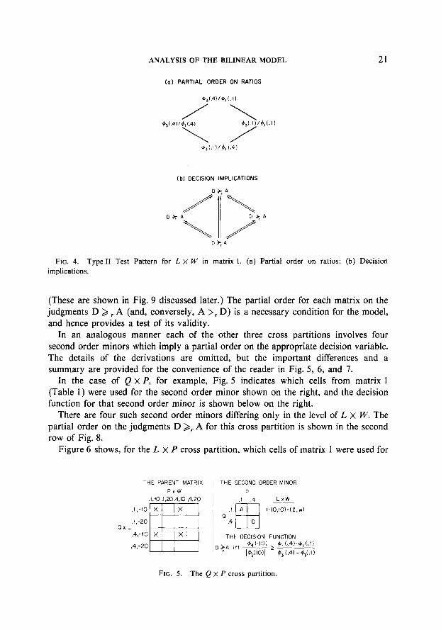
By virtue of consensus independence, i.e., the horizontal and vertical arrows in Fig. 3, we know that d,(.4) > d,(.l) and &(.4) 2 i3(.l), and hence a partial order on the decision variable is implied as shown in Fig. 4a, with the largest ratio at the top and the smallest ratio at the bottom. Figure 4b is the corresponding partial order on the responses, indicating that if D 2, A for one of the ratios, then this implies that D 2, A for all the ratios above that in the partial order.
This instance of what will be called the type II test pattern has been derived for the L x W second order minors from matrix 1. Note that only the left-hand side of the inequality changes, the decision variable; the right-hand side, the threshold criterion, is a constant for all three matrices.
If matrix 2 or 3 had served as the parent matrix for the derivation, the threshold criterion would be the same because the same levels of W and L were used, but the decision variable would take on values determined by the levels of Q and P used.
8 This constancy of the threshold criterion is a consequence of using the same experimental levels of W and L in all three matrices.
ANALYSIS OF THE BILINEAR MODEL 21
La) PARTIAL ORDER ON RATIOS
+,(.4)/+,(.0
/ \ 9,(.4V9,L4l 4&11/4,Ll)
\ / 4,(.11/9,(.41
(b) DECISION IMPLICATIONS
D h, A
FIG. 4. Type II Test Pattern for L X W in matrix 1. (a) Partial order on ratios; (b) Decision implications.
(These are shown in Fig. 9 discussed later.) The partial order for each matrix on the judgments D > r A (and, conversely, A >r D) is a necessary condition for the model, and hence provides a test of its validity.
In an analogous manner each of the other three cross partitions involves four second order minors which imply a partial order on the appropriate decision variable. The details of the derivations are omitted, but the important differences and a summary are provided for the convenience of the reader in Fig. 5, 6, and 7.
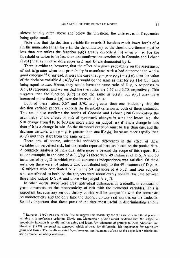
In the case of Q X P, for example, Fig. 5 indicates which cells from matrix 1 (Table 1) were used for the second order minor shown on the right, and the decision function for that second order minor is shown below on the right.
There are four such second order minors differing only in the level of L x W. The partial order on the judgments D 2, A for this cross partition is shown in the second row of Fig. 8.
Figure 6 shows, for the L x P cross partition, which cells of matrix 1 were used for
THE PARENT MATRIX THE SECOND ORDER MINOR
PXW P .I,10 .1,20.4.10 .4,20 .I .4 LXW
.I A (-10,10)=(l,w) a
.4 EH-
D OXL
THE DECISION FUNCTION
FIG. 5. The Q x P cross partition.

22 COOMBS AND LEHNER
THE PARENT MATRIX
PXW .I,10 .1,20.4.10.4.20
.I.-10 x X
.I.-20 x X QXL
.4,-10
.4.-20
THE SECOND ORDER MINOR
P ,l .4 PXW
-10 A (.I ,lO)= (q,w) L
-20 H
D
THE DECISION FUNCTION
,,,A ,ff &!?e!e > +,(.4)-+,(.1)
/ +$lO) 1 - 44(-20~~4$10)
FIG. 6. The L x P cross partition.
THE PARENT MATRIX
PXW .I.10 .I,20 A,IO cl,20
.I, -10
.I,-20 QXL
.4,-IO
.4,-20
THE SECOND ORDER MINOR
W
1020 ~ LXP
(-IO..11 =(L,p) 0
THE DECISION FUNCTION D .A ,ff +,(-lo) > +2(10’-4,(20’
14, (.I )I &(.4'-q.11
FIG. 7. The Q x W cross partition.
CROSS PARTITION lZxZ)x (2 x2’ DtA IF AND ONLY IF PARTIAL ORDER ON TESTS
dW w
LXW i
FIG. 8. Summary of type II test patterns. The prime indicates the consensual increase in risk, i.e., 0 < w’ < w, I’ < I < 0, p’ < p, q < q’, e.g., respectively, 0 < 10 < 20, -920 < 4.10 < 10. The lower the probability of losing, the greater the risk.

ANALYSIS OF THE BILINEAR MODEL 23
the second order minor shown, along with the decision function for that second order minor. The partial order on the decision variable is shown in the third row of Fig. 8.
Figure 7 and the bottom row of Fig. 8 show the same things for the cross partition Qx W.
Results on Tradeofls between Unassociated Variables
We are concerned with two aspacts of the data here, whether a partial order is satisfied in the first place, as is required by the model, and if so, the implications that may haye for the shape of the functions #i.
We assessed the degree to which a partial order on the decision variable is confirmed as follows. Note that each partial order has live linkages indicated by the double arrows (Fig. 8) but these represent relations between only four independent observations. Each of the five linkage may be confirmed, violated, or otherwise classified as indicated in Table 9.
There are alternative data bases that could be used for testing the type II partial orders. A relatively pure (and small) data base would be to use only those instances in which mutual consensus independence is satisfied by all four of an individual’s 2 x 2’s from the same parent matrix. A less pure (but larger) data base would be to use each individual 2 x 2 in which mutual consensus independence is satisfied. The data base used for Table 10 is a compromise between these two. We used those instances in which mutual consensus independence was satisfied in the 2 x 2 at each end of the linkage in the partial order; subsequently, the larger data base was used for results to be reported shortly, and the results are comparable.
The results reported in Table 10 indicate that the type II test pattern is satisfied by every pair of unassociated variables. For example, in the case of L x W, Table 10, we see that in matrix 1 there were 42.9% instances of confirmations and 1.5% instances of violations. There were another 17.9% instances of relations in the partial order that were compatible, and 37.7% of instances in which no test was possible because mutual independence of L X W was not perfectly satisfied in the individual’s 2 x 2’s at both ends of the linkage. The overall percentage of violations in Table 10 is 2.1, and the overall percentage of confirmations is 51.4, compatible 7.8, and no test was possible in the remaining 38.9%.
TABLE 9
Classification of Type II Test Outcomes for L x W
Event at (9, p) Event at (9, p’) Classification
D&A D&A A>,D A>,D
D&A A>,D A>,D D>,A
Mutual independence violated at either (9, p) or (9, p’)
Confirmation Confirmation Violation
Compatible No test possible

24 COOMBS AND LEHNER
TABLE 10
Results of Type II Tests
Confirmations Violations Compatible No test
possible
f % f % f % f
LXW
Matrix 1 Matrix 2 Matrix 3
LXP Matrix 1 Matrix 2 Matrix 3
QxW Matrix 1 Matrix 2 Matrix 3
QxP Matrix 1 Matrix 2 Matrix 3
283 42.9 IO 1.5 118 17.9 249 37.7 316 57.0 2 0.3 9 1.4 213 41.4 397 60.2 18 2.7 36 5.5 209 37.1
366 55.5 4 0.6 112 17.0 178 27.0 379 57.4 20 3.0 14 2.1 247 31.4 325 49.2 13 2.0 66 10.0 256 38.8
360 54.5 6 0.9 43 6.5 251 25.6 235 35.6 18 2.7 51 7.7 356 48.3 368 55.8 27 4.1 26 3.9 239 44.2
392 59.4 17 2.6 82 12.4 169 25.6 212 41.2 18 2.7 51 7.7 319 48.3 321 48.6 10 1.5 47 7.1 292 44.2
%
In judging the statistical significance of these results, we note that the live linkages indicated by the five arrows in each partial order of Fig. 8 are not independent. Furthermore, we see in Table 9 that there are two ways in which a linkage may be confirmed and only one way in which it may be violated. The overall ratio of conlir- mations to violations in Table 10 is about 24 to 1 in contrast to 2 to 1 on a random basis, indicating that the independence conditions between unassociated variables are satisfied as required by the model.
The results for the MC group and the LC group are not reported separately in order not to burden the reader unnecessarily. The results for the LC group alone were about 17 to 1 confirmations to violations. The main difference between the two subgroups is that the LC group contributed 75% of the instances in which no test was possible.
Given that a type II partial order is satisfied as required by the model, then the direction of the risk ordering between A and D has significance for the relative shapes of the functions #i. The particular implications depend on the contrasts involved in a particular cross partition and its partial order. Consequently, we discuss the results on each partial order separately. The nature of the data base and the

ANALYSIS OF THE BILINEAR MODEL 25
statistical model used for this purpose is the same for all four partial orders, so it is presented in detail only in the discussion of the first cross partition.
LXW
The decision variable, the threshold criterion, and the partial order for this cross partition are presented in the first row of Fig. 8. The decision variable for L x W is the ratio of the effects of q and p, $3(q)/#1(p), an is shown on the left-hand side of d the inequality. The threshold criterion is the ratio of the effects of the changes in winning and losing, and is shown as the right-hand side of the inequality. As the levels of p and q are changed, the decision variable is changed without changing the threshold criterion. Hence, the change in the decision variable alone determines whether a change occurs in the judgment as to which is riskier, A or D, and, of course, this may not be the same for different individuals.
Because the threshold criterion for this cross partition, L x W, is the same for all three matrices, we may interlock the three partial orders from the three matrices into a common partial order, as shown in Fig. 9, where the number in parentheses indicates the parent matrix. We see that the partial order from matrix 2 forms the top of Fig. 9, and the partial order from matrix 3 forms the bottom, with matrix 1 interlocking with each of them at two points. The largest value of the decision variable is at the top of the partial order and the smallest at the bottom. The decision function is included at the bottom of the figure for the convenience of the reader.
The interlocked partial order permits testing, whether or not the data from all three matrices are compatible with the model, not only within each matrix, but between
+&I)/d,l.a) 13) 46,59,27, 1.28
(I),(Zl,l3). DECISION FUNCTION
FIG. 9. Interlocking the partial orders of L x W from matrices 1, 2, and 3.

26 COOMBS AND LEHNER
them. For this purpose, the data base was broadened from that which was used for Table 10.
The data base for Table 10 was conditional on mutual consensus independence being satisfied in a pair of 2 x 2’s, those at the two ends of an implication (arrow). Furthermore, the pair of 2 x 2’s were from the same parent matrix. In testing the interlocked partial order, some of the 2 x 2’s forming a pair would be from different parent matrices, and to have required that mutual consensus independence be satisfied by a pair of 2 x 2’s from different parent matrices would have severely reduced the data base. This provided an opportunity to explore a different statistical model using a larger data base.
Consequently, the data base for Fig. 9 is expanded by using all the 2 x 2’s, which satisfied mutual consensus independence for that 2 x 2 in the partial order. This broader base also provides a check on the results in Table 10, which used a smaller base.9
The data base used for the interlocked partial order requires a different statistical model and a different form for reporting the results.
The statistical model on which the interpretations are based is as follows: at each point in the partial order there corresponds an urn with two kinds of chips in it. One kind has printed on them the event A >,. D and the other kind says D 2,. A. When a chip is drawn from the urn, however, it may not be readable. It is assumed that every chip has an equal probability of being drawn and has an equal probability of being readable. The ratio of the two kinds of readable chips provides an estimate of the ratio of their relative proportion in each urn and thereby tests the partial order and implies an ordering on the otherwise incomparable pairs.
The results are reported in Fig. 9 as follows: At each point in the interlocked partial order, the number of the matrix is in parentheses and is followed by three integers and sometimes a fourth number which is a decimal. The first integer is the raw frequency of the event A >,, D. The second integer is the frequency of the event D >, A, and the third integer is the frequency of the failure of mutual consensus independence in that 2 x 2. These three numbers add up to 132, which is the number of replications of the second order minor (3 replications times 44 subjects) at each point in every partial order. The fourth number, a decimal, is a ratio of the frequency of the event D >, A divided by the frequency of the event A >r D. No ratios are calculated, however, if the frequency in the denominator is less than 5. There are three instances in Fig. 9 with frequencies of 1, 2, and 4, all in matrix 2 at the top of the interlocked partial order.
These ratios should decrease from top to bottom of the partial order because the threshold criterion is a constant and the decision variable is decreasing. An X on a linkage in the partial order indicates a violation. There are three in Fig. 9, all involving matrix 3, including one between it and matrix 1. Note that the ratios for these linkages are close to one, indicating that the value of the decision variable was
9 The only differences observed are attributable to the higher noise level that accompanied the broader base.
ANALYSIS OF THE BILINEAR MODEL 21
almost equally often above and below the threshold, the differences in frequencies being quite small.
Note also that the decision variable for matrix 3 involves much lower levels of q (in the numerator) than for p (in the denominator), so the threshold criterion must be less than one unless the function &(q) greatly exceeds 4,(p) when q = p. For the threshold criterion to be less than one confirms the conclusion in Coombs and Lehner (1981) that symmetric differences in L and W are dominated by L.
There is evidence, however, that the effect of a given probability on the assessment of risk is’greater when that probability is associated with a bad outcome than with a good outcome. lo If instead, it were the case that q = p 5 &(q) = g,(p), then the value of the decision variable #,(.4)/9,(.4) would be the same as that for &(.l)/$,(.l), each being equal to one. Hence, they would have the same ratio of D >, A responses to A >r D responses, and we see that the two ratios are 5.67 and 3.70, respectively. This suggests that the function &(q) is not the same as #l(p), but 9,(q) may have increased more than o,(p) over the interval .l to .4.
Both of these ratios, 5.67 and 3.70, are greater than one, indicating that the decision variable generally exceeds the threshold criterion in both of these instances. This result also confirms the results of Coombs and Lehner (198 1) indicating the asymmetry of the effects on risk of symmetric changes in wins and losses; e.g., the $10 change from $10 to $20 has more effect on judged risk if it is a change in loss than if it is a change in win. So the threshold criterion must be less than one, and the decision variable, with p = q, is greater than one if ti3(q) increases more rapidly than g,(p) and they start from the same origin.
There are, of course, substantial individual differences in the effect of these variables on perceived risk, but the results reported here are based on the pooled data. A complete analysis of individual differences is beyond the scope of this report. But as one example, in the case of #3(. 1)/#,(.7) there were 49 instances of D >, A and 50 instances of A >r D in which mutual consensus independence was satisfied. Of these instances there were 14 subjects who contributed only to the 49 instances of D >, A, 16 subjects who contributed only to the 50 instances of A >r D, and four subjects who contributed to both, so the subjects were about evenly split in this case between those who judged D >, A and those who judged A >r D.
In other words, there were great individual differences in tradeoffs, in contrast to great consensus on the monotonicity of risk with the elemental variables. This is important because any serious theory of risk will be compatible with the consensus on monotonicity and the only time the theories do any real work is on the tradeoffs. So it is important that those parts of the data most useful in discriminating among
lo Edwards (1962) was one of the first to suggest this possibility for the case in which the dependent
variable is a preference ordering. Slavic and Lichtenstein (1968) report evidence that the subjective probability function is conditional on gains and losses for judgments of preference. Also Anderson and Shanteau (1970) presented an approach which allowed for differential felt importance for equivalent
gains and losses. The results reported here, however, use judgments of risk as the dependent variable and not preference or utility orderings.

28 COOMBS AND LEHNER
theories be isolated and not drowned in the effects of monotonicity; which is exactly what this experimental design and the conjoint measurement tests developed here are designed to do.
QxP The second row of Fig. 8 displays the type II test pattern for the Q X P partition.
The decision variable is shown on the left-hand side of the inequality, and the threshold criterion is shown on the right-hand side of the inequality. In this cross partition, in contrast to the preceding, the decision variable is the same for all three matrices, and it is the threshold that is different for each. The result of this is that interlocking the three partial orders from the three matrices merges them as shown in Fig. 10. Below the figure, the decision function is given for each matrix for the convenience of the reader.
The numbers in the figure have the same referents as in Fig. 9, the number in parentheses being the matrix number, and then in turn, the frequency of A >,. D, D 2, A, the number of failures of mutual consensus independence, and the ratio of the first two frequencies. The larger this ratio is the higher the proportion of D >, A and so the lower must be the threshold.
For each matrix the partial order on the decision variable must be satisfied, i.e., the ratio must decrease from top to bottom of the partial order. For example, for matrix 2 we see that the ratio at the top of the partial order is 2.40, at the bottom it is 1.10, and the other two values are in between. We see that the same pattern holds in all three matrices, as is required. This confirms the results for this cross partition reported in Table 10 in which a purer but smaller data base was used.
In addition to this test within matrices, there is a between matrices test. At each
DECISION FUNCTIONS
FIG. 10. Interlocking the partial orders of Q x P from matrices 1, 2, and 3.
ANALYSIS OF THE BILINEAR MODEL 29
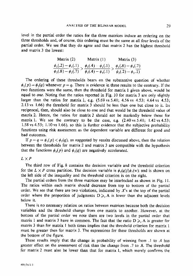
level in the partial order the ratios for the three matrices induce an ordering on the three thresholds and, of course, this ordering must be the same at all four levels of the partial order. We see that they do agree and that matrix 2 has the highest threshold and matrix 3 the lowest:
Matrix (2) Matrix (1) Matrix (3)
h(*2)-h(*l) > $,(-4)-#,(.1) > #,(*9-$,(*7) 43(J) - M.7) 43(.4)-43(.1) ~~4.2) - 43.1)
The ordering of these thresholds bears on the substantive question of whether b,(p) = 43(q) h w enever p = q. There is evidence in these results to the contrary. If the two functions were the same, then the threshold for matrix 1 given above, would be equal to one. Noting that the ratios reported in Fig. 10 for matrix 3 are only slightly larger than the ratios for matrix 1, e.g. (5.69 vs 5.41; 4.56 vs 4.53; 4.64 vs 4.53; 2.13 vs 1.66) the threshold for matrix 3 should be less than one but close to it. Its reciprocal, then, should also be close to one and that would be the threshold value of matrix 2. Hence, the ratios for matrix 2 should not be markedly below those for matrix 1. We see the contrary to be the case, e.g. (2.40 vs 5.41; 1.42 vs 4.53; 1.58 vs 4.53; 1.10 vs 1.66), so this is further evidence that the subjective probability functions using risk assessment as the dependent variable are different for good and bad outcomes.
Ifp= 4* #l(P) < M4h as suggested by results discussed above, then the relation between the thresholds for matrix 2 and matrix 3 are compatible with the hypothesis that the functions Q,(p) and &(q) are negatively accelerated.
LXP The third row of Fig. 8 contains the decision variable and the threshold criterion
for the L x P cross partition. The decision variable is #3(q)/1#2(w)j and is shown on the left side of the inequality and the threshold criterion is on the right.
The partial orders from the three matrices may be interlocked as shown in Fig. 11. The ratios within each matrix should decrease from top to bottom of the partial order. We see that there are two violations, indicated by X’s at the top of the partial order where the proportion of judgments D >, A is lower than the adjacent levels below it.
There is no necessary relation on ratios between matrices because both the decision variables and the threshold change from one matrix to another. However, at the bottom of the partial order we note there are two levels in the partial order that matrix 1 and matrix 3 have in common. The fact that the ratio D >, A is greater for matrix 3 than for matrix 1 both times implies that the threshold criterion for matrix 1 must be greater then for matrix 3. The expressions for these thresholds are shown at the bottom of the figure.
These results imply that the change in probability of winning from .l to .4 has greater effect on the assessment of risk than the change from .7 to .8. The threshold for matrix 2 must also be lower than that for matrix 1, which merely confirms the
480/28/l-3

30 COOMBS AND LEHNER
4,(.81114,(1011 (21 20,78.34.3.90
4~Lll/14,(20~~ ~094.l1,27,0.12) (3)40,61,31.1.53
DECISION FUNCTIONS
I,,D+!e4Jo- > 4,(.41-4,i.ll
1421wll - 4~4(-201-44(-10)
(2, o*;ese4& ? 4,(.21-4,f.l 1
4.,(-20)-4a4(-10)
4,(q) 4,(.8l-4,(.71
L3’ “* ==m ’ 4,l-201.4,(-to1
FIG. Il. Interlocking the partial orders of L x P from matrices 1, 2, and 3.
monotonicity of 4,. The threshold for matrix 2 cannot be compared with that for matrix 3 because the values of the decision variables are higher than those for matrix 3. So the higher frequencies of D >, A and the lower frequencies of A >r D could be accounted for by either effect.
QxW The last row of Fig. 8 shows the Q x W partition. The partial orders on the
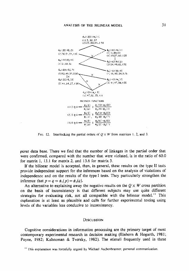
decision variable, 44(Z)/#1 (p), may be interlocked from the three matrices, as shown in Fig. 12. The threshold criterion for this cross partition is different for each matrix and they are provided at the bottom of the figure for the convenience of the reader.
There are three instances in Fig. 12 of frequencies below 5 in the denominator; they are 0, 2, and 3, so these were not used in calculating ratios. There are four X’s indicated in the figure for matrix 3, and one for matrix 2. The results on this partial order are very unsatisfactory from the point of view of the bilinear model. In this cross partition the threshold criterion is a change in the effect of the amount to win divided by a change in the effect of the probability of losing. We have seen that the effect of the amount to win was a major source of inconsistency in judging risk, and the change in the probability of losing was only .l in matrices 2 and 3. So it is not unreasonable that this threshold might be exceptionally variable. In matrix 1, for example, the change in probability of losing is from .l to .4 and the data are much more consistent (Table 4).
These interpretations are supported by the results reported in Table 10 based on a
ANALYSIS OF THE BILINEAR MODEL 31
+4 I-20) /C,l II (I 13.92,37 l2)25,64.43.2 56
DECISION FUNCTIONS
FIG. 12. Interlocking the partial orders of Q X W from matrices 1, 2, and 3.
purer data base. There we find that the number of linkages in the partial order that were confirmed, compared with the number that were violated, is in the ratio of 60.0 for matrix 1, 13.1 for matrix 2, and 13.6 for matrix 3.
If the bilinear model is accepted, then, in general, these results on the type II tests provide independent support for the inferences based on the analysis of violations of independence and on the results of the type I tests. They particularly strengthen the inference that p = q * #l(p) = 43(q).
An alternative to explaining away the negative results on the Q X W cross partition on the basis of inconsistency is that different subjects may use quite different strategies for evaluating risk, not all compatible with the bilinear model.” This explanation is at least as plausible and calls for further experimental testing using levels of the variables less conducive to inconsistency.
DISCUSSION
Cognitive considerations in information processing are the primary target of most contemporary experimental research in decision making (Einhorn & Hogarth, 1981; Payne, 1982; Kahneman & Tversky, 1982). The stimuli frequently used in these
” This explanation was forcefully argued by Michael Aschenbrenner, personal communication.

32 COOMBS AND LEHNER
studies, and to which we will confine our attention in this discussion, are gambles or portfolios of gambles (consisting usually of two gambles).
The tasks subjects are asked to perform are typically an assessment of risk or preference using as a response mode some instance of the method of single stimuli such as a rating scale or absolute judgment, or using some instance of the method of choice, like pair comparisons (see Coombs, 1964, Chap. 2 for their variety and some formal relations among them).
A characteristic of this research is that some standard of rational behavior exists, such as Bayes theorem or expected utility principles, or other objective standards derived from first principles which are accepted a priori. The failure of subjects’ behavior to meet such standards is one of the forces driving this research for the past 10-15 years.
The experiments of Slavic (1967), Slavic and Lichtenstein (1968) and Anderson and Shanteau (1970) made extensive use of what they called duplex gambles which were portfolios of gambles in which the component gambles were of a particular kind (see below). The experiments of Lindman (1971) and Payne and Braunstein (1971), using portfolios of gambles that were constituted differently but were formally equivalent in final outcomes and probabilities, demonstrated reversals of preference, an inconsistency incompatible with conventional standards of rationality.
Most important of all have been the contributions of Kahneman and Tversky which have given coherence and direction to this research with their demonstration of regularities in the departures from the a priori standards of rationality. They account for these regularities in terms of heuristics and biases induced by the framing of the task. The existence of empirical regularities which may be experimentally controlled and manipulated implies the existence of underlying laws and principles, and in this sense the behavior is rational and rigorous theory can exist. The paper by Kahneman and Tversky (1981) and the book by Kahneman, Slavic, and Tversky (1982) provide an introduction and review of this literature.
The dissection and testing of the cognitive processes in these judgment and choice tasks is aided by further enriching the stimulus domain, which can be done in a systematic manner. A portfolio may, on the one hand, be presented in its most elemental form as a set of final outcomes and probabilities. On the other hand, the gambles comprising a portfolio may themselves be presented and constitute the experimentally independent variables that are manipulated. If the independent variables are themselves gambles, then the tradeoffs being studied by the methodology developed here would be tradeoffs between the contributions of gambles to a portfolio instead of tradeoffs between the elemental variables used in this experiment.
This form of presentation, using gambles as the independent variables, implicitly introduces intermediate stages in the processing of information in a manner which is under the control of the experimenter. There are, in some cases, as will be seen, an infinite variety of alternative ways of phasing the process and this can be a powerful tool for both theoretical psychology and applied decision making. The variety of distinct representations, all equivalent in final outcomes and probabilities, permits

ANALYSIS OF THE BILINEAR MODEL 33
varying the salience of the elemental components and the distribution of attention and thereby inciting different heuristics and biases in the search for regularities.
It is important to keep in mind, in the background, that tradeoffs remain, at the heart of all decision making, and that the methods developed in this paper are directed at the fine-grain study of tradeoffs. The experiments reported here have been based on tradeoffs between the elemental variables, outcomes, and probabilities, but the methodology applies equally well whether the independent variables are the constituent gambles of a portfolio, or the task is assessment of risk or preference. and/or the response mode uses a method of single stimuli or a method of choice.
We began the systematization of this stimulus domain using gambles as the independent variables in a portfolio, with the early work on duplex gambles. A duplex gamble is a pair of gambles in which one consists of an amount to win at a specified probability, otherwise nothing, and the other consists of an amount to lose at a specified probability, otherwise nothing. It is understood by the subject that both gambles are to be played independently, and together constitute a single stimulus.
The data in the early experiments were analyzed by linear regression and analysis of variance using the values of probability and amounts of money that had been displayed to the subject. Conclusions were drawn about the relative importance of outcomes and probabilities on strength of preference and on riskiness, for example, that “‘the probability of loss’ was the most important single determiner of perceived risk; and the ‘amount to lose’ was far less important” (Slavic, 1967).
In terms of final outcomes and probabilities each duplex gamble, of course, corresponds exactly to a single gamble with three or four possible outcomes. In the experiments by Slavic and by Slavic and Lichtenstein, 9 of the 27 duplex gambles used corresponded to three-outcome gambles, and the remaining 18 corresponded to four-outcome gambles. As an illustration, an example of a duplex gamble (taken from Slavic, 1967, Fig. 1) is shown at the top of Fig. 13. In terms of final outcomes and probabilities, this duplex gamble is equivalent to the four-outcome games shown in the middle of Fig. 13. We will refer to this procedure of playing both gambles experimentally independently as compound composition symbolized in the figure by 0.
The four-outcome gamble resulting from the compound composition of two two- outcome gambles can be decomposed into an infinite number of pairs of two-outcome gambles. One such possible decomposition is shown in the bottom of Fig. 13.
The heart of the issue is that, if the subject’s assessments vary in any systematic manner over equivalent decompositions of the same four-outcome gamble, then any model using only final outcomes and probabilities as variables can, at best, only account for behavior in response to stimuli presented in the form of final outcomes and probabilities. All decompositions disguise the final outcomes and probabilities, and this can only impede their usefulness for the purpose of assessing the contributions of outcomes and probabilities to the evaluation of a gamble, whether it be its attractiveness or its riskiness.
For example, one of the duplex gambles that has been used in several studies is the following: ($1, .8: 0, .2) and (0, .6; -$l, .4), i.e., to win $1 with probability .80.
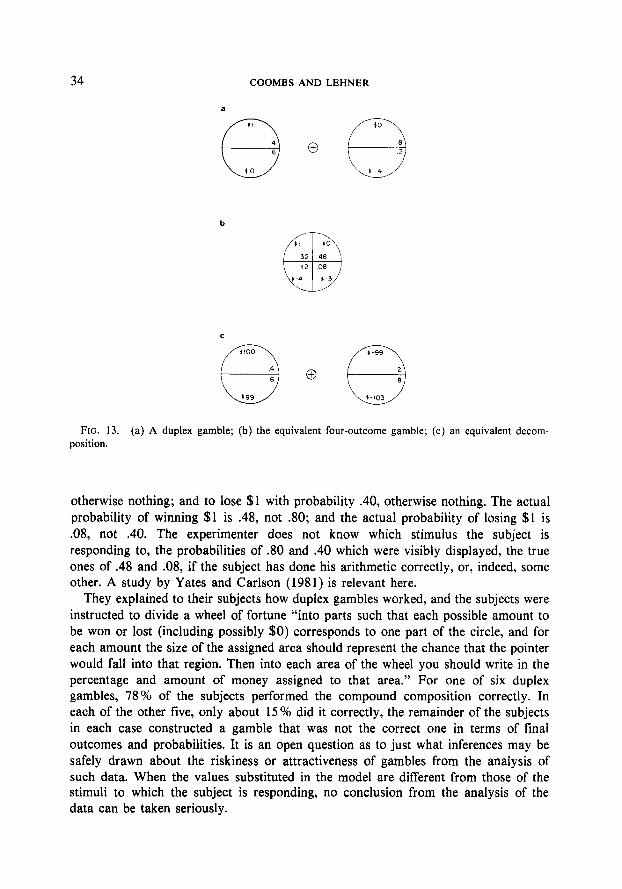
34 COOMBS AND LEHNER
b
FIG. 13. (a) A duplex gamble; (b) the equivalent four-outcome gamble; (c) an equivalent decom- position.
otherwise nothing; and to lose $1 with probability .40, otherwise nothing. The actual probability of winning $1 is .48, not .80; and the actual probability of losing $1 is .08, not .40. The experimenter does not know which stimulus the subject is responding to, the probabilities of .80 and .40 which were visibly displayed, the true ones of .48 and .08, if the subject has done his arithmetic correctly, or, indeed, some other. A study by Yates and Carlson (1981) is relevant here.
They explained to their subjects how duplex gambles worked, and the subjects were instructed to divide a wheel of fortune “into parts such that each possible amount to be won or lost (including possibly $0) corresponds to one part of the circle, and for each amount the size of the assigned area should represent the chance that the pointer would fall into that region. Then into each area of the wheel you should write in the percentage and amount of money assigned to that area.” For one of six duplex gambles, 78% of the subjects performed the compound composition correctly. In each of the other five, only about 15% did it correctly, the remainder of the subjects in each case constructed a gamble that was not the correct one in terms of final outcomes and probabilities. It is an open question as to just what inferences may be safely drawn about the riskiness or attractiveness of gambles from the analysis of such data. When the values substituted in the model are different from those of the stimuli to which the subject is responding, no conclusion from the analysis of the data can be taken seriously.

ANALYSIS OF THE BILINEAR MODEL 35
In the derivations of the decision functions for the various tradeoffs in the general bilinear model using outcomes and probabilities as the variables, we have seen that the decision reflects an inequality between two ratios. In the case of the tradeoff between two associated variables, like probability of losing and amount to lose, the subject is responding to a ratio of the effects of two probability levels for losing to a ratio of the effects of two amounts to lose (Fig. 8 summarizes these relations).
One of the consequences of this is that conclusions that one variable is more important than another may have little generality beyond the levels used in the particular experiment.” For example, in results reported earlier (Fig. 2), we saw that the change in the amount to lose from 410 to -420 dominated the change in the probability of losing from .7 to .8, but was dominated by the change from .l to .2. It is meaningless, then, to say without precise qualification that the amount to lose is more or less important than the probability of losing.
A similar relation held for the effect of the change in the amount to win from $20 to $10 which dominated the change in the probability of winning from .8 to .7, but was dominated by the change from .2 to .l. The degree of domination differed consis- tently, however. It was as if in assessing risk, the amount to lose plays a larger role relative to the probability of losing than the amount to win does relative to the probability of winning. There is no justification evident for stronger or more general conclusions.
To summarize the discussion up to here, we have seen that duplex gambles, or any other decomposed form, misrepresent and, in fact, may severely distort the actual outcomes and probabilities. Hence, their use in experiments to study models which have final outcomes and probabilities as variables or to answer questions about the relative importance of outcomes and probabilities in the assessment of gambles is, to say the least, not recommended. Furthermore, if the assessment of gambles is considered to be a bilinear function of the outcomes and probabilities, or any of its special cases, then the behavior is a response to a relation on ratios and questions about the relative importance of outcomes and probabilities are not generally meaningful.
Most studies have been directed at modeling the assessment of gambles in terms of final outcomes and probabilities and not with the study of behavior over equivalent decompositions (important exceptions are the papers by Aschenbrenner (1978) and many of the studies by Kahneman & Tversky (e.g., 1979)). However, if individuals when presented with a decomposed portfolio responded to it veridically in terms of final outcomes and probabilities, then the use of one form of display or another would make no difference. If, however, behavior is not consistently compatible under all forms of display, then models of assessment, whether risk or preference, must introduce other psychological concepts, such as attention and set, salience, sequential processing effects, arithmetic biases, simplifying heuristics, to account for the failure of veridical behavior. In such cases, duplex gambles, and more generally, the entire
‘* The same reservation applies to conclusions about the risk-taking propensities of individuals; see footnote 6.

36 COOMBS AND LEHNER
range of alternative equivalent decompositions, make possible the systematic and controlled experimental study of biases and heuristics and the decomposition of cognitive processes.
We discuss two types of stimulus decomposition, compound and contingent, in that order.
The necessary and sufficient conditions for the existence of a compound decom- position of a four-outcome gamble with outcomes 0, > 0, > 0, > O,, with associated probabilities p, , p2, p3, p4, respectively, are
(i) 0, + 0, = 0, + 0,
6) PI P4 = P2P3.
If the compound decomposition is designated (x, r; y, 1 - r) and (v, S; w, 1 - s), where x and y are outcomes with probabilities r and 1 - r, respectively; and z, and w are outcomes with probabilities s and 1 - S, respectively, then a decomposition exists in which
o,=x+v p, = rs
o,=x+w p2 = r(1 - s)
o,=y+v p3=(1-r)s
o,=y+w p4=(1 -r)(l-s)
where exactly one of x, y, v, w is arbitrary. Hence the number of distinct decom- positions is infinite. There is no freedom in the choice of the probabilities r and s.
If exactly one of the outcomes equals zero, then another equals the sum of the remaining two. In particular, if y = -v = 0, then 0, = 0, and the corresponding decomposition is a duplex gamble and it is unique. So the existence of a duplex gamble puts a substantial constraint on the range of four-outcome gambles which may be studied by compound decomposition.
Contingent composition refers to the display of two gambles in which one is to be played with some probability, say t, and the other is to be played with probability (1 - t). Any four-outcome gamble with outcomes Or, 0,) 0,) 0, and with associated probabilities p, , p2, p3, p4, respectively, can be contingently decomposed in exactly three ways:
6) [O,,p*; 029-j-$--]T t= PI + P2; I 2 1 2
I O,,A P3 + P4
; o,,A I P3 + P4 ’
1 -t=pj+p4*

ANALYSIS OF THE BILINEAR MODEL 37
(ii) [0,,*;03~-/$-J, t=pI+p3; 1 3 1 3
I
O,,A P2 + P4
;o,,P” , P2 + P4 I
1-t=pp,+p,.
(iii) [Olyp+; 04,-5---j, t= P, + p4; I 4 1 4
I 02, p2
p3 -; o,,- P2 + PJ Pz + P, I ’
1-t=pp,+p,.
As an example, the four-outcome gamble shown in Fig. 13 can be contingently decomposed exactly three ways as shown in Fig. 14. If behavior is a function of final outcomes and their probabilities only, then the behavior should be invariant over these alternative displays, and also remain invariant over the compound decom- positions of that four-outcome gamble, two of which are shown in Fig. 13. Systematic departures from invariance should be a rich source for insight into hypotheses about the decision processes.
Evidence of the existence of systematic departures from invariance was reported in a study by Coombs and Bowen (1971) in which compound and contingent compositions were compared with respect to additivity of the riskiness of the resulting portfolio. The stimuli were displayed decomposed and also in terms of final outcomes. There were substantial differences; for example, additivity of risk in a
FIG. 14. The three contingent decompositions of the gambles in Fig. 13.

38 COOMBS AND LEHNER
portfolio was clearly violated for compound composition with the stimuli displayed in terms of final outcomes and their probabilities, whereas under contingent composition this was not the case. With the portfolios displayed decomposed, there was little difference between compound and contingent composition, as if the subjects disregarded information about the composition function.
Another basis for anticipating systematic differences in behavior over decom- positions equivalent in final outcomes and probabilities is found in the following thought experiment. Consider the gambles shown in Fig. 15.
At the top of the figure is a duplex gamble, labeled A, for winning and losing $10. Both are to be played, i.e., compound composition. Below A in the figure is the four- outcome gamble, labeled B, which is equivalent to A in terms of outcomes and probabilities (it is actually a three-outcome gamble, but is displayed as a four- outcome gamble for the convenience of the reader). At the bottom of the figure are two different contingent decompositions, C and D, of the four-outcome gamble B. All four gambles, A, B, C, and D, are identical in final outcomes and probabilities.
Note that gambles A and C have identical components, but in A both are to be played and in C only one. It is doubtful that subjects who are not mathematically inclined will respond identically to them.
Equivalent compound and contingent decompositions like A and C will occur whenever 0, is greater than zero, 0, and 0, both equal zero, 0, equals minus 0,) and their respective probabilities are p*, pq, pq, q2.
Finally, we mention a still different form of presentation which was used by
FIG. 15. Equivalent compound and contingent decompositions.

ANALYSIS OFTHE BILINEARMODEL 39
Aschenbrenner (1978). He reports an experimental study comparing preferences for simple two-outcome gambles under two modes of presentation. One mode was in terms of final outcomes and probabilities, and the other mode was in terms of a wager in which the player has to pay a stake y to play the gamble to win x + y with probability p. The gambles presented in the latter mode were identical to those presented under the former mode in terms of final outcomes and their probabilities.
In spite of this identity, preferences were different in the two sets, satisfying single peaked preference functions in the stake presentation mode and violating single peakedness under final outcomes presentation. He had predicted these differences in that the set presented in terms of final outcomes and their probabilities did not constitute an efftcient set and under stake presentation they did.
The stake presentation mode offers another approach to constructing a set of gambles equivalent to another set in terms of final outcomes and probabilities, but predictably not equivalent in terms of preference. As Aschenbrenner puts it, “. . . formally irrelevant aspects of presentation can make a big difference in preference,. . . challenging the core of every ‘rational’ theory of decision making” (1978, p. 5 16).
SUMMARY
The bilinear model, perhaps the most widely applied model in behavioral science, has not previously been open to study in detail by conjoint measurement methods although Anderson and Shanteau (1970) have extended functional measurement to the analysis of this model for a different experimental design, one in which the independent variables are duplex gambles.
The experimental design and the method of analysis developed here are ones in which the independent variables are not themselves gambles, but are terms in a bilinear equation. The tests for this design are measurement-free in the sense that only ordinal properties of the dependent variable are used and only ordinal conditions on the independent variables are tested.
Numerical scales more powerful than ordinal would be more sensitive, and lead to stronger conclusions, of course, but the tests derived here reveal that ratio scales would be required for all the independent variables and, furthermore, their units of measurement would be interdependent. Such requirements encourage the development of measurement-free tests.
Using a (2 X 2) x (2 X 2) experimental design, new tests are developed for the mutual independence and tradeoffs between variables associated within the same term of the model, like an outcome and its associated probability, e.g., an amount to win and the probability of winning; and between variables from different terms, called unassociated variables, e.g., the amount to win and the probability of losing, or the amount to win and the amount to lose.
These tests may be used to detect the locus and cause of each violation of the model and, in the absence of violations, to provide information about the shape of the functions which measure the contribution of each independent variable. Serious

40 COOMBS AND LEHNER
statistical problems emerge as with other conjoint measurement procedures, but ad hoc procedures and controls are devised which offer some justification for the inferences drawn.
Findings include the following:
(1) Risk orderings are decomposable into contributions from good and bad components which are additive in their joint effect. The good component (the joint effects of the probability of winning and the amount to win) plays a lesser role than the bad component (the joint effect of the probability of losing and the amount to lose) in the assessment of risk when the probabilities of winning and losing are matched (.l, .2, .4, .7, .8) and the amounts to win and lose are matched in absolute value ($10 and $20).
(2) The pattern revealed by the decomposition of violations of independence between associated variables (like P and W and like Q and L) was supported by the pattern of tradeoffs between changes in associated variables (like an increase in the probability of losing versus an increase in the amount to lose). The results suggested the following conclusions:
(i) A change in the probability of losing had a more substantial effect than the corresponding change in the probability of winning.
(ii) A change of 0.1 in probability had more effect at low probabilities (. 1 to .2) than at high probabilities (.7 to .S).
(iii) A change in amount to lose had a more substantial effect than the corresponding change in amount to win relative to the same values of the associated probabilities.
(3) Analysis of the tradeoffs between unassociated variables W& L, P & Q, P & L satisfied the bilinear model but those between Q & W raise a serious question about the validity of the model for the assessment of risk. Two possible explanations for the failure of the model were based on the inconsistency induced by small differences in the experimental variables and by the use of alternative strategies for assessment of risk which are not compatible with the bilinear model. The latter explanation is the more plausible insofar as the data of this experiment are concerned.
(4) An experimental procedure involving the presentation of a portfolio as a composite of gambles instead of a set of final outcomes and probabilities is discussed. Two forms of composition, compound and contingent, are formulated and illustrated. They are shown to distort the true final outcomes and probabilities and hence incite biases and heuristics and expose the cognitive processes involved in decision making.
(5) Finally, the decision functions under the bilinear model using final outcomes and probabilities reveal that the behavior must be a response to relations between ratios of the effects of the elemental variables and ratios of the effects of differences between levels of the elemental variables. This is shown to have substantial effect on the inferences that may be drawn.

ANALYSIS OF THE BILINEAR MODEL 41
REFERENCES
ANDERSON, N. H. Information integration theory: A brief summary. In D. H. Krantz, R. C. Atkinson, R. D. Lute, & P. Suppes (Eds.), Contemporary developments in mathematical psychology (Vol. 2). San Francisco: Freeman, 1974.
ANDERSON, N. H., & SHANTEAU, J. C. Information integration in risky decision making. Journal of
Experimental Psychology, 1970, 84, 441-45 1. ASCHENBRENNER, K. M. Single-peaked preferences and their dependability on the gamble’s presentation
mode. Journal of Experimental Psychology: Human Perception and Performance, 1978, 4, 513-520. ATKINSON. J. W. Motivational determinants of risk-taking behavior. Psychological Review, 1957, 64(6),
359-372. BERLINER, H. Chess as problem solving: The development of a tactics analyzer. Unpublished doctoral
thesis, Carnegie-Mellon University, 1974. COOMSS. C. H. A theory of data. New York: Wiley, 1964. Reissued by Mathesis Press, Ann Arbor,
Michigan, 1976. COOMBS. C. H.. & BOWEN. J. Additivity of risk in portfolios. Percepfion and Psvchophysics, 1971, IO,
4346. COOMBS. C. H., & LEHNER, P. H. Evaluation of two alternative models for a theory of risk: I. Are
moments of distributions useful in assessing risk? Journal of Experimental Psychology: Human
Perception and Performance, 1981, 7, 11 l&l 123. DAWES, R. M., & CORRIGAN. B. Linear models in decision making. Psychological Bulletin, 1974, 81,
95-106. EDWARDS. W. The prediction of decisions among bets. Journal of Experimental Psychology, 1962. 69,
109-135. EINHORN. H. J.. & HOGARTH, R. M. Behavioral decision theory: Processes of judgment and choice.
Annual Review of Psychology, 1981, 32, 53-88. FEATHER. N. T. (Ed.), Expectations and actions: Expectancy-value models in psychology. Hillsdale. NJ:
Erlbaum, 1982. FISHBEIN, M.. & AJZIN, I. BelieA attitude, intention and behavior: An introduction to theory and
research. Reading, MA: Addison-Wesley, 1975. HELSON. H. Adaptation-level theory. New York: Harper & Row, 1964. HUANG. L. C. The expected risk function (Michigan Mathematical Psychology Program Tech. Rep. 71.
6). Ann Arbor: University of Michigan, 1971. HUANG. L. C. A nonsimple conjoint measurement model. Journal of Mathematical Psvchologv, 1975,
12, 437448. HUBER. G. P. Multi-attribute utility models: A review of field and field-like studies. Management
Science, 1974, 20, 1393-1402. KAHNEMAN, D.. & TVERSKY. A. Prospect theory: An analysis of decisions under risk. Econometricu.
1979. 47, 263-291. KRANTZ. D. H., LUCE. R. D., SUPPES. P.. & TVERSKY, A. Foundations of measurement (Vol. I). New
York: Academic Press, 1971. KRUSKAL. J. B. Factor analysis and principle components: Bilinear methods. In W. H. Kruskal & J. M.
Tanner (Eds.), International Encyclopedia of Statistics. New York: The Free Press, 1978. LINDMAN. H. R. Inconsistent preferences among gambles. Journal of Experimental Psychology, 1971, 89.
390-397. OSGOOD. C. E.. Suer, G. J.. & TANNENBAUM, P. H. The measurement of meaning. Urbana: Univ. of
Illinois, 1956. PAYNE, J. W. Contingent decision behavior. Psychological Bulletin, 1982, 92. 382-402. PAYNE. J. W.. & BRAUNSTEIN, M. L. Preferences among gambles with equal underlying distributions.
Journal of Experimental Psychology. 1971, 87, 13-18. ROSENBERG, M. J. A structural theory of attitude dynamics. Public Opinion Quarterly, 1960. 24,
3 19-340.
42 COOMBS AND LEHNER
ROWE, W. D. An anatomy of risk. New York: Wiley, 1977. SLATE, D., & ATKINS, L. Chess 4.5-The Northwestern University chess program. In P. Frey (Ed.),
Chess skill in man and machine. New York/Berlin: Springer-Verlag, 1977. SLOVIC, P. The relative influence of probabilities and payoffs upon perceived risk of a gamble.
Psychonomic Science, 1967, 9, 223-224. Stovrc, P., FISCHHOFF, B., & LICHTENSTEIN, S. Response mode, framing and information-processing
effects in risk assessment. In R. Hogarth (Ed.), New directions for methodology of social and
behavioral science: Question framing and response consistency (No. 11. 21-36). San Francisco: Jossey-Bass, March 1982.
SLOVIC, P.,, & LICHTENSTEIN, S. Relative importance of probabilities and payoffs in risk taking. Journal ofExperiment Psychology Monograph, 1968, 78(3), Part II, I-18.
TRIANDIS, H. C. The analysis of subjective’culture. New York: Wiley, 1972. YATES, J. F., &’ CARLSON, B. W. Representation theory: A perspective on decision making. Paper
presented at the Eighth Conference on Subjective Probability, Utility and Decision Making, Budapest, August 198 1.
ZAJONC, R. B. Structure of the cognitive field. Unpublished doctoral dissertation, University of Michigan, 1954.
RECEIVED: February 23, 1983