
Interpolation Methods for the Model Reduction of Bilinear ...
188
Interpolation Methods for the Model Reduction of Bilinear Systems Garret M. Flagg Dissertation submitted to the Faculty of the Virginia Polytechnic Institute and State University in partial fulfillment of the requirements for the degree of Doctor of Philosophy in Mathematics Serkan Gugercin, Chair Joseph A. Ball Christopher A. Beattie Jeffrey T. Borggaard April 30, 2012 Blacksburg, Virginia Keywords: Nonlinear systems, Model reduction, Interpolation theory, Rational Krylov subspace methods Copyright 2012, Garret M. Flagg
Transcript of Interpolation Methods for the Model Reduction of Bilinear ...
Interpolation Methods for the Model Reduction of Bilinear Systems
Garret M. Flagg
Dissertation submitted to the Faculty of the
Virginia Polytechnic Institute and State University
in partial fulfillment of the requirements for the degree of
Doctor of Philosophy
in
Mathematics
Serkan Gugercin, Chair
Joseph A. Ball
Christopher A. Beattie
Jeffrey T. Borggaard
April 30, 2012
Blacksburg, Virginia
Keywords: Nonlinear systems, Model reduction, Interpolation theory, Rational Krylov
subspace methods
Copyright 2012, Garret M. Flagg

Interpolation Methods for the Model Reduction of Bilinear Systems
Garret M. Flagg
(ABSTRACT) Bilinear systems are a class of nonlinear dynamical systems that arise in
a variety of applications. In order to obtain a sufficiently accurate representation of the
underlying physical phenomenon, these models frequently have state-spaces of very large
dimension, resulting in the need for model reduction. In this work, we introduce two new
methods for the model reduction of bilinear systems in an interpolation framework. Our first
approach is to construct reduced models that satisfy multipoint interpolation constraints
defined on the Volterra kernels of the full model. We show that this approach can be
used to develop an asymptotically optimal solution to the H2 model reduction problem for
bilinear systems. In our second approach, we construct a solution to a bilinear system
realization problem posed in terms of constructing a bilinear realization whose kth-order
transfer functions satisfy interpolation conditions in Ck. The solution to this realization
problem can be used to construct a bilinear system realization directly from sampling data on
the kth-order transfer functions, without requiring the formation of the realization matrices
for the full bilinear system.

Dedication
For Sheena.
“Her children arise up, and call her blessed; her husband also, and he praiseth her. Many
daughters have done virtuously, but thou excellest them all. Favour is deceitful, and beauty
is vain: but a woman that feareth the LORD, she shall be praised. Give her of the fruit of
her hands; and let her own works praise her in the gates.” Proverbs 31: 28-31
iii

Acknowledgments
I am very grateful for all of the support and encouragement I have received from many people
in the course of completing this work. I would first like to acknowledge the formative role
that Serkan Gugercin has had in my mathematical training. He has been an ideal advisor,
steadfastly working with and advocating for me. It been a great privilege and pleasure to
be one of his first Ph.D students, and all his future students have much to look forward
to. Many thanks to Christopher Beattie for all of our good conversations over the past few
years, and for introducing me to several lovely areas of mathematics. I would also like to
thank Joe Ball for teaching me complex analysis and always willingly offering me his insight
into many difficult problems. Thanks also to Jeff Borggaard for serving on my committee.
I am grateful to Kapil Ahuja, Sara Wyatt, Hans-Werner van Wyk, Idir Mechai and Caleb
Magruder for their comradery. This work is as much my wife Sheena’s as it is mine. She has
graciously laboured alongside me in all humility and wisdom, providing encouragement and
inspiration, and spurring me to run the race set before us both in faith. My children James,
Marigold, and Rosemary are my joy and delight, and they have made all the sacrifices of
the last few years mere trifles in comparison to the wonderful gift of getting to know each
them. I also want to thank my siblings Heather, Jeannine, Melanie and Ian for their love and
friendship all these years. Finally I want to offer heartfelt thanks to my parents, Michael and
Brenda. It was their hard work, done in faith and love, that set me on the firm foundation
iv

which is Jesus Christ, and taught me to love him foremost. Unto the Lord Jesus Christ be
all glory, honor, and praise.
v

Contents
1 Introduction 1
2 Bilinear Systems 6
2.1 Volterra series representation of the input-output operator. . . . . . . . . . . . 7
2.2 Bilinear system stability . . . . . . . . . . . . . . . . . . . . . . . . . . . . . . . . . 12
2.3 System grammians . . . . . . . . . . . . . . . . . . . . . . . . . . . . . . . . . . . . 14
2.4 Bilinear system norms . . . . . . . . . . . . . . . . . . . . . . . . . . . . . . . . . . 23
2.5 Approximation of nonlinear systems . . . . . . . . . . . . . . . . . . . . . . . . . 33
3 Model Reduction and Interpolation 44
3.1 The Petrov-Galerkin model reduction framework . . . . . . . . . . . . . . . . . . 45
3.2 Interpolation-based model reduction . . . . . . . . . . . . . . . . . . . . . . . . . 46
3.3 Subsystem Interpolation . . . . . . . . . . . . . . . . . . . . . . . . . . . . . . . . 50
3.4 Volterra Series Interpolation . . . . . . . . . . . . . . . . . . . . . . . . . . . . . . 53
4 H2 Optimal Model Reduction 61
vi

4.1 Alternatives to H2 Optimal Bilinear Model Reduction . . . . . . . . . . . . . . 99
5 Solving the Bilinear Sylvester Equations 107
5.1 Direct Methods . . . . . . . . . . . . . . . . . . . . . . . . . . . . . . . . . . . . . . 108
5.2 Iterative Methods . . . . . . . . . . . . . . . . . . . . . . . . . . . . . . . . . . . . 110
5.3 Krylov projection-based approximation of ordinary Sylvester equations . . . . 113
5.4 Krylov projection-based methods for the approximation of the bilinear Lya-
punov equations . . . . . . . . . . . . . . . . . . . . . . . . . . . . . . . . . . . . . 121
6 Data-Driven Model Reduction of SISO Bilinear Systems 127
6.1 Classical Bilinear Realization Theory . . . . . . . . . . . . . . . . . . . . . . . . . 132
6.2 The structure of the interpolation data . . . . . . . . . . . . . . . . . . . . . . . . 136
6.3 Construction of the Bilinear Realization . . . . . . . . . . . . . . . . . . . . . . . 139
6.4 Volterra kernel sampling methods . . . . . . . . . . . . . . . . . . . . . . . . . . . 160
7 Conclusions 163
7.1 A summary of contributions . . . . . . . . . . . . . . . . . . . . . . . . . . . . . . 163
7.2 Directions for future work . . . . . . . . . . . . . . . . . . . . . . . . . . . . . . . 165
Bibliography 166
vii

List of Figures
2.1 Comparison of the steady-state behavior for the linear, quadratic, and fourth
order polynomial heat-transfer systems . . . . . . . . . . . . . . . . . . . . . . . . 42
4.1 Comparison of the relative H2 error for B-IRKA and TB-IRKA approxima-
tions to the Fokker-Planck system . . . . . . . . . . . . . . . . . . . . . . . . . . . 89
4.2 Comparison of average time per iteration using B-IRKA and TB-IRKA[13
terms] for the Fokker-Planck system . . . . . . . . . . . . . . . . . . . . . . . . . 90
4.3 Comparison of the relative H2 error for B-IRKA and TB-IRKA approxima-
tions to the nonlinear heat-transfer system . . . . . . . . . . . . . . . . . . . . . 91
4.4 Steady state response of nonlinear heat-transfer system and unscaled bilinear
B-IRKA and TB-IRKA approximations of order 12 . . . . . . . . . . . . . . . . 92
4.5 Comparison of TB-IRKA and B-IRKA approximations of nonlinear heat trans-
fer system scaled with α = 5 × 10⁴ . . . . . . . . . . . . . . . . . . . . . . . . . . . 93
4.6 Steady state response of nonlinear heat-transfer system and scaled bilinear
B-IRKA and TB-IRKA approximations of order 12 . . . . . . . . . . . . . . . . 94
4.7 Comparison of TB-IRKA and B-IRKA approximations of Burgers’ equation
control system . . . . . . . . . . . . . . . . . . . . . . . . . . . . . . . . . . . . . . 95
viii

4.8 Comparison of average time per iteration for TB-IRKA[2,4] and B-IRKA ap-
plied to Burgers’ equation control system . . . . . . . . . . . . . . . . . . . . . . 96
4.9 Comparison of average time per iteration in TB-IRKA and B-IRKA for several
orders . . . . . . . . . . . . . . . . . . . . . . . . . . . . . . . . . . . . . . . . . . . . 97
4.10 Comparison of TB-IRKA and B-IRKA approximations of heat transfer control
system . . . . . . . . . . . . . . . . . . . . . . . . . . . . . . . . . . . . . . . . . . . 98
4.11 Convection-diffusion problem: Comparison of the relative H2 error in the
B-IRKA and TB-IRKA[2, 3 and 6 terms] approximations taking p0 = 1 and
varying over the parameter range for p1 and p2 . . . . . . . . . . . . . . . . . . . 99
4.12 Convection-diffusion problem: Comparison of the relative H2 error in the
B-IRKA and TB-IRKA[2 terms] approximations taking p0 = 0.5 and varying
over the parameter range for p1 and p2 . . . . . . . . . . . . . . . . . . . . . . . . 100
4.13 Nonlinear RC Circuit: A comparison of the TB-IRKA and subsystem
interpolation response to the true response for the input u(t) = e−t . . . . . . . 103
4.14 Nonlinear RC Circuit: A comparison of the TB-IRKA and subsystem
interpolation error for the input u(t) = e−t . . . . . . . . . . . . . . . . . . . . . 104
4.15 Nonlinear RC Circuit: A comparison of the TB-IRKA and subsystem
interpolation response to the true response for the input u(t) = (cos(πt/10)+1)/2105
4.16 Nonlinear RC Circuit: A comparison of the TB-IRKA and subsystem
interpolation error for the input u(t) = (cos(πt/10) + 1)/2 . . . . . . . . . . . . 105
4.17 Burgers’ Equation: A comparison of the TB-IRKA and scaled B-IRKA
error for the input u(t) = e−t . . . . . . . . . . . . . . . . . . . . . . . . . . . . . . 106
ix
4.18 Burgers’ Equation: A comparison of the TB-IRKA and scaled B-IRKA
error for the input u(t) = sin(20t) . . . . . . . . . . . . . . . . . . . . . . . . . . 106
5.1 Relative error in the 2-norm as r varies for the EADY Model . . . . . . . . . . 120
5.2 Relative error in the 2-norm as r varies for the Rail Model . . . . . . . . . . . . 121
5.3 Comparison of the relative error in the L-norm for pseudo-H2 projection sub-
space and SVD approximations of the heat transfer model . . . . . . . . . . . . 126
5.4 Comparison of the relative error in the Frobenius norm for pseudo-H2 projec-
tion subspace and SVD approximations of the heat transfer model . . . . . . . 126
x

List of Symbols
Rm×n set of real matrices of size m by n
Cm×n set of complex matrices of size m by n
s a complex number
∣s∣ modulus of s
AT transpose of A
A∗ complex conjugate transpose of A
diag(a1, . . . , ak) diagonal matrix with diagonal elements a1, . . . , ak
∥A∥p induced p-norm of a matrix
∥A∥F Frobenius norm of a matrix
I the identity matrix of appropriate size
ı√−1
λi(A) the ith eigenvalue of A
A⊗B the Kronecker product of A and B.
Σ a linear time-invariant dynamical system
ξ a generic nonlinear dynamical system
ζ a bilinear time-invariant dynamical system
ζ a reduced-dimension bilinear system
ζN a polynomial system of degree N
ζN a reduced-dimension polynomial system of degree N
hk(t1, . . . , tk) the kth order Volterra kernel of ζ in the time domain
Hk(s1, . . . , sk) the transfer function of the kth order Volterra kernel of ζ
Hk(s1, . . . , sk) the transfer function of the kth order Volterra kernel of ζ
∥ζ∥H2 H2 norm of a bilinear system
xi

Chapter 1
Introduction
High fidelity modeling of complex physical phenomena frequently results in dynamical sys-
tems with very large complexity. These cumbersome models often outstrip the computational
resources available for using the models in applications like system control, simulations and
data assimilation. A wide variety of model reduction techniques have been developed to
ameliorate this problem for linear time invariant (LTI) dynamical systems. See [2] and the
references therein for further information on model reduction of LTI systems. The options
are fewer for nonlinear dynamical systems, and they naturally depend heavily on the partic-
ular class of nonlinear systems under consideration. For highly nonlinear phenomenon where
little is known analytically about the system dynamics, principle orthogonal decomposition
(POD) and its variants, such as the Discrete Empirical Interpolation Method (DEIM) are
the main approach to model reduction [31]. More can be said for systems whose nonlinear
dynamics are analytic functions of the state and input. Under small perturbations, such as
inputs with a small magnitude, the input-output map for systems of this kind can be accu-
rately represented as a Volterra series [81, 27]. Nonlinear systems that admit a Volterra series
representation are frequently referred to as weakly nonlinear systems. Bilinear systems are an
1

Garret M. Flagg Chapter 1. Introduction 2
important class of weakly nonlinear systems that are well-suited to accurately representing
nonlinear phenomenon resulting from inputs of small magnitude, and their simple algebraic
structure makes it possible to obtain a deeper insight into their properties. A bilinear system
with m inputs and p outputs is characterized by the following set of equations
ζ ∶
⎧⎪⎪⎪⎪⎨⎪⎪⎪⎪⎩
x(t) =Ax(t) +m
∑k=1Nkx(t)uk(t) +Bu(t)
y(t) =Cx(t),
(1.1)
where A,Nk ∈ Rn×n for k = 1, . . .m, B ∈ Rn×m and C ∈ Rp×n.
For fixed inputs ζ is linear in the state, and for a fixed state it is linear in the input, hence
the name bilinear systems. The nonlinear properties of the system are due to multiplicative
coupling of the state and the input through the terms Nk. In the not so distant 1970’s,
bilinear systems received a flurry of attention due in large part to their many applications–
described in [73, 74, 81, 72, 28]– together with the momentum gained by the complete
algebraic characterization of linear dynamical systems in the work of Kalman [62, 63, 64]
that resulted in many system-theoretic results related to classical realization theory being
completely generalized to bilinear systems in work done by d’Alessandro, Isidori, Brockett,
Frazho, Fliess and Sontag [36, 26, 27, 46, 47, 48, 49, 88]. More recently, the subject of
bilinear realization theory has been revisited in the work of Petreczky [77] for switched
bilinear systems.
Bilinear systems arise as natural models for physical systems ranging from nuclear fission to
DC brush motors. They can also be used to appromixate generic weakly nonlinear dynamical
systems of the form
ξ ∶
⎧⎪⎪⎪⎪⎨⎪⎪⎪⎪⎩
x(t) = f(x(t), t) + g(x(t), t)u(t),
y(t) =Cx(t)(1.2)
Garret M. Flagg Chapter 1. Introduction 3
where f and g are analytic functions of the state, and continuous in t. In this context,
an approximation technique called the Carleman linearization can be used to construct a
bilinear system approximation to ξ that matches N terms in the Taylor series expansion of
f and g around some equilibrium state. Bilinear systems have been applied in this context
to the modeling of nonlinear RC circuits, and microelectromechanical systems (MEMS) such
as parallel-plate electrostatic actuators [6].
Certain types of linear stochastic differential equations also have the form of (1.3). For ex-
ample, a bilinear system results from the spatial discretization of the Fokker-Planck equation
in [29]. Bilinear systems coming from the Carlemann linearization or stochastic differential
equations frequently have very large order. If the nonlinear system (1.2) has k states, and the
Carleman linearization matches N terms in the Taylor series, the resulting bilinear system
approximation is order n = k + k2 + ⋯ + kN . Hence, there is a real need for a theory and
techniques of model reduction of bilinear systems. Given a bilinear system ζ of order n, the
goal of the model reduction is to construct a bilinear system
ζ ∶
⎧⎪⎪⎪⎪⎨⎪⎪⎪⎪⎩
˙x(t) = Ax(t) +m
∑k=1Nkxuk(t) + Bu(t)
y(t) = Cx(t)
(1.3)
such that A, Nk ∈ Rr×r and B ∈ Rr×p, C ∈ Rp×r, for some r ≪ n. Throughout the remainder
of this work, all reduced-order quantities will always be denoted with tildes, unless otherwise
specified.
There are SVD-based approaches to bilinear model reduction that suitably generalize bal-
anced truncation for linear systems [16], [29]. These approaches have proven to be very accu-
rate, but as in the linear case they fall prey to computational challenges involved in the solu-
tion of large scale generalized Sylvester equations. We will therefore focus on interpolation-
based approaches to bilinear model reduction which can produce accurate models at a much

Garret M. Flagg Chapter 1. Introduction 4
lower cost. Petrov-Galerkin projection and its connection with rational interpolation the-
ory provides a powerful theoretical framework for the model reduction of linear dynamical
systems. Interpolation-based Petrov-Galerkin techniques for bilinear model reduction were
developed in [5], [6],[24], [78],[34]. Recently, necessary conditions for optimality in the H2
norm for bilinear systems were given in [20]. In this work, a new interpolation framework for
bilinear systems is introduced that places these necessary conditions firmly within the inter-
polation framework by explicitly reformulating them as multipoint interpolation conditions
on the Volterra kernels in the frequency domain. Expressions for the H2 norm are derived
which generalize the familiar linear expressions, illuminating the connections between bilin-
ear H2 optimality and the poles and residues of the bilinear subsystem transfer functions.
In chapter 5 we will consider a generalization of the classical bilinear realization theory that
makes it possible to construct bilinear realizations directly from data on the kernels of the
Volterra series representation of the bilinear system sampled anywhere in their domain of
definition. The construction we develop also generalizes the results on univariate rational
interpolation to rational functions in k variables having a very special (and simple) type of
polar set.
A few words on notational conventions and some frequently used concepts from linear algebra
are now in order. We will frequently make use of the vec operator and Kronecker product
–both important tools in linear algebra. The Kronecker product of two matrices A∈ Cm×n
and B ∈ Cu×v is denoted A⊗B and is defined as
A⊗B =
⎡⎢⎢⎢⎢⎢⎢⎢⎢⎢⎢⎢⎢⎢⎣
a1,1B a1,2B . . . a1,nB
a2,1B a2,2B . . . a2,nB
⋮ ⋮ ⋮ ⋮
am,1B am,2B . . . am,nB
⎤⎥⎥⎥⎥⎥⎥⎥⎥⎥⎥⎥⎥⎥⎦
∈ Cum×nv

Garret M. Flagg Chapter 1. Introduction 5
The binary operator ⊗ will be used to denote the Kronecker product unless explicitly stated
otherwise. The vec operator is a group isomorphism from Rm×n to Rnm defined by simply
stacking the columns of a matrix M ∈ Rm×n into one long vector. One of the more useful
algebraic properties of the vec operator that we will use frequently is
vec(MPT ) = (T T ⊗M)vec(P ).
All matrix-valued quantities will be indicated with bold-face type and denoted by captial
letters, and all vector-valued quantities will be denoted with lower-case letters and bold-face
type. All scalar quantities will be represented in ordinary type-face. ζ will denote a bilinear
system and Σ will denote an LTI system.
Chapter 2
Bilinear Systems
In this chapter we will examine some of the basic system-theoretic properties of bilinear
time-invariant dynamical systems. In §2.1 we first consider the external representation of a
bilinear dynamical system as a nonlinear operator B ∶ U → Y mapping admissible inputs u ∈ U
to outputs y ∈ Y, and derive the Volterra series representation of B. Section 2.2 deals with the
internal representation of ζ in terms of its realization parameters (A,N1, . . . ,Nm,C,B) and
consider properties such as system controllability and observability formulated in terms of
the realization of ζ. In §2.4 we introduce bilinear system norms and derive a new expression
for the H2 norm of a bilinear system in terms of the transfer function representation of
ζ. Finally in §2.5 we will consider the use of bilinear systems in approximating nonlinear
dynamical systems more broadly and introduce the Carleman linearization technique.
6

Garret M. Flagg Chapter 2. Bilinear Systems 7
2.1 Volterra series representation of the input-output
operator.
The output y(t) of the bilinear system
ζ ∶
⎧⎪⎪⎪⎪⎨⎪⎪⎪⎪⎩
x(t) =Ax(t) +m
∑k=1Nkx(t)uk(t) +Bu(t)
y(t) =Cx(t),
(2.1)
can be constructed as a Volterra series with Volterra kernels defined explicitly by the coef-
ficient matrices A, Nk for k = 1 . . . ,m, B, C. For inputs uk(t) that are bounded on a time
interval [0, T ] this equation is Lipschitz continuous in the state x and continuous in t, so
the Picard-Lindelof theorem guarantees that (1.3) has a solution on any finite time interval
[0, T ] [99]. Let N = [N1, . . . ,Nm] and define the change of variable z(t) = e−Atx(t). Apply
this change of variable to (2.1) to obtain the equivalent system
z(t) = N(t)(Im ⊗ z(t))u(t) + B(t)u(t)
y(t) = Cz(t),z(0) = 0,(2.2)
where N(t) = e−AtN(Im ⊗ eAt), B = e−AtB, and C = CeAt. The solution for z(t) is now
constructed by applying the Picard iteration [99]. First, write
z(t) = ∫t
0N(σ1)(Im ⊗ z(σ1))u(σ1)dσ1 + ∫
t
0B(σ1)u(σ1)dσ1 (2.3)
Next, write
z(σ1) = ∫
σ1
0N(σ2)(Im ⊗ z(σ2))u(σ2)dσ2 + ∫
σ1
0B(σ2)u(σ2)dσ2 (2.4)

Garret M. Flagg Chapter 2. Bilinear Systems 8
and substitute (2.4) into (2.3) to get
z(t) =∫t
0∫
σ1
0N(σ1)(Im ⊗ [N(σ2)(Im ⊗ z(σ2))u(σ2)]u(σ1))dσ2 dσ1
+ ∫
t
0∫
σ1
0N(σ1)[Im ⊗ B(σ2)u(σ2)]u(σ1)dσ2 dσ1+ (2.5)
∫
t
0B(σ1)u(σ1)dσ1 (2.6)
= ∫
t
0∫
σ1
0N(σ1)[(Im ⊗ N(σ2))(Im ⊗ (u(σ2)⊗ z(σ2))]u(σ1)dσ2 dσ1 (2.7)
+ ∫
t
0∫
σ1
0N(σ1)[u(σ1)⊗ B(σ2)u(σ2)]dσ2 dσ1+ (2.8)
∫
t
0B(σ1)u(σ1)dσ1 (2.9)
(2.10)
= ∫
t
0∫
σ1
0N(σ1)[(Im ⊗ N(σ2))(Im ⊗ Im ⊗ z(σ2))]u(σ1)⊗u(σ2)dσ2 dσ1 (2.11)
+ ∫
t
0∫
σ1
0N(σ1)[Im ⊗ B(σ2)]u(σ1)⊗u(σ2)dσ2 dσ1+ (2.12)
∫
t
0B(σ1)u(σ1)dσ1 (2.13)
(2.14)

Garret M. Flagg Chapter 2. Bilinear Systems 9
Continuing this process, after N steps gives
z(t) =∫t
0∫
σ1
0⋯∫
σN−1
0N(σ1)(Im ⊗ N(σ2))⋯
(Im ⊗ Im⋯⊗´¹¹¹¹¹¹¹¹¹¹¹¹¹¹¹¹¹¹¹¹¹¹¹¹¹¸¹¹¹¹¹¹¹¹¹¹¹¹¹¹¹¹¹¹¹¹¹¹¹¹¹¶N−1 times
N(σN))(Im ⊗ Im⋯Im´¹¹¹¹¹¹¹¹¹¹¹¹¹¹¹¹¹¹¹¹¹¹¹¹¹¹¹¹¹¹¸¹¹¹¹¹¹¹¹¹¹¹¹¹¹¹¹¹¹¹¹¹¹¹¹¹¹¹¹¹¹¶
N times
⊗z(σN))u(σ1)⊗u(σ2)⊗⋯⊗u(σN)dσn⋯dσ1+
(2.15)
N
∑k=1∫
t
0∫
σ1
0⋯∫
σk−1
0N(σ1)(Im ⊗ N(σ2))⋯(Im ⊗⋯⊗ Im
´¹¹¹¹¹¹¹¹¹¹¹¹¹¹¹¹¹¹¹¹¹¹¹¹¹¹¹¹¹¸¹¹¹¹¹¹¹¹¹¹¹¹¹¹¹¹¹¹¹¹¹¹¹¹¹¹¹¹¹¹¶k−1 times
N(σk−1)) (2.16)
⋅ (Im ⊗ Im ⊗⋯⊗ Im´¹¹¹¹¹¹¹¹¹¹¹¹¹¹¹¹¹¹¹¹¹¹¹¹¹¹¹¹¹¹¹¹¹¹¹¹¹¹¹¹¹¹¹¹¹¹¹¹¹¹¸¹¹¹¹¹¹¹¹¹¹¹¹¹¹¹¹¹¹¹¹¹¹¹¹¹¹¹¹¹¹¹¹¹¹¹¹¹¹¹¹¹¹¹¹¹¹¹¹¹¹¶
k times
⊗B)(σk))u(σ1)⊗u(σ2)⊗⋯⊗u(σk)dσk⋯dσ1 (2.17)
By assumption, N(t), z(t), and uk(t) are bounded on [0, T ], so there exists some K > 0 s.t.
K > max sup0<t<T
{∥N(t)∥, ∥u∥, ∥z(t)∥} (2.18)
Therefore
∣∫
t
0∫
σ1
0⋯∫
σN−1
0N(σ1)(Im ⊗ N(σ2))⋯(Im ⊗ Im ⊗⋯⊗
´¹¹¹¹¹¹¹¹¹¹¹¹¹¹¹¹¹¹¹¹¹¹¹¹¹¹¹¹¹¹¹¹¹¹¹¸¹¹¹¹¹¹¹¹¹¹¹¹¹¹¹¹¹¹¹¹¹¹¹¹¹¹¹¹¹¹¹¹¹¹¹¶N−1 times
N(σN))
⋅(Im ⊗ Im ⊗⋯⊗ Im´¹¹¹¹¹¹¹¹¹¹¹¹¹¹¹¹¹¹¹¹¹¹¹¹¹¹¹¹¹¹¹¹¹¹¹¹¹¹¹¹¹¹¹¹¹¹¹¹¹¹¸¹¹¹¹¹¹¹¹¹¹¹¹¹¹¹¹¹¹¹¹¹¹¹¹¹¹¹¹¹¹¹¹¹¹¹¹¹¹¹¹¹¹¹¹¹¹¹¹¹¹¶
N times
⊗z(σN))u(σ1)⊗u(σ2)⊗⋯⊗u(σN)dσN⋯dσ1∣ <K2N+1tN
N !.
Thus, letting N →∞ and changing back to the original variables yields a uniformly conver-
gent Volterra series representation for the solution of y(t) as
Garret M. Flagg Chapter 2. Bilinear Systems 10
y(t) =∞
∑k=1∫
t
0∫
σ1
0⋯∫
σk−1
0CeA(t−σ1)N(Im ⊗ eAσ1−σ2N)⋯(Im ⊗⋯⊗ Im
´¹¹¹¹¹¹¹¹¹¹¹¹¹¹¹¹¹¹¹¹¹¹¹¹¹¹¹¹¹¸¹¹¹¹¹¹¹¹¹¹¹¹¹¹¹¹¹¹¹¹¹¹¹¹¹¹¹¹¹¹¶k−2 times
⊗eAσk−1−σkN)
⋅ (Im ⊗ Im ⊗⋯⊗ Im´¹¹¹¹¹¹¹¹¹¹¹¹¹¹¹¹¹¹¹¹¹¹¹¹¹¹¹¹¹¹¹¹¹¹¹¹¹¹¹¹¹¹¹¹¹¹¹¹¹¹¸¹¹¹¹¹¹¹¹¹¹¹¹¹¹¹¹¹¹¹¹¹¹¹¹¹¹¹¹¹¹¹¹¹¹¹¹¹¹¹¹¹¹¹¹¹¹¹¹¹¹¶
k−1 times
⊗B)u(σ1)⊗u(σ2)⊗⋯⊗u(σk)dσk⋯dσ1 (2.19)
The form of the Volterra kernels is simpler and possibly more enlightening in the case of
single-input-single-output (SISO) bilinear systems. In the SISO case, a realization of the
bilinear system (2.1) is given by (A, N , b, c) where now N ∈ Rn×n is a single matrix and
b,cT ∈ Rn are vectors. In the SISO case, the Volterra series in (2.19) reduces to
y(t) =∞
∑k=1∫
t
0∫
σ1
0⋯∫
σk−1
0ceA(t−σ1)NeA(σ1−σ2)N
⋯NeA(σk−1−σk)bu(σk)u(σk−1)⋯u(σ1)dσk⋯dσ1
This representation is given in terms of the so-called triangular Volterra kernels:
hk(σ1, σ2, . . . , σn) = ceA(t−σ1)NeA(σ1−σ2)N⋯NeA(σn−1−σn)b.
Our interest in the Volterra kernels will lie predominantly in their frequency domain repre-
sentation. To analyze them in that setting we introduce the multivariate Laplace transform.
Definition 2.1. Given a function hk(t1, . . . , tk) defined on Rk+, define its Laplace transform
Hk(s1, . . . , sk) by
Hk(s1, . . . , sk) =
∞
∫0
⋯
∞
∫0
h(t1, . . . , tn)e
k
∑j=1
tjsjdt1⋯dtk (2.20)
Garret M. Flagg Chapter 2. Bilinear Systems 11
The multivariate Laplace transform of the triangular kernels yields expressions that are
difficult to analyze . To gain some clarity, it is useful to make the change of variable t = σ0,
tn−i = σi − σi+1. The Volterra kernels can then be written in the so-called regular form as
hk(t1, t2, . . . , tk) = ceAtnNeAtk−1N⋯NeAt1b.
Provided the matrix A of the bilinear system is Hurwitz, the k-variate Laplace transform of
hk is
Hk(s1, s2, . . . , sk) = c(skI −A)−1N(sn−1I −A)−1N⋯N(s1I −A)−1b (2.21)
Returning to the MIMO case, similar expressions can be derived for the input-output rela-
tionship in terms of the regular kernels of the Volterra series (2.19) as
y(t) =∞
∑i=1∫
t
0∫
t1
0⋯∫
ti−1
0h(t1, t2, . . . , tk)(u(t −
i
∑k=1
tk)⊗⋯⊗u(t − ti))dtk⋯dt1. (2.22)
and the regular Volterra kernels are given as
h(t1, t2, . . . , tk) =CeAtkN(Im ⊗ eAtk−1)(Im ⊗ N)⋯
(Im ⊗⋯⊗ Im´¹¹¹¹¹¹¹¹¹¹¹¹¹¹¹¹¹¹¹¹¹¹¹¹¹¹¹¹¹¸¹¹¹¹¹¹¹¹¹¹¹¹¹¹¹¹¹¹¹¹¹¹¹¹¹¹¹¹¹¹¶
k−2 times
⊗eAt2)(Im ⊗⋯⊗ Im´¹¹¹¹¹¹¹¹¹¹¹¹¹¹¹¹¹¹¹¹¹¹¹¹¹¹¹¹¹¸¹¹¹¹¹¹¹¹¹¹¹¹¹¹¹¹¹¹¹¹¹¹¹¹¹¹¹¹¹¹¶
k−2 times
⊗N) (2.23)
⋅ (Im ⊗⋯⊗ Im´¹¹¹¹¹¹¹¹¹¹¹¹¹¹¹¹¹¹¹¹¹¹¹¹¹¹¹¹¹¸¹¹¹¹¹¹¹¹¹¹¹¹¹¹¹¹¹¹¹¹¹¹¹¹¹¹¹¹¹¹¶
k−1 times
⊗eAt1)(Im ⊗⋯⊗ Im´¹¹¹¹¹¹¹¹¹¹¹¹¹¹¹¹¹¹¹¹¹¹¹¹¹¹¹¹¹¸¹¹¹¹¹¹¹¹¹¹¹¹¹¹¹¹¹¹¹¹¹¹¹¹¹¹¹¹¹¹¶
k−1 times
⊗B).
The multivariable Laplace transform Hk(s1, . . . , sk) of the degree k regular kernel (2.23) of

Garret M. Flagg Chapter 2. Bilinear Systems 12
ζ is given by
Hk(s1, . . . , sk) =C(skI −A)−1N [Im ⊗ (sk−1I −A)−1](Im ⊗ N)⋯
⋅ [Im ⊗⋯⊗ Im´¹¹¹¹¹¹¹¹¹¹¹¹¹¹¹¹¹¹¹¹¹¹¹¹¹¹¹¹¹¸¹¹¹¹¹¹¹¹¹¹¹¹¹¹¹¹¹¹¹¹¹¹¹¹¹¹¹¹¹¹¶
k−2 times
⊗(s2I −A)−1](Im ⊗⋯⊗ Im´¹¹¹¹¹¹¹¹¹¹¹¹¹¹¹¹¹¹¹¹¹¹¹¹¹¹¹¹¹¸¹¹¹¹¹¹¹¹¹¹¹¹¹¹¹¹¹¹¹¹¹¹¹¹¹¹¹¹¹¹¶
k−2 times
⊗N) (2.24)
⋅ [Im ⊗⋯⊗ Im´¹¹¹¹¹¹¹¹¹¹¹¹¹¹¹¹¹¹¹¹¹¹¹¹¹¹¹¹¹¸¹¹¹¹¹¹¹¹¹¹¹¹¹¹¹¹¹¹¹¹¹¹¹¹¹¹¹¹¹¹¶
k−1 times
⊗(s1I −A)−1](Im ⊗⋯⊗ Im´¹¹¹¹¹¹¹¹¹¹¹¹¹¹¹¹¹¹¹¹¹¹¹¹¹¹¹¹¹¸¹¹¹¹¹¹¹¹¹¹¹¹¹¹¹¹¹¹¹¹¹¹¹¹¹¹¹¹¹¹¶
k−1 times
⊗B).
Let Ik =k
⨉j=1
{1,2, . . . ,m} be the k-fold Cartesian product of the indices j = 1, . . . ,m, so
that each element i ∈ Ik corresponds to some possible k-tuple combination of the indices
j = 1, . . . ,m. Upon inspection of the definition of Hk(s1, . . . , sk) in equation (2.24), it is
clear that it may be decomposed into Mk = mk−1 matrix-valued rational functions in Cp×m
as
Hk(s1, . . . , sk) = [C(skI −A)−1Ni1(k−1)⋯Ni1(1)(s1I −A)−1B,
C(skI −A)−1Ni2(k−1)⋯Ni2(1)(s1I −A)−1B, . . . ,
C(skI −A)−1NiMk(k−1)⋯NiMk(1)(s1I −A)−1B]
(2.25)
where each ij ∈ Ik is distinct for j = 1, . . . ,Mk.
2.2 Bilinear system stability
The standard formulation of stability for a linear system on [0,∞) is the following.
Definition 2.2. The linear system Σ is bounded-input-bounded-output (BIBO) stable if
for any bounded input, the output is bounded on [0,∞).
For a linear system to be BIBO stable it is sufficient for A to be Hurwitz, that is, for

Garret M. Flagg Chapter 2. Bilinear Systems 13
maxi(Re(λi(A))) < 0. Due to the action of N on trajectory, this is no longer the case for
bilinear systems. For example, let ζ be a SISO system with a constant input u(t) ≡ α ∈ R.
For this input, ζ can be written as the linear system
Σ ∶
⎧⎪⎪⎪⎪⎨⎪⎪⎪⎪⎩
x(t) = (A + αN)x(t) + bα
y(t) = cx(t)(2.26)
and therefore its stability depends on the eigenvalues of A + αN . For any nontrivial N , α
can be chosen sufficiently large so that maxi(Re(λi(A+αN))) > 0, and hence for this input
ζ will have an unbounded output.
It follows that in general, this definition is too strong a formulation of BIBO stability for
bilinear systems, since it is only satisfiable for linear systems. The next theorem, due to Siu,
and Schetzen in [87] provides sufficient conditions to guarantee that all sufficiently bounded
inputs yield bounded outputs.
Theorem 2.1. Suppose there exists an M > 0 so that the input ∥u(t)∥ =
√m
∑k=1
∣uk(t)∣2
satisfies ∥u(t)∥ ≤M for all t > 0. Let Γ =m
∑k=1
∥Nk∥. Then the output of ζ given by (2.1) with
inputs uk(t) is bounded on [0,∞) if there exists scalars β > 0 and 0 < α ≤ −maxi(Re(λi(A))),
such that ∥eAt∥ ≤ βe−αt, t ≥ 0 and Γ < α/Mβ.
In light of these considerations, BIBO stability of a bilinear system makes sense inside of the
ball ∥u∥∞ < α/(Γβ). Outside of this ball, no guarantee can be made on the boundedness of
the system’s outputs.

Garret M. Flagg Chapter 2. Bilinear Systems 14
2.3 System grammians
The concepts of controllability and observability for bilinear systems were first considered in
[36] and [26] and generalize these notions for linear systems in a straightforward way.
Definition 2.3. A state x of system (2.1) is reachable from the origin if there exists an
input function u(t) ∈ L2(Rm)[0, T ] that maps the origin of the state space into the state x
in time t ≤ T .
Due to the nonlinearity of ζ, the set of reachable states does not generally form a subspace
of Rn. As a result, reachability is formulated as a somewhat weaker condition on the span
of reachable states.
Definition 2.4. [81] The bilinear system (2.1) is called span reachable if the set of reachable
states spans Rn.
The reachability of an LTI system can be completely characterized by the Krylov subspace
Kn = span[B,AB, . . . ,An−1B]. If the rank of Kn is equal to n, the system is completely
reachable, and the subspace of reachable states is the image of Kn. In a similar manner,
define P1 = B, and Pi = [APi−1, N(Im ⊗Pi−1)] for i = 1, . . . , n. The span reachability of
ζ is determined by the span of Range(Pn). In particular, ζ is span reachable if and only if
rank(Pn) = n. See [81] for further details.
Unobservable states are also defined in the usual way.
Definition 2.5. The state x0 ≠ 0 is unobservable if the response y(t) from x(0) = x0 is
equal to the response from x(0) = 0 for all inputs u(t) ∈ L2[0, T ]
Definition 2.6. The bilinear system (2.1) is observable provided it has no unobservable
states.
Garret M. Flagg Chapter 2. Bilinear Systems 15
Unlike the set of reachable states, the set of observable states is a linear subspace of Rn.
Define QT1 = CT , N⊕T = [NT
1 , . . . ,NTm] and QT
i = [ATQTi−1 N
⊕T (Im ⊗QTi−1)]. Then the
subspace of unobservable states is equal to N (Qn) [81], where N (⋅) denotes the nullspace of
an operator.
Alternative characterization of span reachability and observability can be given in terms of
the controllability and observability grammians of bilinear systems. Following D’Alessandro,
Isidori, and Ruberti [36], first define
p1(t1) = eAt1B (2.27)
plk−1,...,l1
(t1, . . . , tk) = eAtkNlk−1e
Atk−1Nlk−2⋯Nl1eAt1B. (2.28)
The reachability grammian is then defined as
P =∞
∑k=1
∞
∫0
⋯
∞
∫0
m
∑lk−1=1
⋯m
∑l1=1
plk−1,...,l1
pTlk−1,...,l1
dt1⋯dti (2.29)
Similarly, define
q1(t1) = ceAt1 (2.30)
qlk−1,...,l1
(t1, . . . , tk) = ceAtkNlk−1e
Atk−1Nlk−2⋯Nl1eAt1 . (2.31)
Then the observability grammian is defined as
Q =∞
∑k=1
∞
∫0
⋯
∞
∫0
m
∑lk−1=1
⋯m
∑l1=1
qTlk−1,...,l1
qlk−1,...,l1
dt1⋯dti (2.32)
Theorem 2.2. [1] Provided they exist, P and Q solve the following generalized Lyapunov
equations.

Garret M. Flagg Chapter 2. Bilinear Systems 16
AP +PAT +n
∑k=1
NkPNTk +BBT = 0 (2.33)
ATQ +QA +n
∑k=1
NTk QNk +C
TC = 0 (2.34)
For the sake of completeness, we sketch the proof here.
Proof. It suffices to show the result for (2.33). The result follows similarly for (2.34).
P1 =
∞
∫0
p1pT1 dt1, (2.35)
where p1 is defined in equation (2.27) solves
AP1 +P1AT +BBT = 0,
Continuing, define
P2 =
∞
∫0
∞
∫0
m
∑l1=1
eAt2Nl1eAt1BBT eA
T t1NTl1eA
T t2dt1dt2
Then P2 solves
AP2 +P2AT +
m
∑j=1
NjP1NTj = 0

Garret M. Flagg Chapter 2. Bilinear Systems 17
and for k > 2
Pk =
∞
∫0
⋯
∞
∫0
m
∑lk−1=1
⋯m
∑l1=1
plk−1,...,l1
pTlk−1,...,l1
dt1⋯dti (2.36)
=
∞
∫0
eAtk(m
∑lk−1=1
Nlk−1Pk−1NTlk−1)e
AT tkdtk (2.37)
(2.38)
and hence Pk solves
APk +PkAT +
m
∑j=1
NjPk−1NTj = 0.
Summing these equations for k = 1, . . . ,N gives
A(N
∑k=1
Pk) + (N
∑k=1
Pk)AT +
m
∑j=1
Nj(N−1
∑k=1
Pk−1)NTj +BBT = 0.
Letting N →∞ yields the desired result.
As Zhang and Lam have pointed out in [105], solutions P , Q of the the generalized Lyapunov
equations (2.33), (2.34) may exist even though the integrals defining P and Q diverge. The
next theorem clarifies the conditions under which the solutions of the generalized Lyapunov
equations (2.33), (2.34) are equal to P and Q, respectively.
Theorem 2.3. [36],[105] Suppose that A is Hurwitz and that P and Q uniquely solve (2.33),
(2.34). Then
1.) P = P ≻ 0 iff ζ is span reachable.
2.) Q = Q ≻ 0 iff ζ is observable.

Garret M. Flagg Chapter 2. Bilinear Systems 18
Let x(t,x0, u) denote the solution of 2.1 at time t with input u(t) and x(0,x0, u) = x0. For
a given x0 ∈ Rn, and some bound α > 0 on the L2 norm of the inputs, define the input and
output energy functionals
Ec(x0) = infu∈L2(−∞,0]x(−∞,x0,u)=0
0
∫−∞
∣u(t)∣2dt, (2.39)
Eα0 (x0) = max
u∈L2[0,∞)
∥u∥L2<α
∞
∫0
∣y(⋅,x0,0)∣2dt (2.40)
If ζ is linear (N = 0), then by the stability arguments given above, we may drop the
dependency on α, and the grammians provide information on the minimum energy required
to drive a system from a state x0 to 0, and the maximum possible energy for an output
observed from initial state x0. Let P♯ be the Moore-Penrose inverse of P . Then Ec(x) is
related to P by
Ec(x) = xTP ♯x (2.41)
and Eo(x0) is given by the quadratic form
Eo(x0) = xT0Qx0 (2.42)
A concept closely connected to the energy functionals Ec and Eo is the balanced realization
of a system.
Definition 2.7. The realization (A, N1, . . . ,Nm, B, C) of the bilinear system (2.1) is said
Garret M. Flagg Chapter 2. Bilinear Systems 19
to be balanced if P =Q = Σ solves
AΣ +ΣAT +n
∑k=1
NkΣNTk +BBT = 0
ATΣ +ΣA +n
∑k=1
NTk ΣNk +C
TC = 0,
where Σ > 0 is a diagonal matrix with diagonal entries σ1 > σ2 > ⋅ ⋅ ⋅ > σn > 0. The quantities
σi for i = 1, . . . , n are the singular values of the bilinear system.
Remark 2.1. In general, the singular values of the bilinear system (2.1) are given as
σi =√λi(PQ) =
√λi(QP) for i = 1, . . . , n
Remark 2.2. Given P ,Q > 0 then a balancing transformation T is given in terms of
P = LLT and LTQL = UΣ2UT as T = LUΣ−1/2.
When the system Σ is linear (Nk = 0) and balanced, equations (2.41), (2.42) indicate that
the states which require the smallest amount of energy to control also correspond to the
initial states that yield the largest output energy, a situation that only occurs when the
system is balanced. A linear system with a balanced realization yields information about
which states are most important for capturing the dominant system dynamics. The situation
is more complicated for bilinear systems, but for sufficiently bounded inputs, the grammians
do provide estimates on the controllability and observability energies for a given state close
to the origin.
Theorem 2.4. [16] Given a bilinear system ζ assume that
P = Q = diag(σ1, . . . , σn), σi > 0. Then there exists an ε > 0, so that for all canonical unit
vectors ei, the inequalities
Ec(εei) > ε2eTi P−1ei = ε
2/σi, (2.43)
Garret M. Flagg Chapter 2. Bilinear Systems 20
and
Eo(εei) < ε2eTi Qei = ε2σi (2.44)
The controllability and observability grammians as we have defined them here provide a
natural generalization to their counterparts in linear systems theory. We mention here that
balanced truncation for more general classes of nonlinear systems has also been studied by
Scherpen, Fujimoto and collaborators. See [50] and the references therein for further details.
As we have seen, under suitable hypotheses the grammians can be construed similarly as
providing information on the dominant local dynamics of ζ. There are, however, alternative
formulations of the system grammians that are worth considering briefly here, given their
general algebraic resemblance to relations that we will derive later. Recently Couchman et.
al. observed that the Q, P defined in equations (2.33) and (2.34) are not invariant under
varying time-scales [35]. For the system ζ given by (2.1), make the time transformation
τ = 1/αt for some α > 0. This results in the bilinear system
ζ ∶
⎧⎪⎪⎪⎪⎨⎪⎪⎪⎪⎩
x(τ) = αAx(t) + αm
∑k=1Nkx(τ)uk(τ) + αBu(τ)
y(τ) =Cx(τ),
(2.45)
And therefore after the time transformation, assuming that ζ is span reachable, P will be
given as the solution of the equation
αAP + αPA + α2m
∑k=1
NTk PNk = −BB
T (2.46)
As a result, the states which are most reachable/observable in the standard formulation
depend on the time scale involved, which is an undesirable result for dynamical systems
Garret M. Flagg Chapter 2. Bilinear Systems 21
where the dominant dynamics occur at different time-scales. In [35] Couchman et. al.
propose an alternative formulation of controllability and observability for bilinear systems
of a slightly different form
ζ ∶
⎧⎪⎪⎪⎪⎨⎪⎪⎪⎪⎩
x(t) =Ax(t) +m
∑k=1Nkx(t)uk(t) +Bw(t)
y(t) =Cx(t),
(2.47)
The only difference between (2.47) and (2.1) is that the forcing term w(t) ∈ Rm in equation
(2.47) may differ from the inputs uk(t) that are coupled with the state x(t). Consider the
set of inputs U = {u ∶ [0,∞) → R∣ supt
∣u(t)∣ ≤ 1}. One possible way to make the grammians
invariant under varying time-scales is to consider matricesPD,QE which satisfy the following
theorem.
Theorem 2.5. [35] Given a bilinear system ζ with realization (A, N1, . . . ,Nm, B, C) and
matrices PD,QE ≻ 0 then
(A +m
∑k=1
uk(t)Nk)PD +PD(A +m
∑k=1
uk(t)Nk)T +BBT ≺ 0, (2.48)
(A +m
∑k=1
uk(t)Nk)TQE +QE(A +
m
∑k=1
uk(t)Nk) +CTC ≺ 0 (2.49)
holds for all t ∈ [0,∞) and uk ∈ U for k = 1, . . . ,m if and only if
(A +m
∑k=1
Nk)PD +PD(A +m
∑k=1
Nk)T +BBT ≺ 0 (2.50)
(A +m
∑k=1
Nk)TQE +QE(A +
m
∑k=1
Nk) +CTC ≺ 0 (2.51)
Moreover, PD, QE satisfy the following energy inequalities:
1. If w = 0, then the energy in the output y for initial condition x0 is bounded from above
Garret M. Flagg Chapter 2. Bilinear Systems 22
by
maxu∈B(0,α)
∥y∥2L2
< xT0QEx0 (2.52)
2. The minimum energy of the disturbance w for all input sequences u ∈ B(0, α) required
to drive the system from x(−∞) = 0 to x(0) = x0 is bounded from below according to
∀u ∈ B(0, α),∀x0 ∈ Rn ∶ minw∈L2[−∞,0)
∥w∥2L2
> xT0P−1D x0 (2.53)
The matrices PD and QE are called D-grammians and E-grammians respectively. They
resolve the problem of time-scale dependence, since any time-scale transformation τ = 1/αt
corresponds to scaling the matricesPD andQE by 1/α, and therefore the dominant dynamics
of the system interpreted in terms of these grammians does not change with the time scale.
The D and E grammians are clearly nonunique, but given their interpretation in terms of
bounds on the input/output energy of the system, they can be used to develop a balanced
truncation approach in the usual manner. Moreover, balanced truncation applied to these
grammians yields the following error bounds.
Theorem 2.6. [35] Assume that PD = QE = diag(σ1, . . . , σn), σi > σi+1 for i = 1, n − 1,
satisfying the conditions of Theorem 2.5 are balanced, and that ζr is the reduced order model
computed by truncating after the σrth singular value. Then
maxu∈B(0,α)
maxw∈L2[0,∞)
(∥y − yr∥L2[0,∞)
∥w∥L2[0,∞))
2
≤ 2n
∑j=r+1
σj (2.54)
In order to minimize this bound as much as possible, an LMI based approach can be used
to minimize the functional
f(PDQE) = trace(PDQE) (2.55)
as done in [35]. The cost involved in the ensuing minimization program will make this

Garret M. Flagg Chapter 2. Bilinear Systems 23
approach intractable for very large order bilinear models, but it constitutes a unique and
theoretically powerful alternative to the current formulation of bilinear system grammians.
2.4 Bilinear system norms
We turn now to the definition of system norms for the bilinear system ζ given in (2.1).
The Lp norms, with p ≥ 1, generalize to bilinear systems in a natural way. Recall that the
Lp[0,∞) norm of a linear system is defined on the impulse response h(t) as
∥Σ∥Lp = (
∞
∫0
∥h(t)∥pp)1/p
. (2.56)
The Lp norm of a bilinear system is similarly defined on the kth order Volterra kernels.
Definition 2.8. For p ≥ 1, the Lp norm of ζ is
∥ζ∥Lp = (∞
∑i=1
∞
∫0
⋯
∞
∫0
∥hi(t1, . . . , ti)∥ppdt1⋯dti)
1/p
(2.57)
With this definition, the L2 norm of a bilinear system can be expressed in terms of the
bilinear system grammians.
Proposition 2.1. [105] Let ζ=(A, N1, . . . ,Nm, B, C) have a finite L2 norm. Then
∥ζ∥2L2
= trace(CPCT ) = trace(BTQB)
Proof. Let hk1,...,ki
(t1, . . . , ti) =CeAtiNki⋯Nk2eAt1bk1 . From equation (2.23),
hi(t1, . . . , ti)hi(t1, . . . , ti)T =
m
∑k1=1
⋯m
∑ki=1
hk1,...,ki
(t1, . . . , ti)hk1,...,ki(t1, . . . , ti)T ,

Garret M. Flagg Chapter 2. Bilinear Systems 24
and
∞
∫0
⋯
∞
∫0
m
∑k1=1
⋯m
∑ki=1
hk1,...,ki
(t1, . . . , ti)hk1,...,ki(t1, . . . , ti)T
=
∞
∫0
⋯
∞
∫0
m
∑k1=1
⋯m
∑ki=1
CeAtiNki⋯Nk2eAt1bk1b
Tk1eA
T t1NTk2⋯NT
kieA
T tiCT
=CP iCT
Summing over the P i and taking the trace gives the desired equality. The proof involving
Q is done analogously, using the fact that trace(hTi hi) = trace(hihTi ).
The Hp Hardy spaces can also be generalized to bilinear systems. Let s = x + ıy ∈ C with
x, y ∈ R. In the linear case, the Hp norm of Σ is defined on its transfer function H(s) as
∥Σ∥Hp = supx>0
(
∞
∫−∞
∥H(x + ıy)∥ppdy)1/p
, (2.58)
where ∥H(s)∥p = (m
∑i=1σi(H(s))p)
(1/p)
is the Schatten p-norm of H(s).
Definition 2.9. For p ≥ 1, the Hp norm of ζ in (2.1) is
∥ζ∥Hp = (∞
∑i=1
supx1>0,...,xi>0
∞
∫−∞
⋯
∞
∫−∞
∥Hi(x1 + ıy1, . . . , xi + ıy1)∥ppdy1⋯dyi)
1/p
, (2.59)
where ∥Hi(s1, . . . , si)∥p is the Schatten p-norm of Hi(s1, . . . , si).
If H1(s1) is analytic in C+, then trace(H1(s1)TH1(s1)) =
m
∑i,j=1
∣H i,j1 (s1)∣
2 is subharmonic
and satisfies zero-order growth asymptotics on C+, since H i,j1 (s1) is a proper rational matrix
function with poles in the left half-plane. This means that for any ε > 0, there exists Aε > 0
so that trace(H1(s1)TH1(s1)) ≤ Aεeε∣s∣, s ∈ C+. For the special cases p = ∞ and p = 2 we
Garret M. Flagg Chapter 2. Bilinear Systems 25
may therefore apply the Phragmen-Lindelof Principle to H(s) on the domain D = C+, which
says that the maximum occurs on the boundary of D, see [7]. Thus, the H2 and H∞ norms
reduce to
∥H1(s1)∥∞ = supω∈R
maxi=1,...m
σi(H1(ıω)),
and
∥H1(s1)∥H2= (
∞
∫−∞
trace(HT1 (−ıω)H1(ıω))dω)
1/2
For transfer functions satisfying such conditions, the H2-norm and the frequency-domain L2
norm are equivalent. To obtain a similar result for the bilinear H2 norm requires a slightly
deeper analysis of the kth-order transfer functions. Recall that the transfer function of the
kth-order homogenous subsystem of a SISO system is given as
Hk(s1, s2, . . . , sk) = c(skI −A)−1N(sk−1I −A)−1N⋯N(s1I −A)−1b
Writing (siI −A)−1 as the classical adjoint over the determinant, it is readily seen that
Hk(s1, s2, . . . , sk) =P (s1, s2, . . . , sk)
Q(s1)Q(s2)⋯Q(sk)(2.60)
Where Q(sj) = det(sjI −A) for j = 1, . . . , k, and P (s1, s2, . . . , sk) is a k-variate polynomial
with maximum total degree kn. Thus Hk(s1, s2, . . . , sk) is a proper k-variate rational function
with singularities of a very simple analytic variety. This allows the for the extension of the
equivalence result.
Theorem 2.7. Assume that A is Hurwitz. Then
∥ζ∥L2[0,∞) = ∥ζ∥L2(ıR) = ∥ζ∥H2 (2.61)

Garret M. Flagg Chapter 2. Bilinear Systems 26
Proof. The first equality
∥ζ∥L2[0,∞) = ∥ζ∥L2(ıR)
directly follows from the application of the Plancherel’s theorem in n-variables [22]. For a
fixed variable si, the second equality follows by applying the Phragmen-Lindelof Principle
to each variable separately in the expression for the H2 norm.
The Hardy space H2 norm of a linear system ζ ∶=(A, 0, b, c) can be written in terms of the
poles and residues of the system’s transfer function. The following theorem describes this
result.
Theorem 2.8. [53] Let H(s) =m
∑k=1
φks−λk
be an asymptotically stable linear system. Then
∥H∥H2 = (m
∑k=1
φkH(−λk))1/2
(2.62)
The fact that the polar sets (the analytic varieties of the singularities) of Hk(s1, . . . , sk) are
separable into k − 1 dimensional hyperplanes makes it possible to give a partial fraction
expansion of H(s1, . . . , sk) that avoids all the intricacies of k-variate residue theory. To this
end, define the following quantities.
Definition 2.10. For a kth-order homogenous subsystem H(s1, . . . , sk), let
φl1,...,lk
= limsk→λlk
(sk − λlk) limsk−1→λlk−1
(sk−1 − λlk−1)⋯ lims1→λl1
(s1 − λl1)H(s1, . . . , sk) (2.63)
We now prove our first result, a pole-residue decomposition for the kth-order transfer function
of a bilinear system.
Theorem 2.9 (Pole-Residue Formula for H(s1, . . . , sk)).
Let H(s1, . . . , sk) =P (s1, . . . , sk)
Q(s1)Q(s2)⋯Q(sk)where P (s1, . . . , sk) is a polynomial in k variables of

Garret M. Flagg Chapter 2. Bilinear Systems 27
total degree k(n − 1) and Q(si) is a polynomial of degree n in the variable si with simple
zeros at the points λ1, . . . , λn ∈ C. Then
H(s1, . . . , sk) =n
∑l1=1
⋯n
∑lk=1
φl1,...,lk
k
∏i=1
(si − λli)
(2.64)
Proof. Since H(s1, . . . , sk) =P (s1, s2, . . . , sk)
Q(s1)Q(s2)⋯Q(sk), the function
F (s1, . . . , sk) =H(s1, . . . , sk)Q(s2)⋯Q(sk) is holomorphic on Ck ∖ ∪ni=1{λi} ×Ck−1. The sets
Ai = {λi} ×Ck−1 are analytic varieties given by the functions f(s1, . . . , sk) = (s1 − λi) respec-
tively. Note that by Hartog’s Extension Theorem, (see [65] for details) (s1 −λi)F (s1, . . . , sk)
extends to a holomorphic function on Ai, so that in a neighborhood of any point p =
(λi, p2, . . . , pk) ∈ Ai,
(s1 − λi)F (s1, . . . , sk) =∞
∑∣j∣=0
αj(s1 − λi)j(1)(s2 − p2)
j(2)⋯(sk − pk)j(k)
where the sum is taken over all k-tuples j ∈ Zk+ and ∣j∣ =k
∑i=1j(i). This implies that
F (s1, . . . , sk) =∞
∑∣j0∣=0
αj0(s2 − p2)j0(2)⋯(sk − pk)j0(k)
s1 − λi+G(s1, . . . , sk), (2.65)
where G is holomorphic on Ai and the indices j0 satisfy j0(1) = 0. Let Q−1(λi) =n
∏j=1j≠i
(λi −λj).
Then from the definition of F (s1, . . . , sk) in (2.65), it follows that
lims1→λi
(s1 − λi)F (s1, . . . , sk) =P (λi, s2, . . . , sk)
Q−1(λi)=
∞
∑∣j0∣=0
αj0(s2 − p2)j0(2)⋯(sk − pk)
j0(k) (2.66)

Garret M. Flagg Chapter 2. Bilinear Systems 28
Thus, on Ai,
F (s1, . . . , sk) =P (λ1, s2, . . . , sk)
Q−1(λi)(s1 − λ)+G(s1, . . . , sk) (2.67)
Subtracting each of the “principal parts”P (λi, s2, . . . , sk)
Q−1(λi)(s1 − λi)from F and combining terms gives
U(s1, . . . , sk) = F (s1, . . . , sk) − (n
∑i=1
Li(s1)P (λi, s2, . . . , sk))/Q(s1) (2.68)
where Li(s1) is the Lagrange polynomial determined by the points λj, j ≠ i for j = 1, . . . , n.
U is entire on Ck, so we now show that U ≡ 0. Now note that by assumption, the maximum
degree of s1 is n − 1, so
P (s1, . . . , sk) =n−1
∑j=0
sj1αj(s2, . . . , sk) (2.69)
where the coefficients αj(s2, . . . , sk) are polynomials. For any values of the coefficients αj,
the polynomial in s1 is uniquely determined by the points λ1, . . . , λn; thus
P (s1, . . . , sk) =n
∑i=1
Li(s1)P (λi, s2, . . . , sk)
and therefore, by the definition of F , U ≡ 0. So we now have that
P (s1, . . . , sk)/Q(s1) ≡n
∑i=1
Li(s1)P (λi, s2, . . . , sk)/(Q(s1)
on Ck.
Thus
P (s1, . . . , sk)/Q(s1)Q(s2) =n
∑i=1
P (λi, s2, . . . , sk)
Q−1(λi)(s1 − λi)Q(s2)(2.70)

Garret M. Flagg Chapter 2. Bilinear Systems 29
Now repeatedly applying the same argument as above to the functions
P (λl1 , λl2 , . . . , λli−1 , si, . . . , sk)/Q(si) for l1, . . . , li−1 = 1, . . . , n
gives the desired result:
H(s1, . . . , sk) =n
∑l1=1
⋯n
∑lk=1
φl1,...,lk
k
∏i=1
(si − λli)
(2.71)
Remark 2.3. The partial fraction decomposition can be derived directly from the state-space
representation of H(s1, . . . , sk) = c(skI −A)−1N⋯N(s1I −A)−1b. H(s1, . . . , sk) is invariant
under state-space representations, so we may assume the A = diag(λ1, . . . , λm). Expanding
the state-space representation directly gives the decomposition desired. Here, the first few

Garret M. Flagg Chapter 2. Bilinear Systems 30
steps in the expansion are shown:
H(s1, s2, . . . , sk) =
c(skI −A)−1N⋯
⎡⎢⎢⎢⎢⎢⎢⎢⎢⎢⎢⎢⎢⎢⎣
n1,1 n1,2 . . . n1,m
n2,1 n2,2 . . . n2,m
⋮ ⋱ ⋮
nm,1 . . . nm,m
⎤⎥⎥⎥⎥⎥⎥⎥⎥⎥⎥⎥⎥⎥⎦
⎡⎢⎢⎢⎢⎢⎢⎢⎢⎢⎢⎢⎢⎢⎣
b1/(s1 − λ1)
b2/(s1 − λ2)
⋮
bm/(s1 − λm)
⎤⎥⎥⎥⎥⎥⎥⎥⎥⎥⎥⎥⎥⎥⎦
= c(skI −A)−1N⋯
⎡⎢⎢⎢⎢⎢⎢⎢⎢⎢⎢⎢⎢⎢⎣
n1,1 n1,2 . . . n1,m
n2,1 n2,2 . . . n2,m
⋮ ⋱ ⋮
nm,1 . . . nm,m
⎤⎥⎥⎥⎥⎥⎥⎥⎥⎥⎥⎥⎥⎥⎦
⎡⎢⎢⎢⎢⎢⎢⎢⎢⎢⎢⎢⎢⎢⎢⎢⎣
m
∑l1=1
n1,l1bl1
(s2−λ1)(s1−λl1)
m
∑l1=1
n2,l1bl1
(s2−λ2)(s1−λl1)
⋮
m
∑l1=1
nm,l1bl1(s2−λm)(s1−λl1)
⎤⎥⎥⎥⎥⎥⎥⎥⎥⎥⎥⎥⎥⎥⎥⎥⎦
⋮ after k − 1 steps
= [c1/(sk − λ1) c2/(sk − λ2) . . . cr/(sk − λm)]
⎡⎢⎢⎢⎢⎢⎢⎢⎢⎢⎢⎢⎢⎢⎢⎢⎢⎢⎢⎣
m
∑lk−1=1
⋯m
∑l1=1
n1,lk−1nlk−1,lk−2⋯nl3,l2nl2,l1bl1k−1∏i=1
(si−λli)
m
∑lk−1=1
⋯m
∑l1=1
n2,lk−1nlk−1,lk−2⋯nl3,l2nl2,l1bl1k−1∏i=1
(si−λli)
⋮
m
∑lk−1=1
⋯m
∑l1=1
nm,lk−1nlk−1,lk−2⋯nl3,l2nl2,l1bl1k−1∏i=1
(si−λli)
⎤⎥⎥⎥⎥⎥⎥⎥⎥⎥⎥⎥⎥⎥⎥⎥⎥⎥⎥⎦
(2.72)
=n
∑l1=1
⋯n
∑lk=1
φl1,...,lk
k
∏i=1
(si − λli)
The pole-residue decomposition of the transfer functions can be used to derive an expression

Garret M. Flagg Chapter 2. Bilinear Systems 31
for the H2 bilinear system norm. This expression was also given independently by Breiten
and Benner in [14], though our derivation of it here is new.
Theorem 2.10 (H2 norm expression). Let ζ be a SISO bilinear system with a finite H2
norm. Then ∥ζ∥2H2
=∞
∑k=1
n
∑l1=1
n
∑l2=1
⋯n
∑lk=1
φl1,...,lk
H(−λl1 , . . . ,−λlk)
Proof. From Theorem 2.9
H(s1, . . . , sk) =n
∑l1=1
⋯n
∑lk=1
φl1,...,lkk
∏i=1
(si − λli)
, (2.73)
and from Theorem 2.7
∥ζ∥2H2
= ∥ζ∥2L2(ıR)
=∞
∑k=1
1
(2π)k
∞
∫−∞
⋯
∞
∫−∞
Hk(−ıω1, . . . ,−ıωk)Hk(ıω1, . . . , ıωk)dωkdωk−1⋯dω1 (2.74)
Substituting (2.73) for Hk(ıω1, . . . , ıωk) at the kth term in the series (2.74) and considering
this term alone gives
=1
(2π)k
∞
∫−∞
⋯
ı∞
∫−∞
n
∑l1=1
⋯n
∑lk=1
φl1,...,lkHk(−ıω1, . . . ,−ıωk)k
∏i=1
(ıωi − λli)
dωkdωk−1⋯dω1
=n
∑l1=1
⋯n
∑lk=1
1
(2π)k
∞
∫−∞
⋯
∞
∫−∞
φl1,...,lkHk(−ıω1, . . . ,−ıωk)k
∏i=1
(ıωi − λli)
dωkdωk−1⋯dω1
=n
∑l1=1
⋯n
∑lk=1
φl1,...,lkHk(−λl1 , . . . ,−λlk) (2.75)
The expression in (2.75) is an application of Cauchy’s formula in k-variables, in the following
way. Consider the contours γRj = [−ıRj, ıRj] ∪ {z = Rjeıθ for π/2 ≤ θ ≤ 3π2 } for j = 1, . . . , k
in the complex plane, and let Γ =k
⨉j=1γRj be the distinguished boundary of the polycylinder

Garret M. Flagg Chapter 2. Bilinear Systems 32
given by the set of points DR1,...,Rj = {(s1, . . . , sk)∣sj ∈ intγRj for j = 1, . . . k}, where “int”
denotes the interior of the contour. For all sufficiently large Rj, j = 1, . . . , k all the points
(λl1 , . . . , λlk) ∈ DR1,...,Rk for l1, . . . , lk = 1, . . . , n. But the functions Hk(−s1, . . . ,−sk) are holo-
morphic on DR, and so by Cauchy’s formula (see [80] for details on extending Cauchy’s
formula to polycylinders)
Hk(−λl1 , . . . ,−λlk) =1
(2πı)k ∫γR1
⋯∫γRk
Hk(−s1, . . . ,−sk)k
∏i=1
(si − λli)
dskdsk−1⋯ds1
=1
(2πı)k ∫γR1
⋯∫γR2
(
3π/2
∫
π/2
−ıHk(−s1, . . . ,−Rke−ıθk)Rkıeıθk
k−1
∏i=1
(si − λli)(Rkeıθk − λlk)
dθk
+
Rj
∫−Rj
ıH(−s1, . . . ,−ıωk)k−1
∏i=1
(si − λli)(ıωk − λlk)
dωk)dsk−1⋯ds1
Letting Rj →∞, the term
∣
3π/2
∫
π/2
−ıHk(−s1, . . . ,−Rke−ıθk)Rkıeıθk
k−1
∏i=1
(si − λli)(Rkeıθk − λlk)
dθk∣→ 0,
since Hk(−s1, . . . , sk) is a proper rational function in the variable sk. Thus,
Hk(−λl1 , . . . ,−λlk) =1
(2πı)k ∫γR1
⋯∫γRk
Hk(−s1, . . . ,−sk)k
∏i=1
(si − λli)
dskdsk−1⋯ds1
=1
(2πı)k ∫γR1
⋯∫γR2
∞
∫−∞
ıH(−s1, . . . ,−ıωk)k−1
∏i=1
(si − λli)(ıωk − λlk)
dωk)dsk−1⋯ds1

Garret M. Flagg Chapter 2. Bilinear Systems 33
Repeating this argument k − 1 times yields the desired result that
Hk(−λl1 , . . . ,−λlk) =1
(2π)k
∞
∫−∞
⋯
∞
∫−∞
Hk(−ıω1, . . . ,−ıωk)k
∏i=1
(ıωi − λli)
dωkdωk−1⋯dω1 (2.76)
Since this holds for every k, returning to our original goal we now have that
∞
∑k=1
1
(2π)k
∞
∫−∞
⋯
∞
∫−∞
Hk(−ıω1, . . . ,−ıωk)Hk(ıω1, . . . , ıωk)dωkdωk−1⋯dω1
=∞
∑k=1
n
∑l1=1
⋯n
∑lk=1
φl1,...,lkHk(−λl1 , . . . ,−λlk)
2.5 Approximation of nonlinear systems
We conclude the background discussion for bilinear systems by considering to what extent
finite dimensional bilinear systems may be used to approximate nonlinear systems generally,
and how such approximations can be constructed. The latter topic consists of a presentation
of the standard Carleman linearization technique. The approximation capabilities of bilinear
systems were considered independently by Sussman [92] and Fliess [47]. Let F (u) ∶ U ⊂
Rm → R be any functional that maps m inputs u in the set of admissible inputs U to the real
numbers. Let B(u) denote specifically any such mapping determined by a bilinear system.
The results of Sussmann and Fliess are summarized as follows.
Theorem 2.11. Suppose that F is causal, and that all admissible inputs are bounded on some
finite time interval [0, T ]. Moreover, assume that F is continuous in the weak∗ topology on
the input semigroup S(U) defined by the semigroup operation of concatenation. For every

Garret M. Flagg Chapter 2. Bilinear Systems 34
ε > 0, there exists a bilinear system Bε such that
sup0≤t≤T
∣F (u)(t) −Bε(u)(t)∣ < ε
for all inputs u ∈ U .
So the output behavior of any weakly continuous, causal, input-output map may be approx-
imated arbitrarily close by a bilinear system. Frequently such an input-output map can be
characterized by a set of first-order nonlinear differential equations in the form
x(t) = f(x(t), t) +m
∑k=1g[k](x(t), t)uk(t), x(0) = x0
y(t) = c(x(t), t)
(2.77)
Assume that the vector-valued functions functions f ,g[k] for k = 1, . . . ,m, c are analytic
in x and continuous in t. Systems of this kind are called linear-analytic, because they are
linear in the input and analytic in the state. Linear-analytic systems are considered weakly
nonlinear, and can be described by a Volterra series for inputs of small magnitude, a result
which is summarized in the following theorem.
Theorem 2.12. [81, 27] Suppose a solution to the unforced linear-analytic system exists for
t ∈ [0, T ]. Then there exists an ε > 0 such that for all inputs satisfying ∣∣u(t)∣∣ < ε, there is a
Volterra system representation of the input-output mapping that converges on [0, T ].
The Carleman linearization applies to the class of linear-analytic systems. The exposition
of the Carleman linearization technique presented here closely follows the development by
Rugh in [81]. To simplify matters we make the slightly stronger assumption that y(t) is a
continuously differentiable function of t. We can then write

Garret M. Flagg Chapter 2. Bilinear Systems 35
y(t) = ∇xc(x, t)T x(t) +
∂
∂tc(x, t) (2.78)
with y(0) = c(x0,0). Since y(t) is a linear-analytic state-equation, y(t) can be appended to
the state-vector x(t) to form a new n + 1 dimensional state vector x(t), and yielding a new
linear-analytic system
˙x(t) = f(x(t), t) +m
∑k=1g[k](x(t), t)uk(t), x(0) = x0
y(t) = cx(t)
(2.79)
where now c = [0 ⋯ 0 1], and the n + 1th entry of f is
fn+1(x(t), t) = ∇xc(x, t)T x(t) +
∂
∂tc(x, t)
and the n + 1th entry of the vector-valued function g[k] is
g[k]n+1(x(t), t) = ∇xc(x, t)
Tg[k](x(t), t) (2.80)
Thus, we can always rewrite (2.77) so that y(t) is a linear function of the state. Moreover,
(2.77) can always be simplified further so that x0 = 0 and that f(0, t) = 0. If x0 ≠ 0, then
let x(t) = x(t) − z(t), where z(t) is the solution to (2.79) with zero forcing term and initial
condition x0. Then

Garret M. Flagg Chapter 2. Bilinear Systems 36
˙x(t) = ˙x(t) − z(t)
= f(x, t) − f(z, t) +m
∑k=1
g[k](x(t), t)uk(t)
= f(x + z, t) − f(z, t) +m
∑k=1
g[k](x + z, t)uk(t)
= f(x, t) +m
∑k=1
g[k](x(t), t)u(t) (2.81)
y(t) = cx(t) + cx0, x(0) = 0
So it is sufficiently general to consider all linear analytic systems of the form
x(t) = f(x(t), t) +m
∑k=1g[k](x(t), t)uk(t), x(0) = 0
y(t) = cx(t) + y0(t)
(2.82)
To proceed with the Carleman linearization, we will need to keep track of all the terms
in an n-variate Taylor series expansion. To simplify this bookkeeping task, let x(i) =
x⊗x⊗⋯⊗x´¹¹¹¹¹¹¹¹¹¹¹¹¹¹¹¹¹¹¹¹¹¹¹¹¹¹¹¹¹¹¹¹¹¹¹¸¹¹¹¹¹¹¹¹¹¹¹¹¹¹¹¹¹¹¹¹¹¹¹¹¹¹¹¹¹¹¹¹¹¹¹¶
i−1 times
∈ Rni . Using this notation, one can write the Taylor series expansion of
an analytic function about the point x = 0 as
f(x) = f(0) +F1x(1) +F2x
(2) + . . . +Fix(i) + . . . (2.83)
Applying this expansion to the linear-analytic state equations in (2.84) and truncating after
N terms in each series yields

Garret M. Flagg Chapter 2. Bilinear Systems 37
x(t) =N
∑i=1Fi(t)x(i)(t) +
m
∑k=1
N−1
∑i=0G
[k]i (t)x(i)(t)u(t), x(0) = 0
y(t) = cx(t) + y0(t)
(2.84)
The crucial step in the linearization is developing a differential equation for each of the terms
x(j). Consider x(2) first.
d
dtx(2)(t) = x⊗x +x⊗ x
= (N
∑i=1
Fi(t)x(i)(t) +
m
∑k=1
N−1
∑i=0
G[k]i (t)x(i)(t)uk(t))⊗x
+x⊗ (N
∑i=1
Fi(t)x(i)(t) +
m
∑k=1
N−1
∑i=0
G[k]i (t)x(i)(t)uk(t))
= (N
∑i=1
Fi(t)⊗ In + In ⊗Fi(t) +m
∑k=1
N−1
∑i=0
G[k]i (t)⊗ In + In ⊗G
[k]i (t))x(i+1)
To continue with the approximation procedure, all terms x(i) with i > N are dropped from
the sum in Fi and all terms with i > N − 1 in the sum with the Gi. This leaves
d
dtx(2)(t) = (
N−1
∑i=1
Fi(t)⊗ In + In ⊗Fi(t) +m
∑k=1
N−2
∑i=0
G[k]i (t)⊗ In + In ⊗G
[k]i (t))x(i+1) (2.85)
Proceeding in the same manner for N ≥ i > 2 yields the differential equations
d
dtx(i)(t) =
N−i+1
∑j=1
Fi,j(t)xi+j−1(t) +
m
∑k=1
N−i
∑j=0
G[k]i,j (t)x
(i+j−1)uk(t) (2.86)
Where F1,j(t) = Fj(t), and for i > 1
Fi,j(t) = Fj(t)⊗ In ⊗ In⋯⊗ In + In ⊗Fj(t)⊗ In ⊗⋯⊗ In +⋯ + In ⊗⋯⊗ In ⊗Fj(t) (2.87)

Garret M. Flagg Chapter 2. Bilinear Systems 38
so that there are i − 1 total Kronecker products in each term, and i terms in the total sum.
Similarly when i=1, define G1,j(t) =Gj(t) for j = 0, . . . ,N − 1 and for i > 1
Gi,j(t) =Gj(t)⊗ In ⊗ In⋯⊗ In + In ⊗Gj(t)⊗ In ⊗⋯⊗ In +⋯+ In ⊗⋯⊗ In ⊗Gj(t) (2.88)
Stacking the x(i) in a vector x = [x(1) x(2) x(3) . . . x(N)]T
∈ R∑Nj=1 nj , yields the following
bilinear system approximation to the linear-analytic system in (2.84)
x(t) =A(t)x(t) +m
∑k=1Nk(t)x(t)uk(t) +B(t)u(t)
y(t) = cx(t) + y0(t),
(2.89)
where
A(t) =
⎡⎢⎢⎢⎢⎢⎢⎢⎢⎢⎢⎢⎢⎢⎢⎢⎢⎢⎣
F1,1 F1,2 ⋯ F1,N
0 F2,1 ⋯ F2,N−1
0 0 ⋯ F3,N−2
⋮ ⋮ ⋮ ⋮
0 0 ⋯ FN,1
⎤⎥⎥⎥⎥⎥⎥⎥⎥⎥⎥⎥⎥⎥⎥⎥⎥⎥⎦
, Nk(t) =
⎡⎢⎢⎢⎢⎢⎢⎢⎢⎢⎢⎢⎢⎢⎢⎢⎢⎢⎣
G[k]1,1 G
[k]1,2 ⋯ G
[k]1,N−1 0
G[k]2,0 G
[k]2,1 ⋯ G
[k]2,N−2 0
0 G[k]3,0 ⋯ G
[k]3,N−3 0
⋮ ⋮ ⋮ ⋮
0 0 ⋯ G[k]N,0 0
⎤⎥⎥⎥⎥⎥⎥⎥⎥⎥⎥⎥⎥⎥⎥⎥⎥⎥⎦
for k = 1, . . . ,m,
B(t) =
⎡⎢⎢⎢⎢⎢⎢⎢⎢⎢⎢⎢⎢⎢⎢⎢⎢⎢⎣
G[1]1,0 . . . G
[m]
1,0
0 . . . 0
0 . . . 0
⋮ ⋮
0 . . . 0
⎤⎥⎥⎥⎥⎥⎥⎥⎥⎥⎥⎥⎥⎥⎥⎥⎥⎥⎦
, c = [c 0 ⋯ 0]
(2.90)

Garret M. Flagg Chapter 2. Bilinear Systems 39
A bilinear model of the Fitzhugh-Nagumo equations
The FitzHugh-Nagumo equations are a simplified version of the Hodgkin-Huxley model for
the activation and deactivation dynamics of a spiking neuron.
They are given as
v(t) = v(v − κ)(v − 1) −w + i(t)
τw(t) = σv − γw
y(t) = v(t)
(2.91)
where σ, γ are positive constants, v is the membrane potential and w the density of a chemical
substance, and 0 < κ < 1. i(t) is the excitation current input to the system. Taking v = x1
and w = x2 and x = [x1, x2]T , this system can be written as
x(t) = f(x(t)) + e1i(t)
y(t) = eT1 x,(2.92)
where f has the obvious definition. Then f(0, t) = 0, so the system is linear analytic, and
in the form specified by (2.84). As a simple, low dimensional illustration of the Carleman
linearization, let us rewrite system (2.92) as a bilinear system. Since the nonlinearities in
(2.92) are quadratic, the bilinear system representation will match the input-out map of the
system (2.92) exactly for initial conditions at zero. Expanding f about zero gives
F1 =
⎡⎢⎢⎢⎢⎢⎢⎣
−κ −1
σ −γ
⎤⎥⎥⎥⎥⎥⎥⎦
, F2 =
⎡⎢⎢⎢⎢⎢⎢⎣
−2(1 + κ) 0 0 0
0 0 0 0
⎤⎥⎥⎥⎥⎥⎥⎦
, F3 =
⎡⎢⎢⎢⎢⎢⎢⎣
6 0 . . . 0
0 0 . . . 0
⎤⎥⎥⎥⎥⎥⎥⎦
, (2.93)
and G1,0 = e1. For j > 0, Gj = 0.
The other terms in the bilinearization are generated from Fj andGj, j > 0 as in the equations
Garret M. Flagg Chapter 2. Bilinear Systems 40
(2.87) and (2.88), yielding a bilinear system of dimension 2 + 22 + 23 = 14 that matches the
exact dynamics of the original system.
Nonlinear Heat Transfer Model
In this next example a novel bilinear model for a nonlinear heat transfer problem first
introduced by Yousefi et. al. in [102] is contstructed. The physical system to be modeled is
the heat transfer along a 1D beam with length L, cross sectional area A, and nonlinear heat
conductivity represented by a polynomial in temperature T (x, t) of arbitrary degree N
κ(T ) = a0 + a1T + ⋅ ⋅ ⋅ + anTN (2.94)
The right end of the beam (at x = L) is fixed at ambient temperature. The model has
two inputs: a time-dependent uniform heat flux u1(t) at the left end (at x = 0) and a
time-dependent heat source u2(t) distributed along the beam. Including the nonlinear heat
conductivity in the differential form of the heat transfer equation gives
−∇ ⋅ (κ(T )∇T ) + ρcpT = u2(t). (2.95)
Where ρ is the material density, and cp is the heat capacity. Applying the definition of κ(T )
to this equation yields the heat transfer system governed by the equations
−N
∑i=0
ai∇ ⋅ (T i∇T ) + ρcpT = u2(t) (2.96)
By applying the Ritz-Galerkin orthogonality requirements to (2.96) in the weak formulation
on a test-space of linear 1D finite elements leads to the following finite-element discretization

Garret M. Flagg Chapter 2. Bilinear Systems 41
of (2.96):
KT + ρcpMT =Bu + k(T ) (2.97)
Where T ∈ Rn is the spatially discretized temperature, K,M ∈ Rn×n, B ∈ Rn×2 and k(T ) ∶
T → Rn collects together all the nonlinear terms. The matrices M and K are invertible,
tridiagonal, linear mass and stiffness matrices defined as
M = A`
⎡⎢⎢⎢⎢⎢⎢⎢⎢⎢⎣
1/3 1/6
1/6 2/3 1/6
⋱ ⋱ ⋱
⎤⎥⎥⎥⎥⎥⎥⎥⎥⎥⎦
K = a0A/`
⎡⎢⎢⎢⎢⎢⎢⎢⎢⎢⎣
1 −1
−1 2 −1
⋱ ⋱ ⋱
⎤⎥⎥⎥⎥⎥⎥⎥⎥⎥⎦
where ` = L/n, the length of a single element on the beam. B and k are defined as
B =
⎡⎢⎢⎢⎢⎢⎢⎢⎢⎢⎢⎢⎢⎢⎣
A A`/2
0 A`
0 Al
⋮ ⋮
⎤⎥⎥⎥⎥⎥⎥⎥⎥⎥⎥⎥⎥⎥⎦
k(T ) = A/l
⎡⎢⎢⎢⎢⎢⎢⎢⎢⎢⎢⎢⎢⎢⎢⎢⎢⎢⎢⎢⎢⎢⎢⎢⎣
N
∑i=i
ai(Ti+11 −T i+12 )
i+1
N
∑i=1
−ai(Ti+11 −2T i+12 +T i+13 )
i+1
⋮
N
∑i=1
−ai(Ti+1k−1−2T i+1k +T i+1k+1)
i+1
⋮
N
∑i=1
−ai(Ti+1n−1−2T i+1n )
i+1
⎤⎥⎥⎥⎥⎥⎥⎥⎥⎥⎥⎥⎥⎥⎥⎥⎥⎥⎥⎥⎥⎥⎥⎥⎦
(2.98)
The function g(T ) is analytic in T , and its Taylor series terminates after N +1 terms. In this
application the heat conductivity is a 4th order polynomial, so the polynomials in g(T ) are all
5th order. Strictly speaking, a bilinear system could be constructed that exactly matches the
nonlinear equations starting from zero initial conditions for all inputs. If the finite element
discretization has n0 elements, this would result in a bilinear realization of order n =5
∑j=1nj0,

Garret M. Flagg Chapter 2. Bilinear Systems 42
which grows large much too fast to be of any practical use. However, the coefficients of the
polynomials in the heat conductivity decay very rapidly. For example a reasonable choice of
polynomial coefficients sets a0 = 144.495, a1 = −0.5434, a2 = 9.27496×10⁻⁴, a3 = −8.28691×10⁻⁷
and a4 = 3.18727 × 10⁻¹⁰. Thus, it is reasonable to anticipate that the terms up to degree
2 in g dominate the system dynamics, and truncate the Taylor series expansion after the
second term. This expectation is confirmed for typical inputs of interest into the system.
When the system order is n = 400 Figure 2.1 shows the response of the nonlinear system
(2.97), the quadratic approximation (setting the coefficients a2 = a3 = a4 = 0), and the linear
approximation to a constant heat flux input of u1(t) = 5 × 10⁴W /m2, while fixing u2(t) ≡ 0.
The response is measured at the tenth node on the beam for each model. As the figure
illustrates, the quadratic approximation closely matches the steady-state behavior of the
original nonlinear system, whereas the linear system only provides a crude approximation to
the true response.
0 50 100 150 200 250 300−5
0
5
10
15
20
25
30
35
Time [s]
Tem
pera
ture−3
00 [K
]
Original ModelQuadratic Approx.Linear Approx.
Figure 2.1: Comparison of the steady-state behavior for the linear, quadratic, and fourthorder polynomial heat-transfer systems
Thus, we will derive the bilinear realization for a quadratic approximation to (2.97), taking
f(T ) = −KT +k(T ) and g[k](T , t) =Bk as in the form of the linear analytic system (2.84).
Garret M. Flagg Chapter 2. Bilinear Systems 43
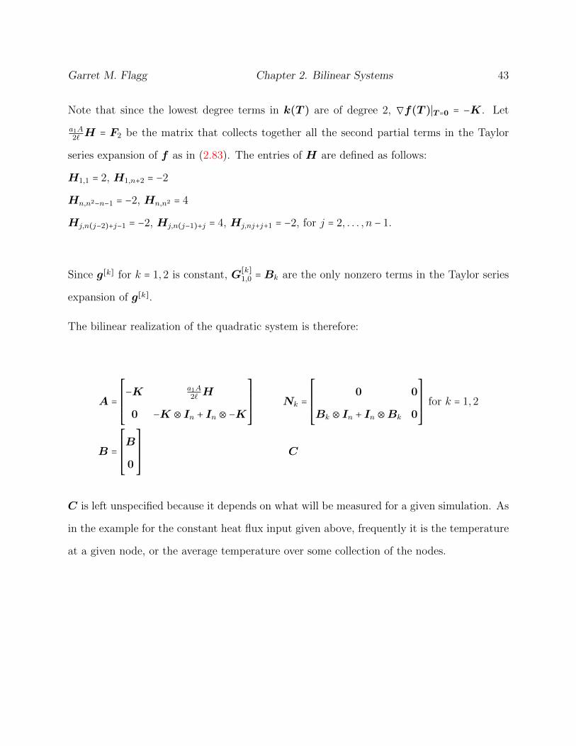
Note that since the lowest degree terms in k(T ) are of degree 2, ∇f(T )∣T=0 = −K. Let
a1A2` H = F2 be the matrix that collects together all the second partial terms in the Taylor
series expansion of f as in (2.83). The entries of H are defined as follows:
H1,1 = 2, H1,n+2 = −2
Hn,n2−n−1 = −2, Hn,n2 = 4
Hj,n(j−2)+j−1 = −2, Hj,n(j−1)+j = 4, Hj,nj+j+1 = −2, for j = 2, . . . , n − 1.
Since g[k] for k = 1,2 is constant, G[k]1,0 =Bk are the only nonzero terms in the Taylor series
expansion of g[k].
The bilinear realization of the quadratic system is therefore:
A =
⎡⎢⎢⎢⎢⎢⎢⎣
−K a1A2` H
0 −K ⊗ In + In ⊗ −K
⎤⎥⎥⎥⎥⎥⎥⎦
Nk =
⎡⎢⎢⎢⎢⎢⎢⎣
0 0
Bk ⊗ In + In ⊗Bk 0
⎤⎥⎥⎥⎥⎥⎥⎦
for k = 1,2
B =
⎡⎢⎢⎢⎢⎢⎢⎣
B
0
⎤⎥⎥⎥⎥⎥⎥⎦
C
C is left unspecified because it depends on what will be measured for a given simulation. As
in the example for the constant heat flux input given above, frequently it is the temperature
at a given node, or the average temperature over some collection of the nodes.

Chapter 3
Model Reduction and Interpolation
Petrov-Galerkin projection and its connection with interpolation theory provides a powerful
theoretical framework for the model reduction of linear dynamical systems. Constructing a
low-order interpolant of the full-order transfer function requires solving shifted linear sys-
tems. Typically the realization for the full-order model is sparse, and so solving the shifted
linear systems can be done at a relatively low computational cost. If an optimal, or asymp-
totically optimal, collection of interpolation points can be determined, the cost of comput-
ing an accurate reduced order model can be dramatically decreased when compared with
grammian-based approaches to model reduction, which are highly accurate but require the
solution of the full-order system grammians in full-matrix arithmetic. For the H2 optimal
approximation of LTI systems, locally optimal reduced order models can be constructed via
interpolation using the Iterative Rational Krylov Algorithm (IRKA) of Gugercin, Antoulas
and Beattie [54]. If further information is known about the pole-distribution of the full-
order transfer function, asymptotically optimal interpolation methods have been proposed
by Druskin et. al in [39, 40, 41] . Recently Flagg, Beattie, and Gugercin showed that it is
possible to construct nearly optimal H∞ LTI system approximations starting from an ap-
44

Garret M. Flagg Chapter 3. Model Reduction and Interpolation 45
proximation that is locally H2 optimal [45, 43]. Thus, interpolation-based model reduction
has a demonstrable track-record of producing computationally efficient algorithms that yield
high fidelity reduced models. For bilinear systems, computing the system grammians in or-
der to apply balanced truncation methods is even more costly than for LTI systems, making
it all the more important to develop an interpolation-based alternative. Interpolation-based
Petrov-Galerkin techniques for bilinear model reduction were first developed in [5], [6],[24],
[78],[34]. In this chapter we will first present the Petrov-Galerkin projection framework for
model reduction generally, and demonstrate how interpolation is accomplished in this frame-
work for LTI systems. We then consider two generalizations of interpolation-based model
reduction to bilinear systems.
3.1 The Petrov-Galerkin model reduction framework
Consider r-dimensional subspaces Vr and Wr of the full order state space. We wish to
construct an approximation x(t) ∈ Vr to the true state x(t) so that
˙x(t) −Ax(t) +Nx(t)u(t) − bu(t) ⊥Wr (3.1)
Let V ,W satisfying W T V = Ir be real n × r matrices whose columns form a basis for Vr
and Wr respectively. The Petrov-Galerkin approximation can be constructed by defining
x(t) = V xr(t) for some xr(t) ∈ Rr and enforcing
W T (V xr(t) −AV xr(t) +NV xru(t) − bu(t)) = 0 (3.2)
Enforcing this condition yields the order r bilinear system

Garret M. Flagg Chapter 3. Model Reduction and Interpolation 46
xr(t) = W TAV xr(t) + W TNV xr(t)u(t) − W Tbu(t)
yr(t) = cV xr(t)(3.3)
In this framework, finding an accurate reduced order model is equivalent to finding accurate
projection subspaces Vr and Wr. Both interpolation and balancing methods are subsumed
under the Petrov-Galerkin framework. In the case of balanced truncation, this is readily
seen by considering the role of the balancing transformation T in the model reduction. After
balancing, ζ has the realization (T −1AT ,T −1NT ,T −1b,cTT ). The projection matrices that
yield a balanced truncation approximation are then given as W = (T Tr )−1, V = Tr, where
Tr is the first r columns of T and (T Tr )−1 is the first r columns of (T T )−1. Interpolation-
based model reduction methods explicitly define the subspaces Vr and Wr based on some
underlying function subspace, such as polynomials, as in the case of Krylov subspaces, or
rational functions as in the case of rational Krylov subspaces. In the next section we will
begin by briefly reviewing interpolation-based model reduction of linear systems, and then
present two natural, but distinct generalizations to bilinear systems.
3.2 Interpolation-based model reduction
LetH(s) ∈ Cp×m be the transfer function of an order n linear system. Given r right-tangential
point-direction pairs (σ1,r1), . . . , (σr,rr) where σj ∈ C and rj ∈ Rm and r left-tangential
point-direction pairs (µ1, `1), . . . , (µr, `r) with µj ∈ C and `j ∈ Rp, the rational tangential
interpolation problem is to construct Hr(s) of order at most r so that

Garret M. Flagg Chapter 3. Model Reduction and Interpolation 47
`TjH(µj) = `TjHr(µj), for j = 1, . . . , r and, (3.4)
H(σj)rj =Hr(σj)rj, for j = 1, . . . , r. (3.5)
Interpolation via projection was first proposed by Skelton et al. [96, 103, 104]. Later,
Grimme [52] showed how to construct a reduced-order interpolant, using a method of Ruhe
[82]. Rational tangential interpolation for MIMO linear dynamical systems as it is presented
here was more recently developed by Gallivan et al. [51]
Theorem 3.1. Let Σ be a linear system with the realization (A,B,C). Given r right-
tangential point-direction pairs (σ1,r1), . . . , (σr,rr) and r left-tangential point-direction pairs
(µ1, `1), . . . , (µr, `r), construct V ,W ∈ Rn×r
so that
Range(V ) = span([(σ1I −A)−1Br1, . . . , (σrI −A)−1Brr]) (3.6)
Range(W ) = span([µ1I −AT )−1CT`1, . . . , (µ1I −A
T )−1C`r]) (3.7)
and W T V = Ir.
Define the reduced-order linear system ζr with the realization
A = W TAV Br = WTB Cr =CV (3.8)
Then ζr satisfies

Garret M. Flagg Chapter 3. Model Reduction and Interpolation 48
`TjH(µj) = `TjHr(µj), for j = 1, . . . , r and, (3.9)
H(σj)rj =Hr(σj)rj, for j = 1, . . . , r. (3.10)
Moreover, if σj = µj for i = 1, . . . r, then
`TjH′(σj)rj = `
TjH
′r(σj)rj, for j = 1, . . . , r. (3.11)
Proof. [51]
Hr(σj)rj =CV (σjIr − A)−1Brrj
=CV (σjIr − A)−1W T (σjIn −A)(σjIn −A)−1Brj
=CV (σjIr − A)−1W T (σjIn −A)V uj, for some uj ∈ Rr
=CV (σjIr − A)−1(σjIr − A)uj
=CV uj
=C(σjIn −A)−1Brj
=H(σj)rj
The statement for the left-tangential vectors can be proved similarly. The statement con-
cerning derivatives is proved as follows

Garret M. Flagg Chapter 3. Model Reduction and Interpolation 49
`TjH′r(σj)rj = `
Tj CV (σjIr − A)−2Brrj
= `Tj CV (σjIr − A)−1W T V (σjIr − A)−1Brrj
= qTj WT V uj, for some uj,qj ∈ Rr
= `Tj C(σjIn −A)−1(σjIn −A)−1Brj
= `TjH′(σj)rj
The construction of the interpolant in Theorem 3.1 underscores the central component of
all projection-based interpolation methods. The basic idea is to project the state onto the
subspace spanned by the system transfer function evaluated at some collection of frequencies,
whenever this makes sense. As we shall see, there are two different ways to push this strategy
forward in the case of bilinear systems. The first approach, which we will call subsystem
interpolation, is to place the interpolation information for a finite number of subsystems in
the span of the projection basis. Recall that for a bilinear system ζ the transfer function
for the kth order homogeneous subsystem in the frequency domain is a k-variate complex-
valued rational function. The total response can be computed by summing over all the
kth-order homogeneous subsystems. Assuming that the contributions to the response from
higher order subsystems is negligible, a good system approximation may be achieved by
matching the low-order subsystems, together with some specified number of their derivatives,
at several different points. The alternative is to enforce matching conditions on the whole
Volterra series. This latter approach is a kind of multipoint interpolation scheme that carries
information from point evaluations at every term in the Volterra series. This approach will be
considered in greater detail after subsystem interpolation, but we note here that the Volterra

Garret M. Flagg Chapter 3. Model Reduction and Interpolation 50
series interpolation approach allows for a construal of the solution of the H2 optimal model
reduction problem for bilinear systems as an interpolation problem, and as such provides
insight into developing other interpolation strategies.
3.3 Subsystem Interpolation
The subsystem interpolation problem is posed in terms of the multimoments of the transfer
functions Hk(s1, . . . , sk).
Definition 3.1 (Multimoments). Let ζ be a bilinear system with realization (A, N1, . . . ,Nm,
B, C). Then for some point (σ1, . . . , σk) ∈ Ck, together with nonnegative integers m1, . . . ,mk,
a multimoment H(m1,...,mk)k (s1, . . . , sk) of the kth order transfer function Hk(s1, . . . , sk) is
defined as
H(m1,...,mk)k (s1, . . . , sk) =C(skI −A)−mkN [Im ⊗ (sk−1I −A)−mk−1](Im ⊗ N)⋯
⋅ [Im ⊗⋯⊗ Im´¹¹¹¹¹¹¹¹¹¹¹¹¹¹¹¹¹¹¹¹¹¹¹¹¹¹¹¹¹¸¹¹¹¹¹¹¹¹¹¹¹¹¹¹¹¹¹¹¹¹¹¹¹¹¹¹¹¹¹¹¶
k−2 times
⊗(s2I −A)−m2](Im ⊗⋯⊗ Im´¹¹¹¹¹¹¹¹¹¹¹¹¹¹¹¹¹¹¹¹¹¹¹¹¹¹¹¹¹¸¹¹¹¹¹¹¹¹¹¹¹¹¹¹¹¹¹¹¹¹¹¹¹¹¹¹¹¹¹¹¶
k−2 times
⊗N) (3.12)
⋅ [Im ⊗⋯⊗ Im´¹¹¹¹¹¹¹¹¹¹¹¹¹¹¹¹¹¹¹¹¹¹¹¹¹¹¹¹¹¸¹¹¹¹¹¹¹¹¹¹¹¹¹¹¹¹¹¹¹¹¹¹¹¹¹¹¹¹¹¹¶
k−1 times
⊗(s1I −A)−m1](Im ⊗⋯⊗ Im´¹¹¹¹¹¹¹¹¹¹¹¹¹¹¹¹¹¹¹¹¹¹¹¹¹¹¹¹¹¸¹¹¹¹¹¹¹¹¹¹¹¹¹¹¹¹¹¹¹¹¹¹¹¹¹¹¹¹¹¹¶
k−1 times
⊗B).
The subsystem interpolation problem was originally introduced by Phillips in [78] for SISO
bilinear systems as a method for matching moments around infinity of the transfer functions
for the kth order homogeneous subsystems. It was later extended to the problem of matching
moments around zero and infinity by Bai and Skoogh [6] , and finally extended to all of Cn by
Breiten and Damm [24]. The subsystem interpolation problem was then further generalized
to the case of multi-input-multi-output systems by Lin, Bao, and Wei [69] for multimoments
around the origin, and requires the construction of block Krylov subspaces. Here we will

Garret M. Flagg Chapter 3. Model Reduction and Interpolation 51
present the most general case of tangential interpolation on the first through the kth order
homogenous subsystems of a bilinear system ζ defined by (2.1).
Theorem 3.2 (Subsystem Interpolation). Let ζ:=(A, N1, . . . ,Nm, B, C) be given, to-
gether with the sequences {σj}kj=1,{γj}kj=1 ⊂ C and vectors cT ∈ Cp and b ∈ Cm Define
bj = oj ⊗ b, and N⊕T = [NT1 , . . . ,N
Tm], where oj is a column of mj−1 ones. Let Kq(M ,x) =
span{x,Mx, . . . ,M q−1x} the standard polynomial Krylov subspace. To construct a reduced
order system ζ that matches all the multimoments H(l1,...,lj)j (σ1, . . . , σj)bj) and
cH(l1,...,lj)
k (γj, . . . , γ1) for j = 1, . . . , k and l1 . . . lj = 1, . . . , q construct the matrices V and W
as follows:
span{V (1)} =Kq((σ1I −A)−1, (σ1I −A)−1Bb) (3.13)
span{W (1)} =Kq((γ1I −A)−∗, (γ1I −A)−∗C∗c∗) (3.14)
span{V (j)} =Kq((σjI −A)−1, (σjI −A)−1N(Im ⊗V (j−1))) for j = 2, . . . , k (3.15)
span{W (j)} =Kq((γjI −A)−T , (γjI −A)−TN⊕T (Im ⊗W (j−1))) for j = 2, . . . , k (3.16)
spanV =span{k
⋃j=1
span{V (j)}} (3.17)
spanW =span{k
⋃j=1
span{W (j)}}. (3.18)
Provided W T = (W TV )−1W T is defined, the system Σr:=( A=W TAV , N=W TNV ,
C=CV , B=W TB) satisfies
H(l1,...,lj)
k (σ1, . . . , σj)bj = H(l1,...,lj)j (σ1, . . . , σj)bj
and
cH(l1,...,lj)j (γj, . . . , γ1) = cH
(l1,...,lj)j (γj, . . . , γ1),

Garret M. Flagg Chapter 3. Model Reduction and Interpolation 52
for j = 1, . . . ,K and l1 . . . lk = 1, . . . , q.
The proof given here reduces to the proof given by Breiten and Damm in [24] for the SISO
result, so I will only include the novel portion.
Proof. Let b=Bb, and c = cC. Fix j ∈ {1, . . . , k}. Define the indexing set Ij =j
⨉`=1
{1,2, . . . , j},
so that each i ∈ Ij is a j-tuple with some combination of the integers 1, . . . , j. Finally, let
Mj =mj−1. In light of equation (2.25),
H(l1,...,lj)(σ1, . . . , σj)bj = ∑i∈Ij
C(σjI −A)−ljNi(j−1)⋯Ni(1)(σ1I −A)−l1 b (3.19)
cH(l1,...,lj)(γ1, . . . , γj) = [c(sjI −A)−1Ni1(j−1)⋯Ni1(1)(s1I −A)−1B, (3.20)
c(γjI −A)−1Ni2(j−1)⋯Ni2(1)(γ1I −A)−1B, . . . , (3.21)
c(γjI −A)−1NiMj (j−1)⋯NiMj (1)(γ1I −A)−1B] (3.22)
Therefore it is sufficient to show that for any i ∈ Ij,
(σjI −A)−ljNi(j−1) . . .Ni(1)(σ1I −A)−l1 b
= V (σjIr − A)−lkNi(j−1) . . . Ni(1)(σ1Ir − A)−l1W T b, and (3.23)
c(γ1I −A)−lkNi(k−1)⋯Ni(1)(γkI −A)−l1
= cV (γ1Ir − A)−ljNi(j−1)⋯Ni(1)(γjIr − A)−l1(W TV )−1W T (3.24)
The vectors
(σjI −A)−ljNi(j−1) . . .Ni(1)(σ1I −A)−l1 b and (c(γ1I −A)−ljNi(j−1)⋯Ni(1)(γjI −A)−l1)T
lie in the range of V andW by construction, so the the proof of equalities 3.23, 3.24 proceeds

Garret M. Flagg Chapter 3. Model Reduction and Interpolation 53
precisely as the proof given by Breiten [24],[25] for the SISO case.
Assuming the subspaces are linearly independent and constructed from a total of ν sequences,
denoted σβ,1, . . . , σβ,N and µβ,1, . . . µβ,ν for β = 1, . . . , ν, the interpolating system ζr will have
dimension r = ν(p1 + 1) + 2ν(p1 + 1)(p2 + 1) + . . . + NνN
∏j=1
(pj + 1), which can clearly grow
large rather quickly. The main advantage of subsystem interpolation is that it does not
depend on convergence of the Volterra series, which in general may be very difficult to
establish. As it stands however, subsystem interpolation is unable to satisfy any known
optimality conditions. Nevertheless, it still makes sense to use this approach if the Volterra
series can be well approximated by truncating the series, as several examples we provide
later demonstrate. This approach also clearly introduces a large number of parameters
that must be determined in order to construct an approximation, and in the absence of a
theory of optimal subsystem interpolation, how to best choose the parameters is anyone’s
guess. In practice, most applications simply assume that interpolation of the first and second
subsystems is sufficient to provide a good characterization of the system, and this mostly
because it is simple.
3.4 Volterra Series Interpolation
Consider the response of a bilinear system ζ to the Heaviside function H(t). The Heaviside
function is defined as the step function
H(t) =
⎧⎪⎪⎪⎪⎨⎪⎪⎪⎪⎩
0 if t < 0
1 if t ≥ 0(3.25)

Garret M. Flagg Chapter 3. Model Reduction and Interpolation 54
For the inputs uk(t) = κH(t) for k = 1, . . . ,m and t > 0 the bilinear system ζ can be written
as
ζ =
⎧⎪⎪⎪⎪⎨⎪⎪⎪⎪⎩
x(t) =Ax(t) + κm
∑k=1Nkx(t) +Bκom
y =Cx(t),
(3.26)
where om is a column of m ones, and therefore the output of ζ is equivalent to a that of the
linear system Σκ with realization (A+κm
∑k=1Nk,B, C). Hence, an accurate approximation of
the system for these inputs corresponds to accurately approximating its linear counterpart.
Let Hκ(s) =C(sI − (A+ κm
∑k=1Nk))
−1B be the transfer function of the system Σκ. Suppose
Σr is approximation to Σκ satisfying some rational tangential interpolation conditions at
points σj and along right and left directions rj and `j, respectively. Does this system satisfy
any interpolation properties interpreted in the context of the underlying bilinear system?
The interpolation conditions for the linear system are given as H(σj)rj =Hr(σj)rj, where
H(σj)rj =C(σjI −A − κm
∑k=1
Nk)−1Brj
=C(I + κ(σjI −A)−1m
∑k=1
Nk)−1(σjI −A)−1Brj. (3.27)
Assuming that ∥(κ(σjI −A)−1m
∑k=1Nk)∥2 < 1, (3.27) can be rewritten as the Neumann series
H(σj)rj =C∞
∑k=0
(κ(σjI −A)−1m
∑k=1
Nk)k(σjI −A)−1Brj (3.28)
=∞
∑k=0
κkHk(σj, . . . , σj)rj, (3.29)
where rj = om ⊗ om ⊗ rj.
Hence, interpolation of the linear system for the Heaviside function corresponds to matching

Garret M. Flagg Chapter 3. Model Reduction and Interpolation 55
the frequency domain Volterra series weighted by κ along the sequences {σj, σj, σj, . . .}.
Moreover, considering the interpretation of the H2 norm as a weighted sum over all possible
combinations of point evaluations in the mirror image of the spectrum of A summed over all
homogeneous subsystems suggests that we may pose a more general multipoint interpolation
problem for which the reduced and full-order systems match on weighted sums of the Volterra
series kernels.
So consider the following interpolation problem. Given two sets of points σ1, σ2, . . . , σr to-
gether with a matrix U ∈ Rr×r and µ1, . . . , µr ∈ C together with a matrix S ∈ Rr×r, fix some
j ∈ {1,2, . . . , r} and define the weighted series
∞
∑k=1
r
∑l1
r
∑l2
⋯r
∑lk−1
ηl1,l2,...,lk−1,j
H(σl1 , σl2 , . . . , σj) <∞
∞
∑k=1
r
∑l1
r
∑l2
⋯r
∑lk−1
ηl1,l2,...,lk−1,j
H(µj, µl2 , . . . , µlk) <∞
where l1, l2, . . . , lk = 1, . . . , r. The weights ηl1,l2,...,lk−1,j
are given in terms of the entries of
U = {ui,j} as
ηl1,l2,...,lk−1,j
= uj,lk−1ulk−1,lk−2⋯ul2,l1 for k ≥ 2 and ηl1 = 1 for l1 = 1, . . . , r. (3.30)
For example, η1,2,3 = u3,2u2,1. Thus, the weights ηl1,l2,...,lk−1,j
are generated by multiplying
sequences of the entries of U together in the combinations determined by the index li.
The weights ηl1,l2,...,lk−1,j
are defined in the same way in terms of the entries of S. Note
that for the interpolation conditions in σj, sk = σj, whereas s1, . . . , sk−1 may take any other
value σ ∈ {σ1, . . . , σr} for all the transfer function evaluations in the series. Analogously,
for the interpolation conditions in µj, s1 = µj, whereas s2 . . . , sk−1 may take any other value
µ ∈ {µ1, . . . , µr} for all the transfer function evaluations in the series. Given this data, the

Garret M. Flagg Chapter 3. Model Reduction and Interpolation 56
goal is to construct a reduced order system ζr ∶=(A, N , b, c) of order r so that for each
j = 1, . . . r
∞
∑k=1
r
∑l1
r
∑l2
⋯r
∑lk−1
ηl1,l2,...,lk−1,j
(Hk(σl1 , σl2 , . . . , σj) − Hk(σl1 , σl2 , . . . , σj)) = 0 (3.31)
and
∞
∑k=1
r
∑l2
r
∑l3
⋯r
∑lk
ηl1,l2,...,lk−1,j
(Hk(σj, σl2 , . . . , σlk) − Hk(σj, σl2 , . . . , σlk)) = 0 (3.32)
The solution to this problem is given as follows.
Theorem 3.3 (Volterra Series Interpolation). Let ζ ∶=(A, N , b, c) be a bilinear system of
order n. Suppose that for some r < n, points σ1, . . . , σr ∈ C and µ1, . . . , µr ∈ C, together with
U ,S ∈ Rr×r are given so that the series
∞
∑k=1
r
∑l1
r
∑l2
⋯r
∑lk−1
ηl1,l2,...,lk−1,j
(σjI −A)−1N(σlk−1I −A)−1N⋯N(σl1I −A)−1b (3.33)
∞
∑k=1
r
∑l1
r
∑l2
⋯r
∑lk−1
ηl1,l2,...,lk−1,j
(µjI −AT )−1NT (µlk−1I −A
T )−1NT⋯NT (µl1I −AT )−1cT
converge for each σj, and µj. Let Λ = diag(σ1, . . . , σr), and M = diag(µ1, . . . , µr) and let V ,
W ∈ Rn×r solve the generalized Sylvester equations
V Λ −AV −NV UT = beT (3.34)
WM −ATW −NTWST = cTeT .

Garret M. Flagg Chapter 3. Model Reduction and Interpolation 57
If W T V ∈ Rr×r is invertible, then the reduced order model ζr of order r defined by
A = (W T V )−1W TAV , N = (W T V )−1W TNV ,
b = (W T V )−1W Tb, c = cV (3.35)
satisfies (3.31) for each σj, µj, j = 1, . . . , r.
Proof. We first show that the jth column of V is equivalent to (3.33). Let V (1) ∈ Rn×r solve
V (1)Λ −AV (1) = beT (3.36)
and for k ≥ 2, let V (k) ∈ Rn×r be the solution to
V (k)Λ −AV (k) =NV (k−1)UT (3.37)
Then V =∞
∑k=0V (k). Let vk,j denote the jth column of V (k). Then v1,j = (σjI −A)−1b, and
in general for k ≥ 2
vk,j = (σjI −A)−1fk−1,j (3.38)
where fk−1,j is the jth column of NV (k−1)U . We show by induction on k that
fk−1,j =r
∑lk−1
r
∑lk−2=1
⋯r
∑l1
ηl1,l2,...,lk−1,j
N(σlk−1I −A)1N(σlk−2I −A)−1N⋯N(σl1I −A)−1b (3.39)
So let k = 2. Then
f1,j =r
∑l1=1
uj,l1Nv
1,l1=
r
∑l1=1
ηl1,jN(σl1I −A)−1b. (3.40)

Garret M. Flagg Chapter 3. Model Reduction and Interpolation 58
Now suppose the statement holds for k > 2. Then
vk,j = (σjI −A)−1fk−1 (3.41)
=r
∑lk−1
r
∑lk−2=1
⋯r
∑l1=1
ηl1,l2,...,lk−1,j
(σjI −A)−1N(σlk−1I −A)−1N⋯(σl1I −A)−1b (3.42)
and therefore
fk,j =r
∑lk
uj,lkNvk,lk (3.43)
=r
∑lk
r
∑lk−1
⋯r
∑l1
uj,lkηl1,l2,...,lk−1,lkN(σlkI −A)−1N⋯N(σl2I −A)−1b (3.44)
=r
∑lk
r
∑lk−1
⋯r
∑l1
ηl1,l2,...,lk−1,lk,jN(σlkI −A)−1N⋯N(σl2I −A)−1b (3.45)
Now define the skew projector P = V (W T V )−1W T . Then
P (V Λ −AV −NV U − beT ) =V (Λ − A − NU − beT ) = 0 (3.46)
Since V is full rank, it follows that Γ = Ir solves the projected Sylvester equation
ΓΛ − AΓ − NΓUT = beT .
By the same construction as above, the jth column of Γ can be represented as
γj =∞
∑k=1
r
∑l1
r
∑l2
⋯r
∑lk−1
ηl1,l2,...,lk−1,j
(σjIr − A)−1N(σlk−1Ir − A)−1N⋯N(σl1Ir − A)−1b

Garret M. Flagg Chapter 3. Model Reduction and Interpolation 59
And therefore
V γj = vj =∞
∑k=1
r
∑l1
r
∑l2
⋯r
∑lk−1
ηl1,l2,...,lk−1,j
V (σjIr − A)−1N(σlk−1Ir − A)−1N⋯N(σl1Ir − A)−1b
(3.47)
=∞
∑k=1
r
∑l1
r
∑l2
⋯r
∑lk−1
ηl1,l2,...,lk−1,j
(σjI −A)−1N(σlk−1I −A)−1N⋯N(σl1I −A)−1b (3.48)
Multiplying equation (3.47) on the left by c gives the desired result in terms of the inter-
polation conditions on σj. For the interpolation conditions in the points µj, observe that
precisely the same construction of the columns of W follows from the proof given above
applied to the equation
WM −ATW −NTWS = cTo
Now P T = W (V TW )−1V T is a skew projection onto the range of W , and
P T (WM −ATW −NTWS − cToT ) (3.49)
= W (V TW )−1((V TW )M − AT (V TW ) − NT (V TW )S − cToT ) (3.50)
= 0 (3.51)
Since W (V TW )−1 is full rank, this implies that Ξ = V TW ∈ Rr×r solves
ΞM − ATΞ − NTΞST − cToT = 0
Again, by the construction given above, the columns ξj ∈ Rr of Ξ for j = 1, . . . , r can be
represented as
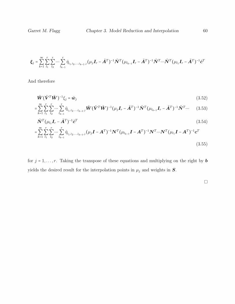
Garret M. Flagg Chapter 3. Model Reduction and Interpolation 60
ξj =∞
∑k=1
r
∑l1
r
∑l2
⋯r
∑lk−1
ηl1,l2,...,lk−1,j
(µjIr − AT )−1NT (µlk−1Ir − A
T )−1NT⋯NT (µl1Ir − AT )−1cT
And therefore
W (V TW )−1ξj = wj (3.52)
=∞
∑k=1
r
∑l1
r
∑l2
⋯r
∑lk−1
ηl1,l2,...,lk−1,j
W (V TW )−1(µjIr − AT )−1NT (µlk−1Ir − A
T )−1NT⋯ (3.53)
NT (µl1Ir − AT )−1cT (3.54)
=∞
∑k=1
r
∑l1
r
∑l2
⋯r
∑lk−1
ηl1,l2,...,lk−1,j
(µjI −AT )−1NT (µlk−1I −A
T )−1NT⋯NT (µl1I −AT )−1cT
(3.55)
for j = 1, . . . , r. Taking the transpose of these equations and multiplying on the right by b
yields the desired result for the interpolation points in µj and weights in S.

Chapter 4
H2 Optimal Model Reduction
In this chapter two different approaches to solving the H2 optimal model reduction problem
are presented. The first approach aims to generalize the structured-orthogonality conditions
first introduced by Gugercin, Beattie, and Antoulas in [54] to the case of bilinear systems.
For LTI systems they showed that certain Hilbert-space orthogonality conditions provided
a unifying framework for all previously derived first-order necessary conditions for the H2
optimal model-reduction problem. The second approach is to directly derive an expression
for the H2 error that can be differentiated with respect to the reduced-order model param-
eters. This approach is carried out in [105] and [20]. For LTI systems both approaches
are equivalent, but in the bilinear case our results show that they are not. Interestingly
enough, the fact that these approaches are not equivalent is grounded in the fact that satis-
fying structured orthogonality conditions would require a subsystem interpolation approach,
whereas the Breiten-Benner [20] and Zhang-Lam [105] conditions require satisfying Volterra
series interpolation conditions. First, consider the structured-orthogonality conditions for
LTI systems summarized in the following theorem.
61

Garret M. Flagg Chapter 4. H2 Optimal Model Reduction 62
Theorem 4.1 (Structured Orthogonality conditions). [54] If Hr has simple poles and sat-
isfies ∥H −Hr∥H2 ≤ ∥H − H(ε)r ∥H2 for any order r system H
(ε)r satisfying ∥Hr − H
(ε)r ∥ ≤ Cε,
then
⟨H −Hr,Hr ⋅H1 +H2⟩H2 = 0 (4.1)
for all real dynamical systems H1, H2 having simple poles at the same locations as Hr.
This inner-product formulation of the optimality conditions can be used to derive the Meier-
Luenberger conditions [71], as well as the Wilson conditions for H2 optimality [101]. In this
sense, they constitute a unifying framework for the H2 model reduction problem in the linear
case, which is the motivation for extending these results to the bilinear case. The Meier-
Luenberger conditions stated here provide a foreshadowing of the type of interpolation-based
necessary conditions we aim to derive for the bilinear case. Here we present them in their
generalized form for MIMO LTI-systems, although they were originally derived for SISO
LTI-systems.
Theorem 4.2 (Meier-Luenberger conditions). [54] Let Σ be an LTI system identified with
its transfer function H(s). Suppose that H(s) =r
∑j=1
1s−λj
cj bTj with bj ∈ Rm, cj ∈ Rp is a
locally H2 optimal approximation to H(s). Then
1.) cTjH(−λj) = cjH(−λj)
2.) H(−λj)bj = H(−λj)bj
3.) cTjH′(−λj)bj = cTj H
′r(−λj)bj, for j = 1, . . . , r.
Recently Gugercin, Beattie, and Antoulas introduced the Iterative Rational Krylov Algo-
rithm (IRKA) as a interpolation-based method for constructing reduced-order models that
are H2 optimal [54]. The algorithm is outlined below.
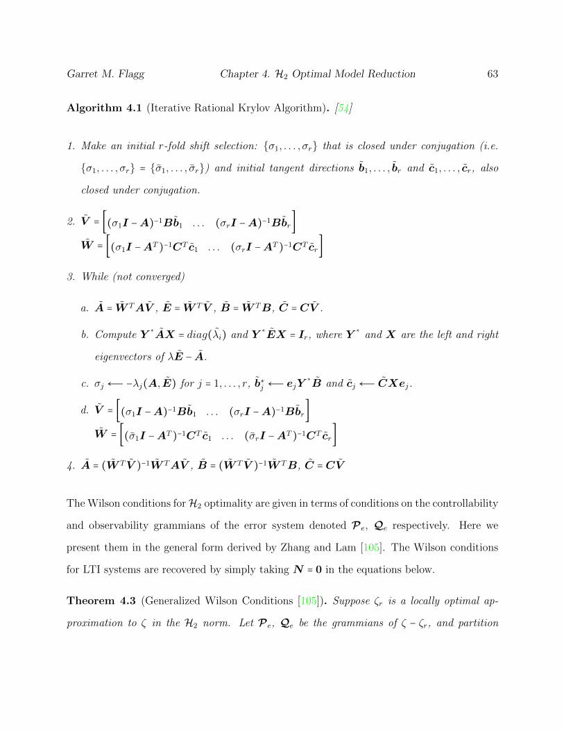
Garret M. Flagg Chapter 4. H2 Optimal Model Reduction 63
Algorithm 4.1 (Iterative Rational Krylov Algorithm). [54]
1. Make an initial r-fold shift selection: {σ1, . . . , σr} that is closed under conjugation (i.e.
{σ1, . . . , σr} = {σ1, . . . , σr}) and initial tangent directions b1, . . . , br and c1, . . . , cr, also
closed under conjugation.
2. V = [(σ1I −A)−1Bb1 . . . (σrI −A)−1Bbr]
W = [(σ1I −AT )−1CT c1 . . . (σrI −AT )−1CT cr]
3. While (not converged)
a. A = W TAV , E = W T V , B = W TB, C =CV .
b. Compute Y∗AX = diag(λi) and Y
∗EX = Ir, where Y
∗and X are the left and right
eigenvectors of λE − A.
c. σj ←Ð −λj(A, E) for j = 1, . . . , r, b∗j ←Ð ejY∗B and cj ←Ð CXej.
d. V = [(σ1I −A)−1Bb1 . . . (σrI −A)−1Bbr]
W = [(σ1I −AT )−1CT c1 . . . (σrI −AT )−1CT cr]
4. A = (W T V )−1W TAV , B = (W T V )−1W TB, C =CV
The Wilson conditions forH2 optimality are given in terms of conditions on the controllability
and observability grammians of the error system denoted Pe, Qe respectively. Here we
present them in the general form derived by Zhang and Lam [105]. The Wilson conditions
for LTI systems are recovered by simply taking N = 0 in the equations below.
Theorem 4.3 (Generalized Wilson Conditions [105]). Suppose ζr is a locally optimal ap-
proximation to ζ in the H2 norm. Let Pe, Qe be the grammians of ζ − ζr, and partition

Garret M. Flagg Chapter 4. H2 Optimal Model Reduction 64
Pe,Qe conformably with the dimensions of A, and A as:
Pe =
⎡⎢⎢⎢⎢⎢⎢⎣
P P0
PT0 Pr
⎤⎥⎥⎥⎥⎥⎥⎦
Qe =
⎡⎢⎢⎢⎢⎢⎢⎣
Q Q0
QT0 Qr
⎤⎥⎥⎥⎥⎥⎥⎦
Then
QT0P0 +QrPr = 0, QrNPr +QT
0NP0 = 0
QT0B +QrB = 0, CPr −CP0 = 0
In order to carry the structured-orthogonality approach forward to the bilinear case, let us
first consider how the analysis will carry forward for SISO bilinear systems. First, define the
Hilbert space
F =∞
⊕k=1
L2((ıR)k).
The inner product on F is defined as the sum of the inner products on each of the com-
ponents, and the elements of F consist of all sequences of functions for which the bilin-
ear H2 norm is finite. In particular, this contains all H2 bilinear systems. Let ⊕H =
(H1(s1),H2(s1, s2),H3(s1, s2, s3), . . . ) be any sequence of proper rational functions of the
form Hk(s1, s2, . . . , sk) =Pn(s1,s2,...,sk)
Qn(s1)Qn(s2)⋯Qn(sk), and assume that ⊕H ∈ F . Let λ1, . . . , λn be
the zeros of Qn, and fix a k ∈ N. Now let the set Jk index the elements of the Cartesian
product Lk =k
⨉i=1
{λ1, . . . , λn}. Lk contains all possible k-tuple combinations of the zeros
of Qn. With each tuple λj ∈ Lk, associate the quantity φk,j as in Definition 2.10. Now
let H{σ1,...,σr} be the subspace of F for which each element ⊕H = (H1(s1), H2(s1, s2), . . . )
satisfies Hk(s1, . . . , sk) = Pr(s1, s2, . . . , sk)/Qr(s1)Qr(s2)⋯Qr(sk), is a strictly proper ra-
tional function and Qr(s`) is a polynomial of degree r with simple zeros at the points

Garret M. Flagg Chapter 4. H2 Optimal Model Reduction 65
σ1, . . . , σr ∈ C. Let Irk index the elements σi of the Cartesian product Sk =k
⨉i=1
{σ1, . . . , σr}.
For any ⊕Hr ∈ H{σ1,...,σr} let φk,i’s be defined for Hk(s1, . . . , sk) also as in Definition 2.10.
Theorem 4.4. If ⊕H⋆ is the optimal approximation to ⊕H out of H{σ1,...,σr}, then for all
k ∈ N and each σi ∈ Sk, ⊕H⋆ satisfies
Hk(−σi(1),−σi(2), . . . ,−σi(k)) = H⋆k (−σi(1),−σi(2), . . . ,−σi(k)) (4.2)
Proof. H{σ1,...,σr} is a closed subspace of F , so by the standard Hilbert projection theorem
⊕H − ⊕H⋆ ⊥ H{σ1,...,σr}. So for any ⊕G ∈ H{σ1,...,σr}
⟨⊕H − ⊕H⋆,⊕G⟩F =
∞
∑k=1
⟨Hk(s1, s2, . . . , sk) − H⋆k (s1, s2, . . . , sk),Gk(s1, s2, . . . , s∞)⟩L2(Rn)
=∞
∑k=1
⎡⎢⎢⎢⎢⎣
∑j∈J n
k
βk,j(H(−σj(1),−σj(2), . . . ,−σj(k)) − H(−σj(1),−σj(2), . . . ,−σj(k)))
⎤⎥⎥⎥⎥⎦
(4.3)
= 0 (4.4)
For each k, there are rk residues βk,j determined by Gk. So expression 4.3 follows from the
pole-residue expansion of Gk, together with an application of the residue calculus in each
variable, as in the proof of Theorem 2.10. Provided the residues βk,j of Gk are chosen small
enough to guarantee convergence, each residue can be chosen to guarantee that the each
term in the sum (4.3) is greater than zero. So to force the sum to 0 over all choices of the
residues of the functions Gk, we must have that
Hk(−σi(1),−σi(2), . . . ,−σi(k)) = H⋆k (−σi(1),−σi(2), . . . ,−σi(k)) (4.5)
Garret M. Flagg Chapter 4. H2 Optimal Model Reduction 66
For a given choice of reduced-order poles, it is possible to construct a sequence of ratio-
nal functions which satisfy the necessary interpolation conditions given by (4.5). However,
in general it is not be possible to find a finite dimensional bilinear realization for this se-
quence, yielding an infinite dimensional solution to the model reduction problem! This is
because there is not a one-to-one correspondence between a minimal bilinear realization and
a sequence of recognizable rational functions. Indeed, it is not possible to carry forward
the structured orthogonality conditions in general, because one can readily show that the
set of r-dimensional bilinear realizations having poles at σ1, . . . , σr is not a closed subspace
of F , although it is certainly a subset of H{σ1,...,σr}. It is worth noting, however, that for
any truncated Volterra series, it is possible to construct a finite dimensional realization of
H⋆(s1, s2, . . . , s∞) which satisfies all of the interpolation conditions.
Now that we have seen that it is not possible to generalize the structured-orthogonality
conditions to the bilinear model reduction problem we return to the more standard approach,
which is to write out the H2 norm of the error system in terms of the realization parameters
A, Nk, B, C, and A, B, Nk C and then differentiate the resulting expression with respect
to the reduced-order model parameters. The next theorem, due to Breiten and Benner [20],
shows how to write the H2 error so that computable necessary conditions can be derived.
Theorem 4.5. [20] Let ζ ∶= (A,N1, . . . ,Nm,B,C) of order n be approximated by a system
ζr ∶= (A, N1, . . . , Nm, B, C) of order r < n. Then
∥ζ − ζr∥2H2
= vec(Ip)T ([C −C]⊗ [C −C])× (4.6)
( −
⎡⎢⎢⎢⎢⎢⎢⎣
A 0
0 Λ
⎤⎥⎥⎥⎥⎥⎥⎦
⊗
⎡⎢⎢⎢⎢⎢⎢⎣
In 0
0 Ir
⎤⎥⎥⎥⎥⎥⎥⎦
−
⎡⎢⎢⎢⎢⎢⎢⎣
In 0
0 Ir
⎤⎥⎥⎥⎥⎥⎥⎦
⊗
⎡⎢⎢⎢⎢⎢⎢⎣
A 0
0 A
⎤⎥⎥⎥⎥⎥⎥⎦
−m
∑k=1
⎡⎢⎢⎢⎢⎢⎢⎣
Nk 0
0 NTk
⎤⎥⎥⎥⎥⎥⎥⎦
⊗
⎡⎢⎢⎢⎢⎢⎢⎣
Nk 0
0 Nk
⎤⎥⎥⎥⎥⎥⎥⎦
)−1
×
(
⎡⎢⎢⎢⎢⎢⎢⎣
B
BT
⎤⎥⎥⎥⎥⎥⎥⎦
⊗
⎡⎢⎢⎢⎢⎢⎢⎣
B
B
⎤⎥⎥⎥⎥⎥⎥⎦
)vec(Im) (4.7)

Garret M. Flagg Chapter 4. H2 Optimal Model Reduction 67
where RΛR−1 is the spectral decomposition of A, and B = BTR−T , C = cR, Nk =
RTNkR−T .
Differentiating this expression with respect to the parameters Λ, B, C, and Nk yields the
following necessary conditions for H2 optimality.
Theorem 4.6 (Necessary conditions for H2 optimality). [20] Suppose ζr is a locally H2
optimal approximation of order r to the full order system ζ. Let RΛR−1 be the spectral
decomposition of A, and let B = BTR−T , C = CR, Nk = RT (N)TR−T for k = 1, . . . ,m.
Then ζr satisfies the following conditions:
vec(Ip)T (eie
Tj ⊗C)( − Λ⊗ In − Ir ⊗A −
m
∑k=1
NTk ⊗Nk)
−1
(BT ⊗B)vec(Im)
= vec(Ip)T (eie
Tj ⊗ C)( − Λ⊗ Ir − Ir ⊗ A −
m
∑k=1
(Nk)T ⊗ Nk)
−1
(BT ⊗ B)vec(Im), (4.8)
vec(Ip)T (C ⊗C)( − Λ⊗ In − Ir ⊗A −
m
∑k=1
NTk ⊗Nk)
−1
(ejeTi ⊗B)vec(Im)
= vec(Ip)T (C ⊗ C)( − Λ⊗ Ir − Ir ⊗ A −
m
∑k=1
(Nk)T ⊗ Nk)
−1
(ejeTi ⊗ B)vec(Im), (4.9)
vec(Ip)T (C ⊗C)( − Λ⊗ In − Ir ⊗A −
m
∑k=1
NTk ⊗Nk)
−1
(eieTi ⊗ In)( − Λ⊗ In − Ir ⊗A −
m
∑k=1
NTk ⊗Nk)
−1
(BT ⊗B)vec(Im)
=vec(Ip)T (C ⊗ C)( − Λ⊗ Ir − Ir ⊗ A −
m
∑k=1
(Nk)T ⊗ Nk)
−1
(eieTi ⊗ In)( − Λ⊗ Ir − Ir ⊗ A −
m
∑k=1
(Nk)T ⊗ Nk)
−1
(BT ⊗ B)vec(Im), and (4.10)

Garret M. Flagg Chapter 4. H2 Optimal Model Reduction 68
vec(Ip)T (C ⊗C)( − Λ⊗ In − Ir ⊗A −
m
∑k=1
NTk ⊗Nk)
−1
(ejeTi ⊗ N)( − Λ⊗ In − Ir ⊗A −
m
∑k=1
NTk ⊗Nk)
−1
(BT ⊗B)vec(Im)
=vec(Ip)T (C ⊗ C)( − Λ⊗ Ir − Ir ⊗ A −
m
∑k=1
(Nk)T ⊗ Nk)
−1
(ejeTi ⊗
¯N)( − Λ⊗ Ir − Ir ⊗ A −m
∑k=1
(Nk)T ⊗ Nk)
−1
(BT ⊗ B)vec(Im) (4.11)
The necessary conditions given in Theorem 4.6 can be used to generalize the Iterative Ra-
tional Krylov Algorithm (IRKA) to the bilinear case. The algorithm below, developed by
Breiten and Benner describes the Bilinear Iterative Rational Krylov Algorithm (B-IRKA).
Algorithm 4.2 (B-IRKA). [20]
Input: A, Nk for k = 1 . . .m, B, C, A, Nk for k = 1, . . . ,m, B, C
Output: Aopt, N optk for k = 1, . . . ,m, Bopt, Copt
1. While: Change in Λ > ε do:
2. RΛR−1 = A, B = BTR−T , C =CR, Nk =RTNTk R
−T for k = 1, . . . ,m.
3. Solve
V (−Λ) −AV −m
∑k=1
NkV NTk =BBT
and
W (−Λ) −AT V −m
∑k=1
NTk W NT
k =CT C
4. V = orth(V ), W = orth(W ).
5. A = (W T V )−1W TAV , Nk = (W T V )−1W TNkV for k = 1, . . . ,m,
B = (W T V )−1W TB, C =CV .

Garret M. Flagg Chapter 4. H2 Optimal Model Reduction 69
6. end while
7. Aopt = A, N optk = Nk for k = 1, . . . ,m, Bopt = B, Copt = C
By setting Nk = 0 for k = 1, . . . ,m, B-IRKA reduces to the Sylvester equation formulation
of IRKA.
We now present an analysis of the necessary conditions of Theorem 4.6 which connects
them with our new multipoint Volterra series interpolation scheme. Our analysis shows that
the Breiten-Benner necessary conditions construed in terms of multipoint Volterra series
interpolation yields rather satisfying generalizations of the Meier-Luenberger conditions, in
the sense that they describe interpolation conditions that can be characterized completely
in terms of the poles and residues of the reduced-order subsystems.
In order to obtain this result, we first prove the following lemma, which clarifies the relation-
ship between the multi-point Volterra series interpolation conditions and the pole residue
expansion of a bilinear system.
Lemma 4.1. Let the SISO bilinear system ζ have the realization A, N , b, c of order n. Let
ζr be a bilinear system of order r < n with realization A, N , b, c. Let RΛR−1 be the spectral
decomposition of A, and let B = BTR−T , C = CR, N = RT (N)TR−T . Moreover, let the
residues φl1,...,lk for k = 1, . . . ,∞ and lk = 1, . . . , r of the transfer functions Hk(s1, . . . , sk)
corresponding to the kth order homogeneous subsystems of ζr be defined as in Definition
2.10. Let V
V (−Λ) −AV −NV NT = bbT
Garret M. Flagg Chapter 4. H2 Optimal Model Reduction 70
Then
c(cV )T =∞
∑k=1
r
∑l1=1
⋯r
∑lk=1
φl1,...,lk
Hk(−λl1 , . . . ,−λk)
(4.12)
Proof. Let U = N , r = b and σj = −λj for j = 1, . . . , r. By applying the construction of the
columns of V given in the proof of Theorem 3.3, we have that
cV (∶, j) =∞
∑k=1
r
∑l1
r
∑l2
⋯r
∑lk−1
ηl1,l2,...,lk−1,j
bl1Hk(−λl1 ,−λl2 , . . . ,−λj)
(4.13)
where recall that ηl1,...,lk−1,j = uj,lk−1ulk−1,lk−2⋯ul2,l1 for k ≥ 2 and ηl1 = 1 for l1 = 1, . . . , r. Now
for each j = 1, . . . , r, observe that by the definition of ηl1,...,lk−1,j, for k ≥ 2
ηl1,...,lk−1,j bl1 = N(j, lk−1)N(lk−1, lk−2)⋯N(l2, l1)bl1 (4.14)
And therefore
∞
∑k=1
r
∑l1
r
∑l2
⋯r
∑lk−1
ηl1,l2,...,lk−1,j
bl1Hk(−λl1 ,−λl2 , . . . ,−λj)
=∞
∑k=1
r
∑l1
r
∑l2
⋯r
∑lk−1N(j, lk−1)N(lk−1, lk−2)⋯N(l2, l1)bl1Hk(−λl1 ,−λl2 , . . . ,−λj)
(4.15)

Garret M. Flagg Chapter 4. H2 Optimal Model Reduction 71
for j = 1, . . . , r. Hence,
(cV )T =
⎡⎢⎢⎢⎢⎢⎢⎢⎢⎢⎢⎢⎢⎢⎢⎢⎢⎣
∞
∑k=1
r
∑l1
r
∑l2
⋯r
∑lk−1N(1, lk−1)N(lk−1, lk−2)⋯N(l2, l1)bl1Hk(−λl1 ,−λl2 , . . . ,−λ1)
∞
∑k=1
r
∑l1
r
∑l2
⋯r
∑lk−1N(2, lk−1)N(lk−1, lk−2)⋯N(l2, l1)bl1Hk(−λl1 ,−λl2 , . . . ,−λ2)
⋮
∞
∑k=1
r
∑l1
r
∑l2
⋯r
∑lk−1N(r, lk−1)N(lk−1, lk−2)⋯N(l2, l1)bl1Hk(−λl1 ,−λl2 , . . . ,−λr)
⎤⎥⎥⎥⎥⎥⎥⎥⎥⎥⎥⎥⎥⎥⎥⎥⎥⎦
Now apply the residue derivation given in (2.72) in the obvious way to the product
[c1 c2 . . . , cr]
⎡⎢⎢⎢⎢⎢⎢⎢⎢⎢⎢⎢⎢⎢⎢⎢⎢⎣
∞
∑k=1
r
∑l1
r
∑l2
⋯r
∑lk−1N(1, lk−1)N(lk−1, lk−2)⋯N(l2, l1)bl1Hk(−λl1 ,−λl2 , . . . ,−λ1)
∞
∑k=1
r
∑l1
r
∑l2
⋯r
∑lk−1N(2, lk−1)N(lk−1, lk−2)⋯N(l2, l1)bl1Hk(−λl1 ,−λl2 , . . . ,−λ2)
⋮
∞
∑k=1
r
∑l1
r
∑l2
⋯r
∑lk−1N(r, lk−1)N(lk−1, lk−2)⋯N(l2, l1)bl1Hk(−λl1 ,−λl2 , . . . ,−λr)
⎤⎥⎥⎥⎥⎥⎥⎥⎥⎥⎥⎥⎥⎥⎥⎥⎥⎦
(4.16)
to obtain
=∞
∑k=1
r
∑l1=1
⋯r
∑lk=1
φl1,...,lk
Hk(−λl1 , . . . ,−λk)
Using Lemma 4.12, we now show that the H2 optimal necessary conditions are equivalent to
multipoint Volterra series interpolation conditions with weights given by the reduced order
residues and interpolation points by the reflection of the poles of the reduced order transfer
functions across the imaginary axis.
Theorem 4.7. Let ζ be a SISO system of order n and suppose that ζ ∈ F . Let ζr =
(A, N , b, c) be an H2 optimal approximation of order r. Then ζr satisfies the following

Garret M. Flagg Chapter 4. H2 Optimal Model Reduction 72
multipoint Volterra series interpolation conditions.
∞
∑k=1
r
∑l1=1
⋯r
∑lk=1
φl1,...,lk
Hk(−λl1 , . . . ,−λk)
=∞
∑k=1
r
∑l1=1
⋯r
∑lk−1=1
φl1,...,lk
Hk(−λl1 , . . . ,−λk), (4.17)
and
∞
∑k=1
r
∑l1=1
⋯r
∑lk=1
φl1,...,lk
(k
∑j=1
∂
∂sjHk(−λl1 , . . . ,−λk))
=∞
∑k=1
r
∑l1=1
⋯r
∑lk=1
φl1,...,lk
(k
∑j=1
∂
∂sjHk(−λl1 , . . . ,−λlk)) (4.18)
where φl1,...,lk
, and λli are the residues and poles of the transfer functions Hk associated with
ζr.
Proof. Let RΛR−1 be the spectral decomposition of A, and let b = bTR−T , c = cR, N =
RTNTR−T . Moreover, suppose that V and W solve
V (−Λ) −AV −NV NT = bbT (4.19)
W (−Λ) −AT V −NTW NT = cT c (4.20)
By applying the vec operator to equations (4.19) and (4.20), we have that
vec(V ) = ( − Λ⊗ In − Ir ⊗A − NT ⊗N)
−1
(bT ⊗ b).
Thus,
(eTj ⊗ c)vec(V ) = cV (∶, j)

Garret M. Flagg Chapter 4. H2 Optimal Model Reduction 73
is equivalent to the left-hand side of necessary condition (4.8). By applying Lemma 4.12 to
both sides of (4.8) gives
∞
∑k=1
r
∑l1=1
⋯r
∑lk=1
φl1,...,lk
Hk(−λl1 , . . . ,−λk)
=∞
∑k=1
r
∑l1=1
⋯r
∑lk−1=1
φl1,...,lk
Hk(−λl1 , . . . ,−λk)
The second equality (4.18) follows from condition (4.10). Simple algebra shows that the right-
hand-side of equality (4.10) is equivalent to the product W (∶, j)T V (∶, j). This is equivalent
to
(∞
∑k=1
r
∑l1=1
⋯r
∑lk−1=1
cl1ηj,lk−1,...,l1c(−λl1In −A)N⋯N(−λlk−1)In −A)−1N(−λjIn −A)−1)⋅
(∞
∑k=1
r
∑r1=1
⋯r
∑rk−1=1
ηr1,...,rk−1,j br1(−λjIn −A)−1N(−λrk−1In −A)−1N⋯N(−λr1In −A)−1b).
(4.21)
Expanding over the first few terms in k is sufficient to establish the general pattern:
W (∶, j)T V (∶, j) = cj bjc(−λjIn −A)−2b +r
∑r1=1
cjηr1,j br1(c(−λjIn −A)−2N(−λr1In −A)−1b
+r
∑l1=1
cl1ηj,l1 bjc(−λl1In −A)−1N(−λjIn −A)−2b)+
+r
∑r1=1
r
∑r2=1
cjηr1,r2,j br1(c(−λjIn −A)−2N(−λr2In −A)−1N(−λr1In −A)−1b
+r
∑l1=1
r
∑l2=1
cl1ηj,l2,l1 bj(c(−λl1In −A)−1N(−λl2In −A)−1N(−λjIn −A)−2b
+r
∑l1=1
r
∑r1=1
cl1ηj,l1ηr1,j br1(c(−λl1In −A)−1N(−λjIn −A)−2N(−λr1In −A)−1b
+ . . . , (4.22)

Garret M. Flagg Chapter 4. H2 Optimal Model Reduction 74
where the weights ηr1,r2,j
, ηj,l2,l1
etc. are defined in (3.30), and the indices in r and l keep
track of the cases where terms on the right are multiplied by terms on the left and vice versa,
respectively. The expansion of the product for the solution of the reduced order matrices
follows similarly. Thus,r
∑j=1W (∶, j)T V (∶, j) gives the desired expression for the derivatives
as:
∞
∑k=1
r
∑l1=1
⋯r
∑lk=1
φl1,...,lk
(k
∑j=1
∂
∂sjHk(−λl1 , . . . ,−λk))
=∞
∑k=1
r
∑l1=1
⋯r
∑lk=1
φl1,...,lk
(k
∑j=1
∂
∂sjHk(−λl1 , . . . ,−λlk)).
Since all the terms j are equal on both sides of equation (4.10), the second result follows.
Enforcing the multipoint interpolation conditions required by Theorem 4.6 or alternatively
Theorem 4.7 requires solving the bilinear Sylvester equations given in Step 3. of B-IRKA.
The direct solution of these equations has O((nr)2) complexity. This means that as r grows
even moderately large, between say 10 and 30, the computational cost will be large per
iteration of B-IRKA. Theorem 4.7 suggests a new and inexpensive, asymptotically optimal
alternative. Instead of matching the entire series and all its first partials at the mirror image
of the reduced order eigenvalues, it is possible to construct approximants ζr that satisfy
the first-order necessary conditions over the first N terms in the series. Moreover, we will
show that this approximation is optimal in an appropriately defined generalization of the H2
norm for bilinear systems. To see this, let us first consider polynomial systems generated by
truncating the Volterra series of a bilinear system.
Definition 4.1. Given a SISO bilinear system ζ with realization (A, N , b, c), define the
polynomial system ζN to be the operator mapping inputs u(t) to ouputs y(t) determined by

Garret M. Flagg Chapter 4. H2 Optimal Model Reduction 75
the following input-output mapping
y(t) =N
∑k=1∫
t
0∫
σ1
0⋯∫
σk−1
0ceA(t−σ1)NeA(σ1−σ2)N
⋯NeA(σk−1−σk)bu(σk)u(σk−1)⋯u(σ1)dσk⋯dσ1
Note that a polynomial system can also be identified with its sequence of transfer functions as
ζN ≡ (H1(s1),H2(s1, s2), . . . ,HN(s1, . . . , sN)) where Hk(s1, . . . , sk) = c(skI−A)−1N⋯N(s1I−
A)−1b, for k = 1, . . .N .
The H2 norm for polynomial systems ζN , denoted HN2 is defined in the obvious way.
Definition 4.2. Let ζN be a polynomial system determined generated by the bilinear system
ζ with realization (A, N , b, c). Then
∥ζN∥HN2=
¿ÁÁÁÀ
N
∑k=1
∞
∫0
⋯
∞
∫0
∣hk(t1, . . . , tk)∣2dtk⋯dt1 (4.23)
Enforcing the multi-point interpolation conditions of Theorem 4.7 on the first N terms is in
fact equivalent to constructing an HN2 optimal approximation of the polynomial system ζN .
Let ζNr be a polynomial reduced order model generated by the bilinear system ζr with
realization (A, N , b, c). We will now derive necessary conditions for HN2 optimality in
terms of the realization parameters of ζr.
From Theorem 2.10,
∥ζN − ζNr ∥2H2
=N
∑k=1
n
∑l1=1
⋅ ⋅ ⋅n
∑lk=1
φl1,...,lk
(Hk(−λl1 , . . . ,−λlk) − Hk(−λl1 , . . . ,−λlk))
−n
∑l1=1
⋅ ⋅ ⋅n
∑lk=1
φl1,...,lk
(Hk(−λl1 , . . . ,−λlk) − Hk(−λl1 , . . . ,−λlk)). (4.24)

Garret M. Flagg Chapter 4. H2 Optimal Model Reduction 76
In terms of the realization parameters of ζ and ζr,
∥ζN − ζNr ∥2 = [c −c](N
∑k=1
Pk)
⎡⎢⎢⎢⎢⎢⎢⎣
c
−c
⎤⎥⎥⎥⎥⎥⎥⎦
, (4.25)
where P0 solves⎡⎢⎢⎢⎢⎢⎢⎣
A 0
0 −Λ
⎤⎥⎥⎥⎥⎥⎥⎦
P0 −
⎡⎢⎢⎢⎢⎢⎢⎣
AT 0
0 −ΛT
⎤⎥⎥⎥⎥⎥⎥⎦
P0 =
⎡⎢⎢⎢⎢⎢⎢⎣
b
b
⎤⎥⎥⎥⎥⎥⎥⎦
[bT bT ]
and for k > 0, Pk solves
⎡⎢⎢⎢⎢⎢⎢⎣
A 0
0 −Λ
⎤⎥⎥⎥⎥⎥⎥⎦
Pk −Pk
⎡⎢⎢⎢⎢⎢⎢⎣
AT 0
0 −ΛT
⎤⎥⎥⎥⎥⎥⎥⎦
=
⎡⎢⎢⎢⎢⎢⎢⎣
N 0
0 N
⎤⎥⎥⎥⎥⎥⎥⎦
Pk−1
⎡⎢⎢⎢⎢⎢⎢⎣
NT 0
0 NT
⎤⎥⎥⎥⎥⎥⎥⎦
This follows as a straightforward application of the construction of the columns of Pk anal-
ogous to the construction given in proof of Theorem 3.3. Applying the vec operator to the
Lyapunov equation for P0 one can write
vec(P0) =⎛
⎝
⎡⎢⎢⎢⎢⎢⎢⎣
In 0
0 Ir
⎤⎥⎥⎥⎥⎥⎥⎦
⊗
⎡⎢⎢⎢⎢⎢⎢⎣
A 0
0 −Λ
⎤⎥⎥⎥⎥⎥⎥⎦
−
⎡⎢⎢⎢⎢⎢⎢⎣
A 0
0 −Λ
⎤⎥⎥⎥⎥⎥⎥⎦
⊗
⎡⎢⎢⎢⎢⎢⎢⎣
In 0
0 Ir
⎤⎥⎥⎥⎥⎥⎥⎦
⎞
⎠
−1 ⎡⎢⎢⎢⎢⎢⎢⎣
b
b
⎤⎥⎥⎥⎥⎥⎥⎦
⊗
⎡⎢⎢⎢⎢⎢⎢⎣
b
b
⎤⎥⎥⎥⎥⎥⎥⎦
(4.26)
and
vec(Pk) =⎛
⎝
⎡⎢⎢⎢⎢⎢⎢⎣
In 0
0 Ir
⎤⎥⎥⎥⎥⎥⎥⎦
⊗
⎡⎢⎢⎢⎢⎢⎢⎣
A 0
0 −Λ
⎤⎥⎥⎥⎥⎥⎥⎦
−
⎡⎢⎢⎢⎢⎢⎢⎣
A 0
0 −Λ
⎤⎥⎥⎥⎥⎥⎥⎦
⊗
⎡⎢⎢⎢⎢⎢⎢⎣
In 0
0 Ir
⎤⎥⎥⎥⎥⎥⎥⎦
⎞
⎠
−1 ⎡⎢⎢⎢⎢⎢⎢⎣
N 0
0 N
⎤⎥⎥⎥⎥⎥⎥⎦
⊗
⎡⎢⎢⎢⎢⎢⎢⎣
N 0
0 N
⎤⎥⎥⎥⎥⎥⎥⎦
vec(Pk−1)
(4.27)
Applying the vec operator to the sum (4.25) and successively substituting the expressions
Garret M. Flagg Chapter 4. H2 Optimal Model Reduction 77
(4.26) and (4.27) into the sum gives
EN =∥ζN − ζNr ∥2
=([c − c]⊗ [c − c])N
∑k=0
⎡⎢⎢⎢⎢⎣
⎛
⎝−
⎡⎢⎢⎢⎢⎢⎢⎣
A 0
0 Λ
⎤⎥⎥⎥⎥⎥⎥⎦
⊗
⎡⎢⎢⎢⎢⎢⎢⎣
In 0
0 Ir
⎤⎥⎥⎥⎥⎥⎥⎦
−
⎡⎢⎢⎢⎢⎢⎢⎣
In 0
0 Ir
⎤⎥⎥⎥⎥⎥⎥⎦
⊗
⎡⎢⎢⎢⎢⎢⎢⎣
A 0
0 Λ
⎤⎥⎥⎥⎥⎥⎥⎦
⎞
⎠
−1
(4.28)
⋅
⎡⎢⎢⎢⎢⎢⎢⎣
N 0
0 N
⎤⎥⎥⎥⎥⎥⎥⎦
⊗
⎡⎢⎢⎢⎢⎢⎢⎣
N 0
0 N
⎤⎥⎥⎥⎥⎥⎥⎦
⎤⎥⎥⎥⎥⎦
k ⎡⎢⎢⎢⎢⎢⎢⎣
b
b
⎤⎥⎥⎥⎥⎥⎥⎦
⊗
⎡⎢⎢⎢⎢⎢⎢⎣
b
b
⎤⎥⎥⎥⎥⎥⎥⎦
The differentiation of EN with respect to the optimization parameters is greatly simplified
by using the following lemma, first derived in [20].
Lemma 4.2 ([20]). Let C(x) ∈ Rp×n, A(y),Gk ∈ Rn×n, and K ∈ Rn×m with
L(y) = −A(y)⊗ I − I ⊗A(y) −m
∑k=1
Gk ⊗Gk
and assume that C and A are differentiable with respect to x, and y. Then
∂
∂x[(vec(Ip))
T (C(x)⊗C(x))L(y)−1(K ⊗K)vec(Im)
= 2(vec(Ip))T (
∂
∂xC(x)⊗C(x))L(y)−1(K ⊗K)vec(Im)
and
∂
∂y[(vec(Ip))
T (C(x)⊗C(x))L(y)−1(B ⊗B)vec(Im)]
= 2(vec(Ip))T (C(x)⊗C(x))L(y)−1(
∂
∂yA(y)⊗ I)L−1(y)(K ⊗K)vec(Im).
Another important tool for analyzing the resulting expressions for the derivative of E is the
permutation matrix

Garret M. Flagg Chapter 4. H2 Optimal Model Reduction 78
M =
⎡⎢⎢⎢⎢⎢⎢⎣
Ir ⊗
⎡⎢⎢⎢⎢⎢⎢⎣
In
0
⎤⎥⎥⎥⎥⎥⎥⎦
Ir ⊗
⎡⎢⎢⎢⎢⎢⎢⎣
0T
Ir
⎤⎥⎥⎥⎥⎥⎥⎦
⎤⎥⎥⎥⎥⎥⎥⎦
(4.29)
first introduced in [20]. Given matrices H ,K ∈ Rr×r and L ∈ Rn×n, the permutation M has
the following property:
MT
⎛⎜⎜⎝
HT ⊗
⎡⎢⎢⎢⎢⎢⎢⎣
L 0
0 K
⎤⎥⎥⎥⎥⎥⎥⎦
⎞⎟⎟⎠
M
= [Ir ⊗ [In0T ] Ir ⊗ [0 Ir]]
⎛⎜⎜⎝
HT ⊗
⎡⎢⎢⎢⎢⎢⎢⎣
L 0
0 K
⎤⎥⎥⎥⎥⎥⎥⎦
⎞⎟⎟⎠
⎡⎢⎢⎢⎢⎢⎢⎣
Ir ⊗
⎡⎢⎢⎢⎢⎢⎢⎣
In
0
⎤⎥⎥⎥⎥⎥⎥⎦
Ir ⊗
⎡⎢⎢⎢⎢⎢⎢⎣
0T
Ir
⎤⎥⎥⎥⎥⎥⎥⎦
⎤⎥⎥⎥⎥⎥⎥⎦
= [Ir ⊗ [In0T ] Ir ⊗ [0 Ir]]
⎡⎢⎢⎢⎢⎢⎢⎣
HT ⊗
⎡⎢⎢⎢⎢⎢⎢⎣
L
0
⎤⎥⎥⎥⎥⎥⎥⎦
HT ⊗
⎡⎢⎢⎢⎢⎢⎢⎣
0T
K
⎤⎥⎥⎥⎥⎥⎥⎦
⎤⎥⎥⎥⎥⎥⎥⎦
=
⎡⎢⎢⎢⎢⎢⎢⎣
HT ⊗L 0
0 HT ⊗K
⎤⎥⎥⎥⎥⎥⎥⎦
Differentiating EN with respect to the parameters Λ, N , b, c and making use of Lemma 4.2
(taking Gk = 0 for k = 1, . . . ,m and K =N in Lemma 4.2) and the permutation M gives
∂EN∂cj
=2([0,−ej]⊗ [c − c])N
∑k=0
⎡⎢⎢⎢⎢⎣
⎛
⎝
⎡⎢⎢⎢⎢⎢⎢⎣
In 0
0 Ir
⎤⎥⎥⎥⎥⎥⎥⎦
⊗
⎡⎢⎢⎢⎢⎢⎢⎣
A 0
0 −Λ
⎤⎥⎥⎥⎥⎥⎥⎦
−
⎡⎢⎢⎢⎢⎢⎢⎣
A 0
0 −Λ
⎤⎥⎥⎥⎥⎥⎥⎦
⊗
⎡⎢⎢⎢⎢⎢⎢⎣
In 0
0 Ir
⎤⎥⎥⎥⎥⎥⎥⎦
⎞
⎠
−1
(4.30)
⋅
⎡⎢⎢⎢⎢⎢⎢⎣
N 0
0 N
⎤⎥⎥⎥⎥⎥⎥⎦
⊗
⎡⎢⎢⎢⎢⎢⎢⎣
N 0
0 N
⎤⎥⎥⎥⎥⎥⎥⎦
⎤⎥⎥⎥⎥⎦
k ⎡⎢⎢⎢⎢⎢⎢⎣
b
b
⎤⎥⎥⎥⎥⎥⎥⎦
⊗
⎡⎢⎢⎢⎢⎢⎢⎣
b
b
⎤⎥⎥⎥⎥⎥⎥⎦

Garret M. Flagg Chapter 4. H2 Optimal Model Reduction 79
=2([0,−ej]⊗ [c − c])N
∑k=0
⎡⎢⎢⎢⎢⎣
⎛
⎝
⎡⎢⎢⎢⎢⎢⎢⎣
In 0
0 Ir
⎤⎥⎥⎥⎥⎥⎥⎦
⊗
⎡⎢⎢⎢⎢⎢⎢⎣
A 0
0 −Λ
⎤⎥⎥⎥⎥⎥⎥⎦
−
⎡⎢⎢⎢⎢⎢⎢⎣
A 0
0 A
⎤⎥⎥⎥⎥⎥⎥⎦
⊗
⎡⎢⎢⎢⎢⎢⎢⎣
In 0
0 Ir
⎤⎥⎥⎥⎥⎥⎥⎦
⎞
⎠
−1
⋅
⎡⎢⎢⎢⎢⎢⎢⎣
N 0
0 N
⎤⎥⎥⎥⎥⎥⎥⎦
⊗
⎡⎢⎢⎢⎢⎢⎢⎣
N 0
0 N
⎤⎥⎥⎥⎥⎥⎥⎦
⎤⎥⎥⎥⎥⎦
k ⎡⎢⎢⎢⎢⎢⎢⎣
b
b
⎤⎥⎥⎥⎥⎥⎥⎦
⊗
⎡⎢⎢⎢⎢⎢⎢⎣
b
b
⎤⎥⎥⎥⎥⎥⎥⎦
=2( − ej ⊗ [c − c])N
∑k=0
⎡⎢⎢⎢⎢⎣
⎛
⎝− Λ⊗
⎡⎢⎢⎢⎢⎢⎢⎣
In 0
0 Ir
⎤⎥⎥⎥⎥⎥⎥⎦
− Ir ⊗
⎡⎢⎢⎢⎢⎢⎢⎣
A 0
0 A
⎤⎥⎥⎥⎥⎥⎥⎦
⎞
⎠
−1
N ⊗
⎡⎢⎢⎢⎢⎢⎢⎣
N 0
0 N
⎤⎥⎥⎥⎥⎥⎥⎦
⎤⎥⎥⎥⎥⎦
k
b⊗
⎡⎢⎢⎢⎢⎢⎢⎣
b
b
⎤⎥⎥⎥⎥⎥⎥⎦
=2( − ej ⊗ [c − c])MTN
∑k=0
⎡⎢⎢⎢⎢⎣
⎛
⎝
⎡⎢⎢⎢⎢⎢⎢⎣
−Λ⊗ In 0
0 −Λ⊗ Ir
⎤⎥⎥⎥⎥⎥⎥⎦
−
⎡⎢⎢⎢⎢⎢⎢⎣
Ir ⊗A 0
0 Ir ⊗ A
⎤⎥⎥⎥⎥⎥⎥⎦
⎞
⎠
−1
⋅
⎡⎢⎢⎢⎢⎢⎢⎣
N ⊗N 0
0 N ⊗ N
⎤⎥⎥⎥⎥⎥⎥⎦
⎤⎥⎥⎥⎥⎦
k
M⎛
⎝b⊗
⎡⎢⎢⎢⎢⎢⎢⎣
b
b
⎤⎥⎥⎥⎥⎥⎥⎦
⎞
⎠
=(−2ej ⊗ c)N
∑k=0
[( − Λ⊗ In − Ir ⊗A)
−1
N ⊗N]
k
(b⊗ b)
+ 2(ej ⊗ c)N
∑k=0
[( − Λ⊗ Ir − Ir ⊗ A)
−1
N ⊗ N]
k
(b⊗ b) (4.31)
∂EN
∂λj=([c − c]⊗ [c − c])
N
∑k=0
k−1
∑j=0
⎡⎢⎢⎢⎢⎣
⎛
⎝−
⎡⎢⎢⎢⎢⎢⎢⎣
A 0
0 Λ
⎤⎥⎥⎥⎥⎥⎥⎦
⊗
⎡⎢⎢⎢⎢⎢⎢⎣
In 0
0 Ir
⎤⎥⎥⎥⎥⎥⎥⎦
−
⎡⎢⎢⎢⎢⎢⎢⎣
In 0
0 Ir
⎤⎥⎥⎥⎥⎥⎥⎦
⊗
⎡⎢⎢⎢⎢⎢⎢⎣
A 0
0 Λ
⎤⎥⎥⎥⎥⎥⎥⎦
⎞
⎠
−1
⋅
⎡⎢⎢⎢⎢⎢⎢⎣
N 0
0 N
⎤⎥⎥⎥⎥⎥⎥⎦
⊗
⎡⎢⎢⎢⎢⎢⎢⎣
N 0
0 N
⎤⎥⎥⎥⎥⎥⎥⎦
⎤⎥⎥⎥⎥⎦
j⎛
⎝−
⎡⎢⎢⎢⎢⎢⎢⎣
A 0
0 Λ
⎤⎥⎥⎥⎥⎥⎥⎦
⊗
⎡⎢⎢⎢⎢⎢⎢⎣
In 0
0 Ir
⎤⎥⎥⎥⎥⎥⎥⎦
−
⎡⎢⎢⎢⎢⎢⎢⎣
In 0
0 Ir
⎤⎥⎥⎥⎥⎥⎥⎦
⊗
⎡⎢⎢⎢⎢⎢⎢⎣
A 0
0 Λ
⎤⎥⎥⎥⎥⎥⎥⎦
⎞
⎠
−1
(
⎡⎢⎢⎢⎢⎢⎢⎣
0 0
0 eieTi
⎤⎥⎥⎥⎥⎥⎥⎦
⊗
⎡⎢⎢⎢⎢⎢⎢⎣
In 0
0 Ir
⎤⎥⎥⎥⎥⎥⎥⎦
)⎛
⎝−
⎡⎢⎢⎢⎢⎢⎢⎣
A 0
0 Λ
⎤⎥⎥⎥⎥⎥⎥⎦
⊗
⎡⎢⎢⎢⎢⎢⎢⎣
In 0
0 Ir
⎤⎥⎥⎥⎥⎥⎥⎦
−
⎡⎢⎢⎢⎢⎢⎢⎣
In 0
0 Ir
⎤⎥⎥⎥⎥⎥⎥⎦
⊗
⎡⎢⎢⎢⎢⎢⎢⎣
A 0
0 Λ
⎤⎥⎥⎥⎥⎥⎥⎦
⎞
⎠
−1

Garret M. Flagg Chapter 4. H2 Optimal Model Reduction 80
⎡⎢⎢⎢⎢⎣
⎛
⎝−
⎡⎢⎢⎢⎢⎢⎢⎣
A 0
0 Λ
⎤⎥⎥⎥⎥⎥⎥⎦
⊗
⎡⎢⎢⎢⎢⎢⎢⎣
In 0
0 Ir
⎤⎥⎥⎥⎥⎥⎥⎦
−
⎡⎢⎢⎢⎢⎢⎢⎣
In 0
0 Ir
⎤⎥⎥⎥⎥⎥⎥⎦
⊗
⎡⎢⎢⎢⎢⎢⎢⎣
A 0
0 Λ
⎤⎥⎥⎥⎥⎥⎥⎦
⎞
⎠
−1
⋅
⎡⎢⎢⎢⎢⎢⎢⎣
N 0
0 N
⎤⎥⎥⎥⎥⎥⎥⎦
⊗
⎡⎢⎢⎢⎢⎢⎢⎣
N 0
0 N
⎤⎥⎥⎥⎥⎥⎥⎦
⎤⎥⎥⎥⎥⎦
k−j−1 ⎡⎢⎢⎢⎢⎢⎢⎣
b
b
⎤⎥⎥⎥⎥⎥⎥⎦
⊗
⎡⎢⎢⎢⎢⎢⎢⎣
b
b
⎤⎥⎥⎥⎥⎥⎥⎦
=([c − c]⊗ [c − c])N
∑k=0
k−1
∑j=0
⎡⎢⎢⎢⎢⎣
⎛
⎝−
⎡⎢⎢⎢⎢⎢⎢⎣
A 0
0 Λ
⎤⎥⎥⎥⎥⎥⎥⎦
⊗
⎡⎢⎢⎢⎢⎢⎢⎣
In 0
0 Ir
⎤⎥⎥⎥⎥⎥⎥⎦
−
⎡⎢⎢⎢⎢⎢⎢⎣
In 0
0 Ir
⎤⎥⎥⎥⎥⎥⎥⎦
⊗
⎡⎢⎢⎢⎢⎢⎢⎣
A 0
0 A
⎤⎥⎥⎥⎥⎥⎥⎦
⎞
⎠
−1
⋅
⎡⎢⎢⎢⎢⎢⎢⎣
N 0
0 N
⎤⎥⎥⎥⎥⎥⎥⎦
⊗
⎡⎢⎢⎢⎢⎢⎢⎣
N 0
0 N
⎤⎥⎥⎥⎥⎥⎥⎦
⎤⎥⎥⎥⎥⎦
j⎛
⎝−
⎡⎢⎢⎢⎢⎢⎢⎣
A 0
0 Λ
⎤⎥⎥⎥⎥⎥⎥⎦
⊗
⎡⎢⎢⎢⎢⎢⎢⎣
In 0
0 Ir
⎤⎥⎥⎥⎥⎥⎥⎦
−
⎡⎢⎢⎢⎢⎢⎢⎣
In 0
0 Ir
⎤⎥⎥⎥⎥⎥⎥⎦
⊗
⎡⎢⎢⎢⎢⎢⎢⎣
A 0
0 A
⎤⎥⎥⎥⎥⎥⎥⎦
⎞
⎠
−1
(
⎡⎢⎢⎢⎢⎢⎢⎣
0 0
0 eieTi
⎤⎥⎥⎥⎥⎥⎥⎦
⊗
⎡⎢⎢⎢⎢⎢⎢⎣
In 0
0 Ir
⎤⎥⎥⎥⎥⎥⎥⎦
)⎛
⎝−
⎡⎢⎢⎢⎢⎢⎢⎣
A 0
0 Λ
⎤⎥⎥⎥⎥⎥⎥⎦
⊗
⎡⎢⎢⎢⎢⎢⎢⎣
In 0
0 Ir
⎤⎥⎥⎥⎥⎥⎥⎦
−
⎡⎢⎢⎢⎢⎢⎢⎣
In 0
0 Ir
⎤⎥⎥⎥⎥⎥⎥⎦
⊗
⎡⎢⎢⎢⎢⎢⎢⎣
A 0
0 A
⎤⎥⎥⎥⎥⎥⎥⎦
⎞
⎠
−1
⎡⎢⎢⎢⎢⎣
⎛
⎝−
⎡⎢⎢⎢⎢⎢⎢⎣
A 0
0 Λ
⎤⎥⎥⎥⎥⎥⎥⎦
⊗
⎡⎢⎢⎢⎢⎢⎢⎣
In 0
0 Ir
⎤⎥⎥⎥⎥⎥⎥⎦
−
⎡⎢⎢⎢⎢⎢⎢⎣
In 0
0 Ir
⎤⎥⎥⎥⎥⎥⎥⎦
⊗
⎡⎢⎢⎢⎢⎢⎢⎣
A 0
0 A
⎤⎥⎥⎥⎥⎥⎥⎦
⎞
⎠
−1
⋅
⎡⎢⎢⎢⎢⎢⎢⎣
N 0
0 N
⎤⎥⎥⎥⎥⎥⎥⎦
⊗
⎡⎢⎢⎢⎢⎢⎢⎣
N 0
0 N
⎤⎥⎥⎥⎥⎥⎥⎦
⎤⎥⎥⎥⎥⎦
k−j−1 ⎡⎢⎢⎢⎢⎢⎢⎣
b
b
⎤⎥⎥⎥⎥⎥⎥⎦
⊗
⎡⎢⎢⎢⎢⎢⎢⎣
b
b
⎤⎥⎥⎥⎥⎥⎥⎦
=( − c⊗ [c − c])N
∑k=0
k−1
∑j=0
⎡⎢⎢⎢⎢⎣
⎛
⎝− Λ⊗
⎡⎢⎢⎢⎢⎢⎢⎣
In 0
0 Ir
⎤⎥⎥⎥⎥⎥⎥⎦
− Ir ⊗
⎡⎢⎢⎢⎢⎢⎢⎣
A 0
0 A
⎤⎥⎥⎥⎥⎥⎥⎦
⎞
⎠
−1
N ⊗
⎡⎢⎢⎢⎢⎢⎢⎣
N 0
0 N
⎤⎥⎥⎥⎥⎥⎥⎦
⎤⎥⎥⎥⎥⎦
j
⋅⎛
⎝− Λ⊗
⎡⎢⎢⎢⎢⎢⎢⎣
In 0
0 Ir
⎤⎥⎥⎥⎥⎥⎥⎦
− Ir ⊗
⎡⎢⎢⎢⎢⎢⎢⎣
A 0
0 A
⎤⎥⎥⎥⎥⎥⎥⎦
⎞
⎠
−1
(eieTi ⊗
⎡⎢⎢⎢⎢⎢⎢⎣
In 0
0 Ir
⎤⎥⎥⎥⎥⎥⎥⎦
)
⎛
⎝− Λ⊗
⎡⎢⎢⎢⎢⎢⎢⎣
In 0
0 Ir
⎤⎥⎥⎥⎥⎥⎥⎦
− Ir ⊗
⎡⎢⎢⎢⎢⎢⎢⎣
A 0
0 A
⎤⎥⎥⎥⎥⎥⎥⎦
⎞
⎠
−1⎡⎢⎢⎢⎢⎣
⎛
⎝− Λ⊗
⎡⎢⎢⎢⎢⎢⎢⎣
In 0
0 Ir
⎤⎥⎥⎥⎥⎥⎥⎦
− Ir ⊗
⎡⎢⎢⎢⎢⎢⎢⎣
A 0
0 A
⎤⎥⎥⎥⎥⎥⎥⎦
⎞
⎠
−1
⋅ N ⊗
⎡⎢⎢⎢⎢⎢⎢⎣
N 0
0 N
⎤⎥⎥⎥⎥⎥⎥⎦
⎤⎥⎥⎥⎥⎦
k−j−1
(b⊗
⎡⎢⎢⎢⎢⎢⎢⎣
b
b
⎤⎥⎥⎥⎥⎥⎥⎦
)
=( − c⊗ [c − c])MTN
∑k=0
k−1
∑j=0
⎡⎢⎢⎢⎢⎣
⎛
⎝
⎡⎢⎢⎢⎢⎢⎢⎣
−Λ⊗ In 0
0 −Λ⊗ Ir
⎤⎥⎥⎥⎥⎥⎥⎦
−
⎡⎢⎢⎢⎢⎢⎢⎣
Ir ⊗A 0
0 Ir ⊗ A
⎤⎥⎥⎥⎥⎥⎥⎦
⎞
⎠
−1

Garret M. Flagg Chapter 4. H2 Optimal Model Reduction 81
⋅
⎡⎢⎢⎢⎢⎢⎢⎣
N ⊗N 0
0 N ⊗ N
⎤⎥⎥⎥⎥⎥⎥⎦
⎤⎥⎥⎥⎥⎦
j⎛
⎝
⎡⎢⎢⎢⎢⎢⎢⎣
−Λ⊗ In 0
0 −Λ⊗ Ir
⎤⎥⎥⎥⎥⎥⎥⎦
−
⎡⎢⎢⎢⎢⎢⎢⎣
Ir ⊗A 0
0 Ir ⊗ A
⎤⎥⎥⎥⎥⎥⎥⎦
⎞
⎠
−1
(
⎡⎢⎢⎢⎢⎢⎢⎣
eieTi ⊗ In 0
0 eieTi ⊗ Ir
⎤⎥⎥⎥⎥⎥⎥⎦
)⎛
⎝
⎡⎢⎢⎢⎢⎢⎢⎣
−Λ⊗ In 0
0 −Λ⊗ Ir
⎤⎥⎥⎥⎥⎥⎥⎦
−
⎡⎢⎢⎢⎢⎢⎢⎣
Ir ⊗A 0
0 Ir ⊗ A
⎤⎥⎥⎥⎥⎥⎥⎦
⎞
⎠
−1
⎡⎢⎢⎢⎢⎣
⎛
⎝
⎡⎢⎢⎢⎢⎢⎢⎣
−Λ⊗ In 0
0 −Λ⊗ Ir
⎤⎥⎥⎥⎥⎥⎥⎦
−
⎡⎢⎢⎢⎢⎢⎢⎣
Ir ⊗A 0
0 Ir ⊗ A
⎤⎥⎥⎥⎥⎥⎥⎦
⎞
⎠
−1 ⎡⎢⎢⎢⎢⎢⎢⎣
N ⊗N 0
0 N ⊗ N
⎤⎥⎥⎥⎥⎥⎥⎦
⎞
⎠
⎤⎥⎥⎥⎥⎦
k−j−1 ⎡⎢⎢⎢⎢⎢⎢⎣
b⊗ b
b⊗ b
⎤⎥⎥⎥⎥⎥⎥⎦
= − (c⊗ c)N
∑k=1
k−1
∑j=0
[(−Λ⊗ In − Ir ⊗A)−1N ⊗N]
j
(−Λ⊗ In − Ir ⊗A)−1(eieTi ⊗ In)
(−Λ⊗ In − Ir ⊗A)−1[(−Λ⊗ In − Ir ⊗A)−1N ⊗N]
k−j−1
b⊗ b
+ (c⊗ c)N
∑k=1
k−1
∑j=0
[(−Λ⊗ Ir − Ir ⊗ A)−1N ⊗ N]
j
(−Λ⊗ Ir − Ir ⊗ A)−1(eieTi ⊗ Ir)
(−Λ⊗ In − Ir ⊗ A)−1[(−Λ⊗ Ir − Ir ⊗ A)−1N ⊗ N]
k−j−1
b⊗ b (4.32)
Simplifying these bloated expressions for the other derivatives requires exactly the same
kinds of steps as in simplifying the derivative of E with respect to the parameters in c and
λi, so we omit the derivations here. The resulting expressions are
∂EN
∂bj=(−2c⊗ c)
N
∑k=0
[( − Λ⊗ In − Ir ⊗A)
−1
N ⊗N]
k
(ej ⊗ b)
+ 2(c⊗ c)N
∑k=0
[( − Λ⊗ Ir − Ir ⊗ A)
−1
N ⊗ N]
k
(ej ⊗ b) (4.33)
Garret M. Flagg Chapter 4. H2 Optimal Model Reduction 82
∂EN
∂Ni,j
= − 2(c⊗ c)N
∑k=1
k
∑j=1
[(−Λ⊗ In − Ir ⊗A)−1N ⊗N]
j−1
(−Λ⊗ In − Ir ⊗A)−1(eieTj ⊗ In)
[(−Λ⊗ In − Ir ⊗A)−1N ⊗N]
k−j
(−Λ⊗ In − Ir ⊗A)−1b⊗ b
+ 2(c⊗ c)N
∑k=1
k
∑j=1
[(−Λ⊗ Ir − Ir ⊗ A)−1N ⊗ N]
j−1
(−Λ⊗ Ir − Ir ⊗ A)−1(eieTj ⊗ Ir)
[(−Λ⊗ Ir − Ir ⊗ A)−1N ⊗ N]
k−j
(−Λ⊗ Ir − Ir ⊗ A)−1b⊗ b (4.34)
Remark 4.1. This derivation of the HN2 optimal necessary conditions for the approximation
of a degree N polynomial system ζN is essentially the partial sums version of the first order
necessary conditions for H2 optimality applied to the bilinear system ζ, where limN→∞
ζN = ζ.
That is, taking N →∞ gives the necessary conditions of Theorem 4.6.
The following theorem retranslates the necessary conditions gained from setting expressions
(4.31)-(4.34) to zero into multipoint interpolation conditions on the truncated Volterra series.
Theorem 4.8. Let ζ = (A,N ,b,c) be an order n bilinear system and ζN be the polynomial
system determined by ζ. Let ζr = (A, N , b, c) be a bilinear system of order r, and define ζNr
as the polynomial system determined by ζr. Suppose that ζNr is an H2 optimal approximation
to ζN . Then ζNr satisfies
N
∑k=1
r
∑l1=1
⋯r
∑lk=1
φl1,...,lk
Hk(−λl1 , . . . ,−λk)
=N
∑k=1
r
∑l1=1
⋯r
∑lk−1=1
φl1,...,lk
Hk(−λl1 , . . . ,−λk), (4.35)
Garret M. Flagg Chapter 4. H2 Optimal Model Reduction 83
and
N
∑k=1
r
∑l1=1
⋯r
∑lk=1
φl1,...,lk
(k
∑j=1
∂
∂sjHk(−λl1 , . . . ,−λk))
=N
∑k=1
r
∑l1=1
⋯r
∑lk=1
φl1,...,lk
(k
∑j=1
∂
∂sjHk(−λl1 , . . . ,−λlk)) (4.36)
where φl1,...,lk
, and λli are the residues and poles of Hk associated with ζNr .
Proof. Setting expression (4.31) to zero requires that
ej ⊗ cN
∑k=0
[( − Λ⊗ In − Ir ⊗A)
−1
N ⊗N]
k
(b⊗ b)
=ej ⊗ cN
∑k=0
[( − Λ⊗ Ir − Ir ⊗ A)
−1
N ⊗ N]
k
(b⊗ b) (4.37)
The left-hand side of (4.37), is equivalent to the product cN
∑k=0Vk(∶, j), where V0 solves
V0(−Λ) −V0A = bbT
and for k > 1, Vk solves
Vk(−Λ) −VkA =NVk−1NT (4.38)
Thus, we may apply Lemma 4.12, noting that by the proof of the lemma, the result also
applies for any of the partial sumsN
∑k=0Vk(∶, j) which correspond to the first N terms in the
solution of the generalized Sylvester equation
V (−Λ) − V A −NV NT = bb.T

Garret M. Flagg Chapter 4. H2 Optimal Model Reduction 84
Thus, we conclude that
N
∑k=1
r
∑l1=1
⋯r
∑lk=1
φl1,...,lk
Hk(−λl1 , . . . ,−λlk) (4.39)
=N
∑k=1
r
∑l1=1
⋯r
∑lk=1
φl1,...,lk
Hk(−λl1 , . . . ,−λlk) (4.40)
Now consider (4.32). Setting this expression equal to zero requires that
(c⊗ c)N
∑k=1
k−1
∑j=0
[(−Λ⊗ In − Ir ⊗A)−1N ⊗N]
j
(−Λ⊗ In − Ir ⊗A)−1(eieTi ⊗ In)
(−Λ⊗ In − Ir ⊗A)−1[(−Λ⊗ In − Ir ⊗A)−1N ⊗N]
k−j−1
b⊗ b
=(c⊗ c)N
∑k=1
k−1
∑j=0
[(−Λ⊗ Ir − Ir ⊗ A)−1N ⊗ N]
j
(−Λ⊗ Ir − Ir ⊗ A)−1(eieTi ⊗ Ir)
(−Λ⊗ In − Ir ⊗ A)−1[(−Λ⊗ Ir − Ir ⊗ A)−1N ⊗ N]
k−j−1
b⊗ b (4.41)
Fixing the summation index k, consider the summation
k−1
∑j=0
(c⊗ c)[(−Λ⊗ In − Ir ⊗A)−1N ⊗N]
j
(−Λ⊗ In − Ir ⊗A)−1(eieTi ⊗ In)
(−Λ⊗ In − Ir ⊗A)−1[(−Λ⊗ In − Ir ⊗A)−1N ⊗N]
k−j−1
b⊗ b (4.42)
The expression
(c⊗ c)[(−Λ⊗ In − Ir ⊗A)−1N ⊗N]
j
(−Λ⊗ In − Ir ⊗A)−1
corresponds to vec(Wj)T , where for j > 0, Wj solves
Wj(−Λ) −ATWj −NTWj−1N = cT c

Garret M. Flagg Chapter 4. H2 Optimal Model Reduction 85
and when j = 0,
Wj(−Λ) −ATWj = cT c
Similarly, the expression
(−Λ⊗ In − Ir ⊗A)−1[(−Λ⊗ In − Ir ⊗A)−1N ⊗N]
k−j−1
b⊗ b
corresponds to vec(Vk−j−1), where Vk−j−1 solves the dual Sylvester equations. Therefore the
jth term in the sum (4.42) is equivalent to the product
(Wj(∶, i))TVk−j−1(∶, i)
We can therefore write
(c⊗ c)N
∑k=1
k−1
∑j=0
[(−Λ⊗ In − Ir ⊗A)−1N ⊗N]
j
(−Λ⊗ In − Ir ⊗A)−1(eieTi ⊗ In)
(−Λ⊗ In − Ir ⊗A)−1[(−Λ⊗ In − Ir ⊗A)−1N ⊗N]
k−j−1
b⊗ b (4.43)
=N
∑k=1
k−1
∑j=0
(Wj(∶, i))TVk−j(∶, i)) = (
N
∑k=1
(Wj(∶, i))T )(
N
∑k=1
Vk(∶, i)) (4.44)
The equality
N
∑k=1
r
∑l1=1
⋯r
∑lk=1
φl1,...,lk
(k
∑j=1
∂
∂sjHk(−λl1 , . . . ,−λk))
=N
∑k=1
r
∑l1=1
⋯r
∑lk=1
φl1,...,lk
(k
∑j=1
∂
∂sjHk(−λl1 , . . . ,−λlk)) (4.45)
now follows by exactly the same argument as in the proof of the derivative result for Theorem
4.17, where the only difference is the that the series terminates after N terms.

Garret M. Flagg Chapter 4. H2 Optimal Model Reduction 86
The multipoint truncated-Volterra series interpolation conditions derived in Theorem 4.8 can
be enforced via the following algorithm, which we will call truncated B-IRKA or TB-IRKA.
Algorithm 4.3 (TB-IRKA). Input: A, N , b, c, A, N , b, c, N
Output: Aopt, N opt, bopt, copt
1. While: Change in Λ > 0 do:
2. RΛR−1 = A, b = bTR−T , c = cR, N =RTNTR−T
3. Solve
V1(−Λ) −AV1 = bbT
W1(−Λ) −ATW1 = cT cT
4. For j = 2, . . . ,N , solve
Vj(−Λ) −AVj =NVj−1NT
Wj(−Λ) −ATWj =NTWj−1N
T
5. V = (N
∑j=0Vj), W = (
N
∑k=0Wj).
6. A = (W T V )−1W TAV , N = (W T V )−1W TNV , b = (W T V )−1W Tb, c = cV .
7. end while
8. Aopt = A, N opt = N , bopt = b, copt = c
Upon convergence, the reduced order model ζr = (A, N , b, c) satisfies the interpolation

Garret M. Flagg Chapter 4. H2 Optimal Model Reduction 87
conditions of Theorem 4.8. This follows from the fact that V and W solve
V (−Λ) −AV −NN
∑j=0
VjNT = bbT (4.46)
W (−Λ) −ATW −NTN
∑j=0
WjN = cT c (4.47)
and as we have seen the reduced matrices A, N , b, cconstructed by projecting onto V and
along W satisfy the multipoint interpolation conditions on the first N terms.
The advantage of TB-IRKA is that it requires only 2Nr sparse linear solves per iteration to
exactly solve the ordinary Sylvester equations given in steps 3. and 4. of TB-IRKA. The
computational complexity of each linear solve is therefore on the order of n2, rather than
(rn)2. Thus as r grows, the total cost due to the reduced dimension r remains negligible,
making the cost of TB-IRKA comparable to IRKA, its linear counterpart . Moreover, we
have observed that in order for bilinear systems to stay in F , the magnitude of the terms in
the Volterra series decays very rapidly, so that comparable results to the algorithm B-IRKA
may be obtained by keeping only the first 3 or 4 terms in the series. The numerical examples
below demonstrate the results of using this approach.
A bilinear model of the Fokker-Planck equations
The following example is an application from stochastic control that was first introduced
by Hartmann et. al in [29] and later used as a test case for B-IRKA in [20]. Consider a
Brownian particle confined by a double-well potential W (x) = (x2−1)2. Assume the particle
is initially in the left well, and is dragged to the right well. The particle’s motion can be

Garret M. Flagg Chapter 4. H2 Optimal Model Reduction 88
described by the stochastic differential equation
dXt = −∇V (Xt, t)dt +√
2σdWt,
with σ = 2/3 and V (x,u) = W (x, t) + Φ(x,ut) = W (x) − xu − x. As an alternative to
these equations it is noted in [29] that one can instead determine the underlying probability
distribution function
ρ(x, t)dx = P [Xt ∈ [x,x + dx)]
which is described by the Fokker-Planck equation
∂ρ
∂t= σ∆ρ +∇ ⋅ (ρ∇V ), (x, t) ∈ (a, b) × (0, T ],
0 = σ∇ρ + ρ∇B, (x, t) ∈ {a, b} × [0, T ],
ρ0 = ρ, (x, t) ∈ (a, b) × 0
A finite-difference discretization of the Fokker-Planck equations consisting of 500 nodes in the
interval [−2,2] leads to a SISO bilinear system, where the output matrix c is a discretization
of the (set-theoretic) characteristic function of the interval [0.95,1.05]. Figure 4.1 compares
the relative H2 error in the reduced order models computed from B-IRKA and TB-IRKA
after truncating at the 13th term in the Volterra series. It was necessary to keep this many
subsystems because the Volterra series for this model converged somewhat slowly, and so
H2 error in the approximation decayed slowly as well. As Figure 4.1 demonstrates, there is
relatively little difference between the two approximations for most orders of approximation.
For the orders of approximation r = 2,4, the average time per iteration of TB-IRKA and B-
IRKA was the same, but as the reduced order system grew to between 6 and 24, the average
time per iteration for TB-IRKA was 51% less than for B-IRKA on the average. Figure 4.2

Garret M. Flagg Chapter 4. H2 Optimal Model Reduction 89
compares the average time per iteration for several orders of approximation.
2 4 6 8 10 12 14 16 18 20 22 24
10−2
10−1
Rel
ati
ve
H2
Err
or
O rde r of reduced system
TB-IRKA [13 te rms]
B-IRKA
Figure 4.1: Comparison of the relative H2 error for B-IRKA and TB-IRKA approximationsto the Fokker-Planck system
Nonlinear heat transfer model
The model used in this example is the bilinear model for the nonlinear heat transfer system
introduced in §2.2. Recall that the nonlinear part k(t) of the heat transfer system is a
polynomial of degree N +1 in the state variables given by (2.98). For applications of interest
N = 4, but as we have seen the system’s response is well approximated by the polynomial
terms up to degree 2, but poorly approximated by the linearization of the system. In this
example the original nonlinear system is order n = 40, yielding a bilinear system ζ of order
n = 1640 with 2 inputs and 1 output, taken as the second node in the order 40 discretization.
We approximate this bilinear system using both B-IRKA and TB-IRKA. In TB-IRKA we
truncated after only the first order (linear) homogeneous subsystem. Figure 4.3 compares
the relative H2 error for both approximations. As the figure illustrates, both B-IRKA and

Garret M. Flagg Chapter 4. H2 Optimal Model Reduction 90
0 5 10 15 20 250
0.1
0.2
0.3
0.4
0.5
0.6
0.7
Order of reduced system
Avera
ge
tim
ep
er
itera
tion
[s]
TB-IRKA [13 te rms]
B-IRKA
Figure 4.2: Comparison of average time per iteration using B-IRKA and TB-IRKA[13 terms]for the Fokker-Planck system
TB-IRKA yield essentially the same accuracy of approximation for all orders, and achieve a
relative error of 9.4 × 10⁻⁷ with an order 12 approximation.
However, even with the order 12 approximation, either method applied directly to ζ yields
poor approximations for inputs of interest. This is illustrated in Figure 4.4, which compares
the response for the order 12 B-IRKA and TB-IRKA approximations to the true response for
the inputs u1(t) = 3.5 × 10⁵ and u2(t) = 0. The low accuracy in the response, in spite of the
high accuracy in the reduced order model is due to the fact that that ∥N1∥2 and ∥N2∥ are
both on the order of 10−3, and so for inputs in the unit ball on L∞[0,∞), ζ behaves essentially
like an LTI system. This is reflected in the approximations computed by both B-IRKA and
TB-IRKA, which yield reduced A, B, and c, which are nearly equal to the result of applying
IRKA to the linear part of ζ for the same orders of approximation. In other words, neither
method can “see” the nonlinear terms N1, N2 in ζ. In applications, the magnitude of the
heat-flux inputs is on the order of 105, and so the input-state coupling becomes significant

Garret M. Flagg Chapter 4. H2 Optimal Model Reduction 91
2 3 4 5 6 7 8 9 10 11 1210−7
10−6
10−5
10−4
10−3
10−2
10−1
100
Order of reduced system
Rel
ati
ve
H2
Err
or
TB - IRKA
B - IRKA
Figure 4.3: Comparison of the relative H2 error for B-IRKA and TB-IRKA approximationsto the nonlinear heat-transfer system
at this scale. In order to capture the nonlinear portion of the system accurately, we instead
applied B-IRKA and TB-IRKA to the scaled bilinear system ζα given by mappingNk → αNk
for k = 1,2 and B → αB. For this application we chose α = 5 ⋅ 104, which was the lowest
order magnitude for a constant heat-flux input. The truncation in TB-IRKA applied to the
scaled system was done after the second term in the Volterra series. Again, we see from
Figure 4.5 that B-IRKA and TB-IRKA yield essentially equivalent approximations for all
orders of approximation considered. Figure 4.6 shows the response of the true quadratic
nonlinear system compared with the order 12 B-IRKA and TB-IRKA approximations and
for the scaled approximations, the responses match almost perfectly.

Garret M. Flagg Chapter 4. H2 Optimal Model Reduction 92
0 50 100 150 200 250 3000
50
100
150
200
250
300
Time [s]
Tem
pera
ture−3
00 [K
]
True ResponseB−IRKA [r=12]TB−IRKA [r=12]
Figure 4.4: Steady state response of nonlinear heat-transfer system and unscaled bilinearB-IRKA and TB-IRKA approximations of order 12
Viscous Burgers’ Equation Control System
Another model reduction benchmark is a bilinear control system derived from Burgers’ equa-
tion that was originally introduced in [25]. Consider the viscous Burgers’ equation
∂v
∂t+ v
∂v
∂x= ν
∂2v
∂x2,(x, t) ∈ (0,1) × (0, T )
subject to initial and boundary conditions
v(x,0) = 0, x ∈ [0,1], v(0, t) = u(t), v(1, t) = 0 t ≥ 0
Discretizing Burgers’ equation in the spatial variable using n0 nodes in a standard central
difference finite difference scheme leads to a system of nonlinear ordinary differential equation
where the nonlinearity is quadratic in the state. Measurements of the system are given as the
spatial average of v. The Carleman linearization technique applied to this system yields a
bilinearized system of dimension n = n0 +n20 that exactly matches the input-output behavior

Garret M. Flagg Chapter 4. H2 Optimal Model Reduction 93
2 3 4 5 6 7 8 9 10 11 1210−5
10−4
10−3
10−2
10−1
100
Order of reduced system
Rel
ati
ve
H2
Err
or
TB - IRKA
B - IRKA
Figure 4.5: Comparison of TB-IRKA and B-IRKA approximations of nonlinear heat transfersystem scaled with α = 5 × 10⁴
of the original nonlinear system, since the nonlinearity is only quadratic. Here, we take
n0 = 50 and the set the parameter ν = 0.1. Figure 4.7 compares B-IRKA and TB-IRKA
approximations for even orders r = 2, . . . ,20, truncating after the second and fourth term in
TB-IRKA. We denote these truncations TB-IRKA[2], and TB-IRKA[4], respectively. As the
figure shows, there is little difference between TB-IRKA[2] and TB-IRKA[4] for all orders
of approximation. Figure 4.8 shows the average time per iteration for TB-IRKA[2] and TB-
IRKA[4] compared with the average time per iteration in B-IRKA. For this example, there
was a 35% decrease in the average time per iteration in TB-IRKA[2] on the average. However,
as Figure 4.8 shows, TB-IRKA[4] was actually slightly more costly for orders r = 4− 12. For
r = 14 − 20 TB-IRKA[4] had a shorter time per iteration compared with B-IRKA and for
orders r = 14 − 20, the average decrease in time per iteration for TB-IRKA[4] was 30%.

Garret M. Flagg Chapter 4. H2 Optimal Model Reduction 94
0 50 100 150 200 250 3000
50
100
150
200
250
300
Time [s]
Tem
pera
ture−3
00 [K
]
True ResponseTB−IRKA [r=12]B−IRKA [r=12]
Figure 4.6: Steady state response of nonlinear heat-transfer system and scaled bilinear B-IRKA and TB-IRKA approximations of order 12
Heat transfer model
As a final example we will consider a boundary controlled heat transfer system. This model
has also become a benchmark for testing model reduction methods, and it was first introduced
in [16]. The system dynamics are governed by the heat equation subject to Dirichlet and
Robin boundary conditions.
xt = ∆x in (0,1) × (0,1),
n ⋅ ∇x = 0.8 ⋅ u1,2,3(x − 1) on Γ1,Γ2,Γ3
x = 0.8 ⋅ u4 on Γ4,
where Γ1,Γ2,Γ3 and Γ4 denote the boundaries of the unit square. A carefully constructed
spatial discretization using k2 grid points yields a bilinear system of order n = k2, with two
inputs and one output, chosen to be the average temperature on the grid. Taking k = 100,
we demonstrate TB-IRKA on a bilinear system of order n = 10,000, and compare it with

Garret M. Flagg Chapter 4. H2 Optimal Model Reduction 95
1 2 3 4 5 6 7 8 9 1010−4
10−3
10−2
10−1
100
Order of reduced system
Rel
ati
ve
H2
Err
or
B-IRKA
TB-IRKA [2 te rms]
TB-IRKA [4 te rms]
Figure 4.7: Comparison of TB-IRKA and B-IRKA approximations of Burgers’ equationcontrol system
B-IRKA for the same system. Figure 4.10 compares the relative H2 error in TB-IRKA
approximations truncated at two and four terms with the relative error in the B-IRKA
approximation for the same orders. Again, the figure illustrates that their is relatively little
difference between the two approaches for the orders r = 2,16 using even just two terms in
the Volterra series. Using 4 terms in the Volterra series yields TB-IRKA approximations that
are essentially equivalent to the B-IRKA approximations for all orders. Both B-IRKA and
TB-IRKA started from the same initial guess, and we compared average time per iteration
for all orders of approximation in Figure 4.9. For orders r = 2,4, B-IRKA is marginally
faster, but on average when N = 2 there was a 62% decrease in the time per iteration in
TB-IRKA compared to B-IRKA and when N = 4, there was a 30% decrease in the time per
iteration in TB-IRKA compared to B-IRKA.
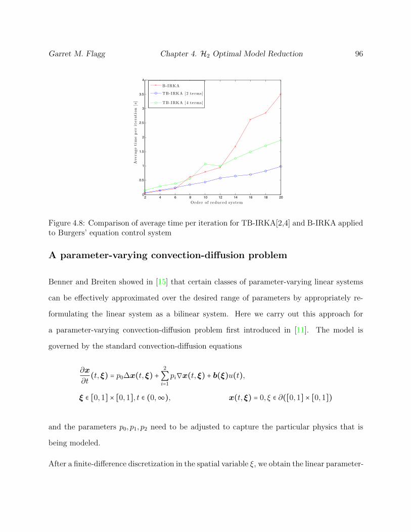
Garret M. Flagg Chapter 4. H2 Optimal Model Reduction 96
2 4 6 8 10 12 14 16 18 200
0.5
1
1.5
2
2.5
3
3.5
4
Order of reduced system
Avera
ge
tim
ep
er
itera
tion
[s]
B-IRKA
TB-IRKA [2 te rms]
TB-IRKA [4 te rms]
Figure 4.8: Comparison of average time per iteration for TB-IRKA[2,4] and B-IRKA appliedto Burgers’ equation control system
A parameter-varying convection-diffusion problem
Benner and Breiten showed in [15] that certain classes of parameter-varying linear systems
can be effectively approximated over the desired range of parameters by appropriately re-
formulating the linear system as a bilinear system. Here we carry out this approach for
a parameter-varying convection-diffusion problem first introduced in [11]. The model is
governed by the standard convection-diffusion equations
∂x
∂t(t,ξ) = p0∆x(t,ξ) +
2
∑i=1
pi∇x(t,ξ) + b(ξ)u(t),
ξ ∈ [0,1] × [0,1], t ∈ (0,∞), x(t,ξ) = 0, ξ ∈ ∂([0,1] × [0,1])
and the parameters p0, p1, p2 need to be adjusted to capture the particular physics that is
being modeled.
After a finite-difference discretization in the spatial variable ξ, we obtain the linear parameter-

Garret M. Flagg Chapter 4. H2 Optimal Model Reduction 97
0 5 10 15 20 25 300
5
10
15
20
25
30
Order of reduced system
Avera
ge
tim
eper
itera
tion
[s]
TB-IRKA [2 te rms]
TB-IRKA [4 te rms]
B-IRKA
Figure 4.9: Comparison of average time per iteration in TB-IRKA and B-IRKA for severalorders
varying dynamical system
x(t) = p0A0x(t) +2
∑i=1
Aix(t)pi + bu(t) (4.48)
y = cx(t),
where c = on is chosen as the observation matrix. This system can be viewed as a bilinear
system where the parameters p1 and p2 are particular system inputs. We can rewrite system
(4.48) as a bilinear system with three inputs and one output:
x =Ax +3
∑k=1
Nkxuk(t) +Bu(t)
y(t) = cx(t)
with A=p0A0, N1 = A1, N2 = A2, N3 = 0, B = [0,b] ∈ Rn×3, for inputs of interest

Garret M. Flagg Chapter 4. H2 Optimal Model Reduction 98
0 5 10 15 20 25 3010−4
10−3
10−2
10−1
100
Order of reduced system
Rel
ati
ve
H2
Err
or
TB-IRKA [2 te rms]
TB-IRKA [4 te rms]
B-IRKA
Figure 4.10: Comparison of TB-IRKA and B-IRKA approximations of heat transfer controlsystem
u(t) = [p1, p2, u(t)]T .
The parameter range of interest is p0 ∈ [0.1,1], p1, p2 ∈ [0,1] [11]. Taking p0 = 1 we computed
TB-IRKA approximations keeping 2,3, and 6 terms in the Volterra series, and compared
them with the B-IRKA approximation to the full bilinear system. Each of these approxima-
tions were of dimension r = 12. To place the reduced bilinear system matrices in the linear
parameter-varying formulation we took A = p0A0 ∈ Rr×r, N1 = A1 ∈ Rr×r and N2 = A2 as the
reduced-dimension matrices that approximate the linear parameter-varying system (4.48).
In order to evaluate the accuracy of the approximations, we varied the parameters p1 and p2
over the whole parameter range of interest, and for each selection of parameters we computed
the relative H2 norm of the error between the full and reduced dimension systems for that
choice of parameters. The surfaces plotted in Figure 4.11 show how the relative H2 error
of the linear systems varies over the parameter values. As Figure 4.11 shows, TB-IRKA[2
terms] actually gives the best approximation error over the parameter space, and the ap-
proximation error increases as the number of terms kept in the Volterra series increases, with
B-IRKA giving, in this case, the largest errors over the parameter space. We believe this is

Garret M. Flagg Chapter 4. H2 Optimal Model Reduction 99
due to the fact B-IRKA is actually a better approximation over the whole L2 unit ball of
inputs, and so it gives up some accuracy for these particular inputs. Next we computed a
TB-IRKA[2 terms] approximation and a B-IRKA approximation both of dimension r = 12
to approximate the bilinear system resulting from taking p0 = 0.5. Figure 4.12 shows the
relative H2 error in the linear systems over the parameter range for p0 = 0.5. Again for this
example, TB-IRKA[2 terms] yields a smaller approximation error than B-IRKA, and both
yield nearly uniform error over the range of parameters.
0 0.1 0.2 0.3 0.4 0.5 0.6 0.7 0.8 0.9 1 00.5
18e−5
2.8e−4
4.8e−4
6.84e−48e−4
p 2
p 1
Rel
ativ
e H 2 E
rror
TB−IRKA[6]TB−IRKA[3]TB−iRKA[2]B−IRKA
Figure 4.11: Convection-diffusion problem: Comparison of the relative H2 error in theB-IRKA and TB-IRKA[2, 3 and 6 terms] approximations taking p0 = 1 and varying over theparameter range for p1 and p2
4.1 Alternatives to H2 Optimal Bilinear Model Reduc-
tion
It is not uncommon to end up dealing with a bilinear system which does not have a convergent
H2 norm. For example, the bilinear system approximation ζ, to the nonlinear RC circuit
model first introduced by Skoogh and Bai is a standard benchmark model for testing methods

Garret M. Flagg Chapter 4. H2 Optimal Model Reduction 100
00.2
0.40.6
0.81
00.10.20.30.40.50.60.70.80.9110−5
10−4
10−3
10−2
p 1
Relative H2 error when p 0 = 0.5, r = 12
p 2
Rel
ativ
eH
2E
rror TB−IRKA [2 terms]
B−IRKA
Figure 4.12: Convection-diffusion problem: Comparison of the relativeH2 error in the B-IRKA and TB-IRKA[2 terms] approximations taking p0 = 0.5 and varying over the parameterrange for p1 and p2
of model reduction, but ζ /∈ F [6]. Other benchmark models, such as bilinear approximations
to Burgers’ equation are also not H2 for modest Reynolds numbers. In these situations,
there are a few options available. One technique is to scale ζ by the mapping
γ ↦ ζγ ∶= (A, γN , γb, c),
where γ < 1 is chosen sufficiently small so that ∥ζγ∥H2< ∞. H2 optimal model reduction is
carried out on ζγ, and the original input-output map can be recovered by scaling the inputs
u(t) for the original system by u(t)/γ.
Any truncation ζN of the original system has a finite HN2 norm. Computing an HN2 optimal
approximation to ζN using TB-IRKA is therefore another alternative when ζ is not H2.
Garret M. Flagg Chapter 4. H2 Optimal Model Reduction 101
Frequently an H2 optimal approximation of the first few terms in the Volterra series is
sufficiently accurate to match the output of the ζ.
Yet another approach is to match some combination of subsystem moments in the hopes of
capturing the dominant portion of the Volterra series for the inputs of interest.
Numerical Examples
TB-IRKA and the subsystem interpolation approach is demonstrated on an RC circuit model
of dimension 40,200. Solving the bilinear Sylvester equations required for B-IRKA was
beyond our computational resources for this model. We demonstrate the scaled B-IRKA
and TB-IRKA approaches on a control problem governed by the viscous Burger’s equations
first introduced in §4. The subsystem interpolation approach of Bai and Skoogh [6] that
matches moments about zero for the first and second order transfer functions is used as the
choice of moments in the subsystem interpolation approach.
Nonlinear RC circuit model
A bilinear model for an RC circuit with nonlinear resistors and an independent current
source was originally derived in [6]. This circuit was originally proposed by Chen and White
[32]. Let v1, . . . , vN be the N node voltages in the circuit and u(t) be the input-signal to the
independent current source. This circuit can be modeled by a linear-analytic model of the
form⎧⎪⎪⎪⎪⎨⎪⎪⎪⎪⎩
v = f(v(t)) + bu(t)
y(t) = cv(t), (4.49)
Garret M. Flagg Chapter 4. H2 Optimal Model Reduction 102
where
f(v) =
⎡⎢⎢⎢⎢⎢⎢⎢⎢⎢⎢⎢⎢⎢⎢⎢⎢⎢⎢⎢⎢⎢⎣
−g(v1) − g(v1 − v2)
g(v1 − v2) − g(v2 − v3)
⋮
g(vk−1 − vk) − g(vk − vk+1)
⋮
g(vN−1 − vN)
⎤⎥⎥⎥⎥⎥⎥⎥⎥⎥⎥⎥⎥⎥⎥⎥⎥⎥⎥⎥⎥⎥⎦
∈ RN b = cT =
⎡⎢⎢⎢⎢⎢⎢⎢⎢⎢⎢⎢⎢⎢⎣
1
0
⋮
0
⎤⎥⎥⎥⎥⎥⎥⎥⎥⎥⎥⎥⎥⎥⎦
∈ RN (4.50)
and g(v) = e40v(t) + v − 1. Taking a second order approximation of g(v) by matching the 2
terms of its MacLaurin series yields a quadratic nonlinear system. One can then apply the
Carleman linearization to this quadratic nonlinear system to obtain a bilinear model of the
nonlinear circuit. If the original linear-analytic model (4.49) is order N , the bilinear model
approximation is order n = N +N2. For this example, we take N = 200, so n = 40,200. We
compare the TB-IRKA approach with the Bai and Skoogh subsystem interpolation approach
for two standard test inputs: u(t) = e−t and u(t) = (cos(πt/10)+1)/2. Following the example
given in their paper [6] we constructed an order 21 reduced-order model that matched the
following moments about zero:
cA−q1b, for q1 = 1 . . . ,20 (4.51)
cA−1NA−q1b, for q1 = 1, . . . ,20 (4.52)
(4.53)
This approximation is compared to an order 13 approximation constructed from TB-IRKA,
where TB-IRKA was implemented by keeping the first two terms in the Volterra series.
Figures 4.13, 4.15 compares the response of the reduced order models to the true response
for inputs u(t) = e−t and u(t) = (cos(πt/10)+1)/2 respectively. Figures 4.14 and 4.16 compare

Garret M. Flagg Chapter 4. H2 Optimal Model Reduction 103
the relative error in the response As the figures illustrate, the true system responses are very
well matched by the TB-IRKA approximation.
0 0.5 1 1.5 2 2.5 3 3.5 40
0.002
0.004
0.006
0.008
0.01
0.012
0.014
0.016
0.018
Time [ s]
y(t
)
True Re sponse
TB - IRKA [2 te rms, r=13]
S ubsy stem Inte rpolat ion [ r=21]
Figure 4.13: Nonlinear RC Circuit: A comparison of the TB-IRKA and subsystem inter-polation response to the true response for the input u(t) = e−t
Burgers’ Equation Control System
In this example, we use the bilinear control system derived from Burgers’ equation introduced
§4. Here we take ν = 0.01, corresponding to a Reynolds number of 100 and construct a bilinear
system ζ of order n = 930. ζ is not an H2 system, which can be checked by observing that
the series used to compute its control grammian diverges. For this example we compared
TB-IRKA[2] with the scaled version of B-IRKA. An order r = 9 approximation is used to
compute the response of both methods to the inputs u(t) = e−t and u(t) = sin(20t). The
relative error in the output of using the scaling values γ = 0.4,0.5 for B-IRKA are compared
with the TB-IRKA[2] approximation in Figures 4.17, 4.18. As the figures show, very good
approximation results using B-IRKA can be obtained for the right value of γ, in this case
γ = 0.4 yielded good approximations, but the quality of the approximations is fairly sensitive

Garret M. Flagg Chapter 4. H2 Optimal Model Reduction 104
0 0.5 1 1.5 2 2.5 3 3.5 410−7
10−6
10−5
10−4
10−3
10−2
10−1
100
Time [ s]
Rel
ati
ve
Abso
lute
Err
or
Su bsy stem Inte rpolation [ r=21]
TB - IRKA [2 te rm s, r=13]
Figure 4.14: Nonlinear RC Circuit: A comparison of the TB-IRKA and subsystem inter-polation error for the input u(t) = e−t
to the choice of γ. For both inputs the TB-IRKA[2] approximation yields a highly accurate
approximation, and indeed is more accurate than B-IRKA on the whole time interval of [0,4]
seconds for the input u(t) = e−t.

Garret M. Flagg Chapter 4. H2 Optimal Model Reduction 105
0 1 2 3 4 5 6 7 8 9 100
0.005
0.01
0.015
0.02
0.025
Time [ s]
y(t
)
True Re sponse
TB - IRKA [2 te rm s, r=13]
Su bsy stem Inte rpolation [ r=21]
Figure 4.15: Nonlinear RC Circuit: A comparison of the TB-IRKA and subsystem inter-polation response to the true response for the input u(t) = (cos(πt/10) + 1)/2
0 1 2 3 4 5 6 7 8 9 1010−9
10−8
10−7
10−6
10−5
10−4
10−3
10−2
10−1
100
Rel
ati
ve
Abso
lute
Err
or
T ime [ s]
Su bsystem [ r=21]
TB-IRKA [2 te rms, r=13]
Figure 4.16: Nonlinear RC Circuit: A comparison of the TB-IRKA and subsystem inter-polation error for the input u(t) = (cos(πt/10) + 1)/2
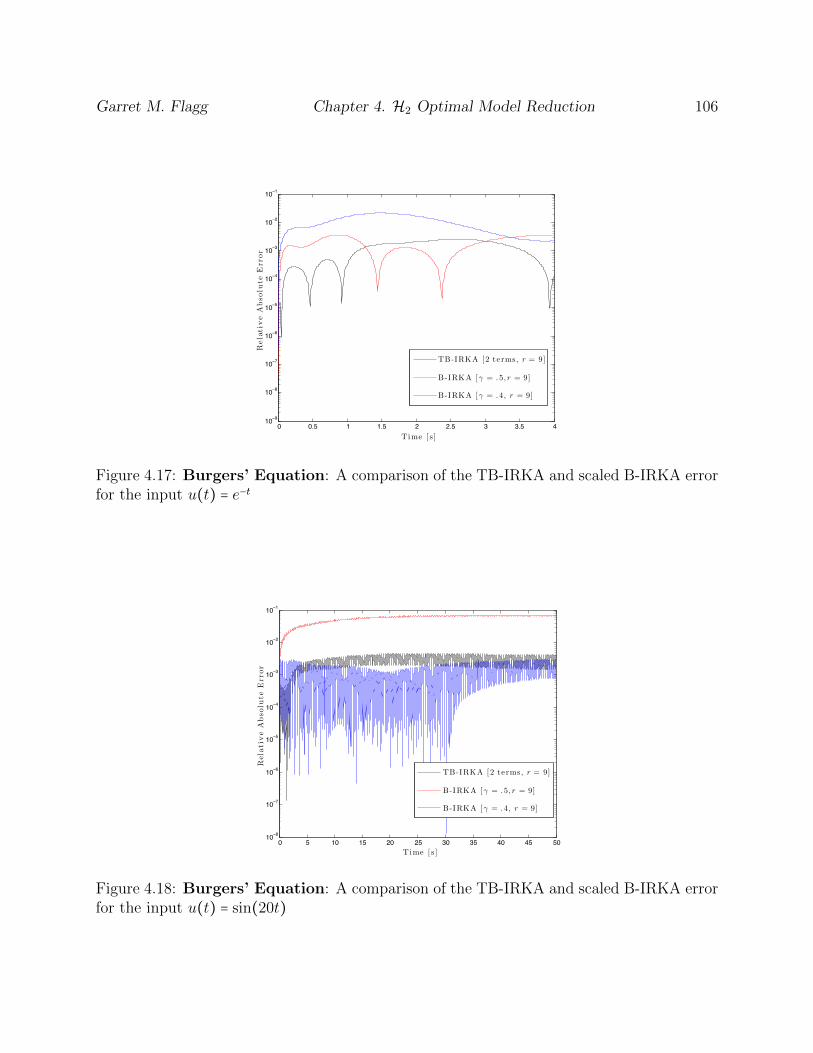
Garret M. Flagg Chapter 4. H2 Optimal Model Reduction 106
0 0.5 1 1.5 2 2.5 3 3.5 410−9
10−8
10−7
10−6
10−5
10−4
10−3
10−2
10−1
Time [ s]
Rela
tive
Abso
lute
Err
or
TB-IRKA [2 te rms, r = 9]
B-IRKA [γ = .5,r = 9]
B-IRKA [γ = .4, r = 9]
Figure 4.17: Burgers’ Equation: A comparison of the TB-IRKA and scaled B-IRKA errorfor the input u(t) = e−t
0 5 10 15 20 25 30 35 40 45 5010−8
10−7
10−6
10−5
10−4
10−3
10−2
10−1
Time [ s]
Rel
ati
ve
Abso
lute
Err
or
TB-IRKA [2 te rms, r = 9]
B-IRKA [γ = .5,r = 9]
B-IRKA [γ = .4, r = 9]
Figure 4.18: Burgers’ Equation: A comparison of the TB-IRKA and scaled B-IRKA errorfor the input u(t) = sin(20t)
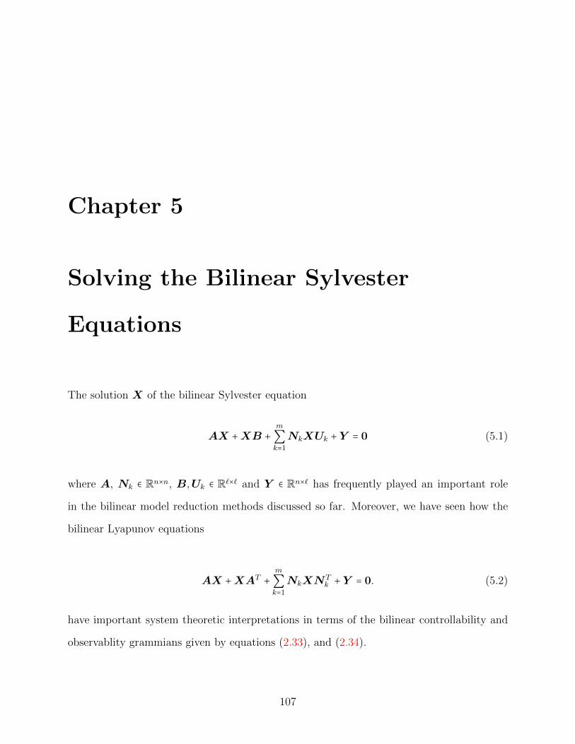
Chapter 5
Solving the Bilinear Sylvester
Equations
The solution X of the bilinear Sylvester equation
AX +XB +m
∑k=1
NkXUk +Y = 0 (5.1)
where A, Nk ∈ Rn×n, B,Uk ∈ R`×` and Y ∈ Rn×` has frequently played an important role
in the bilinear model reduction methods discussed so far. Moreover, we have seen how the
bilinear Lyapunov equations
AX +XAT +m
∑k=1
NkXNTk +Y = 0. (5.2)
have important system theoretic interpretations in terms of the bilinear controllability and
observablity grammians given by equations (2.33), and (2.34).
107

Garret M. Flagg Chapter 5. Solving the Bilinear Sylvester Equations 108
When all Nk or Uk = 0, (5.1) reduces to the standard Sylvester equation
AX +XB +Y = 0. (5.3)
In the next two sections we will discuss both direct and iterative methods for solving large-
scale bilinear Sylvester equations, with special attention to the bilinear Lyapunov equations.
In the third section we will present a new analysis of rational Krylov projection methods
for solving Sylvester equations and their connection to the ADI method. We will then
consider the generalization of these results to bilinear Sylvester equations. These results
provide insight into the advantages and limitations of using Krylov projection methods in
the bilinear case.
5.1 Direct Methods
Perhaps the most brute force approach to solving (5.1) is to transform it into a linear system
by applying the vec operator to it, which yields the nm-dimensional linear system
− (I ⊗A +BT ⊗ I +m
∑k=1
UTk ⊗Nk)vec(X) = vec(Y ). (5.4)
and X can be found by inverting the nm-dimensional linear operator T = −(I⊗A+BT ⊗I +m
∑k=1UTk ⊗Nk). The computational complexity of using this approach directly is O((nm)3),
which makes it untenable for nearly all large-scale applications. This effectively exhausts
all known direct methods for solving the full bilinear Sylvester equations. Unless otherwise
specified, we will therefore consider the bilinear Lyapunov equations exclusively in what
follows.
Garret M. Flagg Chapter 5. Solving the Bilinear Sylvester Equations 109
A more efficient direct method of solution based on the Sherman-Morrison-Woodbury for-
mula exploits the fact that the Nk are typically low rank. This approach was developed by
E.G. Collins, Jr. et. al. in [33], [79]. The lefthand side of equation (5.2) can be viewed
as the sum of the linear operators LA(X) = AX +XAT and Π(X) =m
∑k=1NkXNT
k . If
rank(Nk) = rk ≪ n, then the rank of Π is bounded above by r0 =m
∑k=1
r2k. Assume that
for each Nk, a rank revealing factorization is available, and that rank(Π) = r ≪ n2. Then
vec(Π) may be factored as P1P2, where P2 ∈ Rr,n2and P1 ∈ Rn2,r. One may then apply the
following lemma, which is a variant of the Sherman-Morrison-Woodbury formula, to obtain
the solution of equation (5.2).
Lemma 5.1. Let L,P ∈ Rn×n, and consider the linear equation
(L +P )x = y. (5.5)
Suppose P = P1P2 where P2 ∈ Rr,n and P1 ∈ Rn,r, and that L is invertible. Then equation
(5.5) is uniquely solvable if and only if I +P2L−1P1 is nonsingular. If w solves
(Ir +P2L−1P1)w = P2L
−1y
then x = L−1(y −P1w) solves equation (5.5).
The direct inversion of LA can be done in O(n3) operations using the Bartels-Stewart al-
gorithm [10]. If a rank revealing factorization of Π is indeed available, then (5.2) may be
solved in max{O(n3r),O(r3)} operations [37]. If in addition the Nk’s, k = 1, . . . ,m, must be
factorized, then (5.2) may be solved in O(mn3+r20n
2+rn3) operations [37]. For an algorithm
that achieves this estimate and details the factorization of the Nk’s and Π, see [37].

Garret M. Flagg Chapter 5. Solving the Bilinear Sylvester Equations 110
5.2 Iterative Methods
There are several iterative methods for solving the bilinear Lyapunov equations, all of which
are based on the following results on convergent regular splittings due to H. Schneider [84].
The following is a brief summary of the iterative approaches introduced by Damm in [37].
Throughout the discussion, σ(T ) ⊂ C denotes the spectrum of a linear operator T , and
ρ(T ) = max{∣λ∣ ∶ λ ∈ σ(T )} denotes the spectral radius.
Theorem 5.1. Let A ∈ Rn×n and consider linear operators LA,Π ∶ Rn×n → Rn×n, where
LA =AX +XAT , and Π is nonnegative in the sense that Π(X) ≥ 0, whenever X ≥ 0. The
following are equivalent:
a.) ∀Y > 0,∃X > 0 s.t. LA(X) +Π(X) = −Y ,
b.) ∃Y ,X > 0 s.t. LA(X) +Π(X) = −Y ,
c.) ∃Y , with (A,Y ) controllable s.t. ∃X > 0 and LA(X) +Π(X) = −Y ,
d.) σ(LA +Π) ⊂ C−,
e.) σ(LA) ⊂ C− and ρ(L−1A Π) < 1.
If ρ(L−1A Π) < 1, then (LA +Π)−1 is given by the Neumann series
(LA +Π)−1 =∞
∑k=0
(L−1A Π)k(L−1
A ), (5.6)
which leads to the most obvious iterative scheme
Xk+1 = L−1A Π(Xk) +L
−1A (Y ) (5.7)
Garret M. Flagg Chapter 5. Solving the Bilinear Sylvester Equations 111
that we have already been applying liberally throughout the proofs in the multipoint Volterra
series interpolation discussion. Although this iteration is guaranteed to converge to the
solution, the convergence may be very slow. A more sophisticated iterative method uses
Krylov-subspace methods such as GMRES (generalized minimum residual) to minimize the
residual Rk =Xk+1 −Xk, see [37]. For larger problems, inverting LA may still be too costly.
In this case, one can use the ADI method as a kind of preconditioner. The ADI method
was first introduced by Peaceman and Rachford [75] as a method for solving parabolic and
elliptic PDEs, and was later adapted to solving the Sylvester equation by Wachspress in
[97]. It is a fixed point iteration scheme for approximating the solution X to the ordinary
Sylvester equation
AX +XB +Y = 0. (5.8)
that has been developed extensively, see [76, 18, 17, 68, 55, 90, 89, 57, 83, 97, 93, 98]. Given
two sequences of shifts {α1, α2, . . . , αr, . . .},{β1, β2, . . . , βr, . . .} ⊂ C and an initial guess X0,
the ADI iteration proceeds as follows :
Xi =(A − αiI)(A + βiI)−1Xi−1(B − βiI)(B + αiI)
−1 (5.9)
− (αi + βi)(A + βiI)−1Y (B + αiI)
−1. (5.10)
This iteration can be generalized to the bilinear Lyapunov equation by observing that for a
given shift α ∈ R ∖ {0},
LA(X) =1
2α((A + αI)−1X(A + αI)T − (A − αI)X(A − αI)T ) (5.11)

Garret M. Flagg Chapter 5. Solving the Bilinear Sylvester Equations 112
Thus, (5.2) can be written in the fixed-point form
X = (A+αI)−1(A−αI)X(A+αI)−T (A−αI)T −2α(A+αI)−1(m
∑j=1
NjXNTj +Y )(A+αI)−T
(5.12)
The ADI iteration can now be interpreted as a preconditioning technique in the following
way. For given ADI-parameters α` < 0 ` = 1, . . . , L and Xk, define the iterations
Xk+ lL= (A + α`I)
−1(A + α`I)Xk+ l−1L(A + α`I)
−T (A − α`I)T
− 2α`(A + α`I)−1(
m
∑j=1
NjXkNTj +Y )(A + α`I)
−T (5.13)
Setting
G0 =L
∏`=1
(A + α`I)−1(A − α`I),
Gp = (L
∏`=p+1
(A + α`I)−1(A − α`I))(A + αpI)
−1, for p = 1, . . . , L
a single iteration on Xk can then be written as
Xk+1 = G0XkGT0 +
L
∑p=1
2αp(m
∑j=1
(GpNj)Xk(GpNj)T +GpY G
Tp ) (5.14)
[37]. The kth step in this iteration is equivalent to applying L steps of the ADI iteration at
the kth term in the series (5.6), and therefore at best it will converge at the same rate as the
iteration in (5.7). The obvious advantage to this approach is that provides an inexpensive
way to approximate L−1A and can therefore be applied as a preconditioning technique in an
iterative method like GMRES [37].
Garret M. Flagg Chapter 5. Solving the Bilinear Sylvester Equations 113
5.3 Krylov projection-based approximation of ordinary
Sylvester equations
In this section, we will make a brief excursion into the analysis of rational Krylov projection
methods (RKPM) for the ordinary Sylvester equations. In the next section, we will generalize
our results to the bilinear case. Throughout this section Y is the rank one matrix Y =
bc for Sylvester equations and in the context of Lyapunov equations we will take Y =
bb∗. I will present new results that connect the RKPM with the ADI iteration for linear
systems. The RKPM is the presiding alternative to the ADI iteration for solving large-
scale Sylvester equations [58, 61, 38, 60, 85, 91, 42, 9]. In the RKPM, the Sylvester equation
AX+XB+Y = 0 is projected onto the rational Krylov subspaces Kratr (A,b,σ) = span{(σ1I−
A)−1b, . . . , (σrI −A)−1b} and Kratr (B∗,c, µ) where σ= {σ1, . . . σr}, and µ = {µ1, . . . , µr} are
the sets of shifts used to construct the respective rational Krylov spaces and ν denotes the
conjugate of ν. See [12] for further details regarding Kratr (A,b,σ), and constructing an
orthonormal basis via the rational Arnoldi iteration. Let Qr and Ur denote the orthonormal
basis for Kratr (A,b,σ) and Krat
r (B∗,c, µ). Then, the RKPM approximation is constructed
by first solving
Q∗rAQrXr + XrU
∗rB
∗Ur +Q∗rbc
∗Ur = 0 (5.15)
and then approximating X by QrXrU∗r . The solution of the projected Sylvester equation
(5.15) is inexpensive. Like the ADI method, the RKPM method also relies heavily on a
good choice of shifts to produce accurate results. The main result is that the ADI iteration
and rational Krylov projection-based methods are equivalent for the special case of shifts
satisfying condition (1) in Theorem 4.2. I will call these shifts pseudo-H2 optimal shifts.
Recently, Breiten and Benner showed that these shifts are also locally optimal with respect
to a special energy norm related to the Lyapunov equations for Hermitian linear dynamical

Garret M. Flagg Chapter 5. Solving the Bilinear Sylvester Equations 114
systems [21]. The main equivalence theorem requires the following lemma, which connects
the ADI approximation for the Sylvester equation with rational Krylov subspaces. This
extends an earlier result by Li and White [67] which establishes a similar connection for the
the case of the Lyapunov equation.
Lemma 5.2. Let Q = bc∗, where b ∈ Rn and c ∈ Rm. Let {σ1, . . . , σr} and {µ1, . . . , µr}
be two collections of shifts that satisfy R(µi),R(σi) > 0 for i = 1, . . . , r. Suppose Xr is the
approximate solution to the Sylvester equation (5.3) obtained by applying the pair of shifts
αi = −σi and βi = −µi in the ADI iteration (5.9) for i = 1, . . . , r with X0 = 0. Then there
exist Lr ∈ Cn×r and Rr ∈ Cm×r such that Xr = LrR∗r and colspan(Lr) ⊂ Krat
r (A,b,µ) and
colspan(Rr) ⊂ Kratr (B∗,c, σ)
Proof. The proof is given by induction on i, the iteration step. First note that for i = 1,
X1 = (µ1 + σ1)(A − µ1I)−1bc∗(B − σ1I)−1, so let L1 = [(µ1 + σ1)(A − µ1I)−1b] and R1 =
[(B∗ − σ1I)−1c]. Then L1 and R1 clearly satisfy the hypothesis and X1 = L1R∗1 . Now
suppose that the statement holds for Xi. Then, for j = 1, . . . , i, the jth column of Li is
T(j)i (A)b, where T
(j)i (λ) is a proper rational function that lies in the span of { 1
λ−µ1, . . . , 1
λ−µi}.
Similarly, the jth column ofRi is S(j)i (B∗)c, where S
(j)i (λ) lies in the span of { 1
λ−σ1, . . . , 1
λ−σi}.
Therefore Xi+1 can be written as
Xi+1 =(A + σi+1I)(A − µi+1I)−1LR∗(B + µi+1I)(B − σi+1B)−1
+ (µi+1 + σi+1)(A − µi+1I)−1bc∗(B − σi+1I)
−1
=i
∑j=1
(A + σi+1I)(A − µi+1I)−1T
(j)i (A)bc∗S
(j)i (B)(B + µi+1I)(B − σi+1I)
−1
+ (µi+1 + σi+1)(A − µi+1I)−1bc∗(B − σi+1I)
−1
For j = 1, . . . i, let the jth column of Li+1 be (A + σi+1I)(A − µi+1I)−1T(j)i (A)b and let the

Garret M. Flagg Chapter 5. Solving the Bilinear Sylvester Equations 115
(i + 1)th column be T(i+1)i+1 (A)b = (µi+1 + σi+1)(A − µi+1I)−1b. Then clearly colspan(Li+1) ⊂
Krati+1(A,b,µ). Similarly, let (B∗ − σi+1I)−1(B∗ + µi+1I)S
(j)i (B∗)c be the jth column of
Ri+1 for j = 1, . . . , i, and S(i+1)i+1 (B∗)c = (B∗ − σi+1I)−1c be the (i + 1)th column. Then
colspan(Ri+1) ⊂ Krati+1(B
∗,c, σ). Finally, we note that by construction, Xi+1 = Li+1R∗i+1.
Next, we present our equivalency result, showing that the approximate solution of the
Sylvester equation (5.3) by ADI and RKPM are indeed equivalent when the shifts are cho-
sen as pseudo-H2 optimal points. This result applied to the special case of the Lyapunov
equations was first presented at the 2010 SIAM Annual Meeting [44] then later published
independently in [38]. Our new result here, on the other hand, is more general than both [44]
and [38] since it tackles the case of Sylvester equation and includes the Lyapunov equation
as a special case. Moreover, while the proof given in [38] for the special case of Lyapunov
equation makes use of a novel connection between the ADI iteration and the so-called Skele-
ton approximation framework first developed in the work of Tyrtyshnikov [94], the proof
we provide here for the more general Sylvester equation case is given directly in terms of
rational Krylov interpolation conditions, and in that sense is simpler.
Theorem 5.2. Given the Sylvester equation (5.3) with Y = bc∗, where b ∈ Rn and c ∈ Rm,
let Qr ∈ Rn×r be an orthonormal basis for the rational Krylov subspace Kratr (A,b,σ) and let
Ur ∈ Rm×r be an orthonormal basis for the rational Krylov subspace Kratr (B∗,c, σ) for a set
of shifts σ = {σ1, . . . , σr} where R(σi) > 0 for i = 1, . . . , r. Let Xr ∈ Rr×r solve the projected
Sylvester equation
Q∗rAQrXr + XrU
∗rBUr +Q
∗rbc
∗Ur = 0, (5.16)
and let Xr ∈ Rn×m be computed by applying the shifts αi = −σi and βi = −σi to exactly r
steps of the ADI iteration (5.9) for i = 1, . . . , r. Then Xr = QrXrU∗r if and only if either
λ(Q∗rAQr) = −{σ1, . . . , σr} or λ(U∗
rBUr) = −{σ1, . . . , σr}.

Garret M. Flagg Chapter 5. Solving the Bilinear Sylvester Equations 116
Proof. (⇐) First suppose that λ(Q∗rAQr) = −{σ1, . . . , σr}. The proof remains the same
if we instead suppose that λ(U∗rBUr) = −{σ1, . . . , σr}. Let A = Q∗
rAQr, and b = Q∗rb,
Br = U∗rBUr, and c = U∗
r c. Note that after we apply r steps of the ADI iteration with the
set of shifts αi = βi = −σi to the projected Sylvester equation (5.16), we obtain the exact
solution Xr, since λ(A) = −{σ1, . . . , σr}. By Lemma 5.2, at the rth step of the ADI iteration
Xr = LrR∗r where Lr = [T (1)(A)b, . . . , T (r)(A)b] where T (i)(A)b are rational functions that
lie in Kratr (A, b,σ). Similarly Rr = [S(1)(B∗
r )c∗, . . . , S(r)(B∗
r )c∗] where the S(i)(B∗
r )c are
rational functions that lie in Kratr (B∗
r , c∗, σ). Furthermore, for the same shifts, αi = βi = −σi
for i = 1, . . . , r, applied to r steps of the ADI iteration on the full Sylvester equation (5.3), we
have Xr = LrR∗r and Lr = [T (1)(A)b, . . . , T (r)(A)b] and Rr = [S(1)(B∗)c, . . . , S(r)(B∗)c].
Thus it is sufficient to show that QrLr = Lr and that UrRr =Rr. Without loss of generality
consider just the former equation. This, in turn, amounts to showing that QrT (i)(A)b =
T (i)(A)b. If Ti(A)b are a set of orthogonal rational functions that span Kratr (A,b,σ), then
it is sufficient to show that
QrTi(A)b = Ti(A)b. (5.17)
Equality (5.17) follows readily from the interpolation properties of the Galerkin projection,
which we show below. First, note that due to the interpolation properties of the Galerkin
projection, Qr(σiIr − A)−1b = (σiI −A)−1b. Let V = [(σ1I −A)−1b . . . (σrI −A)−1b]. Then,
for some x ∈ Rr,
V x = Ti(A)b =Qr[(σ1Ir − A)−1b . . . (σrIr − A)−1b]x =QrTi(A)b, (5.18)
which proves (5.17). (⇒) Let Xr be the solution of
Q∗rAQrXr + XrU
∗rBUr +Q
∗rbc
∗Ur = 0 (5.19)

Garret M. Flagg Chapter 5. Solving the Bilinear Sylvester Equations 117
where Qr is an orthonormal basis for Kratr (A,b,σ) and Ur is an orthonormal basis for
Kratr (B∗,c, σ). Suppose that QrXrU∗
r =Xr. Let Xr be the approximate solution of (5.19)
resulting from applying the shifts αi = βi = −σi for i = 1, . . . , r to exactly r steps of the ADI
iteration (5.9). By the interpolation result given in the proof above, QrXrU∗r = Xr. It
follows from the assumptions that, QrXrU∗r = QrXrU∗
r , so Xr = Xr. But this means that
Xr solves (5.19), and so either λ(Q∗rAQr) = −{σ1, . . . , σr} or λ(U∗
rBUr) = −{σ1, . . . , σr}.
The parameters for which the ADI iteration and the rational Krylov projections coincide
also satisfy orthogonality conditions on the residual for the special case of the Lyapunov
equation
AX +XA∗ + bb∗ = 0 (5.20)
For a given approximation Xr to the solution X, define the residual R as
R =AXr +XrA∗ + bb∗. (5.21)
The following result was first given in [38]. Here we present a new and more concise proof
of the orthogonality result in terms of the special interpolation properties of the pseudo
H2-optimal shifts.
Theorem 5.3. Given AX +XA∗ + bb∗ = 0, let Xr ∈ Rr×r solve the projected Lyapunov
equation
Q∗rAQrXr + XrQ
∗rAQr +Q
∗rbb
∗Qr = 0,
where Qr is an orthonormal basis for the Kratr (A,b,σ) with σ = {σ1, . . . , σr} Let Xr =
QrXrQ∗r .Then Q∗
rR = 0 if and only if λ(Q∗rAQr) = −{σ1, . . . , σr} where R is the residual
defined in (5.21).
Proof. (⇒) Suppose that Q∗rR = 0. Multiplying (5.21) with Q∗
r from the left and then

Garret M. Flagg Chapter 5. Solving the Bilinear Sylvester Equations 118
transposing the resulting equation leads to
AQrXr +QrXrQ∗rA
∗Qr + bb∗Qr = 0. (5.22)
Let A =Q∗rAQr = TΛT −1 be the eigenvalue decomposition of A where Λ = diag(λ1, . . . , λr).
Plug these expressions into (5.22), and right multiply by T −∗ to obtain
QrXrT−∗Λ∗ +AQrXrT
−∗ + bb∗QrT−∗ = 0 (5.23)
Let ζi be the ith entry of b∗QrT −∗. Then it is straightforward to show that the ith column
of QrXrT −∗ must be (−λiI −A)−1bζi. Thus, it follows that Kratr (A,b,σ) = Krat
r (A,b,−λ),
where λ = {λ1, . . . , λr}. Since both sets σ and λ are closed under conjugation, after an
appropriate reordering, we obtain σi = −λi.
(⇐) Observe that
AXr + XrA∗ +Q∗
rbb∗Qr = 0⇒ (5.24)
AXrT−∗ + XrT
−∗Λ∗ +Q∗rbb
∗QrT−∗ = 0. (5.25)
Thus, the ith column of XrT −∗ is (−λiIr−A)−1Q∗rbζi. But since Qr is an orthonormal basis
for Kratr (A, b,σ), and λi = −σi, this means
Qr(−λiIr − A)−1Q∗rbζi = (−λiI −A)−1bζi = (QrXrT
−∗)ei, (5.26)
where ei is the ith unit vector. Thus,
QrXrT−∗Λ∗ +AQrXrT
−∗ + bb∗QrT−∗ = 0, (5.27)

Garret M. Flagg Chapter 5. Solving the Bilinear Sylvester Equations 119
which implies
QrXrQ∗rA
∗Qr +AQrXr + bb∗Qr = 0. (5.28)
Transpose this last expression and use the fact that Q∗rQr = Ir to obtain
Q∗rQrXrQ
∗rA
∗ +Q∗rAQrXrQ
∗r +Q
∗rbb
∗ =Q∗rR = 0, (5.29)
which is the desired result.
Numerical examples for LTI systems
Here we present two numerical examples illustrating the accuracy of the RKPM method using
pseudo-H2 optimal shifts applied to LTI systems. Three different approximation methods
are compared for each model.
• Method 1: The RKPM is applied to the a sequence of shifts that alternates between 0
and ∞. The resulting subspace is generally referred to as the extended Krylov subspace.
Its application to RKPM was first introduced by Simoncini in [85].
• Method 2: The RKPM is applied using r pseudo-H2 optimal shifts; or equivalently r
steps the ADI iteration is applied using r pseudo-H2 optimal shifts.
• Method 3: r-steps of the ADI iteration are applied, where the ADI shifts are chosen
via Penzl’s heuristic method [76].

Garret M. Flagg Chapter 5. Solving the Bilinear Sylvester Equations 120
The Eady model
The first example is an Eady model used for atmospheric storm tracking. The full order
model is order 598. For more information about this model, see [30]. All three methods are
used to approximate the controllability grammian P of the system. The approximations are
compared in both the induced-2 norm, where the SVD the approximation is optimal. It is
clear from Figure 5.1 that the Method 2 outperforms Method 1 and Method 3 for all ranks
of approximation, and that it yields a nearly optimal approximation in the 2-norm.
5 10 15 20 25 30 35 40 45 5010−10
10−8
10−6
10−4
10−2
Rank
||X−
Xk|| 2
/||X
|| 2
πk + 1/π 1
M etho d 1
M e tho d 2
M e tho d 3
Figure 5.1: Relative error in the 2-norm as r varies for the EADY Model
Rail Model
This model arises from a semidiscretized heat transfer problem for the optimal cooling of
steel profiles during a cooling process for a rolling mill. See [19], for further information on
this model. The the order of the full model is n = 1357. In this example, Figure 5.2 shows
that methods 2 and 3 perform comparably, but notably this is in large part due to the fact
that the collection of shifts chosen in Penzl’s heuristic in method 3 distribute themselves
closely to the distribution of pseudo-H2 optimal shifts. Both methods 2 and 3 yield very

Garret M. Flagg Chapter 5. Solving the Bilinear Sylvester Equations 121
accurate approximations in the matrix 2-norm for each rank.
0 2 4 6 8 10 12 14 16 18 2010−8
10−7
10−6
10−5
10−4
10−3
10−2
10−1
100
101
Rank
||X−
Xk|| 2
/||X
|| 2
π k + 1/π 1
M etho d 1
M etho d 2
M etho d 3
Figure 5.2: Relative error in the 2-norm as r varies for the Rail Model
5.4 Krylov projection-based methods for the approxi-
mation of the bilinear Lyapunov equations
We now generalize the orthogonality results of the previous section to the bilinear Lyapunov
equations. The results are presented for SISO bilinear systems to simplify the presentation,
but can readily be extended to MIMO systems. Let X be any approximation to the solution
X of the bilinear Lyapunov equations
AX +ATX +NXNT + bbT = 0.
Define the residual R as
R =AX + XAT +NXNT +Q = 0.
Theorem 5.4. Consider a SISO bilinear system ζ=(A, N , b, c). Let Qr be an orthonormal

Garret M. Flagg Chapter 5. Solving the Bilinear Sylvester Equations 122
basis for V which solves the multipoint Volterra series interpolation problem (3.31) for shifts
σi = −λ(QTrAQr) and weight matrix U = T −1QT
rNQrT , where TΛT −1 = A is the eigenvalue
decomposition of A =QTrAQr. Let Xr, solve the projected bilinear Lyapunov equations
AXr + XrA + NXrNT + bbT = 0.
Then the residual Rr of the approximation Xr = QrXrQTr is orthogonal to Qr. Moreover,
if Qr∈ Rn×r is any orthonormal matrix of rank r, define A, N , b, c in the usual way, and let
TΛT −1 = A be the usual eigenvalue decomposition. If Xr = QrXrQTr where Xr solves the
projected bilinear Lyapunov equations and QTrRr = 0, then ζr interpolates ζ in the points
−λj(A) with weights U = T −1QTrNQrT .
Proof. For the first part, we show that the residual is orthogonal to the projection subspace.
By hypothesis,
AXr + XrA + NXrNT + bbT = 0 ⇒
AXrT−T + XrT
−TΛ + NXrT−TUT + bbTT −T = 0
By the construction in the proof of Theorem 3.3, the jth column of XrT −T is given as the
weighted Volterra series (3.33) with the weights and shifts given in the hypotheses, and since
Qr is an orthonormal basis for V , QrXrT −T solves
V (−Λ) −AV −NV UT − bbTT −T = 0

Garret M. Flagg Chapter 5. Solving the Bilinear Sylvester Equations 123
Therefore
QrXrT−TΛ +AQrXrT
−T +NQrXrT−TUT + bbTT −T = 0 ⇒
QrXrQTrA
TQr +AQrXr +NQrXrQTrN
TQr + bbQTr = 0
Transposing this last equality and using the fact that QTrQr = Ir gives
QTr (AXr +XrA
T +NXrNT + bbT ) = 0
QTr (Rr) = 0
Now suppose that Qr ∈ Rn×r is a rank r orthonormal matrix that satisfies the hypothesis of
the second part. Then
QTr (AXr +XrA
T +NXrNT + bbT ) = 0
AXrQTr + XrQ
TrA
T + NXrQTrN
T + bbT = 0 ⇒
QrXrT−T (−Λ) −AQrXrT
−T −NQrXrT−TUT − bbTr = 0
So again, V =QrXrT −T solves the interpolation problem in the points −λ(A) and weights
U = TNT −1. ζr resulting from the projection onto V and along (V T V )−1V T differs from
the system ζr by the similarity transformation T TX−1r , and therefore ζr interpolates ζ in
the points −λ(A) and weights U .
Note that in the bilinear case the interpolation conditions are necessary and sufficient, but
the projection subspaces are not necessarily determined by the weights in U , and the points
σi. This is due to the fact that there is no underlying function space for the Volterra

Garret M. Flagg Chapter 5. Solving the Bilinear Sylvester Equations 124
series interpolation problem with functions that are uniquely determined by the choice of
interpolation points and weights, as is the case for rational Krylov subspaces.
These orthogonality conditions can be used to show that the one-sided interpolation condi-
tions are optimal for Hermitian bilinear systems in a special matrix inner product. Suppose
A, N are Hermitian, the pair (A, b) is controllable, and a solution to the bilinear Lyapunov
equation with Y = bbT exists. By Theorem 5.1, σ(LA +Π) ⊂ C−, and since LA +Π is Her-
mitian, T = −(I ⊗A +A⊗ I +N ⊗N) is positive definite. Following Vandereycken in [95],
we can define the inner product
⟨x,y⟩T = yTT x
and define the corresponding norm
∥x∥T =√
⟨x,x⟩T
which we will call the induced energy norm of the bilinear system. The orthogonality con-
ditions given in Theorem 5.4 yield the following optimality result in the the induced energy
norm.
Theorem 5.5. Let ζ have state-space realization (A,N ,b,cT ), and suppose A,N , are Her-
mitian. Let Xr satisfy the hypotheses of Theorem 5.4. Then Xr is optimal over the subspace
Z = {Z ∶ Z =QrZQTr , Z ∈ Rr×r} in the induced energy norm.
Proof. Note that Z is closed and convex. By the standard Hilbert space projection theorem
[66], optimality is equivalent to ⟨vec(X −Xr), vec(Z)⟩T = 0 for any Z ∈ Z. By the definition
of the T inner product
Garret M. Flagg Chapter 5. Solving the Bilinear Sylvester Equations 125
⟨vec(X −Xr), vec(Z)⟩T = 0
⇐⇒ trace(ZT (LA +Π)(X −Xr)) = 0
⇐⇒ trace(QrZ(QTrRr)) = 0,
and this last equality clearly obtains for the approximation Xr.
Bilinear heat transfer system
The controllability grammian P of the bilinear heat transfer system first introduced in
Chapter 4. of order n = 10,000 is approximated. For this system the operator L is Hermitian
positive definite, so the L-norm of the grammian exists. The pseudo-H2 approximations are
compared with the SVD approximation in both the L-norm and the Frobenius norm in
Figures 5.4 and respectively. As expected from our results in Theorem 5.4, the pseudo-H2
projection subspace outperforms the SVD in the L-norm for each rank of approximation,
but the rank r SVD approximation performs better in the Frobenius norm. In either case,
there is little difference in the quality of the approximations.
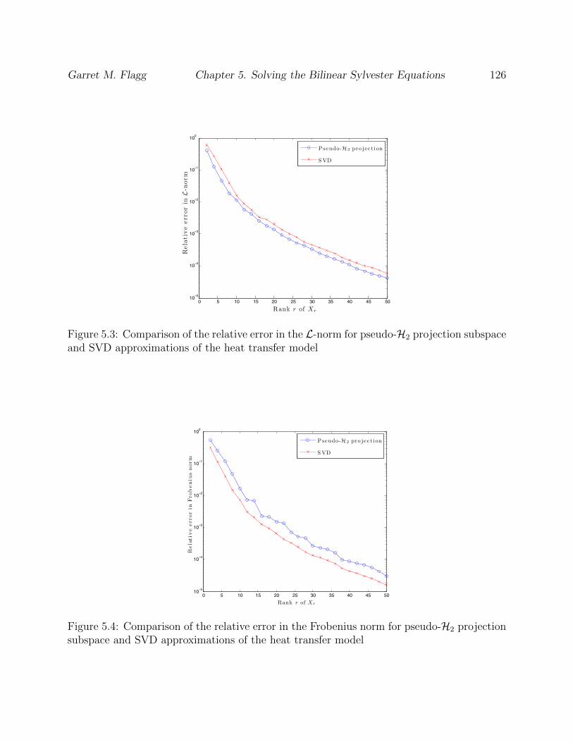
Garret M. Flagg Chapter 5. Solving the Bilinear Sylvester Equations 126
0 5 10 15 20 25 30 35 40 45 5010−5
10−4
10−3
10−2
10−1
100
Rela
tive
err
or
inL-
norm
Rank r of Xr
Pseudo-H 2 pro je c t i on
S VD
Figure 5.3: Comparison of the relative error in the L-norm for pseudo-H2 projection subspaceand SVD approximations of the heat transfer model
0 5 10 15 20 25 30 35 40 45 5010−5
10−4
10−3
10−2
10−1
100
Rela
tive
err
or
inFro
beniu
snorm
Rank r of Xr
Pseudo-H 2 pro je c t i on
S VD
Figure 5.4: Comparison of the relative error in the Frobenius norm for pseudo-H2 projectionsubspace and SVD approximations of the heat transfer model

Chapter 6
Data-Driven Model Reduction of
SISO Bilinear Systems
In this section we present a solution to the following bilinear realization problem: Suppose
we have data corresponding to the values of the kth-order transfer functions Hk(s1, . . . , sk)
of a SISO bilinear system evaluated at several values in Ck, for k = 1, . . . n. We want to find
a system ζ with realization (A, N , b, c) such that ζ agrees on all the subsystem data. Note
that in this chapter the realization parameters (A,N ,b,c) are not related to full or reduced
order models, but are intended as the generic notation for the realization parameters. It
turns out that as long as the data has a special structure, it is possible to construct such
a bilinear realization that will satisfy the interpolation data. The structure on the data
essentially corresponds to the data given in the subsystem interpolation problem of Theorem
3.2. Assume for the moment that given the data, their is a bilinear system ζ ∶= (A,N ,b,c)
that satisfies the subsystem matching conditions. Our approach will be to convert the bilinear
interpolation problem into a tangential interpolation problem for a MIMO linear system. The
idea behind this is most easily seen with a simple example. Suppose that a bilinear system
127

Garret M. Flagg Chapter 6. Data-Driven Model Reduction of SISO Bilinear Systems 128
of order 2 has realization A,N ,b,c, and that we have the following subsystem transfer
function data: H2(1,2) = c(2I −A)−1N(I −A)−1b, H2(2,1) = c(I −A)−1N(2I −A)−1b,
H1(1) = c(I −A)−1b, H1(2) = c(2I −A)−1b. We can use this data to construct a MIMO
linear system with realization (A, B, C) by defining
A =A, B = [b N(σ1I −A)−1b] , C = ([cT NT (σ1I −AT )−1cT )]T
.
This MIMO system, which we denote G(s), matches the bilinear subsystem data collection
along correctly chosen bi-tangential directions. For example,
H(1,2) = c(σ2I −A)−1N(σ1I −A)−1b = [1 0]G(2)
⎡⎢⎢⎢⎢⎢⎢⎣
0
1
⎤⎥⎥⎥⎥⎥⎥⎦
As the example suggests, the solution to the linear realization problem will play an important
role in constructing bilinear realizations from the kernel data. Let us therefore first consider
the solution to the realization problem for MIMO LTI systems. In classical linear realization
theory a sequence of Markov moments hk ∈ Rp×m is specified, and the goal is to find a triple
of matrices (A ∈ Rn×n,B ∈ Rn×m,C ∈ Rp×n), called a realization, that satisfies hk =CAk−1B.
The essential object involved in the construction of the realization is the Hankel matrix
H =
⎡⎢⎢⎢⎢⎢⎢⎢⎢⎢⎢⎢⎢⎢⎢⎢⎢⎢⎢⎢⎢⎢⎣
h1 h2 . . . hk hk+1 . . .
h2 h3 . . . hk+1 hk+2 . . .
⋮ ⋮ . ..
⋮ ⋮ . ..
hk hk+1 . . . h2k−1 h2k . . .
hk+1 hk+2 . . . h2k h2k+1 . . .
⋮ ⋮ . ..
⋮ ⋮
⎤⎥⎥⎥⎥⎥⎥⎥⎥⎥⎥⎥⎥⎥⎥⎥⎥⎥⎥⎥⎥⎥⎦

Garret M. Flagg Chapter 6. Data-Driven Model Reduction of SISO Bilinear Systems 129
The sequence is realizable if and only if rank(H) = n < ∞ [2]. Moreover, the minimal
dimension of the realization is n. The main tool in the construction of the state-space model
is the column shift operator σ. The action of σ on any column of H is given by shifting right
m columns. Given H of rank n, a realization can be constructed as follows. Let ∆ ∈ Rn×n be
a nonsingular submatrix of H, and let σ∆ be the matrix having the same rows, but columns
resulting from shifting each column of ∆ by m columns. Let Γ ∈ Rn×m have the same rows
as ∆, but the first m columns only, and let Ξ ∈ Rp×n be the submatrix of H composed of the
same columns as ∆, but its first p rows. A realization that matches the Markov parameters
in the sequence hk is then given by
A = ∆−1σ∆, B = ∆−1Γ, C = Ξ
The key object required to generalize the realization problem to tangential interpolation
data associated with a linear dynamical system is the Loewner matrix. The Loewner matrix
was first used to solve rational interpolation problems with unconstrained poles by Belevitch
[13]. It was used to systematically solve interpolation problems in [3], in particular the scalar
rational interpolation problem with unconstrained poles. Later the Loewner matrix approach
to interpolation was extended to the matrix-valued case in [4]. The Loewner matrix encodes
the rational interpolation data in such a way that the interpolant can be characterized by
it. The presentation of the Loewner matrix here is given in terms of tangential interpolation
data on a p ×m rational matrix function. Let H(s) = C(sE −A)−1B, where A,E ∈ Rn×n,
B ∈ Rn×m and C ∈ Rp×n. Tangential interpolation data corresponds to sampling H(s) along
different directions at different points λi ∈ C. The interpolation data can be divided into
right and left tangential interpolation directions.

Garret M. Flagg Chapter 6. Data-Driven Model Reduction of SISO Bilinear Systems 130
Following [70], the right interpolation data is presented as follows:
{(λi,ri,wi)∣λi ∈ C, ri ∈ Cm×1,wi ∈ Cp×1, i = 1, . . . , ρ}
Interpreted in terms of H(s), the right interpolation data satisfies
wi =H(λi)ri.
The left interpolation data is presented as
{(µj, `j,vj)∣ µj ∈ C, `j ∈ C1×p,vj ∈ C1×m, j = 1, . . . , ν},
and this data satisfies
`jH(µj) = vj.
Given left and right interpolation data in this form, assume that µi ≠ λj for i, j = 1, . . . , r,
and define the Loewner matrix L ∈ Cν×ρ and shifted Loewner matrix σL ∈ Cν×ρ
Li,j =virj − `iwj
µi − λjσLi,j =
µivirj − λj`iwj
µi − λj
In order to carry out the construction, the following assumption is made on the data:
rank(xL − σL) = rank [L σL] = rank
⎡⎢⎢⎢⎢⎢⎢⎣
L
σL
⎤⎥⎥⎥⎥⎥⎥⎦
= k, x ∈ {λi} ∪ {µj} (6.1)
Theorem 6.1. [70] If assumption (6.1) is satisfied, then for some x ∈ {λi} ∪ {µj}, compute
Garret M. Flagg Chapter 6. Data-Driven Model Reduction of SISO Bilinear Systems 131
the short singular value decomposition
xL − σL = Y ΣX
where rank(xL−σL) = rank(Σ) = size(Σ) = k and Y , ∈ Cν×k, X ∈ Ck×ρ. A minimal realization
(E,A,B,C) of an interpolant is then constructed as follows:
E = −Y ∗LX∗
A = −Y ∗σLX∗
B = Y ∗V
C =WX∗
As a partial solution to the bilinear realization problem, our goal will be to recast the
bilinear interpolation data in the form of a linear tangential interpolation problem, and then
apply Theorem 6.1 to obtain the A-matrix in the bilinear realization. Before we proceed,
let us first consider what approaches in bilinear realization theory have previously been
taken. As we shall see, the classical linear realization theory has been nicely generalized
in a couple of different ways. Issidori directly generalized the Hankel matrix for linear
systems to the bilinear case and showed how to use his generalization to solve the bilinear
realization problem [59]. The approach outlined here was developed by Frazho [49]. Frazho
developed a complete bilinear realization theory in terms of a pair of forward shift operators,
which he applied to discrete-time bilinear systems. His approach was later applied to the
continuous-time case by Rugh [81]. We will present Rugh’s application to continuous-time
bilinear systems. An alternative to Frazho’s approach is presented in the work of Fliess, who
develops a realization theory in terms of power series expansions of noncommuting variables
[46], [48]. A more recent approach to the Fliess realization theory is developed by Ball et.

Garret M. Flagg Chapter 6. Data-Driven Model Reduction of SISO Bilinear Systems 132
al. in [8].
6.1 Classical Bilinear Realization Theory
Given a degree k homogenous regular Volterra kernel Hk(s1, . . . , sk) of the continuous-time
bilinear system ζ, expand Hk in a negative power series about the point at infinity in Ck
Hk(s1, . . . , sk) =∞
∑i1=0
⋯∞
∑ik=0
h(i1, . . . , ik)s−(i1+1)1 ⋯s
−(ik+1)k
The bilinear realization problem on the sequence of Volterra kernels
(H1(s1),H2(s1, s2), . . . ,Hk(s1, . . . , sk), . . . ) ∈ F is to find a realization ζ ∶= (A,N ,b,c) so
that
cAikNAik−1N⋯NAi1b = h(i1, . . . , ik)
for all k > 0 and all nonnegative integers i1, i2, . . . , ik.
Define the shift operators σk as
σkHk(s1, . . . , sk) =∞
∑i1=0
⋯∞
∑ik=0
h(i1 + 1, . . . , ik)s−(i1+1)1 ⋯s
−(ik+1)k
Define the shift operator τk by
τkHk(s1, . . . , sk) =
⎧⎪⎪⎪⎪⎨⎪⎪⎪⎪⎩
∞
∑i1=0
⋯∞
∑ik−1=0
h(0, i1, . . . , ik−1)s−(i1+1)1 ⋯s
−(ik−1+1)k−1 k > 1
0, k = 1

Garret M. Flagg Chapter 6. Data-Driven Model Reduction of SISO Bilinear Systems 133
The σk are linear operators that may be interpreted as
σkHk(s1, . . . , sk) = s1Hk(s1, . . . , sk) − lims1→∞
s1Hk(s1, . . . , sk),
whenever the limits exist. The τk are linear operators that map a power series in k variables
to a power series in k − 1 variables, and τ kk = 0. It is also straightforward to see that
τkHk(s1, . . . , sk) = lims1→∞
H(s1, . . . , sk)∣ s2=s1s3=s2⋮
sk=sk−1
whenever the limit exists.
Now define the linear operators
σ =∞
⊕k=1
σk (6.2)
τ =∞
⊕k=1
τk. (6.3)
Two more operators are necessary to define an abstract realization of the sequence H. Define
the initialization operators ιk ∶ R→ U by
ιkr =Hk(s1, . . . , sk)r
and the initialization operator on F as ι =∞
⊕k=1ιk. Define the evaluation operators εk ∶ F → R
by
εkHk(s1, . . . , sk) =
⎧⎪⎪⎪⎪⎨⎪⎪⎪⎪⎩
0, k > 1
h0, k = 1
And the evaluation operator on the sequence as ε =∞
⊕k=1
εk. Next, consider the subspaces
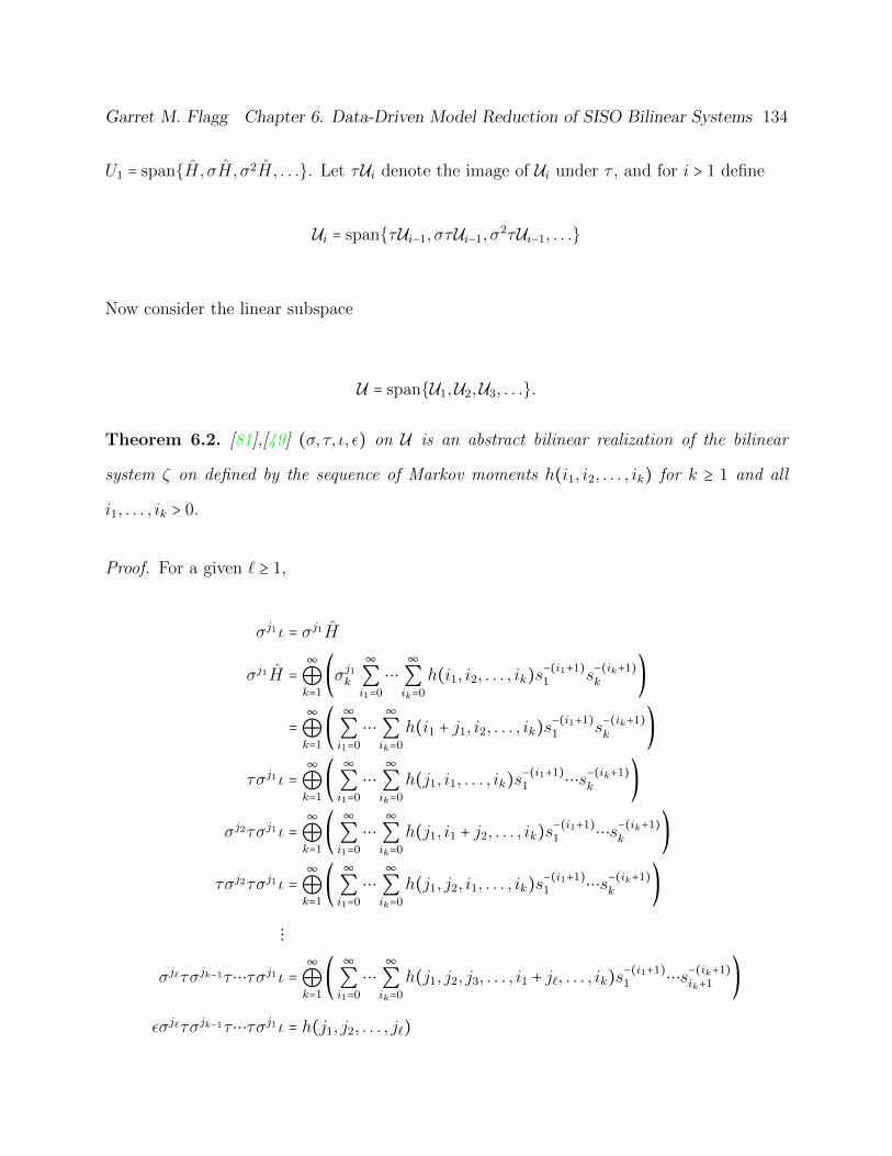
Garret M. Flagg Chapter 6. Data-Driven Model Reduction of SISO Bilinear Systems 134
U1 = span{H, σH, σ2H, . . .}. Let τUi denote the image of Ui under τ , and for i > 1 define
Ui = span{τUi−1, στUi−1, σ2τUi−1, . . .}
Now consider the linear subspace
U = span{U1,U2,U3, . . .}.
Theorem 6.2. [81],[49] (σ, τ, ι, ε) on U is an abstract bilinear realization of the bilinear
system ζ on defined by the sequence of Markov moments h(i1, i2, . . . , ik) for k ≥ 1 and all
i1, . . . , ik > 0.
Proof. For a given ` ≥ 1,
σj1ι = σj1H
σj1H =∞
⊕k=1
(σj1k
∞
∑i1=0
⋯∞
∑ik=0
h(i1, i2, . . . , ik)s−(i1+1)1 s
−(ik+1)k )
=∞
⊕k=1
(∞
∑i1=0
⋯∞
∑ik=0
h(i1 + j1, i2, . . . , ik)s−(i1+1)1 s
−(ik+1)k )
τσj1ι =∞
⊕k=1
(∞
∑i1=0
⋯∞
∑ik=0
h(j1, i1, . . . , ik)s−(i1+1)1 ⋯s
−(ik+1)k )
σj2τσj1ι =∞
⊕k=1
(∞
∑i1=0
⋯∞
∑ik=0
h(j1, i1 + j2, . . . , ik)s−(i1+1)1 ⋯s
−(ik+1)k )
τσj2τσj1ι =∞
⊕k=1
(∞
∑i1=0
⋯∞
∑ik=0
h(j1, j2, i1, . . . , ik)s−(i1+1)1 ⋯s
−(ik+1)k )
⋮
σj`τσjk−1τ⋯τσj1ι =∞
⊕k=1
(∞
∑i1=0
⋯∞
∑ik=0
h(j1, j2, j3, . . . , i1 + j`, . . . , ik)s−(i1+1)1 ⋯s
−(ik+1)ik+1 )
εσj`τσjk−1τ⋯τσj1ι = h(j1, j2, . . . , j`)

Garret M. Flagg Chapter 6. Data-Driven Model Reduction of SISO Bilinear Systems 135
Constructing a finite dimensional realization with matrices (A, N , b, c) representing the
action of the operators σ, τ, ι, ε depends on the dimension of U . If U is finite dimensional,
then the H has a finite dimensional bilinear realization of the same dimension. Using this
construction, one can also generalize the Hankel matrix for linear systems to a behavior
matrix for bilinear systems. Identify H, σH, τH and so on with their sequences of Markov
moments
H = ((h(0), h(1), h(2), . . .), (h(0,0), h(0,1), h(0,2), . . . , h(1,0), h(1,1), h(1,2), . . .), . . .)
σH = ((h(1), h(2), h(3), . . .), (h(1,0), h(1,1), h(1,2), . . . , h(2,0), h(2,1), h(2,2), . . .), . . .)
τH = ((h(0,0), h(0,1), h(0,2), . . .), (h(0,0,0), h(0,0,1), h(0,0,2), . . . ,
h(0,1,0), h(0,1,1), h(0,1,2), . . .), . . .)
Through this identification, we can then write

Garret M. Flagg Chapter 6. Data-Driven Model Reduction of SISO Bilinear Systems 136
BH =
⎡⎢⎢⎢⎢⎢⎢⎢⎢⎢⎢⎢⎢⎢⎢⎢⎢⎢⎢⎢⎢⎢⎢⎢⎢⎢⎢⎢⎢⎢⎢⎢⎢⎢⎣
H
σH
σ2H
⋮
τH
στH
σ2τH
⋮
σj`τ⋯τσj1H
⎤⎥⎥⎥⎥⎥⎥⎥⎥⎥⎥⎥⎥⎥⎥⎥⎥⎥⎥⎥⎥⎥⎥⎥⎥⎥⎥⎥⎥⎥⎥⎥⎥⎥⎦
=
⎡⎢⎢⎢⎢⎢⎢⎢⎢⎢⎢⎢⎢⎢⎢⎢⎢⎢⎣
h(0) h(1) . . . h(0,0) h(0,1) . . .
h(1) h(2) . . . h(1,0) h(1,1) . . .
⋮ ⋮ ⋮ ⋮ ⋮ ⋮
h(0,0) h(0,1) . . . h(0,0,0) h(0,0,1) . . .
⋮ ⋮ ⋮ ⋮ ⋮ ⋮
⎤⎥⎥⎥⎥⎥⎥⎥⎥⎥⎥⎥⎥⎥⎥⎥⎥⎥⎦
There are many ways to systematically list the sequences in the Markov moments, and so the
behavior matrix given above is a nonunique description of H. Isidori et. al. [59] constructed
an alternative behavior matrix and used it to construct a bilinear realization directly, without
any discussion of shift operators. The entries of their matrix, properly reordered, correspond
to the BH as it is presented here.
6.2 The structure of the interpolation data
The solution of the interpolation problem posed on the kth order Volterra kernels presented
in Theorem 3.2 provides insight into a natural way to organize the interpolation data. In
effect, all the interpolation data is essentially determined by the highest order subsystem
for which interpolation conditions are stipulated. Assume that the subsystem of order N
is the highest order subsystem for which interpolation constraints are imposed. Similar to
the construction of the Krylov subspaces in Theorem 3.2, we build the notation for the
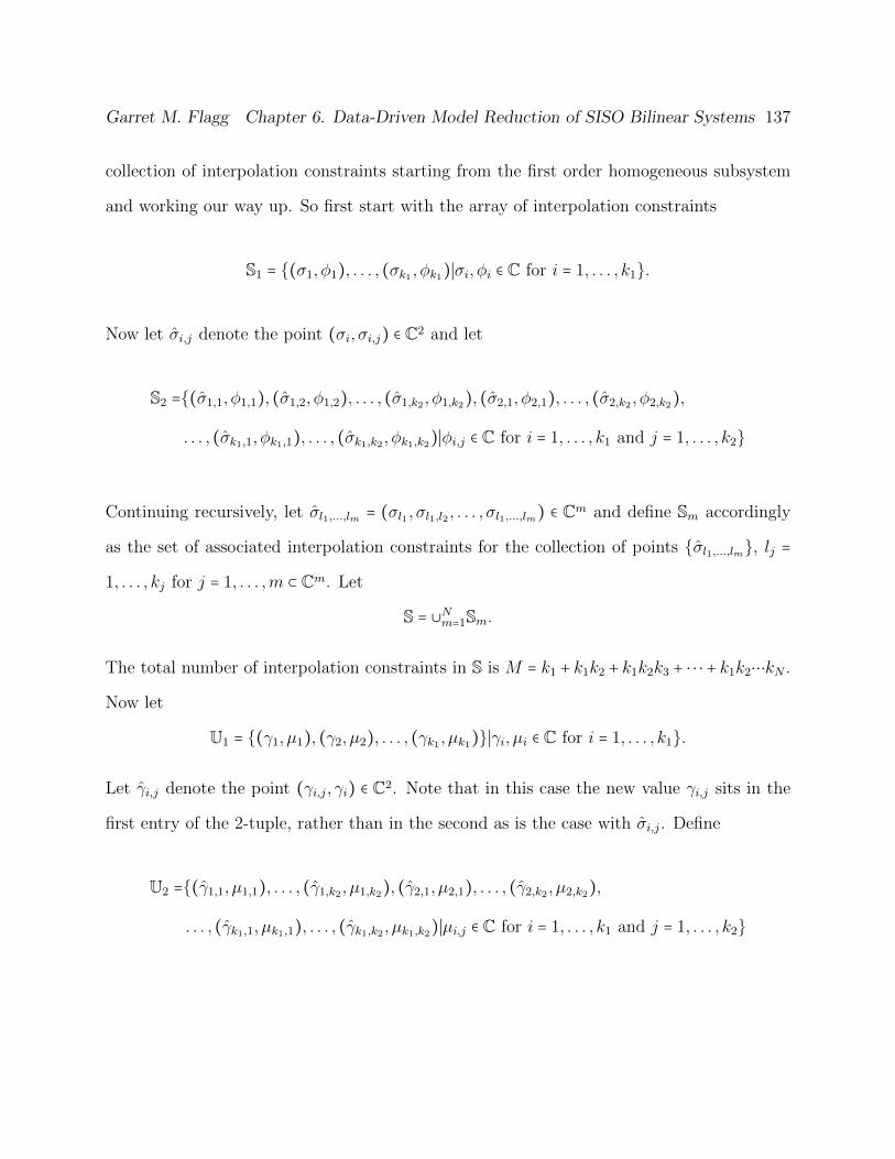
Garret M. Flagg Chapter 6. Data-Driven Model Reduction of SISO Bilinear Systems 137
collection of interpolation constraints starting from the first order homogeneous subsystem
and working our way up. So first start with the array of interpolation constraints
S1 = {(σ1, φ1), . . . , (σk1 , φk1)∣σi, φi ∈ C for i = 1, . . . , k1}.
Now let σi,j denote the point (σi, σi,j) ∈ C2 and let
S2 ={(σ1,1, φ1,1), (σ1,2, φ1,2), . . . , (σ1,k2 , φ1,k2), (σ2,1, φ2,1), . . . , (σ2,k2 , φ2,k2),
. . . , (σk1,1, φk1,1), . . . , (σk1,k2 , φk1,k2)∣φi,j ∈ C for i = 1, . . . , k1 and j = 1, . . . , k2}
Continuing recursively, let σl1,...,lm = (σl1 , σl1,l2 , . . . , σl1,...,lm) ∈ Cm and define Sm accordingly
as the set of associated interpolation constraints for the collection of points {σl1,...,lm}, lj =
1, . . . , kj for j = 1, . . . ,m ⊂ Cm. Let
S = ∪Nm=1Sm.
The total number of interpolation constraints in S is M = k1 + k1k2 + k1k2k3 + ⋅ ⋅ ⋅ + k1k2⋯kN .
Now let
U1 = {(γ1, µ1), (γ2, µ2), . . . , (γk1 , µk1)}∣γi, µi ∈ C for i = 1, . . . , k1}.
Let γi,j denote the point (γi,j, γi) ∈ C2. Note that in this case the new value γi,j sits in the
first entry of the 2-tuple, rather than in the second as is the case with σi,j. Define
U2 ={(γ1,1, µ1,1), . . . , (γ1,k2 , µ1,k2), (γ2,1, µ2,1), . . . , (γ2,k2 , µ2,k2),
. . . , (γk1,1, µk1,1), . . . , (γk1,k2 , µk1,k2)∣µi,j ∈ C for i = 1, . . . , k1 and j = 1, . . . , k2}

Garret M. Flagg Chapter 6. Data-Driven Model Reduction of SISO Bilinear Systems 138
Define the sets Um for m = 3, . . .N similarly to U2, and let
U = ∪Nm=1Um.
There are also M = k1 + k1k2 + k1k2k3 + ⋅ ⋅ ⋅ + k1k2⋯kN interpolation constraints in U. A last
collection of interpolation constraints is needed to determine the N matrix in the bilinear
realization. Let
σ = [σ1, . . . , σk1 , σ1,1, . . . , σ1,k2 , σ2,1, . . . , σ2,k2 , . . . , σ1,1,...,1, σ1,1,...,2, . . . , σ1,1,...,kN , . . . , σk1,k2,...,kN ]
be a row vector of length M that uniquely lists the whole collection of values enumerated
in the m − tuples defined in Sm m = 1, . . . ,N . Let γ similarly be a row vector of length
M that lists all the values in the m − tuples given by the arrays Um for m = 1, . . . ,N .
Let C = σ ⊗ γ be the tensor product of σ and γ, and with each entry σl1,...,lm ⊗ γr1,...,ru
for m,u = 1, . . . ,N and lm = 1, . . . , km, ru = 1, . . . , ku of the tensor identify the point
(σl1 , σl1,l2 , . . . , σl1,...,lm , γl1,...,lu , γl1,...,lu−1 , . . . , γl1) ∈ Cm+u. Define the last collection of inter-
polation constraints as
T = {(σl1,...,lm ⊗ γr1,...,ru , η(l1,...,lm),(r1,...,ru))∣(σl1,...,lm ⊗ γr1,...,ru) ∈ Cm+u and η(l1,...,lm),(r1,...,ru) ∈ C}
(6.4)
Let
P = S ∪U ∪T. (6.5)
The total number of interpolation constraints stipulated in P is 2M +M2, where again
M = k1 + k1k2 + k1k2k3 + ⋅ ⋅ ⋅ + k1k2⋯kN . We will encode the data corresponding to point con-
catenations in T in a concatenation matrix denoted by τL. First, we place the interpolation

Garret M. Flagg Chapter 6. Data-Driven Model Reduction of SISO Bilinear Systems 139
values η(l1,...,lm),(r1,...,ru) in a long column matrix denoted η in the same order as the entries
of the tensor σ⊗γ. Partition η into M blocks of length M denoted ηi for i = 1, . . . ,M as in
η = [η1 η2 . . . ηM] ∈ C1×M2
(6.6)
Each ηi collects all the interpolation constraints for some point σr1,...,ru concatenated with
each of the points in γ. Now define
τL = [vec(η1) vec(η2) . . . vec(ηM)] ∈ CM×M (6.7)
6.3 Construction of the Bilinear Realization
In order to obtain the bilinear realization, we first use S and U to construct a MIMO linear
realization satisfying tangential interpolation constraints determined by S and U. For the
given data, a MIMO system having q = 1 + k1 + k1k2 + k1k2k3 + ⋅ ⋅ ⋅ + k1k2⋯kN−1 inputs and
outputs will be constructed. Thus, we must first translate the data in S, and U into right
and left tangential interpolation conditions respectively. Let Iq be the identity in Rq×q, and
let the vectors ej for j = 1, . . . , q denote the jth column of the identity. With each pair
(γl1,...,lm , µl1,...,lm) ∈ U associate the tuple (γl1,...,lm ,vMm+Ll1,...,lm, lMm+Ll1,...,lm
= eTJm+Ll1,...,lm−1
),
where
J1 = 0, J2 = 1, and Jm =m
∑j=1
Jlj + k1k2⋯km−2 for m > 2, (6.8)
M1 = 0 and Mm =m
∑j=1
Mj + k1k2⋯km−1, for m > 1 (6.9)
(6.10)

Garret M. Flagg Chapter 6. Data-Driven Model Reduction of SISO Bilinear Systems 140
Ll1,...,lm = 1, . . . , k1k2⋯km uniquely enumerates the combinations l1, . . . , lm by first running
through the indices in lm and fixing all the other indices at one, then incrementing the index
in lm−1 by one and lm and keeping l1, . . . , lm−2 fixed and so on. Let
vMm+Ll1,...,lm= [µl1,...,lm , τL(Mm +Ll1,...,lm ,1 ∶MN)] ∈ Cq.
Define the whole collection of left interpolation conditions by
M = diag(γ) ∈ CM×M
L = [lT1 , . . . , lTM]T ∈ CM×q and V =
⎡⎢⎢⎢⎢⎢⎢⎢⎢⎢⎣
v1
⋮
vM
⎤⎥⎥⎥⎥⎥⎥⎥⎥⎥⎦
∈ CM×q.
(6.11)
Next, we construct right tangential interpolation conditions from S. Again for each pair
(σl1,...,lm , φl1,...,lm) associate the tuple (σl1,...,lm ,wMm+Ll1,...,lm,rMm+Ll1,...,lm
= eJm+Ll1,...,lm−1
), where
here
wMm+Ll1,...,lm=
⎡⎢⎢⎢⎢⎢⎢⎣
φl1,...,lm
τL(1 ∶MN ,Mm +Ll1,...,lm)
⎤⎥⎥⎥⎥⎥⎥⎦
(6.12)
Define the full collection of right interpolation conditions by

Garret M. Flagg Chapter 6. Data-Driven Model Reduction of SISO Bilinear Systems 141
Λ = diag(σ) ∈ CM×M
R = [r1, . . . ,rM], and W = [w1, . . . ,wM] ∈ Cq×M .
(6.13)
From this data, the Loewner matrix and shifted Loewner matrices L and σL can be con-
structed as the solutions of the following Lyapunov equations [70]:
LΛ −ML = LW −V R σLΛ −MσL = LWΛ −MVR (6.14)
Assume that for some k ≤M assumption (6.1) is satisfied. Then construct the linear system
Σ=(A ∈ Ck×k, B ∈ Ck×p, C ∈ Cp×k, 0 ∈ Cp×p) according to Theorem 6.1. In order to construct
a bilinear realization, we make the following additional assumptions on the data:
Assumption: Either k =M or k = p and rank(L(1 ∶ k,1 ∶ k)) = k (6.15)
Assuming either case in assumption (6.15) holds, a bilinear system realization (A,N , b, c)
which will satisfy all the interpolation conditions given in P can be constructed directly from
(A, B, C) and the data in τL.
To complete the construction of a bilinear realization, we need to extract some additional in-
formation from the matrix τL to constructN . We break the development of the construction
into the two possible cases k =M or k = p.
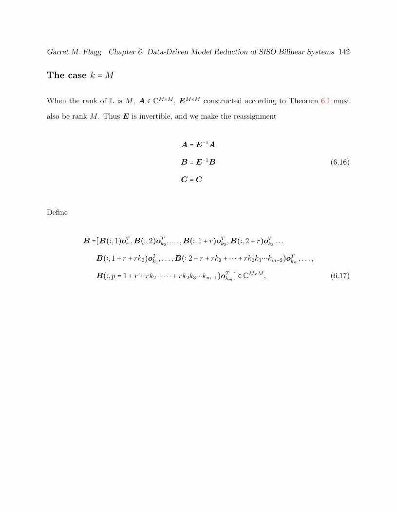
Garret M. Flagg Chapter 6. Data-Driven Model Reduction of SISO Bilinear Systems 142
The case k =M
When the rank of L is M , A ∈ CM×M , EM×M constructed according to Theorem 6.1 must
also be rank M . Thus E is invertible, and we make the reassignment
A =E−1A
B =E−1B (6.16)
C =C
Define
B =[B(∶,1)oTr ,B(∶,2)oTk2 , . . . ,B(∶,1 + r)oTk2 ,B(∶,2 + r)oTk3 . . .
B(∶,1 + r + rk2)oTk3, . . . ,B(∶ 2 + r + rk2 + ⋅ ⋅ ⋅ + rk2k3⋯km−2)o
Tkm, . . . ,
B(∶, p = 1 + r + rk2 + ⋅ ⋅ ⋅ + rk2k3⋯km−1)oTkm
] ∈ CM×M , (6.17)

Garret M. Flagg Chapter 6. Data-Driven Model Reduction of SISO Bilinear Systems 143
C =
⎡⎢⎢⎢⎢⎢⎢⎢⎢⎢⎢⎢⎢⎢⎢⎢⎢⎢⎢⎢⎢⎢⎢⎢⎢⎢⎢⎢⎢⎢⎢⎢⎢⎢⎢⎢⎢⎢⎢⎢⎢⎣
orC(1, ∶)
ok2C(2, ∶)
⋮
ok2C(r + 1, ∶)
ok3C(r + 2, ∶)
⋮
ok3C(1 + r + k2r, ∶)
⋮
okmC(2 + r + rk2 + ⋅ ⋅ ⋅ + rk2k3⋯km−2, ∶)
⋮
okmC(∶, p = 1 + r + rk2 + ⋅ ⋅ ⋅ + rk2k3⋯km−1)
⎤⎥⎥⎥⎥⎥⎥⎥⎥⎥⎥⎥⎥⎥⎥⎥⎥⎥⎥⎥⎥⎥⎥⎥⎥⎥⎥⎥⎥⎥⎥⎥⎥⎥⎥⎥⎥⎥⎥⎥⎥⎦
∈ CM×M (6.18)
Now let U , QT ∈ CM×M be the solutions of
UΛ −AU − B = 0 QTM −AT QT − CT = 0 (6.19)
The matrices U and Q provide a factorization of the Loewner matrix L.
Theorem 6.3. Let L ∈ CM×M be the Loewner matrix formed from the interpolation data Λ,
R,W ,M ,L,V , and assume that rank(L) =M . Then L = −QU .
Remark 6.1. From the assumption that L is full rank, it follows from Theorem 6.3 that Q
and U are full rank and therefore invertible.
Proof. Let {xi,j} =QU and {li,j} = L. Let qi be the ith row of Q and let uj be the jth row of
U for i, j = 1, . . . ,M . By the construction of Q, and U , the ith row of Q corresponds to the
row vector C(i, ∶)(γl1,...,lmI −A)−1, for some γl1,...,lm corresponding to the entry M(i, i) and
by the construction of C, C(∶, i) = C(∶, Jlm−1 + Ll1,...,lm−1). Likewise, uj corresponds to the
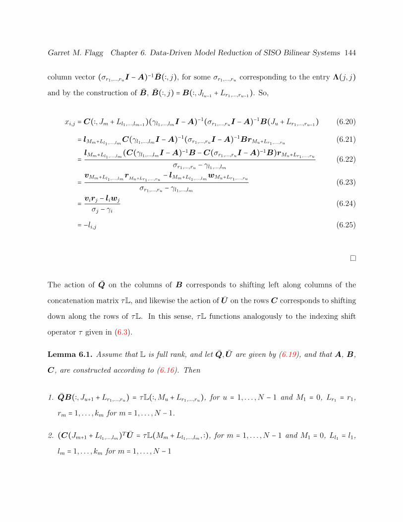
Garret M. Flagg Chapter 6. Data-Driven Model Reduction of SISO Bilinear Systems 144
column vector (σr1,...,ruI −A)−1B(∶, j), for some σr1,...,ru corresponding to the entry Λ(j, j)
and by the construction of B, B(∶, j) =B(∶, Jlu−1 +Lr1,...,ru−1). So,
xi,j =C(∶, Jm +Ll1,...,lm−1)(γl1,...,lmI −A)−1(σr1,...,ruI −A)−1B(Ju +Lr1,...,ru−1) (6.20)
= lMm+Ll1,...,lmC(γl1,...,lmI −A)−1(σr1,...,ruI −A)−1BrMu+Lr1,...,ru
(6.21)
=lMm+Ll1,...,lm
(C(γl1,...,lmI −A)−1B −C(σr1,...,ruI −A)−1B)rMu+Lr1,...,ru
σr1,...,ru − γl1,...,lm(6.22)
=vMm+Ll1,...,lm
rMu+Lr1,...,ru
− lMm+Ll1,...,lmwMu+Lr1,...,ru
σr1,...,ru − γl1,...,lm(6.23)
=virj − liwj
σj − γi(6.24)
= −li,j (6.25)
The action of Q on the columns of B corresponds to shifting left along columns of the
concatenation matrix τL, and likewise the action of U on the rows C corresponds to shifting
down along the rows of τL. In this sense, τL functions analogously to the indexing shift
operator τ given in (6.3).
Lemma 6.1. Assume that L is full rank, and let Q, U are given by (6.19), and that A, B,
C, are constructed according to (6.16). Then
1. QB(∶, Ju+1 +Lr1,...,ru) = τL(∶,Mu +Lr1,...,ru), for u = 1, . . . ,N − 1 and M1 = 0, Lr1 = r1,
rm = 1, . . . , km for m = 1, . . . ,N − 1.
2. (C(Jm+1 +Ll1,...,lm)T U = τL(Mm +Ll1,...,lm , ∶), for m = 1, . . . ,N − 1 and M1 = 0, Ll1 = l1,
lm = 1, . . . , km for m = 1, . . . ,N − 1

Garret M. Flagg Chapter 6. Data-Driven Model Reduction of SISO Bilinear Systems 145
Proof. Fix some r1, . . . , ru. For i = 1, . . . ,M
Q(i, ∶)B(∶, Ju+1 +Lr1,...,ru) = C(i, ∶)(γl1,...,lmI −A)BeJu+1+Lr1,...,ru
(6.26)
=C(Jm +Ll1,...,lm−1 , ∶)(γl1,...,lm)I −A)−1BeJu+1+Lr1,...,ru
(6.27)
= lMm+Ll1,...,lmC(γl1,...,lmI −A)−1Be
Ju+1+Lr1,...,ru(6.28)
= vMm+Ll1,...,lm(Ju+1 +Lr1,...,ru) (6.29)
= τL(Mm +Ll1,...,lm ,Mu +Lr1,...,ru) (6.30)
Since each row i =Mm +Ll1,...,lm of Q corresponds to some point γl1,...,lm , the product of the
rows of Q with the column B(∶, Ju+1 +Lr1,...,ru) corresponds to concatenating all the points
in γ with the point σr1,...,ru . By the definition of τL, this is the same thing as the column
τL(∶,Mu +Lr1,...,ru). This proves 1.
For the proof of 2., fix some l1, . . . , lm. Then for j = 1, . . . ,M
C(∶, Jm+1 +Ll1,...,lm)U(∶, j) =C(∶, Jm+1 +Ll1,...,lm)(σr1,...,ruI −A)−1B(∶, j) (6.31)
(from the definition of B).
= eTJm+1+Ll1,...,lmC(σr1,...,ruI −A)−1B(∶, Ju +Lr1,...,ru−1),
= eTJm+1+Ll1,...,lmC(σr1,...,ruI −A)−1BrMu+Lr1,...,ru
(6.32)
=wMu+Lr1,...,ru(Jm+1 +Ll1,...,lm) (6.33)
= τL(Mm +Ll1,...,lm ,Mu +Lr1,...,ru) (6.34)
Since each column j =Mu+Lr1,...,ru of U corresponds to the point σr1,...,ru , the product of the
columns of U with the row C(∶, Jm+1 +Ll1,...,lm) corresponds to concatenating all the points
in σ with the point γl1,...,lm , which is equivalent to (6.34).
Garret M. Flagg Chapter 6. Data-Driven Model Reduction of SISO Bilinear Systems 146
We now have all the components necessary to construct the bilinear realization. Define
b =B(∶,1) (6.35)
c =C(1, ∶) (6.36)
N = Q−1τLU−1. (6.37)
Theorem 6.4. Given the interpolation constraints P defined in (6.5), assume that rank(L) =
M and let A, B, C be defined as in (6.16), U , Q be given by (6.19), and b, c, N be
given by (6.35), (6.36), (6.37) respectively. Then ζ:=(A,N ,b,c) satisfies all the subsystem
interpolation conditions in the array P.
Proof. We first consider the case where the interpolation constraint is in the array S. Suppose
we have the pair (σr1,...,ru , φr1,...,ru) ∈ S. Then
Hu(σr1 , σr1,r2 , . . . , σr1,...,ru)
=c(σr1,...,ruI −A)−1N(σr1,...,ru−1I −A)−1N⋯N(σr1,r2I −A)−1N(σr1I −A)−1b
=c(σr1,...,ruI −A)−1N(σr1,...,ru−1I −A)−1N⋯N(σr1,r2I −A)−1Q−1τLU−1U(∶, r1)
=c(σr1,...,ruI −A)−1N(σr1,...,ru−1I −A)−1N⋯N(σr1,r2I −A)−1Q−1τLM1+r1
(By Lemma 6.2) (6.38)
=c(σr1,...,ruI −A)−1N(σr1,...,ru−1I −A)−1N⋯N(σr1,r2I −A)−1Q−1QB(∶, J2 +Lr1)
=c(σr1,...,ruI −A)−1N(σr1,...,ru−1I −A)−1N⋯N(σr1,r2I −A)−1B(∶, J2 +Lr1)
=c(σr1,...,ruI −A)−1N(σr1,...,ru−1I −A)−1N⋯N(σr1,r2I −A)−1B(∶,Mr2 +Lr2)
=c(σr1,...,ruI −A)−1N(σr1,...,ru−1I −A)−1N⋯(σr1,r2,...,r3I −A)−1NU(∶,Mr2 +Lr2)
=c(σr1,...,ruI −A)−1N(σr1,...,ru−1I −A)−1N⋯(σr1,r2,...,r3I −A)−1Q−1τLU−1U(∶,Mr2 +Lr2)
Then by Lemma 6.2)

Garret M. Flagg Chapter 6. Data-Driven Model Reduction of SISO Bilinear Systems 147
=c(σr1,...,ruI −A)−1N(σr1,...,ru−1I −A)−1N⋯(σr1,r2,...,r3I −A)−1Q−1QB(∶, Jr3 +Lr2)
⋮ (Reapplying Lemma 6.2 at each step)
=c(σr1,...,ruI −A)−1NUMu−1+Lr1,...,ru−1
=c(σr1,...,ruI −A)−1Q−1τLU−1UMu−1+Lr1,...,ru−1
=c(σr1,...,ruI −A)−1Q−1QB(∶, Ju +Lr1,...,ru−1)
=c(σr1,...,ruI −A)−1B(∶, Ju +Lr1,...,ru−1)
=eT1C(σr1,...,ruI −A)−1BrMu+Lr1,...,ru
=eT1wMu+Lr1,...,ru
=φr1,...,ru (6.39)
A proof for every interpolation constraint in U follows similarly, also using Lemma 6.2. Recall
that for a pair (σr1,...,ru ⊗ γl1,...,lm , η(r1,...,ru),(l1,...,lm)) ∈ T, σr1,...,ru ⊗ γl1,...,lm corresponds to the
point
(σr1 , σr1,r2 , . . . , σr1,...,ru , γl1,...,lm , γl1,...,lm−1 , . . . , γl1) ∈ Cm+u,
and η(r1,...,ru),(l1,...,lm) is the value of the subsystem Hu+m(s1, . . . , su+m) evaluated at this point.
By the first part of the proof note that
Hu+m(σr1,...,ru ⊗ γl1,...,lm)
=C(Jm +Ll1,...,lm−1 , ∶)(γl1,...,lmI −A)−1N(σr1,...,ruI −A)−1B(Ju +Lr1,...,ru−1)
=Q(Mm +Ll1,...,lm , ∶)Q−1τLU−1U(∶,Mu +Lr1,...,ru)
=eTMm+Ll1,...,lmτLeMu+Ll1,...,lu
=τL(Mm +Ll1,...,lm ,Mu +Lr1,...,ru)
=η(r1,...,ru),(l1,...,lm) (6.40)

Garret M. Flagg Chapter 6. Data-Driven Model Reduction of SISO Bilinear Systems 148
The case k = q and rank(L(1 ∶ q,1 ∶ q)) = q
Now we will assume that rank(L) = q <M , and rank(L(1 ∶ q,1 ∶ q)) = q. In this case,A ∈ Cq×q,
E constructed according to Theorem 6.1 must also be rank q. Thus E is invertible, and we
make the reassignment
A =E−1A
B =E−1B (6.41)
C =C
but L ∈ CM×M , so to construct a bilinear realization with conformable dimensions, we will
make use of the information in the submatrix τL(1 ∶ q,1 ∶ q) and the submatrix L(1 ∶ q,1 ∶ q).
First let U , Q∈ Cq×q solve
UΛ(1 ∶ q,1 ∶ q) −AU −B = 0 QTM(1 ∶ q,1 ∶ q) −ATQT −CT = 0 (6.42)
The matrices U , and Q, are a factorization of L(1 ∶ q,1 ∶ q).
Theorem 6.5. Let L ∈ CM×M be the Loewner matrix formed from the interpolation data Λ,
R,W ,M ,L,V , and assume that rank(L) = q <M . Then L(1 ∶ q,1 ∶ q) = −QU .
Remark 6.2. From the assumption that rank(L(1 ∶ q,1 ∶ q) = q, it follows from Theorem
6.3 that Q and U are full rank and therefore invertible.
Proof. Let {xi,j} = QU and {li,j} = L(1 ∶ q,1 ∶ q) for i, j = 1, . . . , q. Let qi be the ith
row of Q and let uj be the jth row of U for i, j = 1, . . . , q. By the construction of Q,

Garret M. Flagg Chapter 6. Data-Driven Model Reduction of SISO Bilinear Systems 149
and U , the ith row of Q corresponds to the row vector C(i, ∶)(γl1,...,lmI −A)−1, for some
γl1,...,lm corresponding to the entry M(i, i). There is a one-to-one correspondence between
the indices i and the indices Jm + Ll1,...,lm for m = 1, . . . ,N − 1 and lm = 1 . . . , km. So we
can write C(∶, i) = C(∶, Jm + Ll1,...,lm−1). Likewise, uj corresponds to the column vector
(σr1,...,ruI−A)−1B(∶, j), for some σr1,...,ru corresponding to the entry Λ(j, j) and using the fact
that there is a one-to-one correspondence between the indices j and the indices Ju+Lr1,...,ru−1
for u = 1, . . . ,N − 1 and ru = 1, . . . ku, B(∶, j) =B(∶, Ju +Lr1,...,ru−1). So,
xi,j =C(∶, Jm +Ll1,...,lm−1)(γl1,...,lmI −A)−1(σr1,...,ruI −A)−1B(Ju +Lr1,...,ru−1) (6.43)
= lMm+Ll1,...,lmC(γl1,...,lmI −A)−1(σr1,...,ruI −A)−1BrMu+Lr1,...,ru
(6.44)
=lMm+Ll1,...,lm
(C(γl1,...,lmI −A)−1B −C(σr1,...,ruI −A)−1B)rMu+Lr1,...,ru
σr1,...,ru − γl1,...,lm(6.45)
=vMm+Ll1,...,lm
rMu+Lr1,...,ru
− lMm+Ll1,...,lmwMu+Lr1,...,ru
σr1,...,ru − γl1,...,lm(6.46)
=virj − liwj
σj − γi(6.47)
= li,j (6.48)
As in Lemma 6.2, the following lemma connects the concatenation matrix τL with the action
of U and Q on B, and C respectively.
Lemma 6.2. Assume that L(1 ∶ q,1 ∶ q) is full rank, and let Q,U be given by (6.42). Let
A, B, Cbe given by (6.41). Then
1. QB(∶, Ju+1 +Lr1,...,ru) = τL(∶,Mu +Lr1,...,ru), for u = 1, . . . ,N − 1 and M1 = 0, Lr1 = r1,
rm = 1, . . . , km for m = 1, . . . ,N − 1.
2. (C(Jm+1 +Ll1,...,lm)TU = τL(Mm +Ll1,...,lm , ∶), for m = 1, . . . ,N − 1 and M1 = 0, Ll1 = l1,

Garret M. Flagg Chapter 6. Data-Driven Model Reduction of SISO Bilinear Systems 150
lm = 1, . . . , km for m = 1, . . . ,N − 1
Proof. The proof is exactly the same as in the proof of Lemma 6.2, except the bars are
removed from all the obvious quantities.
We now have all the components necessary to construct the bilinear realization. Define
b =B(∶,1) (6.49)
c =C(1, ∶) (6.50)
N =Q−1τLU−1. (6.51)
Theorem 6.6. Given the interpolation constraints P defined in (6.5), assume that rank(L) =
q and let A, B, C be defined as in (6.41), U , Q be given by (6.42), and b, c, N be
given by (6.49), (6.50), (6.51) respectively. Then ζ:=(A,N ,b,c) satisfies all the subsystem
interpolation conditions in the array P.
Proof. The proof is the same as in Theorem 6.4, except all the bars are dropped from the
obvious quantities.
The following algorithm summarizes the approach for constructing a bilinear system that
interpolates the data.
Algorithm 6.1 (Bilinear realization from transfer function data).
Input: P = T ∪ S ∪U
Output: A,N ,b,c
1. Construct the matrices σ, γ, and η
τL = [η1, . . . , ηk1 , η1,1, η1,2, . . . , η1,k2 , η2,1, . . . , ηk1,k2 , . . . , η2,1 , . . . , ηk1,...,kN ] from S, U, T.

Garret M. Flagg Chapter 6. Data-Driven Model Reduction of SISO Bilinear Systems 151
2. Λ = diag(σ), M = diag(γ), R = [eJm+Ll1,...,lm−1 ], for m = 1, . . . ,N and lm = 1, . . . , km.
L =RT
3. For m = 1, . . . ,N and for lm = 1, . . . , km
V = [V ;µl1,...,lm , τ∗L(Mm +Ll1,...,lm ,1 ∶MN)] (6.52)
W = [W , φl1,...,lm , τL(1 ∶MN ,Mm +Ll1,...,lm)] (6.53)
4. Solve
LΛ −ML = LW −V R σLΛ −MσL = LWΛ −MVR (6.54)
5. Compute
λ1,1L − σL = Y ΣX
where rank(λ1,1L − σL) = rank(Σ) = size(Σ) = k and Y , ∈ Cν×k, X ∈ Ck×ρ.
6. E = −Y ∗LX∗, A =E−1(−Y ∗σLX∗), B =E−1(Y ∗V ), C=WX∗.
7. If (rank(L) =M)
a.) Solve
UΛ −AU = B QTM −AT QT = CT
b.) N = Q−1τLU−1, b =B(∶,1), c =C(1, ∶)
8. Else If (rank(L)=q)

Garret M. Flagg Chapter 6. Data-Driven Model Reduction of SISO Bilinear Systems 152
a.) Solve
UΛ(1 ∶ q,1 ∶ q) −AU =B QTM(1 ∶ q,1 ∶ q) −ATQT =CT
b.) N =Q−1τLU−1, b =B(∶,1), c =C(1, ∶)
9. Else
a. Assumption (6.15) is not satisfied, and no bilinear realization can be constructed.
10. Return A, N , b, c
Examples
A few simple examples illustrate the method of Algorithm 6.1.
Example 1
In this example, we reconstruct the bilinear system ζ = (A,N ,b,c) where
A =
⎡⎢⎢⎢⎢⎢⎢⎣
−1 0
0 −2
⎤⎥⎥⎥⎥⎥⎥⎦
N =
⎡⎢⎢⎢⎢⎢⎢⎣
1 1
1 1
⎤⎥⎥⎥⎥⎥⎥⎦
b =
⎡⎢⎢⎢⎢⎢⎢⎣
1
0
⎤⎥⎥⎥⎥⎥⎥⎦
c = [1 2] (6.55)
H1(s1) is sampled at the points H1(0) and H1(1). The second-order transfer function
H2(s1, s2) is sampled at the points σi = (1, i + 1) , and γi = (0, 1i+1) for i = 1, . . . ,4. Thus,
k1 = 1 and k2 = 4. This yields 2M = 2(k1 + k1k2) = 10 left and right interpolation constraints.
The dimension of the input-output space for the MIMO linear system will be q = 1 + k1 = 2.

Garret M. Flagg Chapter 6. Data-Driven Model Reduction of SISO Bilinear Systems 153
The interpolation constraints in S and U and T are
S = {(1,1/2), ((1,2),5/12)), ((1,3),13/40), ((1,4),4/15), ((1/5),19/84)},
U = {(0,1), ((0,1/2),4/3), ((0,1/3),3/2), ((0,1/4),8/5), ((0,1/5),5/3)},
and
T ={((1,0),1), ((1,1/2,0),16/15), ((1,1/3,0),33/28), ((1,1/4,0),56/45), ((1,1/5,0),85/66),
((1,2,0),7/12), ((1,2,1/2,0),38/45), ((1,2,1/3,0),11/16), ((1,2,1/4,0),98/135),
((1,2,1/5,0),595/792), ((1,3,0),9/20), ((1,3,1/2,0),12/25), ((1,3,1/3,0),297/560),
((1,3,1/4,0),14/25), ((1,3,1/5,0),51/88), ((1,4,0),11/30), ((1,4,1/2,0),88/225),
((1,4,1/3,0),121/280), ((1,4,1/4,0),308/675), ((1,4,1/5,0),17/36), ((1,5,0),13/42),
((1,5,1/2,0),104/315), ((1,5,1/3,0),143/392), ((1,5,1/4,0),52/135),
((1,5,1/5,0),1105/2772)} (6.56)

Garret M. Flagg Chapter 6. Data-Driven Model Reduction of SISO Bilinear Systems 154
The matrices σ,γ, and η, are
σ =
⎡⎢⎢⎢⎢⎢⎢⎢⎢⎢⎢⎢⎢⎢⎢⎢⎢⎢⎣
1
2
3
4
5
⎤⎥⎥⎥⎥⎥⎥⎥⎥⎥⎥⎥⎥⎥⎥⎥⎥⎥⎦
T
γ =
⎡⎢⎢⎢⎢⎢⎢⎢⎢⎢⎢⎢⎢⎢⎢⎢⎢⎢⎣
0
1/2
1/3
1/4
1/5
⎤⎥⎥⎥⎥⎥⎥⎥⎥⎥⎥⎥⎥⎥⎥⎥⎥⎥⎦
T
η =
⎡⎢⎢⎢⎢⎢⎢⎢⎢⎢⎢⎢⎢⎢⎢⎢⎢⎢⎢⎢⎢⎢⎢⎢⎢⎢⎢⎢⎢⎢⎢⎢⎢⎢⎢⎢⎢⎢⎢⎢⎢⎢⎢⎢⎢⎢⎢⎢⎢⎢⎢⎢⎢⎢⎢⎢⎢⎢⎢⎢⎢⎢⎢⎢⎢⎢⎢⎢⎢⎢⎢⎢⎢⎢⎢⎢⎢⎢⎢⎢⎢⎢⎢⎢⎢⎢⎢⎢⎢⎢⎢⎢⎢⎢⎢⎢⎣
1
16/15
33/28
56/45
85/66
7/12
28/45
11/16
98/135
595/792
9/20
12/25
297/560
14/25
51/88
11/30
88/225
121/280
308/675
17/36
13/42
104/315
143/392
52/135
407/1021
⎤⎥⎥⎥⎥⎥⎥⎥⎥⎥⎥⎥⎥⎥⎥⎥⎥⎥⎥⎥⎥⎥⎥⎥⎥⎥⎥⎥⎥⎥⎥⎥⎥⎥⎥⎥⎥⎥⎥⎥⎥⎥⎥⎥⎥⎥⎥⎥⎥⎥⎥⎥⎥⎥⎥⎥⎥⎥⎥⎥⎥⎥⎥⎥⎥⎥⎥⎥⎥⎥⎥⎥⎥⎥⎥⎥⎥⎥⎥⎥⎥⎥⎥⎥⎥⎥⎥⎥⎥⎥⎥⎥⎥⎥⎥⎥⎦
T
. (6.57)

Garret M. Flagg Chapter 6. Data-Driven Model Reduction of SISO Bilinear Systems 155
The concatenation matrix τL is
τL =
⎡⎢⎢⎢⎢⎢⎢⎢⎢⎢⎢⎢⎢⎢⎢⎢⎢⎢⎣
1 7/12 9/20 11/30 13/42
16/15 28/45 12/25 88/225 104/315
33/28 11/16 297/560 121/280 143/392
56/45 98/135 14/25 308/675 52/135
85/66 595/792 51/88 17/36 407/1021
⎤⎥⎥⎥⎥⎥⎥⎥⎥⎥⎥⎥⎥⎥⎥⎥⎥⎥⎦
(6.58)
The left and right tangential interpolation conditions are given below:
Λ = diag([1,2,3,4,5]) R =
⎡⎢⎢⎢⎢⎢⎢⎣
1 0 0 0 0
0 1 1 1 1
⎤⎥⎥⎥⎥⎥⎥⎦
W =
⎡⎢⎢⎢⎢⎢⎢⎣
1/2 5/12 13/40 4/15 19/84
1 35/6 9/20 11/30 13/42
⎤⎥⎥⎥⎥⎥⎥⎦
M = diag([0,1/2,1/3,1/4,1/5]) L =
⎡⎢⎢⎢⎢⎢⎢⎢⎢⎢⎢⎢⎢⎢⎢⎢⎢⎢⎣
1 0
0 1
0 1
0 1
0 1
⎤⎥⎥⎥⎥⎥⎥⎥⎥⎥⎥⎥⎥⎥⎥⎥⎥⎥⎦
V =
⎡⎢⎢⎢⎢⎢⎢⎢⎢⎢⎢⎢⎢⎢⎢⎢⎢⎢⎣
1 1
4/3 16/15
3/2 33/28
8/5 56/45
5/3 85/66
⎤⎥⎥⎥⎥⎥⎥⎥⎥⎥⎥⎥⎥⎥⎥⎥⎥⎥⎦
This tangential interpolation data yields
L =
⎡⎢⎢⎢⎢⎢⎢⎢⎢⎢⎢⎢⎢⎢⎢⎢⎢⎢⎣
−1/2 −7/24 −9/40 −11/60 −13/84
−2/3 −29/90 −37/150 −1/5 −53/315
−3/4 −5/14 −153/560 −31/140 −73/392
−4/5 17/45 −13/45 −158/675 −62/315
−5/6 −155/396 −79/264 −8/33 −565/2772
⎤⎥⎥⎥⎥⎥⎥⎥⎥⎥⎥⎥⎥⎥⎥⎥⎥⎥⎦
(6.59)

Garret M. Flagg Chapter 6. Data-Driven Model Reduction of SISO Bilinear Systems 156
σL =
⎡⎢⎢⎢⎢⎢⎢⎢⎢⎢⎢⎢⎢⎢⎢⎢⎢⎢⎣
1/2 5/12 13/40 4/15 19/84
2/3 19/45 49/150 4/15 71/315
3/4 13/28 201/560 41/140 97/392
4/5 22/45 17/45 208/675 82/315
5/6 50/99 103/264 7/22 745/2772
⎤⎥⎥⎥⎥⎥⎥⎥⎥⎥⎥⎥⎥⎥⎥⎥⎥⎥⎦
(6.60)
and rank(L) = rank(σL) = 2. One can easily check that assumption (6.1) is satisfied for
k = 2. Thus, we construct the linear system E ∈ R2×2, A ∈ R2×2, B ∈ R2×2 and C ∈ R2×2
according to Theorem 6.1 that satisfies all the tangential interpolation constraints. E is
invertible, so we give the realization parameters A←E−1A, B ←E−1B, C below:
A =
⎡⎢⎢⎢⎢⎢⎢⎣
−4399/3742 931/4489
506/725 −6827/3742
⎤⎥⎥⎥⎥⎥⎥⎦
B =
⎡⎢⎢⎢⎢⎢⎢⎣
2231/1462 2215/1514
571/442 −2141/1002
⎤⎥⎥⎥⎥⎥⎥⎦
C =
⎡⎢⎢⎢⎢⎢⎢⎣
1825/2307 −229/1428
221/166 −321/13126
⎤⎥⎥⎥⎥⎥⎥⎦
The state-space transformation
T =
⎡⎢⎢⎢⎢⎢⎢⎣
2231/1462 8809/6292
571/442 −2727/490
⎤⎥⎥⎥⎥⎥⎥⎦
applied to this realization gives
A =
⎡⎢⎢⎢⎢⎢⎢⎣
−1 0
0 −2
⎤⎥⎥⎥⎥⎥⎥⎦
B =
⎡⎢⎢⎢⎢⎢⎢⎣
1 1/2
0 1/2
⎤⎥⎥⎥⎥⎥⎥⎦
C =
⎡⎢⎢⎢⎢⎢⎢⎣
1 2
2 2
⎤⎥⎥⎥⎥⎥⎥⎦
The tangential interpolation data falls into the case where the rank(L) = 2 = q, the number

Garret M. Flagg Chapter 6. Data-Driven Model Reduction of SISO Bilinear Systems 157
of inputs, and rank(L(1 ∶ q,1 ∶ q)) = 2. Hence to find N , we solve
UΛ(1 ∶ 2,1 ∶ 2) −AU =B QTM(1 ∶ 2,1 ∶ 2) −ATQT =CT
for U , and Q. This gives
U =
⎡⎢⎢⎢⎢⎢⎢⎣
1/2 1/6
0 1/8
⎤⎥⎥⎥⎥⎥⎥⎦
Q =
⎡⎢⎢⎢⎢⎢⎢⎣
1 1
4/3 4/5
⎤⎥⎥⎥⎥⎥⎥⎦
,
and therefore
N =Q−1τL(1 ∶ 2,1 ∶ 2)U−1 =
⎡⎢⎢⎢⎢⎢⎢⎣
1 1
1 1
⎤⎥⎥⎥⎥⎥⎥⎦
Thus, we assign b =
⎡⎢⎢⎢⎢⎢⎢⎣
1
0
⎤⎥⎥⎥⎥⎥⎥⎦
=B(∶,1) and c = [1 2] =C(1, ∶) and recover the bilinear realization
A =
⎡⎢⎢⎢⎢⎢⎢⎣
−1 0
0 −2
⎤⎥⎥⎥⎥⎥⎥⎦
N =
⎡⎢⎢⎢⎢⎢⎢⎣
1 1
1 1
⎤⎥⎥⎥⎥⎥⎥⎦
b =
⎡⎢⎢⎢⎢⎢⎢⎣
1
0
⎤⎥⎥⎥⎥⎥⎥⎦
c = [1 2] (6.61)
In this example, it was possible to reconstruct the bilinear system ζ exactly from the data.
Our goal was basically to construct the linear MIMO system with realization
A =
⎡⎢⎢⎢⎢⎢⎢⎣
−1 0
0 −2
⎤⎥⎥⎥⎥⎥⎥⎦
B = [b N(I −A)−1b] C =
⎡⎢⎢⎢⎢⎢⎢⎣
c
c(0I −A)−1N
⎤⎥⎥⎥⎥⎥⎥⎦
The system with this realization had exactly 10 free parameters, and we stipulated 10 linearly
independent tangential interpolation conditions, so we were able to construct exactly this
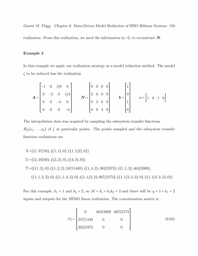
Garret M. Flagg Chapter 6. Data-Driven Model Reduction of SISO Bilinear Systems 158
realization. From this realization, we used the information in τL to reconstruct N .
Example 2
In this example we apply our realization strategy as a model reduction method. The model
ζ to be reduced has the realization
A =
⎡⎢⎢⎢⎢⎢⎢⎢⎢⎢⎢⎢⎢⎢⎣
−1 0 1/6 0
0 −2 0 1/4
0 0 −3 0
0 0 0 −4
⎤⎥⎥⎥⎥⎥⎥⎥⎥⎥⎥⎥⎥⎥⎦
N =
⎡⎢⎢⎢⎢⎢⎢⎢⎢⎢⎢⎢⎢⎢⎣
0 0 0 0
2 0 0 0
0 3 0 0
0 0 4 0
⎤⎥⎥⎥⎥⎥⎥⎥⎥⎥⎥⎥⎥⎥⎦
b =
⎡⎢⎢⎢⎢⎢⎢⎢⎢⎢⎢⎢⎢⎢⎣
1
0
1
0
⎤⎥⎥⎥⎥⎥⎥⎥⎥⎥⎥⎥⎥⎥⎦
c = [1 0 1 0]
The interpolation data was acquired by sampling the subsystem transfer functions
Hk(s1, . . . , sk) of ζ at particular points. The points sampled and the subsystem transfer
function evaluations are
S ={(1,37/48), ((1,1),0), ((1,1/2),0)}
U ={(2,49/40), ((2,2),0), ((4,2),0)}
T ={((1,2),0), ((1,2,2),247/1440), ((1,4,2),382/3373), ((1,1,2),463/2009),
((1,1,2,2),0), ((1,1,4,2),0), ((1,1/2,2),667/2173), ((1,1/2,2,2),0), ((1,1/2,4,2),0)}
For this example, k1 = 1 and k2 = 2, so M = k1 + k1k2 = 3 and there will be q = 1 + k1 = 2
inputs and outputs for the MIMO linear realization. The concatenation matrix is
τL =
⎡⎢⎢⎢⎢⎢⎢⎢⎢⎢⎣
0 463/2009 667/2173
247/1440 0 0
382/3373 0 0
⎤⎥⎥⎥⎥⎥⎥⎥⎥⎥⎦
(6.62)

Garret M. Flagg Chapter 6. Data-Driven Model Reduction of SISO Bilinear Systems 159
The left and right interpolation data is
Λ =
⎡⎢⎢⎢⎢⎢⎢⎢⎢⎢⎣
1 0 0
0 1 0
0 0 1/2
⎤⎥⎥⎥⎥⎥⎥⎥⎥⎥⎦
R =
⎡⎢⎢⎢⎢⎢⎢⎣
1 0 0
0 1 1
⎤⎥⎥⎥⎥⎥⎥⎦
W =
⎡⎢⎢⎢⎢⎢⎢⎣
37/48 0 0
0 463/2009 917/3299
⎤⎥⎥⎥⎥⎥⎥⎦
M =
⎡⎢⎢⎢⎢⎢⎢⎢⎢⎢⎣
2 0 0
0 2 0
0 0 4
⎤⎥⎥⎥⎥⎥⎥⎥⎥⎥⎦
L =
⎡⎢⎢⎢⎢⎢⎢⎢⎢⎢⎣
1 0
0 1
0 1
⎤⎥⎥⎥⎥⎥⎥⎥⎥⎥⎦
V =
⎡⎢⎢⎢⎢⎢⎢⎢⎢⎢⎣
49/90 0
0 247/1440
0 382/3373
⎤⎥⎥⎥⎥⎥⎥⎥⎥⎥⎦
This tangential interpolation data gives
L =
⎡⎢⎢⎢⎢⎢⎢⎢⎢⎢⎣
−163/720 0 0
0 −621/10537 −376/5299
0 −79/2022 −405/8606
⎤⎥⎥⎥⎥⎥⎥⎥⎥⎥⎦
, σL =
⎡⎢⎢⎢⎢⎢⎢⎢⎢⎢⎣
229/720 0 0
0 76/675 551/4050
0 356/4799 323/3600
⎤⎥⎥⎥⎥⎥⎥⎥⎥⎥⎦
The rank of L = 3, so this example falls in the case where rank(L) = M . We construct the
linear system E ∈ R3×3, A ∈ R3×3, B ∈ R3×3 and C ∈ R3×3 according to Theorem 6.1 that
satisfies all the tangential interpolation constraints. E is invertible, so we give the realization
parameters A←E−1A, B ←E−1B, C below:
A =
⎡⎢⎢⎢⎢⎢⎢⎢⎢⎢⎣
−229/163 0 0
0 −944/511 83/13260
0 −8399/160 −2122/511
⎤⎥⎥⎥⎥⎥⎥⎥⎥⎥⎦
, B =
⎡⎢⎢⎢⎢⎢⎢⎢⎢⎢⎣
−392/163 0
0 2520/1391
0 8128/217
⎤⎥⎥⎥⎥⎥⎥⎥⎥⎥⎦
,
C =
⎡⎢⎢⎢⎢⎢⎢⎣
−37/48 0 0
0 295/817 65/436442
⎤⎥⎥⎥⎥⎥⎥⎦

Garret M. Flagg Chapter 6. Data-Driven Model Reduction of SISO Bilinear Systems 160
From the realization data we next compute
U =
⎡⎢⎢⎢⎢⎢⎢⎢⎢⎢⎣
−1 0 0
0 659/1033 1745/2266
0 1745/2266 −659/1033
⎤⎥⎥⎥⎥⎥⎥⎥⎥⎥⎦
Q =
⎡⎢⎢⎢⎢⎢⎢⎢⎢⎢⎣
−163/720 0 0
0 775/8402 5/42356
0 272/4447 5/76653
⎤⎥⎥⎥⎥⎥⎥⎥⎥⎥⎦
Finally we have
N = Q−1τLU−1 =
⎡⎢⎢⎢⎢⎢⎢⎢⎢⎢⎣
0 −2857/1687 149/1839
−2520/1391 0 0
−8128/217 0 0
⎤⎥⎥⎥⎥⎥⎥⎥⎥⎥⎦
Thus we obtain the reduced order model ζr of order r = 3 with realization A = A, N ,
b = B(∶,1), c = C(1, ∶). Note that one can easily check that the model ζr we constructed
using the realization procedure of Algorithm 6.1 is the same reduced-order model obtained by
constructing a subsystem interpolant at the same collection of interpolation points according
to Theorem 3.2.
6.4 Volterra kernel sampling methods
Let Ψ be a nonlinear dynamical system and assume that it can be well approximated by
the first k terms of a Volterra series of a bilinear system. This situation frequently arises
in the modeling of weakly nonlinear circuits [100], [81], where the dominant characteristics
of the system output are captured by the first few kernels the information in the remaining
kernels is indistinguishable from the measurement error. In this case, multi-tonal inputs can
be used to sample the Volterra kernels and construct a bilinear realization of a model ζ that
approximates Ψ.

Garret M. Flagg Chapter 6. Data-Driven Model Reduction of SISO Bilinear Systems 161
The multi-tonal inputs used are of the form
u(t) =`
∑j=1
αjeıβjt.
The response in the kth regular kernel is given as
yk(t) =`
∑j1
⋯`
∑jk
(αj1⋯α
jk)et(
k
∑i=1
ıβji)Hk(ıβj1 , ıβj1 + ıβj2 , . . . ,k
∑i=1
ıβji) (6.63)
The first step in measuring the Volterra kernels is to separate the response y(t) into its kernel
components. Since Ψ has a Volterra series representation, the mapping y(t) = Ψ(αu(t))
behaves like a low-order polynomial in α. So suppose for some choice of distinct α′is, i =
1, . . . , k we apply the signal αiu(t) to Ψ. Then for the corresponding system responses
ri(t), i = 1, . . . , k we have
⎡⎢⎢⎢⎢⎢⎢⎢⎢⎢⎢⎢⎢⎢⎣
r1
r2
⋮
rk
⎤⎥⎥⎥⎥⎥⎥⎥⎥⎥⎥⎥⎥⎥⎦
=
⎡⎢⎢⎢⎢⎢⎢⎢⎢⎢⎢⎢⎢⎢⎣
α1 α21 . . . αk1
α2 α22 . . . αk2
⋮ ⋱ ⋮
αk α2k . . . αkk
⎤⎥⎥⎥⎥⎥⎥⎥⎥⎥⎥⎥⎥⎥⎦
⎡⎢⎢⎢⎢⎢⎢⎢⎢⎢⎢⎢⎢⎢⎣
y1
y2
⋮
yk
⎤⎥⎥⎥⎥⎥⎥⎥⎥⎥⎥⎥⎥⎥⎦
+
⎡⎢⎢⎢⎢⎢⎢⎢⎢⎢⎢⎢⎢⎢⎣
e1
e2
⋮
ek
⎤⎥⎥⎥⎥⎥⎥⎥⎥⎥⎥⎥⎥⎥⎦
(6.64)
This is nothing but a simple polynomial interpolation problem, and the approach is first
mentioned in [56] and independently in [86]. In general, it is quite accurate for low order
components of the response (the first and possibly the second term) and abysmally inaccurate
for higher-order components. The situation can be improved by using clever frequency
separating techniques [23]. As a very simple example, assume that the input has the form
u(t) = 2R(L
∑`=1
βi exp(ı`t)) (6.65)

Garret M. Flagg Chapter 6. Data-Driven Model Reduction of SISO Bilinear Systems 162
and that it is odd, meaning βi = 0 for i even. Then from equation (6.63), the odd and
even order responses only occur at odd and even order frequencies, respectively. This means
that, for example, to compute the second-order response at an even frequency, there is no
dependence on the odd-order terms, and so the second-order coefficient will dominate and
can be accurately computed. Further details regarding frequency sampling techniques can
be found in [23], and the references therein.
Chapter 7
Conclusions
7.1 A summary of contributions
The two main theoretical contributions of this work are the development of a multi-point
interpolation framework applicable to the entire Volterra series representation of a bilin-
ear system, and the solution of a rational interpolation-based bilinear realization problem.
Practically speaking, our multi-point interpolation method provided the insight necessary
to greatly simplify the construction of H2 reduced order models (in the asymptotic sense)
using the algorithm TB-IRKA. Our analysis shows that TB-IRKA approximations are local
H2 optimal approximations to polynomials systems generated by truncating the Volterra se-
ries representation after N terms. We have shown through several examples that TB-IRKA
yields reduced order models with accuracy comparable to the exact solutions of the H2 op-
timal bilinear model reduction problem computed using the algorithm B-IRKA. Moreover,
TB-IRKA requires the solution of a small number of ordinary Sylvester equations per itera-
tion and is therefore significantly cheaper than B-IRKA as the order r of the reduced order
model increases. In the development of the our new multi-point interpolation framework for
163
Garret M. Flagg Chapter 7. Conclusions 164
bilinear systems, we provided a detailed analysis of the kth order transfer functions of SISO
bilinear systems, deriving their pole-residue decomposition and using this decomposition to
develop a pole-residue expression of the H2-norm that plainly generalizes the expression for
the H2 norm of LTI systems.
The realization problem we posed and solved makes it possible to construct bilinear re-
alizations of weakly nonlinear systems using natural sampling inputs such as multi-tonal
sinusoidal inputs. Since it corresponds to the subsystem interpolation method, it also makes
it possible to construct reduced order model directly from data on the full order system,
without necessarily having to form the projection matrices given in Theorem ??. The
realization results also provide a generalization of the solution to the SISO LTI rational-
interpolation/realization problem given in terms of the Loewner and shifted Loewner matri-
ces to the case of bilinear systems.
We also considered the solution of ordinary and bilinear Sylvester equations. Our analysis
showed that the ADI method for solving ordinary Sylvester equations is in fact exactly
equivalent to the rational Krylov projection method for the specially chosen pseudo-H2
optimal shifts. This analysis let to a a new proof of the result that the Sylvester equation
residual is orthogonal to the projection subspace for the special case of pseudo-H2 optimal
shifts, and that moreover, this choice of shifts yields nearly optimal rank r approximations to
the solution of the Lyapunov equations. We then generalized these orthogonality results to
the bilinear case, showing that the choice of shifts and weights in the multi-point interpolation
problem that correspond to satisfying the first condition of Theorem 4.7 yields a projection
subspace that is orthogonal to the residual in the bilinear Lyapunov equations. Finally, we
derived a new bilinear model of a nonlinear heat transfer problem that we hope will be used
as a test example for further developments in the model reduction of bilinear systems.

Garret M. Flagg Chapter 7. Conclusions 165
7.2 Directions for future work
A major challenge of bilinear model reduction is the ubiquitous requirement of solving the
bilinear Sylvester equations. A further development of rational Krylov projection approach
for solving the bilinear Sylvester equations that more deeply develops optimal choices of
shifts and weights in the multi-point Volterra series problem may help significantly reduce
the cost of solving these equations.
The fuller development of the scope and applicability of bilinear models also needs to be
developed further, now that there are techniques for reducing their dimension. The model
reduction techniques that have been developed for bilinear models so far will hopefully
open up more opportunities to use them appropriately in modeling, and employing them
in parameter dependent partial differential equations as in the Fokker-Planck model is in
interesting route for further investigation.
Finally, a deeper development of the sampling techniques necessary to construct a bilinear
realization, as well as the development of a sampling algorithm that would achieve this goal
on real examples would be an important future work.

Bibliography
[1] S.A. Al-Baiyat and M. Bettayeb. A new model reduction scheme for k-power bilinear
systems. In Decision and Control, 1993., Proceedings of the 32nd IEEE Conference
on, pages 22–27. IEEE, 1993.
[2] A.C. Antoulas. Approximation of Large-Scale Dynamical Systems (Advances in Design
and Control). Society for Industrial and Applied Mathematics, Philadelphia, PA, USA,
2005.
[3] AC Antoulas and B.D.O. Anderson. On the scalar rational interpolation problem.
IMA Journal of Mathematical Control and Information, 3(2-3):61–68, 1986.
[4] AC Antoulas, JA Ball, J. Kang, and JC Willems. On the solution of the minimal
rational interpolation problem. Linear Algebra and its Applications, 137:511–573, 1990.
[5] Z. Bai. Krylov subspace techniques for reduced-order modeling of large-scale dynamical
systems. Applied Numerical Mathematics, 43(1-2):9–44, 2002.
[6] Z. Bai and D. Skoogh. A projection method for model reduction of bilinear dynamical
systems. Linear algebra and its applications, 415(2-3):406–425, 2006.
[7] J. Bak and D.J. Newman. Complex analysis. Springer Verlag, 2010.
166

Garret M. Flagg Bibliography 167
[8] J.A. Ball, G. Groenewald, and T. Malakorn. Structured noncommutative multidimen-
sional linear systems. SIAM Journal on Control and Optimization, 44:1474, 2005.
[9] L. Bao, Y. Lin, and Y. Wei. A new projection method for solving large Sylvester
equations. Applied numerical mathematics, 57(5-7):521–532, 2007.
[10] R.H. Bartels and GW Stewart. Algorithm 432: Solution of the matrix equation AX+
XB= C. Communications of the ACM, 15(9):820–826, 1972.
[11] U. Baur, C. Beattie, P. Benner, and S. Gugercin. Interpolatory projection methods
for parameterized model reduction. SIAM Journal on Scientific Computing, 33:2489,
2011.
[12] B. Beckermann, S. Guttel, and R. Vandebril. On the convergence of rational Ritz
values. SIAM Journal on Matrix Analysis and Applications, 31(4):1740–1774, 2010.
[13] V. Belevitch. Interpolation matrices. Philips Res. Rep, 25:337–369, 1970.
[14] P. Benner and T. Breiten. Krylov-Subspace Based Model Reduction of Nonlinear
Circuit Models Using Bilinear and Quadratic-Linear Approximations. Progress in In-
dustrial Mathematics at ECMI, 2010.
[15] P. Benner and T. Breiten. On h2-model reduction of linear parameter-varying systems.
Proceedings in Applied Mathematics and Mechanics, 11:805–806, 2011.
[16] P. Benner and T. Damm. Lyapunov equations, energy functionals, and model order
reduction of bilinear and stochastic systems. SIAM Journal on Control and Optimiza-
tion, 49:686, 2011.
[17] P. Benner, R.-C. Li., and N Truhar. On the ADI method for Sylvester equations.
Journal of Computational and Applied Mathematics, 233(4):1035 – 1045, 2009.

Garret M. Flagg Bibliography 168
[18] P. Benner, E. S. Quintana-Ortı, and G. Quintana-Ortı. State-Space Truncation Meth-
ods for Parallel Model Reduction of Large-Scale Systems. Parallel Computing, special
issue on “Parallel and Distributed Scientific and Engineering Computing”, 29:1701–
1722, 2003.
[19] P. Benner and J. Saak. Efficient numerical solution of the LQR-problem for the heat
equation. Proc. Appl. Math. Mech, 4(1):648–649, 2004.
[20] Peter Benner and Tobias Breiten. Interpolation-based H2-model reduction of bilinear
control systems. Technical Report MPIMD/11-02, Max Planck Institute Magdeburg
Preprints, June 2011.
[21] Peter Benner and Tobias Breiten. On optimality of interpolation-based low-rank
approximations of large-scale matrix equations. Max Planck Institute Magdeburg
Preprints, December, 2011.
[22] S. Bochner and K. Chandrasekharan. Fourier transforms. Number 19. Princeton
University Press, 1949.
[23] S. Boyd, YS Tang, and L. Chua. Measuring volterra kernels. Circuits and Systems,
IEEE Transactions on, 30(8):571–577, 1983.
[24] T. Breiten and T. Damm. Krylov subspace methods for model order reduction of
bilinear control systems. Systems & Control Letters, 2010.
[25] Tobias Breiten. Krylov Subspace Methods for Model Order Reduction of Bilinear
Control Systems. Master’s thesis, Technical University of Kaiserslautern, Department
of Mathematics, November 2009.
[26] R.W. Brockett. On the algebraic structure of bilinear systems(algebraic lie structure

Garret M. Flagg Bibliography 169
theory of bilinear systems in terms of controllability, observability and equivalent re-
alization). Theory and applications of variable structure systems, (2):153–168, 1972.
[27] R.W. Brockett. Volterra series and geometric control theory. Automatica, 12(2):167–
176, 1976.
[28] C. Bruni, G. Dipillo, and G. Koch. Bilinear systems: An appealing class of nearly
linear systems in theory and applications. Automatic Control, IEEE Transactions on,
19(4):334–348, 1974.
[29] B. Schaeffer-Bung C. Hartmann and A. Zueva. Balanced model reduction of bilinear
systems with applications to positive systems. submitted to SIAM J. Control and
Optimization, 2010.
[30] Y. Chahlaoui and P. Van Dooren. Benchmark examples for model reduction of lin-
ear time-invariant dynamical systems. Dimension Reduction of Large-Scale Systems,
45:381–395, 2005.
[31] S. Chaturantabut and D.C. Sorensen. Nonlinear model reduction via discrete empirical
interpolation. SIAM Journal on Scientific Computing, 32:2737, 2010.
[32] Y. Chen, J. White, et al. A quadratic method for nonlinear model order reduction.
2000.
[33] E.G. Collins Jr and A.S. Hodel. Efficient solution of linearly coupled lyapunov equa-
tions. SIAM Journal on Matrix Analysis and Applications, 18:291, 1997.
[34] M. Condon and R. Ivanov. Krylov subspaces from bilinear representations of nonlinear
systems. COMPEL: The International Journal for Computation and Mathematics in
Electrical and Electronic Engineering, 26(2):399–406, 2007.

Garret M. Flagg Bibliography 170
[35] I.J. Couchman, E.C. Kerrigan, and C. Bohm. Model reduction of homogeneous-in-the-
state bilinear systems with input constraints. Automatica, 2011.
[36] P. D’Alessandro, A. Isidori, and A. Ruberti. Realization and structure theory of bilinear
dynamical systems. SIAM Journal on Control, 12:517, 1974.
[37] T. Damm. Direct methods and adi-preconditioned krylov subspace methods for gener-
alized lyapunov equations. Numerical Linear Algebra with Applications, 15(9):853–871,
2008.
[38] V. Druskin, L. Knizhnerman, and V. Simoncini. Analysis of the Rational Krylov
Subspace and ADI Methods for Solving the Lyapunov Equation. SIAM Journal on
Numerical Analysis, 49(5):1875–1898, 2011.
[39] V. Druskin, L. Knizhnerman, and M. Zaslavsky. Solution of large scale evolutionary
problems using rational Krylov subspaces with optimized shifts. SIAM Journal on
Scientific Computing, 31(5):3760–3780, 2009.
[40] V. Druskin, C. Lieberman, and M. Zaslavsky. On adaptive choice of shifts in ratio-
nal krylov subspace reduction of evolutionary problems. SIAM Journal on Scientific
Computing, 2010.
[41] V. Druskin and V. Simoncini. Adaptive rational krylov subspaces for large-scale dy-
namical systems. Systems & Control Letters, 60:546–560, 2011.
[42] A. El Guennouni, K. Jbilou, and AJ Riquet. Block Krylov subspace methods for
solving large Sylvester equations. Numerical Algorithms, 29(1):75–96, 2002.
[43] G. Flagg, C. Beattie, and S. Gugercin. Interpolatory H∞ model reduction. Arxiv
preprint arXiv:1107.5364, 2011.
Garret M. Flagg Bibliography 171
[44] G. M. Flagg. H2-optimal interpolation: New properties and applications, July, 2010.
Talk given at the 2010 SIAM Annual Meeting, Pittsburgh (PA).
[45] G.M. Flagg, S. Gugercin, and C.A. Beattie. An interpolation-based approach to H∞
model reduction of dynamical systems. In Decision and Control (CDC), 2010 49th
IEEE Conference on, pages 6791–6796. IEEE, 2010.
[46] M. Fliess. Sur la realization des systemes dynamiques bilineaires. CR Acad. Sc. Paris
A, 277:243–247, 1973.
[47] M. Fliess. Series de Volterra et series formelles non commutatives. Comptes Rendus
Acad. Sciences Paris, 280:965–967, 1975.
[48] M. Fliess. A remark on the transfer functions and the realization of homoge-
neous continuous-time nonlinear systems. Automatic Control, IEEE Transactions on,
24(3):507–508, 1979.
[49] A.E. Frazho. A shift operator approach to bilinear system theory. SIAM Journal on
Control and Optimization, 18:640, 1980.
[50] K. Fujimoto and J.M.A. Scherpen. Balanced realization and model order reduction
for nonlinear systems based on singular value analysis. SIAM Journal on Control and
Optimization, 48(7):4591–4623, 2010.
[51] K. Gallivan, A. Vandendorpe, and P.V. Dooren. Model reduction of mimo systems
via tangential interpolation. SIAM Journal on Matrix Analysis and Applications,
26(2):328–349, 2005.
[52] E.J. Grimme. Krylov projection methods for model reduction. PhD thesis, University
of Illinois, 1997.

Garret M. Flagg Bibliography 172
[53] S. Gugercin. Projection methods for model reduction of large-scale dynamical systems.
PhD thesis, Ph. D. Dissertation, ECE Dept., Rice University, 2002.
[54] S. Gugercin, A.C. Antoulas, and C. Beattie. H2 model reduction for large-scale linear
dynamical systems. SIAM Journal on Matrix Analysis and Applications, 30(2):609–
638, 2008.
[55] S. Gugercin, D.C. Sorensen, and A.C. Antoulas. A modified low-rank Smith method
for large-scale Lyapunov equations. Numerical Algorithms, 32(1):27–55, 2003.
[56] A. Halme, J. Orava, and H. Blomberg. Polynomial operators in non-linear systems
theory. International Journal of Systems Science, 2(1):25–47, 1971.
[57] M. Heinkenschloss, D.C. Sorensen, and K. Sun. Balanced Truncation Model Reduction
for a Class of Descriptor Systems with Application to the Oseen Equations. SIAM
Journal on Scientific Computing, 30:1038, 2008.
[58] D.Y. Hu and L. Reichel. Krylov-subspace methods for the Sylvester equation. Linear
Algebra and its Applications, 172:283–313, 1992.
[59] A. Isidori. Direct construction of minimal bilinear realizations from nonlinear input-
output maps. Automatic Control, IEEE Transactions on, 18(6):626–631, 1973.
[60] I.M. Jaimoukha and E.M. Kasenally. Krylov subspace methods for solving large Lya-
punov equations. SIAM Journal on Numerical Analysis, pages 227–251, 1994.
[61] K. Jbilou. Low rank approximate solutions to large Sylvester matrix equations. Applied
mathematics and computation, 177(1):365–376, 2006.
[62] RE Kalman. Mathematical Description of Linear Dynamical Systems. SIAM Journal
on Control, 1:152–192, 1963.

Garret M. Flagg Bibliography 173
[63] RE Kalman. Algebraic structure of linear dynamical systems, I. The module of Σ.
Proceedings of the National Academy of Sciences of the United States of America,
54(6):1503, 1965.
[64] RE Kalman, M. Arbib, and P. Falb. Topics in Mathematical Systems Theory. McGraw-
Hill, New York, 1969.
[65] S.G. Krantz. Function theory of several complex variables. Amer Mathematical Society,
2001.
[66] E. Kreyszig. Introductory functional analysis with applications. Wiley, 1989.
[67] J.R. Li and J. White. Low Rank Solution of Lyapunov Equations. SIAM Journal on
Matrix Analysis and Applications, 24(1):260–280, 2002.
[68] J.R. Li and J. White. Low-rank solution of Lyapunov equations. SIAM review, pages
693–713, 2004.
[69] Y. Lin, L. Bao, and Y. Wei. Order reduction of bilinear mimo dynamical systems using
new block krylov subspaces. Computers & Mathematics with Applications, 58(6):1093–
1102, 2009.
[70] AJ Mayo and AC Antoulas. A framework for the solution of the generalized realization
problem. Linear Algebra and its Applications, 425(2-3):634 – 662, 2007.
[71] L. Meier III and D. Luenberger. Approximation of linear constant systems. Automatic
Control, IEEE Transactions on, 12(5):585–588, 1967.
[72] R.R. Mohler. Natural bilinear control processes. Systems Science and Cybernetics,
IEEE Transactions on, 6(3):192–197, 1970.
[73] R.R. Mohler. Bilinear control processes. Academic Press New York, 1973.

Garret M. Flagg Bibliography 174
[74] R.R. Mohler. Nonlinear systems (vol. 2): applications to bilinear control. Prentice-Hall,
Inc. Upper Saddle River, NJ, USA, 1991.
[75] D.W. Peaceman and HH Rachford. The numerical solution of parabolic and elliptic
differential equations. Journal of the Society for Industrial and Applied Mathematics,
3(1):28–41, 1955.
[76] T. Penzl. A cyclic low rank Smith method for large sparse Lyapunov equations. SIAM
Journal on Scientific Comput, 21(4):1401–1418, 2000.
[77] M. Petreczky. Realization theory for linear and bilinear switched systems: A formal
power series approach. ESAIM: Control, Optimization and Calculus of Variations,
17(02):446–471, 2011.
[78] J.R. Phillips. Projection-based approaches for model reduction of weakly nonlinear,
time-varying systems. Computer-Aided Design of Integrated Circuits and Systems,
IEEE Transactions on, 22(2):171–187, 2003.
[79] S. Richter, L.D. Davis, and E.G. Collins Jr. Efficient computation of the solutions
to modified lyapunov equations. SIAM journal on matrix analysis and applications,
14:420, 1993.
[80] W. Rudin. Function theory in polydiscs. Mathematics Lecture Note Series, 1969.
[81] W.J. Rugh. Nonlinear system theory. Johns Hopkins University Press Baltimore, MD,
1981.
[82] A. Ruhe. Rational krylov algorithms for nonsymmetric eigenvalue problems. ii. matrix
pairs. Linear Algebra and its Applications, 197:283–295, 1994.
[83] J. Sabino. Solution of large-scale Lyapunov equations via the block modified Smith
method. PhD thesis, RICE UNIVERSITY, 2007.

Garret M. Flagg Bibliography 175
[84] H. Schneider. Positive operators and an inertia theorem. Numerische Mathematik,
7(1):11–17, 1965.
[85] V. Simoncini. A new iterative method for solving large-scale Lyapunov matrix equa-
tions. SIAM Journal on Scientific Computing, 29(3):1268–1288, 2008.
[86] RJ Simpson and HM Power. Correlation techniques for the identification of nonlinear
systems. Measurement and Control, 5:316–321, 1972.
[87] T. Siu and M. Schetzen. Convergence of Volterra series representation and BIBO
stability of bilinear systems. International journal of systems science, 22(12):2679–
2684, 1991.
[88] E.D. Sontag. Polynomial Response Maps, volume 13 of Lecture Notes in Control and
Information Sciences. Springer Verlag, 1979.
[89] D.C. Sorensen and A.C. Antoulas. The Sylvester equation and approximate balanced
reduction. Linear algebra and its applications, 351:671–700, 2002.
[90] T. Stykel. Gramian-Based Model Reduction for Descriptor Systems. Mathematics of
Control, Signals, and Systems (MCSS), 16(4):297–319, 2004.
[91] T. Stykel and V. Simoncini. Krylov subspace methods for projected Lyapunov equa-
tions. Applied Numerical Mathematics, 2011.
[92] H.J. Sussmann. Semigroup representations, bilinear approximation of input-output
maps, and generalized inputs. Mathematical systems theory, 131:172–191, 1975.
[93] N. Truhar and R.C. Li. On the ADI Method for Sylvester Equations. Technical
report, Technical Report 2008-02, Department of Mathematics, University of Texas at
Arlington, 2008, available at http://www. uta. edu/math/preprint/rep2008 02. pdf,
2007.

Garret M. Flagg Bibliography 176
[94] E. Tyrtyshnikov. Mosaic-skeleton approximations. Calcolo, 33(1):47–57, 1996.
[95] B. Vandereycken and S. Vandewalle. A riemannian optimization approach for comput-
ing low-rank solutions of lyapunov equations. SIAM Journal on Matrix Analysis and
Applications, 31(5):2553–2579, 2010.
[96] C.D. Villemagne and R.E. Skelton. Model reduction using a projection formulation.
Intl. J. Contr, 46:2141–2169, 1987.
[97] E.L. Wachspress. The ADI minimax problem for complex spectra. Applied Mathematics
Letters, 1(3):311–314, 1988.
[98] E.L. Wachspress. Trail to a Lyapunov equation solver. Computers & Mathematics with
Applications, 55(8):1653–1659, 2008.
[99] Wolfgang Walter. Ordinary Differential Equations. Springer, 1998.
[100] D.D. Weiner and J.F. Spina. Sinusoidal Analysis and Modeling of Weakly Nonlinear
Circuits: With Application to Nonlinear Interference Effects. Van Nostrand Reinhold,
1980.
[101] D.A. Wilson. Optimum solution of model-reduction problem. Proc. IEE, 117(6):1161–
1165, 1970.
[102] A. Yousefi, B. Lohmann, J. Lienemann, and JG Korvink. Nonlinear heat transfer
modelling and reduction. In Proceedings of the 12th IEEE Mediterranean Conference
on Control and Automation, 2004.
[103] A. Yousuff and R.E. Skelton. Covariance Equivalent Realizations with Application to
Model Reduction of Large Scale Systems. Control and Dynamic Systems, 22, 1984.
Garret M. Flagg Bibliography 177
[104] A. Yousuff, D.A. Wagie, and R.E. Skelton. Linear system approximation via covariance
equivalent realizations. Journal of mathematical analysis and applications, 106(1):91–
115, 1985.
[105] L. Zhang and J. Lam. On H2 model reduction of bilinear systems. Automatica,
38(2):205–216, 2002.


