Stretched Grids for Rectangular Domainsgtryggva/CFD-Course2010/2010-Lecture-17.pdfStretched grids...

Computational Fluid Dynamics I

Elementary!Grid Generation-I!

Grétar Tryggvason !Spring 2010!

http://users.wpi.edu/~gretar/me612.html!Computational Fluid Dynamics I

Stretched grids for rectangular geometries!

Bilinear Interpolation!

Elliptic grid generation!

Unstructured hexahedron grids and block-structured grids!

Imbedded boundaries!

Adaptive Mesh Refinement!

Outline!


There are two main reasons for using grids that are not rectangular with uniform grid spacing!

1.  Representing a domain with complex boundaries!

2.  Put grid points in parts of the domain where high resolution is needed!

Frequently, it is necessary to deal with both issues!


Stretched Grids for Rectangular

Domains!


Fine grid needed here!!

Gridlines are straight but unevenly spaced:!


Simple stretching!

�

ξ

�

x

�

x�

ξ

Boundary layer! Internal layer!

�

ξ = ξ(x)


�

ξ = x 2

�

ξ = ξ(x)Stretching functions-examples!

Boundary layer! Internal layer!

�

ξ = xn

�

ξ = x − 0.5(x − 0.5)2 + δ 2

+1− x

�

ξ

�

x

�

x�

ξ




Simples grid generation is to break the domain into blocks and use bilinear interpolation within each block!

As an example, we will write a simple code to grid the domain to the right!

(x1,y1)!

(x2,y2)!(x3,y3)!

(x4,y4)!(x5,y5)!

(x6,y6)!(x7,y7)!

(x8,y8)!

Bilinear Interpolation!Computational Fluid Dynamics I

Start by breaking the domain into blocks!

Then grid each block separately!

(x1,y1)!

(x2,y2)!(x3,y3)!

(x4,y4)!(x5,y5)!

(x6,y6)!(x7,y7)!

(x8,y8)!



P1,0!1!

2!

3!

P1,3!

P1,2=P2,3!

P1,1=P2,0! P2,1=P3,0!

P3,2! P3,1!P2,2=P3,3!




2!

P1,0!1!

P1,3!

P1,2!

P1,1!

3!

P3,0!

P3,2! P3,1!

P2,2!

P3,3!

P2,1!P2,0!

P2,3!





Consider an arbitrary shaped quadrilateral block!1. Select the ξ and ξ direction.!

(x0,y0)!

(x1,y1)!

(x2,y2)!(x3,y3)!

�

ξ

�

η

N!

M!2. Divide the opposite sides evenly with N points in the ξ direction and !M in the ξ direction and draw straights line between the points on the opposite sides!


�

x ξ ,1( ) =N −ξN −1

⎛ ⎝

⎞ ⎠ x0 +

ξ −1N −1

⎛ ⎝

⎞ ⎠ x1

Along the edge between points 0 and 1!

Along the edge between points 3 and 2!

�

x ξ ,M( ) =N −ξN −1

⎛ ⎝

⎞ ⎠ x3 +

ξ −1N −1

⎛ ⎝

⎞ ⎠ x2

Then interpolate again for points between the edges!

�

x ξ ,η( ) =M −ηM −1

⎛ ⎝

⎞ ⎠ N −ξN −1

⎛ ⎝

⎞ ⎠ x0 +

ξ −1N −1

⎛ ⎝

⎞ ⎠ x1

⎛ ⎝ ⎜ ⎞

⎠ +

η−1M −1

⎛ ⎝

⎞ ⎠

N −ξN −1

⎛ ⎝

⎞ ⎠ x3 +

ξ −1N −1⎛ ⎝

⎞ ⎠ x2

⎛ ⎝ ⎜ ⎞

⎠

The y-coordinate is found in the same way!



�

x ξ ,η( ) =M −ηM −1

⎛ ⎝

⎞ ⎠ N −ξN −1

⎛ ⎝

⎞ ⎠ x0 +

ξ −1N −1

⎛ ⎝

⎞ ⎠ x1

⎛ ⎝ ⎜ ⎞

⎠ +

η−1M −1

⎛ ⎝

⎞ ⎠

N −ξN −1

⎛ ⎝

⎞ ⎠ x3 +

ξ −1N −1⎛ ⎝

⎞ ⎠ x2

⎛ ⎝ ⎜ ⎞

⎠

�

y ξ ,η( ) =M −ηM −1

⎛ ⎝

⎞ ⎠ N −ξN −1

⎛ ⎝

⎞ ⎠ y0 +

ξ −1N −1

⎛ ⎝

⎞ ⎠ y1

⎛ ⎝ ⎜ ⎞

⎠ +

η−1M −1

⎛ ⎝

⎞ ⎠

N −ξN −1

⎛ ⎝

⎞ ⎠ y3 +

ξ −1N −1

⎛ ⎝

⎞ ⎠ y2

⎛ ⎝ ⎜ ⎞

⎠

(x0,y0)!

(x1,y1)!

(x2,y2)!(x3,y3)!

�

ξ

�

η

N!

M!

For a single block, we therefore have:!


For many blocks:!1. we must interpolate for each block and !2. ensure that their boundaries are correct!

P1,0!1!

2!

3!

P1,3!

P1,2=P1,2!

P1,1=P2,0! P2,1=P3,0!

P3,2! P3,1!P2,2=P3,3!



Short MATLAB program to generate the grid!

xp(1,1:4)=[0,0,1,2];xp(2,1:4)=[0.5,0.5,1,1.5];!yp(1,1:4)=[1,0,0,0.5];yp(2,1:4)=[1,0.5,0.5,1];!

(0.0,1.0)!

(0.0,0.0)!

(0.5,1.0)!

(1.0,0.5)!

(1.0,0.0)!

(2.0,0.5)!(0.5,0.5)!

(1.5,1.0)!


xp(1,1:4)=[0,0,1,2];xp(2,1:4)=[0.5,0.5,1,1.5];!yp(1,1:4)=[1,0,0,0.5];yp(2,1:4)=[1,0.5,0.5,1];!

NumBlocks=3;!Nblock(1)=8;Nblock(2)=5;Nblock(3)=12; NTot=0;!Mblock(1)=6;Mblock(2)=6;Mblock(3)=6; MTot=6;!

for l=1:NumBlocks! N=Nblock(l);M=Mblock(l);! x0=xp(1,l);x1=xp(1,l+1);x3=xp(2,l);x2=xp(2,l+1);! y0=yp(1,l);y1=yp(1,l+1);y3=yp(2,l);y2=yp(2,l+1);! Nf=2;if(l == 1),Nf=1;end! for i=Nf:N, for j=1:M !! ii=i+NTot;! x(ii,j)=((M-j)/(M-1))*(((N-i)/(N-1))*x0+((i-1)/(N-1))*x1)+...! ((j-1)/(M-1))*(((N-i)/(N-1))*x3+((i-1)/(N-1))*x2);! y(ii,j)=((M-j)/(M-1))*(((N-i)/(N-1))*y0+((i-1)/(N-1))*y1)+...! ((j-1)/(M-1))*(((N-i)/(N-1))*y3+((i-1)/(N-1))*y2);! end, end;! NTot=NTot+Nblock(l)-1;!end!

axis(’equal'), hold on!for j=1:MTot;plot(x(1:NTot,j),y(1:NTot,j));end;!for i=1:NTot;plot(x(i,1:MTot),y(i,1:MTot));end;!



The grid!


Sometimes the grid can be improved by smoothing. The simples smoothing is to replace the coordinate of each grid point by the average of the coordinates around it. This process can be repeated several times to improve the smoothness.!


�

x i, j( ) = 0.25* x i +1, j( ) + x i −1, j( ) + x i, j +1( ) + x i, j −1( )( )y i, j( ) = 0.25* y i +1, j( ) + y i −1, j( ) + y i, j +1( ) + y i, j −1( )( )


The grid after two smoothing iterations!


Bilinear Interpolation can also be used for curved boundaries, if the points on the boundaries are given.!

Higher order Interpolation functions can also be used to generate stretched grids for complex boundaries.!



The grid generation results in an array of x and y coordinates for each grid point:!

For simple problems we can include the grid generator in the fluid solver and generate the coordinates before we solve for the fluid motion!

For more complex problems the grid generation step is usually separated from the flow solver and the grid points are read from a file!

For commercial codes you can generally use many different grid generators—as long as the data format is consistent !


�

x ξ,η( ), η ξ,η( )

Computational Fluid Dynamics I Bilinear Interpolation!

Flow in an elbow, computed using a body fitted grid, using the streamfunction-vorticity formulation of the Navier-Stokes equations!

Grid—bilinear interpolation with smoothing!

Streamfunction!

Computational Fluid Dynamics I Bilinear Interpolation!

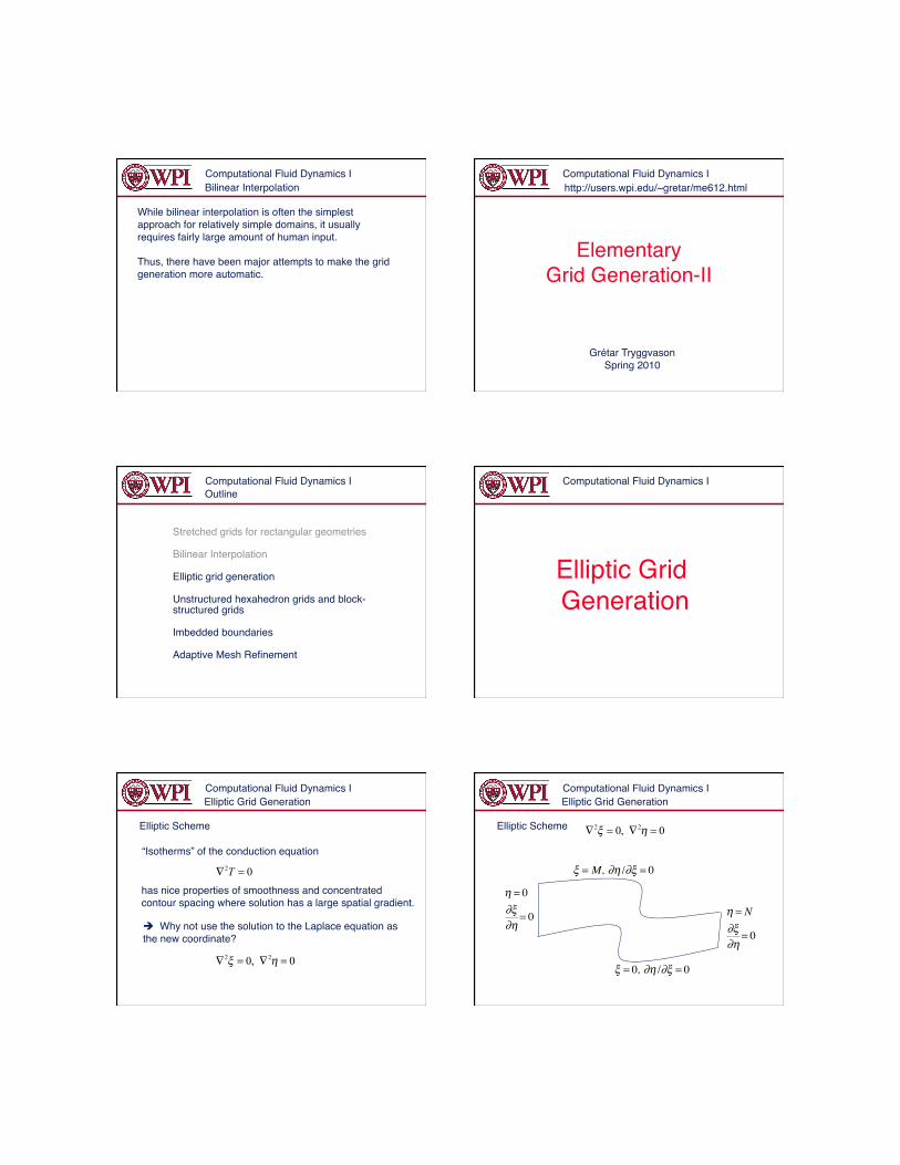
While bilinear interpolation is often the simplest approach for relatively simple domains, it usually requires fairly large amount of human input.!

Thus, there have been major attempts to make the grid generation more automatic. !


Elementary!Grid Generation-II!

http://users.wpi.edu/~gretar/me612.html!



Stretched grids for rectangular geometries!


Elliptic grid generation!

Unstructured hexahedron grids and block-structured grids!



Outline!Computational Fluid Dynamics I

Elliptic Grid Generation!


Elliptic Scheme!

“Isotherms” of the conduction equation!

02 =∇ Thas nice properties of smoothness and concentrated !contour spacing where solution has a large spatial gradient.!

Why not use the solution to the Laplace equation as the new coordinate?!

0,0 22 =∇=∇ ηξ

Elliptic Grid Generation!Computational Fluid Dynamics I Elliptic Grid Generation!

Elliptic Scheme! 0,0 22 =∇=∇ ηξ

�

ξ = 0, ∂η /∂ξ = 0

�

ξ = M, ∂η /∂ξ = 0

�

η = 0∂ξ∂η

= 0

�

η = N∂ξ∂η

= 0


Few points in regions of interest!

Need more control over the point location!

0,0 22 =∇=∇ ηξ

Elliptic Grid Generation!Computational Fluid Dynamics I

Further control can be applied by adding a source term:!

Proper choice of provides the shape of the mesh.!

In practice, instead of solving for in terms of!

, we want to solve for in terms of .!

),(),,( 22 ηξηηξξ QP =∇=∇

QP,

ηξ ,yx, yx, ηξ ,

Transform the Poisson equation into space.!( )ηξ ,



Adding the two equations:!

we obtain !�

xξ ∇2ξ + xη∇

2η = xξ P(ξ ,η) + xηQ(ξ ,η)

yξ ∇2ξ + yη∇

2η = yξ P(ξ ,η) + yηQ(ξ ,η)

( )ηξηηξηξξ QxPxJxqxqxq +−=+− 2123 2

( )ηξηηξηξξ QyPyJyqyqyq +−=+− 2123 2

where !

223

2

221

ξξ

ηξηξ

ηη

yxq

yyxxqyxq

+=

+=

+=


In discretized form (x-equation):!

�

α xi+1, j − 2xi, j + xi−1, j( ) − 0.5β xi+1, j+1 − xi+1, j−1 − xi−1, j+1 + xi−1, j−1( )

where !

�

γ xi, j+1 − 2xi, j + xi, j−1( ) + 0.5δ P xi+1, j − xi−1, j( ) + Q xi, j+1 − xi, j−1( )[ ] = 0

�

α = 0.25 xi, j+1 − xi, j−1( )2 + yi, j+1 − yi, j−1( )2[ ]

�

β = 0.25 xi+1, j − xi−1, j( ) xi, j+1 − xi, j−1( ) + yi+1, j − yi−1, j( ) yi, j+1 − yi, j−1( )[ ]

�

γ = 0.25 xi+1, j − xi−1, j( )2 + yi+1, j − yi−1, j( )2[ ]

�

δ = 116

xi+1, j − xi−1, j( ) yi, j+1 − yi, j−1( ) − yi+1, j − yi−1, j( ) xi, j+1 − xi, j−1( )[ ]2



suggested by Thompson (1977)!

�

P ξ,η( ) = − al sgn ξ −ξ l( )exp −cl ξ −ξ l( )l=1

L

∑

QP,

�

− bm sgn ξ −ξm( )exp −dm ξ −ξm( )2 + η −ηm( )2[ ]1/ 2⎛ ⎝ ⎜

⎞ ⎠ ⎟

m=1

M

∑

�

Q ξ,η( ) = − al sgn η −ηl( )exp −cl η −ηl( )l=1

L

∑

�

− bm sgn η −ηm( )exp −dm ξ −ξm( )2 + η −ηm( )2[ ]1/ 2⎛ ⎝ ⎜

⎞ ⎠ ⎟

m=1

M

∑where are chosen to generate appropriate !grid clustering.!

mlml dcba ,,,

( )⎪⎩

⎪⎨⎧

<−=>

=0if10if00if1

sgnxxx

x


Selection of!

�

P ξ,η( ) = −al sgn ξ −ξ l( )exp −cl ξ −ξ l( )QP,

Attracts grid lines to the line ξ = ξl.!al determines how strongly and !cl determines the “reach” of the attraction!

�

ξ l



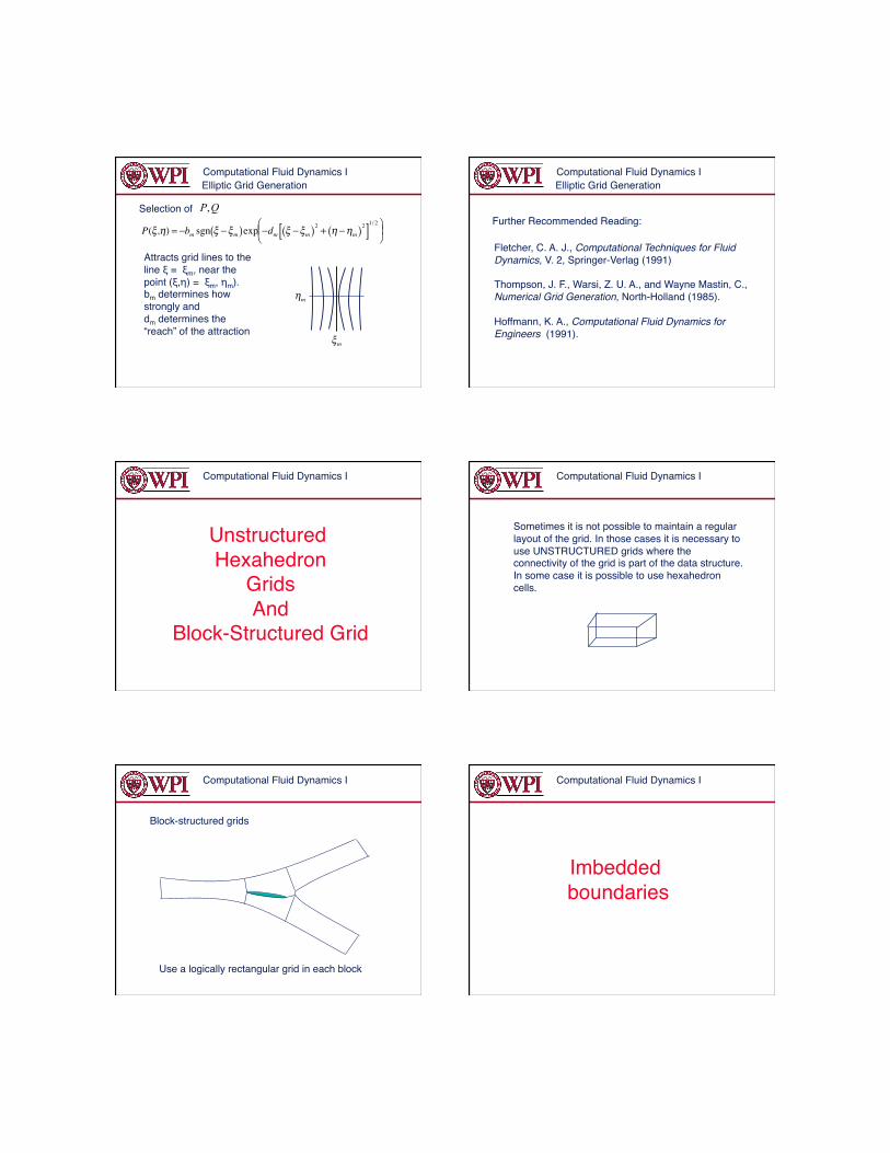
Selection of! QP,

�

P(ξ,η) = −bm sgn ξ −ξm( )exp −dm ξ −ξm( )2 + η −ηm( )2[ ]1/ 2⎛ ⎝ ⎜

⎞ ⎠ ⎟

Attracts grid lines to the line ξ = ξm, near the point (ξ,η) = ξm, ηm).!bm determines how strongly and !dm determines the “reach” of the attraction!

�

ξm�

ηm


Further Recommended Reading:!

Fletcher, C. A. J., Computational Techniques for Fluid!Dynamics, V. 2, Springer-Verlag (1991)!

Thompson, J. F., Warsi, Z. U. A., and Wayne Mastin, C., !Numerical Grid Generation, North-Holland (1985).!

Hoffmann, K. A., Computational Fluid Dynamics for !Engineers (1991).!



Unstructured Hexahedron!

Grids!And!

Block-Structured Grid!


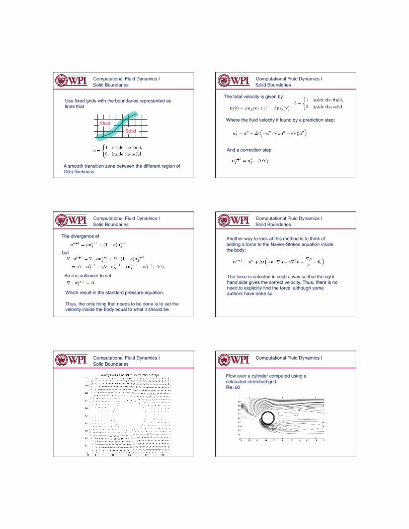
Sometimes it is not possible to maintain a regular layout of the grid. In those cases it is necessary to use UNSTRUCTURED grids where the connectivity of the grid is part of the data structure. In some case it is possible to use hexahedron cells.!


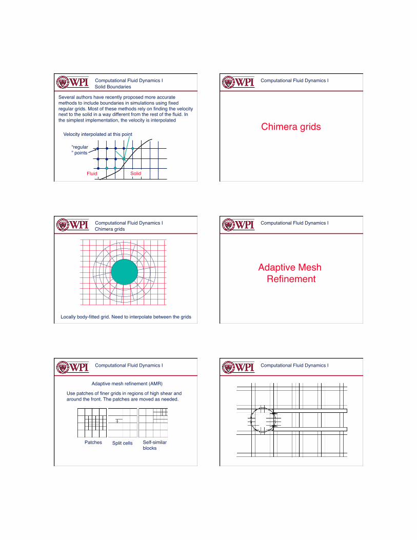
Block-structured grids!

Use a logically rectangular grid in each block!




Use fixed grids with the boundaries represented as lines that !

A smooth transition zone between the different region of O(h) thickness!

Solid Boundaries!

Solid!Fluid!

Computational Fluid Dynamics I Solid Boundaries!

The total velocity is given by!

Where the fluid velocity if found by a prediction step:!

And a correction step!


The divergence of !

but!

So it is sufficient to set!

Which result in the standard pressure equation.!

Thus, the only thing that needs to be done is to set the velocity inside the body equal to what it should be!


Another way to look at this method is to think of adding a force to the Navier-Stokes equation inside the body:!

The force is selected in such a way so that the right hand side gives the correct velocity. Thus, there is no need to explicitly find the force, although some authors have done so.!



Flow over a cylinder computed using a colocated stretched grid!Re=60!


Several authors have recently proposed more accurate methods to include boundaries in simulations using fixed regular grids. Most of these methods rely on finding the velocity next to the solid in a way different from the rest of the fluid. In the simplest implementation, the velocity is interpolated!

Solid Boundaries!

Solid!Fluid!

Velocity interpolated at this point!

“regular” points!


Chimera grids!

Computational Fluid Dynamics I Chimera grids!

Locally body-fitted grid. Need to interpolate between the grids!




Adaptive mesh refinement (AMR)!

Use patches of finer grids in regions of high shear and around the front. The patches are moved as needed.!

Split cells! Self-similar blocks!

Patches!


Computational Fluid Dynamics I Computational Fluid Dynamics I

Computational Fluid Dynamics I Computational Fluid Dynamics I

From Agreasar et al.!


Grid generation for complex geometries is usually a major task, requiring both large amount of time and money. Structured grids generally lead to fast and accurate flow solvers and are therefore preferred where the cost of generating the grid is not excessive.!

For situations where the complexity of the domain is such that grid generation is very expensive and where the user can live with modest accuracy, unstructured grids are generally used.!


Unstructured!Grids!

http://users.wpi.edu/~gretar/me612.html!



Unstructured versus structured grids!

structured grids: an ordered layout of grid points.!

unstructured grids: an arbitrary layout of grid points. Information about the layout must be provided!

Unstructured grids!Computational Fluid Dynamics I

Since the points are laid out in an irregular unstructured way, the point location and connectivity must be stored!

Unstructured grids can consist of arbitrarily shaped control volumes but tetrahedrons (pyramids) and hexahedrons (boxes) are most common!

Unstructured grids!


For a cell based scheme each cell is a control volume and we solve for the average values in each cell!

Cell!

Edge!

Face!


For vertex based schemes a control volume is constructed by dividing up the cells next to the vertex!

Cell!

Edge!

Face!The cells can be divided by drawing a line perpendicular to each edge. The corners of the control volume are where two such lines intersect!

Unstructured grids!


Data Structure:!Indirect addressing!

x1! y1!

x2! y2!x3! y3!x4! y4!x5! y5!.! .!

Node coordinates!

n11! n12! n13!

n21! n22! n23!

n31! n32! n33!

n41! n42! n43!

n51! n52! n53!

.! .! .!

Element corners!

x-coordinate of the first corner point of element m: x(m(1))!

Usually it also helps if the elements know about their neighbors!

n11!

n12!

n13!Elem 1!


The finite volume method is usually used to derive numerical approximations for unstructured grids. However, finite element methods and “mesh free” methods also use unstructured grids!

Here we will briefly outline a vertex centered method for the advection/diffusion equation!

Unstructured grids!


Vertex centered advection diffusion equation!

�

∂f∂t

+ ∇ ⋅uf = ν∇2 f

Integrate over a control volume!

�

∂f∂tdv +

V∫ ∇ ⋅uf dvV∫ = ν ∇2 f dv

V∫

�

∂∂t

fdv +V∫ fu ⋅nds

S∫ = ν ∇f ⋅ndsS∫

Convert volume integrals to surface integrals!


�

A jddt

f j = − feall edges∑ ue ⋅neΔse + ν Δfe

all edges∑ Δse

le

�

fe = 12

f j + f i( )Δfe = f j − f i

ue = 12u j + u i( )

Node i!Node j!Aj!

le!Δse!

�

f j = fdvV j∫

ne =x j − xi

x j − xi

le = x j − xi

Numerical approximation!

Generally we loop over the elements!

Unstructured grids!


Generation of unstructured triangular grids:!Advancing front: Start at one boundary and keep adding points until you run into another boundary!

Delauny triangulation: generate a coarse grid and refine!


Originally, triangular grid were developed for the compressible Euler equations. Approximating the viscous fluxes and enforcing incompressibility is more complex. For boundary layer like flow, sometimes hybrid tetrahedron/hexahedron grids have been advocated!

More resources:!http://www.erc.msstate.edu http://www.cfd-online.com/ http://capella.colorado.edu/~laney/thompson.htm

Unstructured grids!

Stretched Grids for Rectangular Domainsgtryggva/CFD-Course2010/2010-Lecture-17.pdfStretched grids...

Documents

Transcript of Stretched Grids for Rectangular Domainsgtryggva/CFD-Course2010/2010-Lecture-17.pdfStretched grids...