Stretched Grids - University of Notre Damegtryggva/CFD-Course/2011-Lecture-25.pdf · 2011-03-22 ·...
8
Computational Fluid Dynamics Elementary Grid Generation Grétar Tryggvason Spring 2011 http://www.nd.edu/~gtryggva/CFD-Course/ Computational Fluid Dynamics Stretched grids for rectangular geometries Bilinear Interpolation Elliptic grid generation Unstructured hexahedron grids and block- structured grids Imbedded boundaries Adaptive Mesh Refinement Outline Computational Fluid Dynamics There are two main reasons for using grids that are not rectangular with uniform grid spacing 1. Representing a domain with complex boundaries 2. Put grid points in parts of the domain where high resolution is needed Frequently, it is necessary to deal with both issues Computational Fluid Dynamics Stretched Grids Computational Fluid Dynamics Fine grid needed here! Gridlines are straight but unevenly spaced: Computational Fluid Dynamics Simple stretching ! x x ! Boundary layer Internal layer x = x ! ()
Transcript of Stretched Grids - University of Notre Damegtryggva/CFD-Course/2011-Lecture-25.pdf · 2011-03-22 ·...
Computational Fluid Dynamics
Elementary!Grid Generation!
Grétar Tryggvason !Spring 2011!
http://www.nd.edu/~gtryggva/CFD-Course/!Computational Fluid Dynamics
Stretched grids for rectangular geometries!!
Bilinear Interpolation!!
Elliptic grid generation!!
Unstructured hexahedron grids and block-structured grids!
!Imbedded boundaries!
!Adaptive Mesh Refinement!
Outline!
Computational Fluid Dynamics
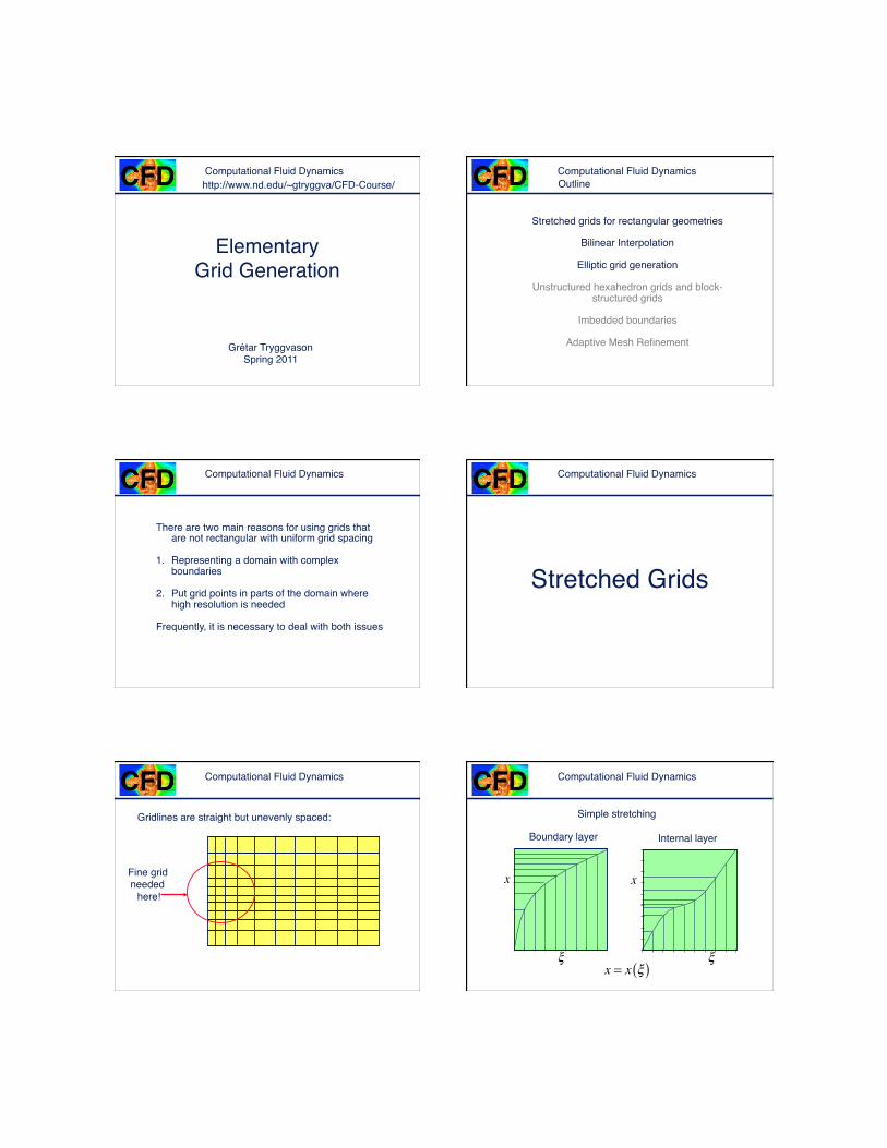
There are two main reasons for using grids that are not rectangular with uniform grid spacing!
!1. Representing a domain with complex
boundaries!
2. Put grid points in parts of the domain where high resolution is needed!
Frequently, it is necessary to deal with both issues!
Computational Fluid Dynamics
Stretched Grids!
Computational Fluid Dynamics
Fine grid needed
here!!
Gridlines are straight but unevenly spaced:!
Computational Fluid Dynamics
Simple stretching!
!
x
x
!
Boundary layer! Internal layer!
x = x !( )

Computational Fluid Dynamics
Stretching functions-examples!
“one-sided” boundary layer!
0 0.2 0.4 0.6 0.8 10
0.5
1
1.5
2
x
0 0.2 0.4 0.6 0.8 10
0.5
1
1.5
2
x
x = !n
x = !2
x = !
Computational Fluid Dynamics Stretching functions-examples!
Internal layer!
x = L! + A xC " L!( ) 1" !( )!Line!
Zero at endpoints!Changes signs at xc!
“strength” and gives concentrates points inside domain (A>0) or at the
ends (A<0)!
Computational Fluid Dynamics Stretching functions-examples!
0 0.2 0.4 0.6 0.8 10
0.5
1
1.5
2
x
A=2.5 x=1 % A program to test 1D grid refinement.!!L=2.0;xc=1.0; A=2.5!s=[0:0.05:1];n=size(s);!!for i=1:n(2), ! x(i)=L*s(i)+A*(xc-L*s(i))*s(i)*(1-s(i));!End!plot(s,x,'LineWidth',2);hold on!!for i=1:n(2),! plot([s(i),s(i)],[0.0, x(i)]);! plot([0.0,s(i)],[x(i), x(i)]);!end!xlabel('\xi','Fontsize',18)!ylabel('x','Fontsize',18)!set(gca,'Box','on'); !set(gca,'Fontsize',18, 'LineWidth',2)!plot([0,1],[0,L],'r')!text(0.05,L-0.1,['A=',num2str(A),...!' x=',num2str(xc)],'Fontsize',18)!!hold off; % print -depsc exampleplot!0 0.2 0.4 0.6 0.8 1
0
0.5
1
1.5
2
x
A= 1.5; x=1
x = x !( )
x = x !( )
Computational Fluid Dynamics
The MAC method on Stretched
Grids!
Computational Fluid Dynamics Computational Fluid Dynamics Stretched grids!
Special case:!
x = x !( )y = y "( )
q1 = y!2
q2 = 0q3 = x"
2
J = x! y"
u = 1JUx!( ) = 1
x! y"Ux!( ) = U
y"
v = 1JVy!( ) = 1
y! x"Vy!( ) = V
x"
y!"u"#
+ x#"v"!
= 0
1x!
"u"!
+ 1y#
"v"#
= 00=!!+
!!
"#VU

Computational Fluid Dynamics
Approximate the conservation equation!
x! = xi+1 " xi1
= #xi+1/ 2
y! =y j+1 " y j
1= #y j+1/ 2
ui+1/ 2, j ! ui!1/ 2, j"xi
+vi, j+1/ 2 ! vi, j!1/ 2
"y j
= 0
!" = !# =1
1x!
"u"!
+ 1y#
"v"#
= 0
!y j = 12!y j+1/ 2 + !y j"1/ 2( )
Define:!
!xi = 12
!xi+1/ 2 + !xi"1/ 2( )
Stretched grids!Computational Fluid Dynamics
!u!t
+1x"
!u2
!"+
1y#
!vu!#
= $1x"
!p!"
+ % 1x"
!!"
u"
x"
&
'(
)
*+ +
1y#
!!#
u#
y#
&
'(
)
*+
,
-..
/
011
u-Momentum Equation!
ui+1/ 2, jn+1 ! ui+1/ 2, j
n
"t= !
(u2 )i+1, jn ! (u2 )i, j
n
"xi+1/ 2
!(uv)
i+1/ 2, j+1/ 2
n ! (uv)i+1/ 2, j!1/ 2
n
"y j
!Pi+1, j ! Pi, j
"xi+1/ 2
+ # 1"xi+1/ 2
ui+3/ 2, j
n! u
i+1/ 2, j
n
"xi+1
!u
i+1/ 2, j
n! u
i!1/ 2, j
n
"xi
$
%&&
'
())
$
%
&&
+1"y j
ui+1/ 2, j+1
n! u
i+1/ 2, j
n
"y j+1/ 2
!u
i+1/ 2, j
n! u
i+1/ 2, j!1
n
"y j!1/ 2
$
%&&
'
())
'
(
))
Stretched grids!
Computational Fluid Dynamics
!v!t
+1x"
!uv!"
+1y#
!v2
!#= $
1y#
!p!#
+ % 1x"
!!"
v"
x"
&
'(
)
*+ +
1y#
!!#
v#y#
&
'(
)
*+
,
-..
/
011
v-Momentum Equation!
vi, j+1/ 2n+1 ! vi, j+1/ 2
n
"t= !
(uv)i+1, j+1/ 2n ! (uv)i, j+1/ 2
n
"xi+1/ 2
!(v2 )
i, j+1
n ! (v2 )i, j
n
"y j
!Pi, j+1 ! Pi, j
"y j+1/ 2
+ # 1"xi
vi+1, j+1/ 2
n! v
i, j+1/ 2
n
"xi+1/ 2
!v
i, j+1/ 2
n! v
i!1, j+1/ 2
n
"xi!1/ 2
$
%&&
'
())
$
%
&&
+1
"y j+1/ 2
vi, j+3/ 2
n! v
i, j+1/ 2
n
"y j+1
!v
i, j+1/ 2
n! v
i, j!1/ 2
n
"y j
$
%&&
'
())
'
(
))
Stretched grids!Computational Fluid Dynamics
The pressure equation is:!
1!xi
Pi+1, j " Pi, j
!xi+1/ 2
"Pi, j " Pi"1, j
!xi"1/ 2
#
$%
&
'( +
1!y j
Pi, j+1 " Pi, j
!y j+1/ 2
"Pi, j " Pi, j"1
!y j"1/ 2
#
$%
&
'(
= !tu
i+1/ 2, j
*" u
i"1/ 2, j
*
!xi
"v
i, j+1/ 2
*" v
i, j"1/ 2
*
!y j
#
$%%
&
'((
Which can be solved by iteration!
Stretched grids!
Computational Fluid Dynamics
Colocated stretched grids!
Re=10!
Stretched grids!Computational Fluid Dynamics
For one dimensional stretched grids, we simply replace the global Δx by the local Δx!
pi,j! ui+1/2,j!
Δxi+1/2!
Δxi!
ui-1/2,j! pi+1,j!
Stretched grids!

Computational Fluid Dynamics
Bilinear Interpolation!
Computational Fluid Dynamics
Simples grid generation is to break the domain into blocks and use bilinear interpolation within each block!
As an example,
we will write a simple
code to grid the domain to the right!
(x1,y1)!
(x2,y2)!(x3,y3)!
(x4,y4)!(x5,y5)!
(x6,y6)!(x7,y7)!
(x8,y8)!
Bilinear Interpolation!
Computational Fluid Dynamics
Start by breaking the domain into blocks!
Then grid each block separately!
(x1,y1)!
(x2,y2)!(x3,y3)!
(x4,y4)!(x5,y5)!
(x6,y6)!(x7,y7)!
(x8,y8)!
Bilinear Interpolation!Computational Fluid Dynamics
P1,0!1!
2!
3!
P1,3!
P1,2=P2,3!
P1,1=P2,0! P2,1=P3,0!
P3,2! P3,1!P2,2=P3,3!
Start by breaking the domain into blocks!
Then grid each block separately!
Bilinear Interpolation!
Computational Fluid Dynamics
2!
P1,0!1!
P1,3!
P1,2!
P1,1!
3!
P3,0!
P3,2! P3,1!
P2,2!
P3,3!
P2,1!P2,0!
P2,3!
Start by breaking the domain into blocks!
Then grid each block separately!
Bilinear Interpolation!Computational Fluid Dynamics
Consider an arbitrary shaped quadrilateral block!1. Select the ξ and ξ direction.!
(x0,y0)!
(x1,y1)!
(x2,y2)!(x3,y3)!
!
!
N!
M!2. Divide the
opposite sides evenly with N points in the ξ direction and !
M in the ξ direction and draw
straights line between the points
on the opposite sides!
Bilinear Interpolation!
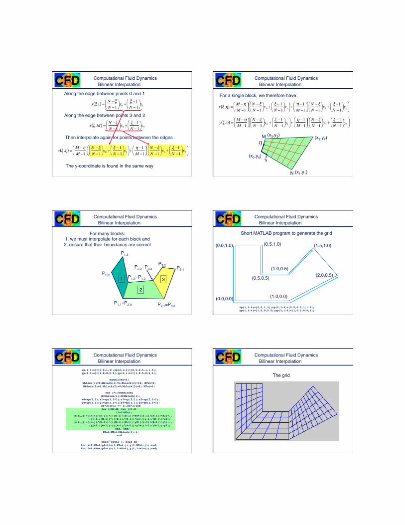
Computational Fluid Dynamics
x ! ,1( ) =N "!N "1
# $
% & x0 +
! "1N "1
# $
% & x1
Along the edge between points 0 and 1!
Along the edge between points 3 and 2!
x ! ,M( ) =N "!N "1
# $
% & x3 +
! "1N "1
# $
% & x2
Then interpolate again for points between the edges!
x ! ,"( ) =M #"M #1
$ %
& ' N #!N #1
$ %
& ' x0 +
! #1N #1
$ %
& ' x1
$ % ( &
' +
"#1M #1
$ %
& '
N #!N #1
$ %
& ' x3 +
! #1N #1
$ %
& ' x2
$ % ( &
'
The y-coordinate is found in the same way!
Bilinear Interpolation!Computational Fluid Dynamics
x ! ,"( ) =M #"M #1
$ %
& ' N #!N #1
$ %
& ' x0 +
! #1N #1
$ %
& ' x1
$ % ( &
' +
"#1M #1
$ %
& '
N #!N #1
$ %
& ' x3 +
! #1N #1$ %
& ' x2
$ % ( &
'
y ! ,"( ) =M #"M #1
$ %
& ' N #!N #1
$ %
& ' y0 +
! #1N #1
$ %
& ' y1
$ % ( &
' +
"#1M #1
$ %
& '
N #!N #1
$ %
& ' y3 +
! #1N #1$ %
& ' y2
$ % ( &
'
(x0,y0)!
(x1,y1)!
(x2,y2)!(x3,y3)!
!
!
N!
M!
For a single block, we therefore have:!
Bilinear Interpolation!
Computational Fluid Dynamics
For many blocks:!1. we must interpolate for each block and !2. ensure that their boundaries are correct!
P1,0!1!
2!
3!
P1,3!
P1,2=P1,2!
P1,1=P2,0! P2,1=P3,0!
P3,2! P3,1!P2,2=P3,3!
Bilinear Interpolation!Computational Fluid Dynamics
Short MATLAB program to generate the grid!
xp(1,1:4)=[0,0,1,2];xp(2,1:4)=[0.5,0.5,1,1.5];!yp(1,1:4)=[1,0,0,0.5];yp(2,1:4)=[1,0.5,0.5,1];!
(0.0,1.0)!
(0.0,0.0)!
(0.5,1.0)!
(1.0,0.5)!
(1.0,0.0)!
(2.0,0.5)!(0.5,0.5)!
(1.5,1.0)!
Bilinear Interpolation!
Computational Fluid Dynamics
xp(1,1:4)=[0,0,1,2];xp(2,1:4)=[0.5,0.5,1,1.5];!yp(1,1:4)=[1,0,0,0.5];yp(2,1:4)=[1,0.5,0.5,1];!
!NumBlocks=3;!
Nblock(1)=8;Nblock(2)=5;Nblock(3)=12; NTot=0;!Mblock(1)=6;Mblock(2)=6;Mblock(3)=6; MTot=6;!
!for l=1:NumBlocks!
N=Nblock(l);M=Mblock(l);! x0=xp(1,l);x1=xp(1,l+1);x3=xp(2,l);x2=xp(2,l+1);! y0=yp(1,l);y1=yp(1,l+1);y3=yp(2,l);y2=yp(2,l+1);!
Nf=2;if(l == 1),Nf=1;end! for i=Nf:N, for j=1:M !!
ii=i+NTot;! x(ii,j)=((M-j)/(M-1))*(((N-i)/(N-1))*x0+((i-1)/(N-1))*x1)+...!
((j-1)/(M-1))*(((N-i)/(N-1))*x3+((i-1)/(N-1))*x2);! y(ii,j)=((M-j)/(M-1))*(((N-i)/(N-1))*y0+((i-1)/(N-1))*y1)+...!
((j-1)/(M-1))*(((N-i)/(N-1))*y3+((i-1)/(N-1))*y2);! end, end;!
NTot=NTot+Nblock(l)-1;!end!!
axis(’equal'), hold on!for j=1:MTot;plot(x(1:NTot,j),y(1:NTot,j));end;!for i=1:NTot;plot(x(i,1:MTot),y(i,1:MTot));end;!
Bilinear Interpolation!Computational Fluid Dynamics
The grid!
Bilinear Interpolation!

Computational Fluid Dynamics
Sometimes the grid can be improved by smoothing. The simples smoothing is to
replace the coordinate of each grid point by the average of the coordinates around it. This
process can be repeated several times to improve the smoothness.!
Bilinear Interpolation!
x i, j( ) = 0.25* x i +1, j( ) + x i !1, j( ) + x i, j +1( ) + x i, j !1( )( )y i, j( ) = 0.25* y i +1, j( ) + y i !1, j( ) + y i, j +1( ) + y i, j !1( )( )
Computational Fluid Dynamics
The grid after two smoothing iterations!
Bilinear Interpolation!
Computational Fluid Dynamics
Bilinear Interpolation can also be used for curved boundaries, if the points on the
boundaries are given.!
Higher order Interpolation functions can also be used to generate stretched grids for
complex boundaries.!
Bilinear Interpolation!Computational Fluid Dynamics
The grid generation results in an array of x and y coordinates for each grid point:!
!For simple problems we can include the grid generator in the fluid solver and generate the coordinates before
we solve for the fluid motion!!
For more complex problems the grid generation step is usually separated from the flow solver and the grid
points are read from a file!!
For commercial codes you can generally use many different grid generators—as long as the data format is
consistent !
Bilinear Interpolation!
x !,"( ), " !,"( )
Computational Fluid Dynamics Bilinear Interpolation!
Flow in an elbow, computed using a body fitted grid, using the streamfunction-vorticity formulation of the Navier-
Stokes equations!
Grid—bilinear interpolation with smoothing!
Streamfunction!
Computational Fluid Dynamics Bilinear Interpolation!
While bilinear interpolation is often the simplest approach for relatively simple domains, it usually
requires fairly large amount of human input.!!
Thus, there have been major attempts to make the grid generation more automatic. !
Computational Fluid Dynamics
Elliptic Grid Generation!
Computational Fluid Dynamics
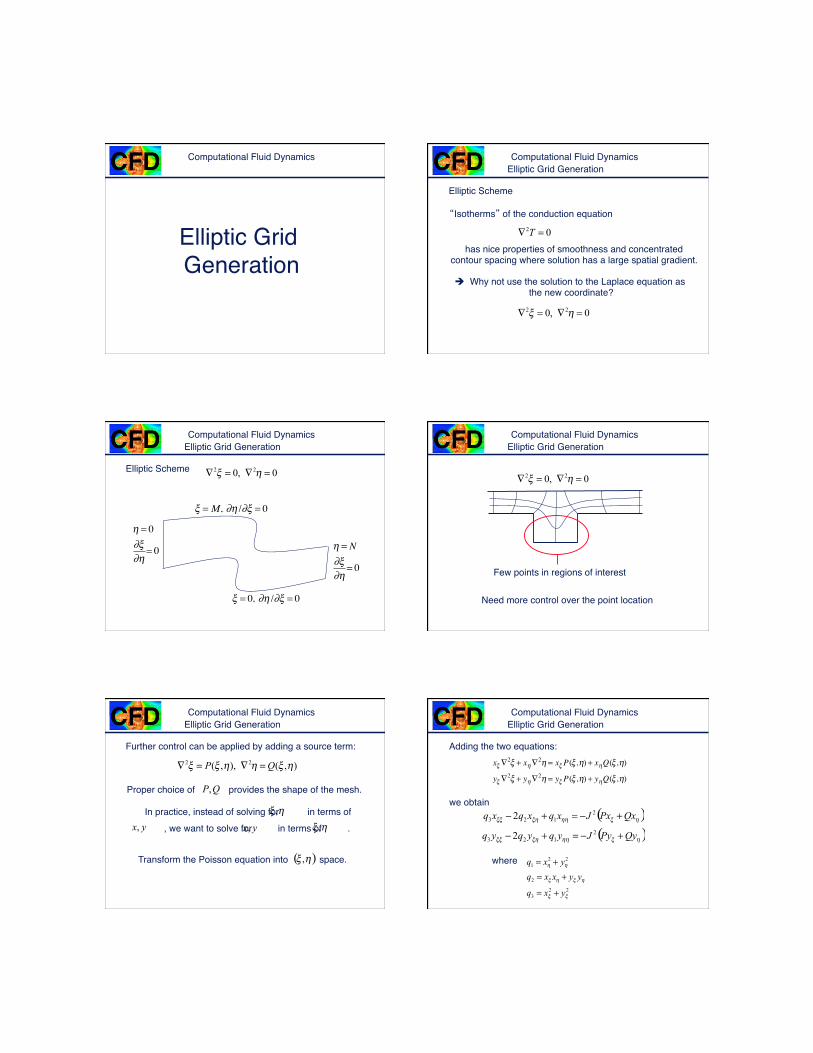
Elliptic Scheme!
“Isotherms” of the conduction equation!
02 =! Thas nice properties of smoothness and concentrated !
contour spacing where solution has a large spatial gradient.!
Why not use the solution to the Laplace equation as the new coordinate?!
0,0 22 =!=! "#
Elliptic Grid Generation!
Computational Fluid Dynamics Elliptic Grid Generation!
Elliptic Scheme! 0,0 22 =!=! "#
! = 0, "# /"! = 0
! = M, "# /"! = 0
! = 0"#"!
= 0
! = N"#"!
= 0
Computational Fluid Dynamics
Few points in regions of interest!
Need more control over the point location!
0,0 22 =!=! "#
Elliptic Grid Generation!
Computational Fluid Dynamics
Further control can be applied by adding a source term:!
Proper choice of provides the shape of the mesh.!
In practice, instead of solving for in terms of! , we want to solve for in terms of .!
),(),,( 22 !"!!"" QP =#=#
QP,
!" ,yx, yx, !" ,
Transform the Poisson equation into space.!( )!" ,
Elliptic Grid Generation!Computational Fluid Dynamics
Adding the two equations:!
we obtain !
x! "2! + x#"
2# = x! P(! ,#) + x#Q(! ,#)
y! "2! + y#"
2# = y! P(! ,#) + y#Q(! ,#)
( )!"!!"!"" QxPxJxqxqxq +#=+# 2123 2
( )!"!!"!"" QyPyJyqyqyq +#=+# 2123 2
where !
223
2
221
!!
"!"!
""
yxq
yyxxq
yxq
+=
+=
+=
Elliptic Grid Generation!
Computational Fluid Dynamics
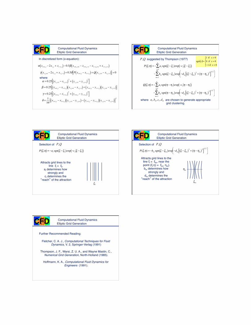
In discretized form (x-equation):!
! xi+1, j " 2xi, j + xi"1, j( ) " 0.5# xi+1, j+1 " xi+1, j"1 " xi"1, j+1 + xi"1, j"1( )
where !
! xi, j+1 " 2xi, j + xi, j"1( ) + 0.5# P xi+1, j " xi"1, j( ) + Q xi, j+1 " xi, j"1( )[ ] = 0
! = 0.25 xi, j+1 " xi, j"1( )2 + yi, j+1 " yi, j"1( )2[ ]
! = 0.25 xi+1, j " xi"1, j( ) xi, j+1 " xi, j"1( ) + yi+1, j " yi"1, j( ) yi, j+1 " yi, j"1( )[ ]
! = 0.25 xi+1, j " xi"1, j( )2 + yi+1, j " yi"1, j( )2[ ]
! = 116
xi+1, j " xi"1, j( ) yi, j+1 " yi, j"1( ) " yi+1, j " yi"1, j( ) xi, j+1 " xi, j"1( )[ ]2
Elliptic Grid Generation!Computational Fluid Dynamics
suggested by Thompson (1977)!
P !,"( ) = # al sgn ! #! l( )exp #cl ! #! l( )l=1
L
$
QP,
! bm sgn " !"m( )exp !dm " !"m( )2 + # !#m( )2[ ]1/ 2$ % &
' ( )
m=1
M
*
Q !,"( ) = # al sgn " #"l( )exp #cl " #"l( )l=1
L
$
! bm sgn " !"m( )exp !dm # !#m( )2 + " !"m( )2[ ]1/ 2$ % &
' ( )
m=1
M
*where are chosen to generate appropriate !
grid clustering.!mlml dcba ,,,
( )!"
!#$
<%=>
=0if10if00if1
sgnxxx
x
Elliptic Grid Generation!
Computational Fluid Dynamics
Selection of!
P !,"( ) = #al sgn ! #! l( )exp #cl ! #! l( )QP,
Attracts grid lines to the line ξ = ξl.!
al determines how strongly and !
cl determines the “reach” of the attraction!
! l
Elliptic Grid Generation!Computational Fluid Dynamics
Selection of! QP,
P(!,") = #bm sgn ! #!m( )exp #dm ! #!m( )2 + " #"m( )2[ ]1/ 2$ % &
' ( )
Attracts grid lines to the line ξ = ξm, near the point (ξ,η) = ξm, ηm).!bm determines how
strongly and !dm determines the
“reach” of the attraction!
!m
!m
Elliptic Grid Generation!
Computational Fluid Dynamics
Further Recommended Reading:!
Fletcher, C. A. J., Computational Techniques for Fluid!Dynamics, V. 2, Springer-Verlag (1991)!
!Thompson, J. F., Warsi, Z. U. A., and Wayne Mastin, C., !
Numerical Grid Generation, North-Holland (1985).!!
Hoffmann, K. A., Computational Fluid Dynamics for !Engineers (1991).!
Elliptic Grid Generation!