
CONFOCAL MICROSCOPY - LINE SCANNING SETUP WITH …CONFOCAL MICROSCOPY - LINE SCANNING SETUP WITH...
103
CONFOCAL MICROSCOPY - LINE SCANNING SETUP WITH HIGH BRIGHTNESS LED A Thesis Presented by Ali Vakili to Department of Electrical and Computer Engineering in partial fulfillment of the requirements for the degree of Master of Science in Electrical Engineering Northeastern University Boston, Massachusetts April 2014
Transcript of CONFOCAL MICROSCOPY - LINE SCANNING SETUP WITH …CONFOCAL MICROSCOPY - LINE SCANNING SETUP WITH...

CONFOCAL MICROSCOPY - LINE SCANNING SETUP
WITH HIGH BRIGHTNESS LED
A Thesis Presented
by
Ali Vakili
to
Department of Electrical and Computer Engineering
in partial fulfillment of the requirements
for the degree of
Master of Science
in
Electrical Engineering
Northeastern University
Boston, Massachusetts
April 2014

NORTHEASTERN UNIVERSITY
Graduate School of Engineering
Thesis Title: Confocal Microscopy - Line Scanning Setup with High Brightness
LED.
Author: Ali Vakili.
Department: Electrical and Computer Engineering.
Approved for Thesis Requirements of the Master of Science Degree:
Thesis Supervisor: Prof. Charles DiMarzio Date
Thesis committee: Dr. Milind Rajadhyaksha Date
Thesis Committee: Prof. Mark Niedre Date
Department Chair: Prof. Sheila S. Hemami Date
Director of the Graduate School: Prof. Sara Wadia-Fascetti Date

Acknowledgments
I would like to express my special appreciation and thanks to my advisor Professor
Charles A. DiMarzio, who has been a tremendous mentor for me and gave me the
opportunity to work under his supervision in Optical Science Laboratory. I also want
to thank Dr. Milind Rajadhyaksha who co-advised me during this research. Also I
want to express my appreciation towards Professor Mark Niedre and Dr. Milind Ra-
jadhyaksha for serving on my thesis committee. I would like to thank all my friends
and colleagues in optical science laboratory for all their support and contributions.
Many thanks to Joseph Hollmann for his contribution in the projects with his great
ideas and amazing MATLAB skills and also, Ali Golabchi for providing many con-
structive feedback on this thesis. At the end, I would like to thank my family and all
my friends who always supported me.
iii

Contents
Acknowledgments iii
1 Introduction 1
1.1 Optical Imaging . . . . . . . . . . . . . . . . . . . . . . . . . . . . . . 3
1.2 Optical Sectioning . . . . . . . . . . . . . . . . . . . . . . . . . . . . 6
1.3 Confocal Microscopy . . . . . . . . . . . . . . . . . . . . . . . . . . . 8
1.3.1 Point Scanning . . . . . . . . . . . . . . . . . . . . . . . . . . 11
1.3.2 Line Scanning . . . . . . . . . . . . . . . . . . . . . . . . . . . 13
1.4 Components in Confocal Microscope . . . . . . . . . . . . . . . . . . 16
1.4.1 Pinhole or Slit . . . . . . . . . . . . . . . . . . . . . . . . . . . 16
1.4.2 Beam Splitter . . . . . . . . . . . . . . . . . . . . . . . . . . . 18
1.4.3 Detector . . . . . . . . . . . . . . . . . . . . . . . . . . . . . . 20
2 Light Sources 25
2.1 Introduction . . . . . . . . . . . . . . . . . . . . . . . . . . . . . . . . 25
2.1.1 Brightness . . . . . . . . . . . . . . . . . . . . . . . . . . . . . 25
2.1.2 Wavelength . . . . . . . . . . . . . . . . . . . . . . . . . . . . 27
2.1.3 Coherence . . . . . . . . . . . . . . . . . . . . . . . . . . . . . 28
2.2 Laser Light Sources . . . . . . . . . . . . . . . . . . . . . . . . . . . . 30
iv

2.2.1 Introduction to Laser . . . . . . . . . . . . . . . . . . . . . . . 30
2.2.2 Laser Diode . . . . . . . . . . . . . . . . . . . . . . . . . . . . 35
2.3 Non-Laser Light Sources . . . . . . . . . . . . . . . . . . . . . . . . . 36
2.3.1 Arc Lamps . . . . . . . . . . . . . . . . . . . . . . . . . . . . . 36
2.3.2 Light Emitting Diode . . . . . . . . . . . . . . . . . . . . . . . 37
2.3.3 High Brightness LED . . . . . . . . . . . . . . . . . . . . . . . 39
2.4 Summary . . . . . . . . . . . . . . . . . . . . . . . . . . . . . . . . . 39
3 Scattering Medium and Pupil Configurations 40
3.1 Scattering Media and Gating Mechanism . . . . . . . . . . . . . . . . 40
3.2 Pupil Configurations . . . . . . . . . . . . . . . . . . . . . . . . . . . 44
3.2.1 Full Pupil Configuration . . . . . . . . . . . . . . . . . . . . . 44
3.2.2 Half Pupil Configuration . . . . . . . . . . . . . . . . . . . . . 46
3.2.3 Divided Pupil Configuration . . . . . . . . . . . . . . . . . . . 46
3.2.4 Comparison . . . . . . . . . . . . . . . . . . . . . . . . . . . . 48
4 Experiments and Results 50
4.1 Dual Wedge Confocal Microscope . . . . . . . . . . . . . . . . . . . . 51
4.1.1 Dual Wedge Scanner . . . . . . . . . . . . . . . . . . . . . . . 51
4.1.2 Fluorescence Modes . . . . . . . . . . . . . . . . . . . . . . . . 54
4.1.3 Results . . . . . . . . . . . . . . . . . . . . . . . . . . . . . . . 58
4.1.4 Conclusion . . . . . . . . . . . . . . . . . . . . . . . . . . . . . 61
4.2 Line Scanning Confocal Microscope . . . . . . . . . . . . . . . . . . . 61
4.2.1 Instrumentation . . . . . . . . . . . . . . . . . . . . . . . . . . 62
4.2.2 Resolution Measurement . . . . . . . . . . . . . . . . . . . . . 64
4.2.3 Results . . . . . . . . . . . . . . . . . . . . . . . . . . . . . . . 67
v

4.3 High Brightness LED as Light Source . . . . . . . . . . . . . . . . . . 68
4.3.1 LED Specifications . . . . . . . . . . . . . . . . . . . . . . . . 69
4.3.2 Design . . . . . . . . . . . . . . . . . . . . . . . . . . . . . . . 71
4.3.3 Results . . . . . . . . . . . . . . . . . . . . . . . . . . . . . . . 72
5 Conclusion 76
6 Future Work 79
6.1 Quantify Multiply Scattered Photons Rejection . . . . . . . . . . . . 79
6.2 Image Larger Area with Dual-Line Scanning . . . . . . . . . . . . . . 80
6.3 Laser-Driven Light Sources . . . . . . . . . . . . . . . . . . . . . . . . 82
Bibliography 83
vi

List of Figures
1.1 Concept of numerical aperture. a) specimen is illuminated by a collimated beam,
then numerical aperture is defined as, NA = nsin(α). b) A condenser has a
numerical aperture the same as that of the objective lens. In this case, working
aperture is the sum of numerical aperture of objective lens and condenser, therefore
NA = nsin(2α). Figure taken from ZEISS microscopy online campus . . . . . . 4
1.2 Point spread function and Airy disk definition. a) Airy disk pattern generated form
light diffracted in specimen. b) 3D representations of the diffraction pattern on the
image plane, known as the point-spread function. c) An Airy disk is the region
enclosed by the first minimum of the Airy pattern and contains approximately
84% of the energy. Figure taken from ZEISS microscopy online campus . . . . . 5
1.3 Two Airy disks close to each other. dmin is the minimum distance that each of
the two Airy disks can be resolved by the human eye. Figure taken from ZEISS
microscopy online campus . . . . . . . . . . . . . . . . . . . . . . . . . . 6
1.4 Rayleigh criterion, two Airy disks are considered resolvable if the valley between the
peaks is about 20%-30% of the maximum. Figure taken from Nikon Instruments,
Inc. website . . . . . . . . . . . . . . . . . . . . . . . . . . . . . . . . . 7
vii

1.5 Illumination method comparison between conventional and confocal microscopes.
In wide-field illumination, a large volume of the specimen is illuminated. However
in confocal microscopy, a very small volume of the specimen is exposed [1]. . . . 9
1.6 Comparison of wide-field(upper row) and confocal microscopy(lower row). (a) and
(b) mouse brain hippocampus thick section. (c) and (d) Thick section of rat smooth
muscle. (e) and (f) Sunflower pollen grain [1] . . . . . . . . . . . . . . . . . 10
1.7 Typical confocal microscope. Excitation light is directed to the sample by a dichroic
mirror or beam splitter. Two galvanometer mirror scan the beam on the sample in
two direction and objective lens, focuses the beam onto a diffraction limited spot
on specimen. Light coming back from the specimen, travels the same path to the
dichroic mirror which transmit the beam to the confocal pinhole and the detector.
A/D which is synchronized with scanner is then used to collect information and
store in the computer. Image is then reconstructed in computer and is displayed
on the monitor [1]. . . . . . . . . . . . . . . . . . . . . . . . . . . . . . . 12
1.8 Rotating polygon mirror used as scanner. A motor rotates the mirror and contin-
uously scans the beam on the specimen. Unlike galvo scanner, it is not needed to
return the mirror to the initial position. Therefore it is easier to synchronize the
scanner with data acquisition board. Backscattered light returns the same path to
the polygon mirror. Figure taken from LEYBOLD Photonics educational kit website 13
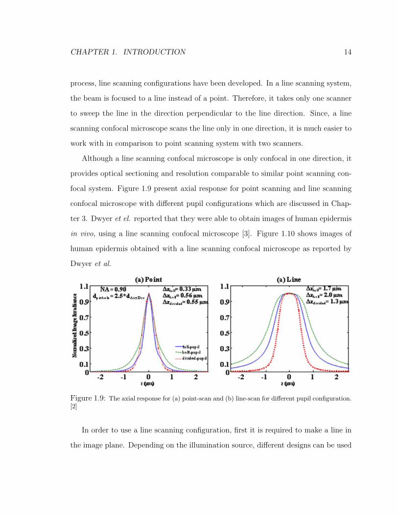
1.9 The axial response for (a) point-scan and (b) line-scan for different pupil configu-
ration. [2] . . . . . . . . . . . . . . . . . . . . . . . . . . . . . . . . . . 14
1.10 Images of human epidermis in vivo. Scale bars, 50 µm. (a) the stratum corneum
(SC), granular (GR), and spinous (SP) cells. (b) smaller basal cells with dark nuclei
(arrows), arranged in ring-shaped clusters (arrowheads) [3]. . . . . . . . . . . . 15
1.11 Cylindrical Lens focuses the beam onto a line. . . . . . . . . . . . . . . . . . 16
viii
1.12 Field plane and pupil planes for coherent and incoherent line of light source. In
the case of coherent light source, in both image and pupil planes light is focused
on a line, while in the case of incoherent light sources, source can be separated as
many point sources. Therefore, in field planes, light is focused on a line, but in
pupil planes light is not focused. . . . . . . . . . . . . . . . . . . . . . . . 17
1.13 Typical slit aperture. Only a small portion of light goes through the aperture. It
generates a line illumination on the other side. . . . . . . . . . . . . . . . . . 18
1.14 Diagram of pinhole application in confocal microscope. Pinhole or confocal detec-
tor aperture rejects light coming from below or above the focal plane therefore it
improves contrast and resolution. . . . . . . . . . . . . . . . . . . . . . . . 19
1.15 Typical beam splitters. Flat beam splitter on the left. It splits the incident
beam(from bottom) into two beams. On the right, a cube beam splitter which
splits the incident beam into half.It transmits half and reflects the other half. . . 20
1.16 Polarizing beam splitter. incident beam(black) is not polarized. The beam splitter
will splits the incident beam into vertical(transmission) and horizontal(reflection)
polarization. Figure taken from Thorlabs Inc. . . . . . . . . . . . . . . . . . 21
1.17 Diagram of a photomultiplier tube(PMT). Incident photon excites photo-cathode to
generate primary electron. Primary electron then excite dynodes to create multiple
electrons in a cascade process. At the end of the tube, anode receives electrons and
generates output signal. Figure taken from scintillator materials group at Stanford
University . . . . . . . . . . . . . . . . . . . . . . . . . . . . . . . . . . 22
1.18 Comparison of different detectors spectral sensitivity. . . . . . . . . . . . . . . 23
ix

2.1 Radiance in an Image. The image area is related to the object area by A2 = mA1,
and the solid angles are related by Ω2 = Ω1
m2 ( nn′ )
2. Where m is the magnification
and n and n′ are the index of refraction of materials on two sides of the imaging
system, respectively [4]. . . . . . . . . . . . . . . . . . . . . . . . . . . . 26
2.2 The emission profile of mercury arc lamp. Wavelengths in the visible region are use-
ful in fluorescence microscopy. Emission profile of the xenon arc lamp is presented.
Xenon arc lamp emission is almost flat in visible region [5]. . . . . . . . . . . . 28
2.3 Spatial coherence and temporal coherence. An incoherent light source emits light
in all direction with different wavelengths. Waves that pass the pinhole aperture
are spatially coherent, but in order to make a coherent beam, a wavelength filter
is required. Figure taken from ZEISS microscopy online campus . . . . . . . . 29
2.4 Laser cavity and lasing process. 1. Cavity consists of one fully reflective mirror,
one partly reflective mirror that couples the output beam to the optical system
and gain medium. 2.The pumping mechanism excites the atoms inside the gain
medium. 3 to 5. Spontaneous emission cause the stimulated emission and lasing
process continues to generate coherent laser beam. . . . . . . . . . . . . . . . 31
2.5 Power profile of two classes of lasers. Although the average power of both profiles
are the same, but the pulsed laser contains higher power within a very small period
of time, whereas in the continues wave laser the output power is constant for all
the time. . . . . . . . . . . . . . . . . . . . . . . . . . . . . . . . . . . 35
2.6 Structure of an Hg arc lamp. The electric discharge between the cathode and the
anode ionizes the gas between them. Excited atoms get back to their stable state
and release the energy in the form of light. The wavelength of the emitted photon
depends on the difference of the energy levels. Figure taken from ZEISS microscopy
online campus. . . . . . . . . . . . . . . . . . . . . . . . . . . . . . . . . 37
x

2.7 Diagram of a light emitting diode. Applying voltage to the LED will results in
current flow within the junction. When electrons recombine with holes, they release
their energy in the form of light. This phenomenon is called electro-luminescence
effect. Figure taken from Department of Physics at Warwick University. . . . . . 38
3.1 Photons coming from the green region pass through the pinhole. These are desired
photons. On the other hand, there are some photons coming from entrance window,
but will be rejected by the aperture stop (shown in yellow). There is also another
type of photons, called multiply scattered photons (shown in red). These photons
seem to come from the entrance window. These photons pass through the pinhole
and destructively contribute in the image. These photons needs to be rejected in
order to obtain a better image. . . . . . . . . . . . . . . . . . . . . . . . . 41
3.2 Transmission through a medium. Green photon transmits without scattering (de-
sired). Red photon undergoes multiple scattering events which increases the trav-
eling distance, hence the arrival time increases. Detected signal is shown in Firgure
3.3 . . . . . . . . . . . . . . . . . . . . . . . . . . . . . . . . . . . . . 42
3.3 Arrival time for photons shown in Figure 3.2. Green signal corresponds to trans-
mitted photons without scattering. Red signal corresponds to multiply scattered
photons reached the detector traveled longer distance. The detector is turned on
for the gating window, therefore, red signal is rejected. . . . . . . . . . . . . . 43
3.4 Basics of interferometry. Based on the optical path length, beams from reference
and source arms interfere constructively (on the right) or destructively (on the left). 44
xi

3.5 Polarization gating. Light coming from the light source is unpolarized. After it
passes through the polarizer, only the portion of the light that its polarization
matches with the polarizers orientation goes through. In case of microscopy and
rejecting multiple scattered photons, the light coming from the specimen is de-
plorized after multiple scattering events. Therefore, by utilizing a polarizer with
the right orientation, one can reject unwanted photons. Figure taken from Ameri-
can Polarizers Inc. website. . . . . . . . . . . . . . . . . . . . . . . . . . . 45
3.6 Image of the surface of the water. Reflection form the surface of the water is S
polarized. In order to reject the S polarization, a polarizer is used (image on the
right) which improves the contrast. . . . . . . . . . . . . . . . . . . . . . . 46
3.7 Multiple scattering photons in full pupil and half pupil configuration. It is shown
that in full pupil configuration (on the left), unwanted multiple scattered photons
can pass through the whole pupil. In case of using the half pupil configuration (on
the right), statistically, half of thee unwanted multiple scattered photons is rejected
by pupil stop ,but it leads to losing resolution since only half of the numerical
aperture is being used. . . . . . . . . . . . . . . . . . . . . . . . . . . . . 47
3.8 Divided pupil configuration uses half of the pupil for illumination and the other
half for detection. Multiple scattered photons are drawn for two cases. In case
(a) the photon does not contribute in the image since it is not in the illumination
path. In case (b) the photon reaches the detector. Therefore, statistically, divided
pupil configuration works the same as half pupil configuration in terms of rejecting
unwanted multiple scattered photons. . . . . . . . . . . . . . . . . . . . . . 48
xii
4.1 Basic of the dual wedge scanning system. (a) Refraction by one prism. Rotating
the prism will cause the beam to travel a circular pattern. (b) Refraction by two
rotation prism. Each prism will generate a circular pattern. (c) Combination of
the patterns. Based on the direction and speed of rotation, different patterns of
scanning can be obtained [6]. . . . . . . . . . . . . . . . . . . . . . . . . . 52
4.2 Two general patterns of scanning. (a) is achieved when prisms rotate in the same
direction. (b) is achieved when prisms rotate in the opposite direction [6]. . . . . 53
4.3 Diagram of the dual wedge scanning reflectance confocal microscope. . . . . . . 54
4.4 Images of (a) cellulose fibers within paper and (b) the cellular structure within a
plant leaf taken by dual wedge point scanning confocal microscope. . . . . . . . 55
4.5 Fluorescence process. In 1-photon fluorescence, electron absorbs a photon and goes
to a higher level of energy. This is a real state. The excited electron returns to its
stable level and emit a photon with slightly higher wavelength in comparison to the
primary photon. In 3-photon excitation, electron absorbs 3-photon and stepwise.
It can go up to three real states as in the plot on the right. In our case, the melanin
can absorb three photon and stepwise go up three virtual states and then emit a
photon. . . . . . . . . . . . . . . . . . . . . . . . . . . . . . . . . . . . 56
4.6 New design of the dual wedge point scanning confocal microscope. New parts are
the PMT, the dichroic mirror and the filter and the lens in front of the PMT. Red
lines represent light path for reflection mode and yellow lines represent fluorescence
mode. . . . . . . . . . . . . . . . . . . . . . . . . . . . . . . . . . . . . 57
xiii

4.7 Transmission of the filter in front of the PMT and reflection of the dichroic mir-
ror. The goal was to block any leak from the incident beam to the PMT. The
fluorescence wavelength is about 450nm. The spectrum of the combination of the
filter and the dichroic mirror shows that we were successful in rejecting 839nm
wavelength of the laser. . . . . . . . . . . . . . . . . . . . . . . . . . . . . 58
4.8 Images of enhanced emission of Sepia melanin in atmosphere. (a) confocal re-
flectance image. (b) three-photon image. (c) merged image. Scale bar is 10µm . . 59
4.9 Images of a dark human hair in atmosphere. (a) confocal reflectance image. (b)
three-photon image. (c) merged image. Scale bar is 10µm. . . . . . . . . . . . 60
4.10 Schematic of the line scanning confocal microscope. Note image and pupil planes.
We have vertical lines in image planes and horizontal lines in pupil planes. Cylin-
drical lens focuses the laser to a line. First pupil stop is applied at the cylindrical
lens focal spot. Galvo scanner is used to swipe the line on the sample, and backscat-
tered light travels the same path to the beam splitter. Second pupil stop is applied
after the beam splitter at focal spot of the telescope lens #1. Detector lens focuses
the backscattered light on the detector array. . . . . . . . . . . . . . . . . . 63
4.11 USAF target under the line scanning confocal microscope. Note the size of the
smallest bars in the image is about 2.19µm. . . . . . . . . . . . . . . . . . . 64
4.12 90%-10% method to find the transverse resolution. Upper red dashed line shows the
90% of the difference between the maximum and the minimum; lower red dashed
line shows the 10%. . . . . . . . . . . . . . . . . . . . . . . . . . . . . . 65
4.13 Measurement of the axial resolution. The axial distance between two green dashed
lines is defined as axial resolution. . . . . . . . . . . . . . . . . . . . . . . . 66
xiv

4.14 Knife-edge images for three different pupil configurations. a. divided pupil config-
uration, b. half pupil configuration and c. full pupil configuration. Small part of
each image is magnified to show the transition from completely reflecting(bright)
to completely transparent(dark) surfaces. Faster transition indicates better reso-
lution. Fluctuations are result of synchronization signals in the data acquisition
which happens in the direction of orthogonal to scanning direction. . . . . . . . 67
4.15 Axial scan for three different pupil configurations. Full pupil has a higher value
at the peak, because using the full pupil for illumination; more power is delivered
to the sample. In half pupil configurations, we lose sectioning ability as plot is
flattened. Utilizing divided pupil configuration will recover some of the loss of
sectioning ability. . . . . . . . . . . . . . . . . . . . . . . . . . . . . . . 68
4.16 Image of a business card fibers under the line scanning confocal microscope using
the full pupil configuration. . . . . . . . . . . . . . . . . . . . . . . . . . . 69
4.17 Emission spectrum of the high brightness LED. Red dashed lines indicate FWHM
of the spectrum. The maximum emission occurs at 812nm and the FWHM is about
32nm. . . . . . . . . . . . . . . . . . . . . . . . . . . . . . . . . . . . . 70
4.18 Geometry of area and solid angle for the source and the detector. . . . . . . . . 71
4.19 Line-scanning confocal microscope design. a) Illumination path to sample. b)
Detection path from the sample to the detector. c) First design option to place
LED in the field plane. d) Second design option is to place LED in pupil plane. . 73
4.20 US air force target under microscope. LED is used as the light source. Field of
view is about 70µm in vertical direction and 88µm in horizontal direction. . . . 74
xv

4.21 Image of the horizontal knife-edge with the corresponding averaged detected signal
from the detector. The 90%-10% criterion is applied on the signal, to measure
the resolution. The resolution is defined as the transverse distance between the
corresponding spots detected by the green dashed lines.. . . . . . . . . . . . . 75
4.22 Image of the vertical knife-edge with the corresponding averaged detected signal
from the detector. The 90%-10% criterion is applied on the signal, to measure
the resolution. The resolution is defined as the transverse distance between the
corresponding spots detected by the green dashed lines. . . . . . . . . . . . . 75
6.1 Weights for applying Laplacian transform. The center pixel has the weight of 20,
its close neighbors has -4 and far neighbors has -1. . . . . . . . . . . . . . . . 80
6.2 Dual-line scanning probe. Blue arrows shows the direction of scanning the probe
on the large field of view. Paired green and red dotted lines are used together to
form and register the image. . . . . . . . . . . . . . . . . . . . . . . . . . 81
6.3 Principle of operation of the laser-driven light source. Figure taken from Energetiq
website. . . . . . . . . . . . . . . . . . . . . . . . . . . . . . . . . . . . 82
xvi

Abstract
”Confocal microscopy is an important tool in biomedical imaging. It can provide
images of sub nuclear particles. Marvin Minsky invented confocal microscopy on
1955, but it did not attract attention until recent developments in semiconductor
electronics and optics. Utilizing a high numerical aperture objective and a pinhole
aperture in front of the detector, enables us to illuminate a very small spot on the
specimen and detect the light coming only from the illuminated spot. This provides
background light rejection and the optical sectioning ability.
The invention of the laser increased the application of the confocal microscopy.
Lasers are the popular light sources in confocal microscopy since they provide high
radiance required for confocal. Also they can provide high degree of monochromaticity
with wide range of output wavelengths.
This thesis analyzes the properties of confocal microscopy in both point scanning
and line scanning systems. The most important part of this thesis is the utilization
of a recently developed high brightness LED as the light source. The laser light
source in our line scanning confocal microscope is replaced by a high brightness LED,
in reflectance mode. We have shown that high brightness LED is able to provide
enough radiance for confocal microscopy. Properties of images obtained by the high
brightness LED is compared with the same setup utilizing a diode laser as the light
source.”

Chapter 1
Introduction
Confocal microscopy was invented in 1955 by Marvin Minsky. He had the idea of
illuminating only small spot on the specimen unlike conventional microscopy. He
managed to avoid most of the unwanted light from any location of the specimen except
for the illuminated spot. Also on the detection path, he added a pinhole to collect
only the light coming from the focal spot on the specimen. His invention, confocal
microscopy, scanned the specimen point by point and the image was reconstructed by
scanning the diffraction limited spot on the specimen. The first confocal microscope
used a moving stage for the specimen in order to scan the beam. The specimen was
moved in two directions with the beam stationary. He was able to obtain an image
every 10 seconds.
Minsky’s invention did not receive attention for imaging until advances in optics
and electronic instruments. After invention of laser, confocal microscopy rapidly be-
came popular since lasers provide high radiance with the ability to focus the beam
onto a diffraction limited spot. Development of the detectors helped confocal mi-
croscopy to detect very weak light emission. Different materials with fluorescence
1

CHAPTER 1. INTRODUCTION 2
emissions made a great impact on the application of confocal microscopy. Confocal
microscopy is now being used in so many medical and industrial applications. Fluo-
rescence confocal microscopy utilizing wide range of fluorophore materials, provides
images of sub nuclear structure of cells in biomedical imaging with good contrast.
Characteristization of the confocal microscopy, as one of the most popular mi-
croscopy methods in biomedical imaging, is the main topic of this thesis. In the
following chapter, we are going to discuss basic concepts of microscopy with the main
concentration on confocal microscopy. We are going to discuss point scanning and
line scanning systems and most important components of a confocal microscope.
Since part of our research is to use a high brightness light emitting diode as a
non-laser light source, Chapter 2 discusses characteristics of a light source in general
and specifically light sources usually being used in confocal microscopy. We start
with the radiance theorem and continue the discussion on laser and non-laser light
sources.
In Chapter 3, we are going to discuss different pupil configurations and describe
divided pupil configuration as one of the gating mechanisms to reject unwanted mul-
tiply scattered photons. We have examined three different pupil configurations and
compared them. Results suggest that a divided pupil configuration can recover some
of the lost resolution that results from use of smaller area than the whole aperture,
by rejecting more of unwanted multiply scattered photons.
With all the material we needed for our experiments about confocal microscopy
discussed in Chapters 1 to 3, Chapter 4 discusses our experiments in three sections.
Section 4.1 represents our research on a point scanning confocal microscope in fluo-
rescence mode which was used to image pure melanin and melanin in the human skin.

CHAPTER 1. INTRODUCTION 3
Section 4.2, represents our study on different pupil configurations for the line scan-
ning confocal microscope. Section 4.3, discuss the high brightness LED as the light
source of our line scanning confocal microscope. At the end of this thesis, Chapter 5
summarize results of our experiments and Chapter 6 discuss the possible future work.
1.1 Optical Imaging
The basic concept of the modern microscopy was established about a hundred years
ago by Ernst Abbe. He showed that the image resolution is determined by the objec-
tive lens, condenser, wavelength of the light and index of refraction of the material
between the objective lens and specimen.
dmin =1.22λ0
NAobj +NAcond(1.1)
where dmin is the minimum resolvable spacing of 2 point objects within a specimen
which is expressed as lateral resolution, λ0 is the utilized wavelength, NAobj and
NAcond are numerical apertures of the objective lens and condenser respectively. Nu-
merical aperture, as it is shown in Equation 1.2, is the product of sine of the half angle
(α) and refractive index of the material between the objective lens and specimen (n).
Figure 1.1 demonstrate how numerical aperture is defined;
NA = nsin(α). (1.2)
As can be seen in Figure 1.1, by utilizing a condenser a higher working numerical
aperture is obtained, therefore, referring to Equation 1.1, the minimum resolvable
spacing decreases. There is also another factor that can help reduce dmin in Equation
1.1. Equation 1.2 demonstrates that increasing n, the index of refraction between

CHAPTER 1. INTRODUCTION 4
Figure 1.1: Concept of numerical aperture. a) specimen is illuminated by a collimated beam,then numerical aperture is defined as, NA = nsin(α). b) A condenser has a numerical aperture thesame as that of the objective lens. In this case, working aperture is the sum of numerical apertureof objective lens and condenser, therefore NA = nsin(2α). Figure taken from ZEISS microscopyonline campus
the specimen and objective lens, increases the numerical aperture, therefore leads to
smaller dmin in Equation 1.1. dmin, known as the minimum resolvable distance on the
specimen, is defined based on the Airy disk created by diffraction of light within the
optical components. As shown in Figure 1.2, light interacts with the specimen and
diffracts, resulting in the diffraction pattern known as the point spread function(PSF).
Based on the Airy disk pattern showed in Figure 1.3, the Rayleigh criterion implies
that two Airy disks can be resolved when separated by the minimum distance, dmin.
This distance measures how well the microscope can resolve details of the specimen
in the image. Based on this, lateral resolution of the microscope is defined.
Similar to lateral resolution definition, axial resolution is defined as the minimum
distance in the axial direction which two point spread functions can still be seen

CHAPTER 1. INTRODUCTION 5
Figure 1.2: Point spread function and Airy disk definition. a) Airy disk pattern generated formlight diffracted in specimen. b) 3D representations of the diffraction pattern on the image plane,known as the point-spread function. c) An Airy disk is the region enclosed by the first minimum ofthe Airy pattern and contains approximately 84% of the energy. Figure taken from ZEISS microscopyonline campus
as two. Linfoot and Wolf (1956) [7], calculated the 3D pattern of the point spread
function and based on that, the minimum axial distance from center of the 3D point
spread function is given as Equation 1.3. [5]
zmin =2λ0n
(NAobj)2(1.3)
Comparing Equations 1.1 and 1.3 shows that unlike lateral resolution, axial reso-
lution changes with the inverse of numerical aperture squared. Since NA < 1, axial
resolution is worse than lateral resolution.

CHAPTER 1. INTRODUCTION 6
Figure 1.3: Two Airy disks close to each other. dmin is the minimum distance that each of the twoAiry disks can be resolved by the human eye. Figure taken from ZEISS microscopy online campus
1.2 Optical Sectioning
Optical sectioning refers to the ability of a microscope to produce images of the
focal plane within the sample. Although physical sectioning provides good resolution
and sensitivity, it is technically difficult and invasive. On the other hand, optical
sectioning is technically easier and provides multiple slices, but it requires complex
computing. In order to obtain a thin section, it is required that only light coming
from the focal plane passes through the microscope. Ideally a microscope is set to
detect light only coming from the focal plane, but after passing through the sample,
light scatters, especially in high scattering medium like biological tissue. Therefore, in
practice light from planes other than the focal plane reaches the detector and affects
optical sectioning.

CHAPTER 1. INTRODUCTION 7
Figure 1.4: Rayleigh criterion, two Airy disks are considered resolvable if the valley between thepeaks is about 20%-30% of the maximum. Figure taken from Nikon Instruments, Inc. website
There are many techniques to improve optical sectioning. In confocal microscopy
illumination is focused on to a point/line and by adding a pinhole/slit in front of
the detector, only light coming from the focal plane passes through the microscope.
Therefore, confocal microscopy can provide a good optical sectioning. Multi photon
fluorescence microscopy also improves optical sectioning. The fact that signal is
generated only from the region that has been stimulated to fluoresce, means that if
the illumination is specific to the focal plane, the image is obtained based on the signal
only coming from the focal plane. Therefore, it provides a good optical sectioning.
In two-photon excitation and similar modalities in order to produce a signal, atoms
need to absorb two or more photons simultaneously. Therefore, this phenomena will
happen only in region very close to the focal plane, which improves optical sectioning.
Optical sectioning ability is related to the wavelength, NA of the objective lens
and index of refraction of the material between objective lens and the sample. As
CHAPTER 1. INTRODUCTION 8
mentioned above in Equation 1.3, optical sectioning improves with the inverse of the
NA squared.
1.3 Confocal Microscopy
Conventional wide-field illumination optical microscopy has been widely used since
well before Abbe’s work. In comparison, confocal microscopy, developed about half a
century ago, offers background rejection from outside the focal plane and the ability
to control depth of field. Therefore, it provides better resolution and contrast. [1] The
main idea in the confocal approach is utilizing a spatial filter to reject background or
what is called ”out-of-focus” light. The illumination method in confocal microscopy
is completely different from conventional microscopes. As Figure 1.5 illustrates, in
a conventional microscope, a light source intensely illuminates the whole specimen
continuously and uniformly. Then the objective lens gathers an enormous amount of
light which is a combination of in and out-of-focus light. This degrades resolution and
contrast of the image. However, in confocal microscopy, light from the light source
is first expanded to fill the objective aperture. The objective lens then focuses the
beam to a very small spot on the focal plane. The size of the spot depends on the
design of the microscope, working wavelength and working numerical aperture. [8]
Since the light coming from above and below the focal plane is not confocal with
the pinhole in front of the detector, it will form larger Airy disk on the pinhole plane.
Hence, only a small portion of this out-of-focus light will be delivered to the detector
and most of this out-of-focus light does not contribute to the image [9]. In conven-
tional wide field microscopes, the specimen is illuminated by an incoherent mercury
or xenon arc-discharge lamp. The image can be viewed either directly in the eyepiece

CHAPTER 1. INTRODUCTION 9
Figure 1.5: Illumination method comparison between conventional and confocal microscopes.In wide-field illumination, a large volume of the specimen is illuminated. However in confocalmicroscopy, a very small volume of the specimen is exposed [1].
or utilizing an array detector or traditional films. On the other hand, image formation
in confocal microscopy is fundamentally different. Unlike conventional microscopes,
a confocal microscope consists of an excitation source, scanning system and detector
connected to a computer for acquisition, processing, analysis, and displaying the im-
age [10]. In the case of a point scanning system, only one point is imaged at a time
and the computer constructs the image by scanning the point on the specimen.
One of the important components of the scanning system is the pinhole aperture
in front of the detector. It rejects out of focus light from above or below the corre-
sponding conjugate image plane on the specimen [11]. Out-of-focus light projects an
Airy disks with a diameter larger than those from the focal plane on the aperture
pinhole. Since their Airy disks are larger than those coming from the focal plane,
and they are spread out over a larger area, only a small portion of their power goes
through the pinhole. The other benefit of using a pinhole is to reject most of the
stray light that passes through the optical system.
Confocal microscopy rapidly became popular, being relatively easy to implement
while providing extremely high quality images. It is now widely used in many in-
dustrial and clinical applications. For instance, confocal microscope plays a very

CHAPTER 1. INTRODUCTION 10
important role in cell biology and imaging living cells and tissues. [5, 12–15]. Figure
1.6 illustrates the difference between wide-field and confocal fluorescence microscopy.
Beside fluorescence, reflectance confocal microscopy is being used in biomedical imag-
ing such as in vivo imaging of human skin as it is presented in Figure 1.10. Reflectance
confocal microscopy is the subject of our research. In Chapter 4, we have discussed
our research on confocal reflectance microscopy in both point scanning and line scan-
ning systems.
Figure 1.6: Comparison of wide-field(upper row) and confocal microscopy(lower row). (a) and (b)mouse brain hippocampus thick section. (c) and (d) Thick section of rat smooth muscle. (e) and(f) Sunflower pollen grain [1]
Although the confocal microscope provides better resolution compared to conven-
tional microscopes, its resolution is poor compared to transmission electron micro-
scope (TEM) [5]. However, confocal microscopes are considerably cheaper and easier

CHAPTER 1. INTRODUCTION 11
to use since TEM requires sample preparation before imaging. The process of prepar-
ing the sample takes time and cost and make it impossible for TEM to be used as an
in-vivo imaging method.
1.3.1 Point Scanning
As mentioned before, the confocal microscope focuses the beam to a very small spot
on the specimen. In order to form an image, scanners are used to scan the focal point
in two dimensions. Microscopes that use such a scanning method are known as point
scanning confocal microscopes. Figure 1.7 shows a typical design for a point scanning
confocal microscope. The laser beam is first expanded to fill the aperture of the
objective lens, which focuses the beam to a diffraction-limited spot on the specimen.
The spot is then scanned on the specimen utilizing two galvanometer mirrors. There
are several patterns to scan the spot on the specimen, but most typical pattern is the
raster pattern across the specimen plane.
Hence, the image is generated by scanning the focused beam across the specimen
with a predefined pattern of scanning. In the raster pattern, two galvo mirrors move
the focused beam. One is responsible for moving the beam from left to right in the x
direction, and the other mirror moves the spot in the y direction. After each row in
the x direction, the first galvo returns to its first position rapidly, and the other one
moves the beam in the y direction. During this transition, no data is saved. Since
the speed of light is much higher than scanning speed, the light coming back from the
specimen travels the same path as the excitation light, during the scanning process.
This process is termed descanning in the literature [8, 16, 17]. The problem of using
a galvo mirror is that it takes time to return to initial position. This process makes
it challenging to synchronize the scanner with the data acquisition board. In order

CHAPTER 1. INTRODUCTION 12
Figure 1.7: Typical confocal microscope. Excitation light is directed to the sample by a dichroicmirror or beam splitter. Two galvanometer mirror scan the beam on the sample in two directionand objective lens, focuses the beam onto a diffraction limited spot on specimen. Light coming backfrom the specimen, travels the same path to the dichroic mirror which transmit the beam to theconfocal pinhole and the detector. A/D which is synchronized with scanner is then used to collectinformation and store in the computer. Image is then reconstructed in computer and is displayedon the monitor [1].
to scan the diffraction limited spot faster, the galvo scanner can be replaced by a
rotating polygon mirror. Figure 1.8 shows how a rotating polygon can scan the spot
on the specimen faster. Unlike a galvo scanner, the rotating polygon does not need
to return to its initial position after each scan. Therefore it is easier to synchronize
it with the data acquisition board. The descan process is the same as in utilizing a
galvo scanner.
After the scanning mirrors, the reflected light passes through a dichroic mirror or
a beam splitter and then to a lens which focuses the light on the detector through the
pinhole. Although the focused spot on the specimen is moved by the scanner, focused

CHAPTER 1. INTRODUCTION 13
Figure 1.8: Rotating polygon mirror used as scanner. A motor rotates the mirror and continuouslyscans the beam on the specimen. Unlike galvo scanner, it is not needed to return the mirror tothe initial position. Therefore it is easier to synchronize the scanner with data acquisition board.Backscattered light returns the same path to the polygon mirror. Figure taken from LEYBOLDPhotonics educational kit website
light on the pinhole is stationary and scanning process just changes the intensity of
the light focused on the detector according to the amount of backscattered light
from the scanning spot. Light is then converted into an analog electrical signal with
variation in voltage that contains the information of the images. The signal is then
periodically sampled utilizing an analog to digital (A/D) converter. Sampling speed
is synchronized with the scanning system in order to reconstructed the image point-
by-point inside the computer. Unlike wide-field microscopy, in confocal microscopy
the image never exists as a real image and cannot be seen by a microscope eyepiece.
1.3.2 Line Scanning
Using a point scanning confocal microscope requires scanning the diffraction limited
spot in two directions. This is done usually by two scanners each one responsible for
moving in one direction. Utilizing scanners in two dimension makes the design, data
acquisition and image formation more complicated. In order to simplify the scanning
CHAPTER 1. INTRODUCTION 14
process, line scanning configurations have been developed. In a line scanning system,
the beam is focused to a line instead of a point. Therefore, it takes only one scanner
to sweep the line in the direction perpendicular to the line direction. Since, a line
scanning confocal microscope scans the line only in one direction, it is much easier to
work with in comparison to point scanning system with two scanners.
Although a line scanning confocal microscope is only confocal in one direction, it
provides optical sectioning and resolution comparable to similar point scanning con-
focal system. Figure 1.9 present axial response for point scanning and line scanning
confocal microscope with different pupil configurations which are discussed in Chap-
ter 3. Dwyer et el. reported that they were able to obtain images of human epidermis
in vivo, using a line scanning confocal microscope [3]. Figure 1.10 shows images of
human epidermis obtained with a line scanning confocal microscope as reported by
Dwyer et al.
Figure 1.9: The axial response for (a) point-scan and (b) line-scan for different pupil configuration.[2]
In order to use a line scanning configuration, first it is required to make a line in
the image plane. Depending on the illumination source, different designs can be used

CHAPTER 1. INTRODUCTION 15
Figure 1.10: Images of human epidermis in vivo. Scale bars, 50 µm. (a) the stratum corneum(SC), granular (GR), and spinous (SP) cells. (b) smaller basal cells with dark nuclei (arrows),arranged in ring-shaped clusters (arrowheads) [3].
to create the line illumination. In the case of a coherent collimated laser source, a
cylindrical lens focuses the beam onto a line parallel to its axis. Figure 1.11 shows
how a beam is focused onto a line utilizing a cylindrical lens. Since the beam is
collimated and coherent, on the conjugate pupil plane, the beam is also focused onto
a line but perpendicular to the direction of the primary line.
In the case of an incoherent illumination source, a slit aperture is placed in the
image plane in front of the light source. The slit aperture transmits only a small
portion of the total source power. In this case, there will be a line on all the field
planes of the microscope, but on the pupil planes, the beam is not necessarily a line.
Figure 1.12 shows the difference between coherent and incoherent cases. As further
discussed in Chapter 4, the source can be placed either in the pupil or field plane.
In any case, different design is required. Figure 1.13 shows a typical slit aperture to
generate a line illumination for line scanning confocal microscope.

CHAPTER 1. INTRODUCTION 16
Figure 1.11: Cylindrical Lens focuses the beam onto a line.
1.4 Components in Confocal Microscope
1.4.1 Pinhole or Slit
Based on the theory behind the confocal microscopy, the pinhole in point scanning,
or the slit in line scanning, is one of the most important components of the confocal
microscope. In theory, a confocal microscope illuminates very small diffraction limited
spot within the specimen and collects the light coming only from that spot. In order
to make sure that detected light is coming from the diffraction limited spot, a pinhole
or slit is used in front of the detector. Since numerical aperture on the sample should
match with the numerical aperture on the detector, the size of the pinhole depends
on the diffraction limited spot size and magnification of the confocal microscope. The
size of the pinhole is chosen by the size of the image of the diffraction limited spot
on the image plane of the detector. Utilizing a smaller pinhole leads to rejection of
light coming from the focal spot. This results in optical power loss. On the other
hand, a larger pinhole leads to leakage of unwanted light from out-of-focus planes

CHAPTER 1. INTRODUCTION 17
Figure 1.12: Field plane and pupil planes for coherent and incoherent line of light source. In thecase of coherent light source, in both image and pupil planes light is focused on a line, while in thecase of incoherent light sources, source can be separated as many point sources. Therefore, in fieldplanes, light is focused on a line, but in pupil planes light is not focused.
to the detector which leads to poor contrast and resolution. Figure 1.14 shows how
a pinhole rejects light coming from below or above the focal plane. Theoretically,
pinhole size is the same size as the point spread function diameter, but in practice,
in order to deliver more power to the detector, the pinhole size is chosen to be about
3 times greater than the point spread function diameter.
In the case of using line scanning confocal microscope, since it is only confocal in
one direction, a linear array detector is being used. Therefore, a slit aperture, same
as Figure 1.13, is usually being used in front of the detector.

CHAPTER 1. INTRODUCTION 18
Figure 1.13: Typical slit aperture. Only a small portion of light goes through the aperture. Itgenerates a line illumination on the other side.
1.4.2 Beam Splitter
A splitter is an optical device that splits the beam into two different beams. In so
many applications such as interferometry, it is important to split the beam into two
beams. In interferometry, one part of the beam goes through the setup and interacts
with the sample. The other part of the beam is reserved as source beam. Since these
two beams go through different paths, recombining them provides information about
the optical path traveled by beams. This is the fundamental idea of interferometry,
which is used in so many applications such as optical coherence tomography. Most
common beam splitters are made of two prisms glued together at their bases. The
glue between prisms is chosen for a particular wavelength. Therefore, light going
through the beam splitter at the middle point splits into two beams. One part of the
beam will pass the beam splitter and the other part is reflected and goes through the
other prism. Figure 1.15 on the right represents typical cube beam splitter.
Another type of beam splitter consists of a glass or a piece of plastic, coated
with one or more thin transparent dielectric. The thickness and compositions of the
coatings are designed for different transparency. Figure 1.15 on the left,shows a flat
beam splitter. In some applications, it is required to split beams based on their
polarization. In this case, polarizing beam splitters are necessary. These types of

CHAPTER 1. INTRODUCTION 19
Figure 1.14: Diagram of pinhole application in confocal microscope. Pinhole or confocal detectoraperture rejects light coming from below or above the focal plane therefore it improves contrast andresolution.
beam splitters use birefringent materials, which allow them to split the beam based
on its polarization. Figure 1.16 illustrates how a polarizing beam splitter reflects and
transmits the beam based on its polarization. A polarizing beam splitter is usually
used along with a quarter-wave plate. Therefore, most of the incident beam will
transmit through the beam splitter and pass the quarter-wave plate twice. When the
reflected beam goes through beam splitter, its polarization is changed by the quarter
wave plate and, therefore, most of it will reflect by the beam splitter. This process is
very useful since it helps reduce power loss.

CHAPTER 1. INTRODUCTION 20
Figure 1.15: Typical beam splitters. Flat beam splitter on the left. It splits the incident beam(frombottom) into two beams. On the right, a cube beam splitter which splits the incident beam intohalf.It transmits half and reflects the other half.
1.4.3 Detector
For each imaging method, the detector is chosen based on the imaging method, range
of the wavelength and required sensitivity. Most common detectors for different
microscopy methods are photomultiplier tubes, photodiodes and solid-state charged-
couple devices (CCDs). In the case of confocal microscopy, light coming from the
specimen goes through the pinhole aperture in front of the detector in order to reject
light coming from out-of-focus spots. Therefore, the amount of light that reaches the
detector is usually exceedingly low, and a detector with high sensitivity is required.
Besides high sensitivity, it should respond quickly to small variation of light intensity,
which contains information from the specimen [18]. For instance, in order to get an
image, for a full frame about 0.1 of a second is required. Considering the case of line
scanning microscope, as the subject of our research, in order to capture 1000 lines
for a frame, it is required that the detector capture each line in 1× 10⁻⁴ of a second.
Now Considering a point scanning system with 1000 points in each dimension, the
detector is required to capture each point in 1 × 10⁻⁷ of a second. Therefore, the

CHAPTER 1. INTRODUCTION 21
Figure 1.16: Polarizing beam splitter. incident beam(black) is not polarized. The beam split-ter will splits the incident beam into vertical(transmission) and horizontal(reflection) polarization.Figure taken from Thorlabs Inc.
detector should be chosen by the imaging requirements. In the following, we are
going to discuss typical types of detectors that are popular in confocal microscopy.
Photomultiplier tubes are popular because of their sensitivity and ability in photon
counting. Photodiodes are the other types of detectors working with semiconductor
structure. Also, in our research we have used an array detector, therefore, last section
discusses array detectors.
• Photomultiplier tube (PMT)
Photomultiplier tubes are very popular in many microscopy applications be-
cause of their high sensitivity and fast response. A PMT is developed based on
a critical element called the photocathode. A photocathode can transfer energy
of a photon to an electron. This phenomenon, is termed the photoelectric effect.
CHAPTER 1. INTRODUCTION 22
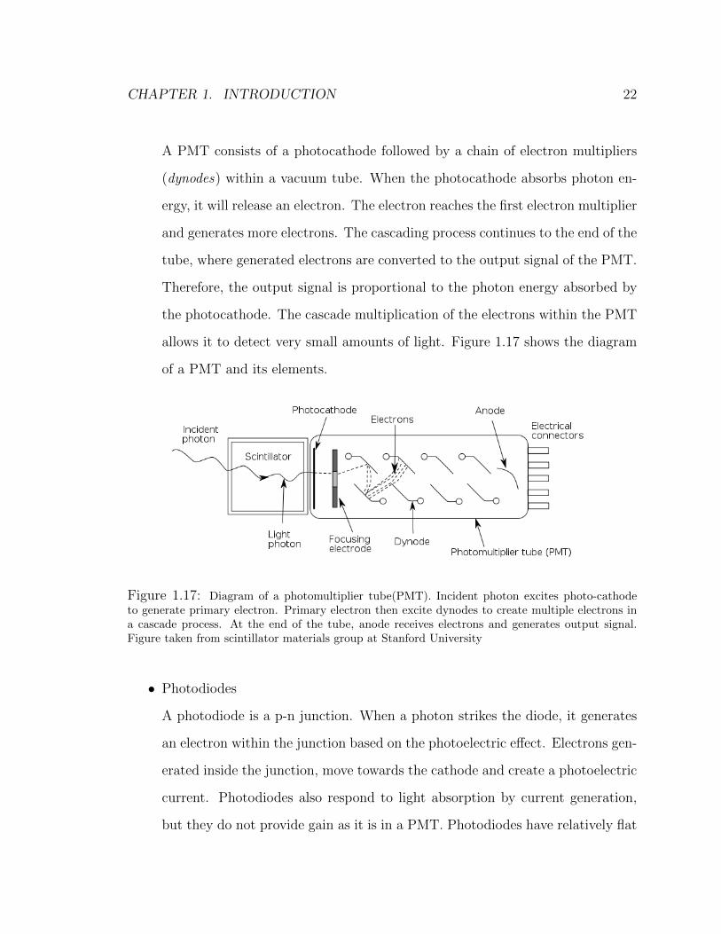
A PMT consists of a photocathode followed by a chain of electron multipliers
(dynodes) within a vacuum tube. When the photocathode absorbs photon en-
ergy, it will release an electron. The electron reaches the first electron multiplier
and generates more electrons. The cascading process continues to the end of the
tube, where generated electrons are converted to the output signal of the PMT.
Therefore, the output signal is proportional to the photon energy absorbed by
the photocathode. The cascade multiplication of the electrons within the PMT
allows it to detect very small amounts of light. Figure 1.17 shows the diagram
of a PMT and its elements.
Figure 1.17: Diagram of a photomultiplier tube(PMT). Incident photon excites photo-cathodeto generate primary electron. Primary electron then excite dynodes to create multiple electrons ina cascade process. At the end of the tube, anode receives electrons and generates output signal.Figure taken from scintillator materials group at Stanford University
• Photodiodes
A photodiode is a p-n junction. When a photon strikes the diode, it generates
an electron within the junction based on the photoelectric effect. Electrons gen-
erated inside the junction, move towards the cathode and create a photoelectric
current. Photodiodes also respond to light absorption by current generation,
but they do not provide gain as it is in a PMT. Photodiodes have relatively flat

CHAPTER 1. INTRODUCTION 23
response over the entire visible spectrum with high quantum efficiency. Their
uniform response, dynamic range and response speed are excellent. However,
they produce a considerable amount of noise, mostly thermal noise, resulting in
relatively poor signal-to-noise ratios. Avalanche photodiodes with limited gain
have been developed and been utilized in confocal and wide-field fluorescence
microscopes. Although they have up to 300-fold gain, they exhibit significant
dark noise even when cooled. Figure 1.18 compares quantum efficiency of the
two main types of the detectors.
Figure 1.18: Comparison of different detectors spectral sensitivity.

CHAPTER 1. INTRODUCTION 24
• Array Detectors
Most array detectors use semiconductor materials. Usually detector arrays con-
sist of small detector elements placed close to each other, each able to convert
the incident electromagnetic wave into an electrical signal. A circuit is attached
to each element to relay and multiplex the electrical signal to output amplifiers.
In our line scanning confocal microscope, we have used a CMOS linear array
detector which consists of photo-diode pixels. When one of these pixels, absorbs
a photon, the incident photon creates a hole and an electron in the semiconduc-
tor. Recombination of the electron and the hole generates the electrical signal.
The detection bandwidth of the detector array depends on the band gap en-
ergy of the semiconductor material since only photons that have energy higher
than the band gap energy of the semiconductor material can excite electrons
and create electron and hole. Hence the longest wavelength to be detected by
the detector is determined by the band gap energy of the semiconductor as in
Equation 1.4.
λcutoff =hc
Ebandgap=
1.24× 10⁻⁶(eV.m)
Ebandgap(eV )(1.4)
In most imaging applications, the range of wavelength to be detected is from
UV to IR, therefore, silicon with band gap energy of 1.1eV , is the the most
popular semiconductor for array detector for such applications. In our research,
the working wavelength is about 830nm, in near infra-red region. Hence, for
our line scanning confocal microscope a silicone linear array detector is used.
This is further discussed in Chapter 4.

Chapter 2
Light Sources
2.1 Introduction
The Light source is one of the most important components of an optical system.
Different modes of imaging require different light sources with different characteristics.
Therefore, based on the application, the light source is chosen. Properties such as
brightness, coherence and wavelength, are the most important properties that have to
be considered to choose a proper light source for an optical system. As in any other
engineering problem, these parameters are related to each other so there should be a
trade off among all these parameters. In the following sections, important properties
of a light source are discussed.
2.1.1 Brightness
The radiance theorem implies that the power emitted from a source element with a
projected area of dAproj into a solid angle of dΩ follows the relation with radiance of
the source as in Equation 2.1,
25

CHAPTER 2. LIGHT SOURCES 26
d2Φ = LdAprojdΩ, (2.1)
where d2Φ is the power in watts, dΩ is the solid angle and L is defined as the Radiance
of the source with the unit of (W/m2/sr). The theorem implies that, through a lossless
optical system, radiance is conserved [4]. In the other words, if an optical system does
not produce absorption and light undergoes perfect reflection and refraction while
going through the system, the radiance is conserved and is equal on source, specimen
and detector. Figure 2.1 illustrates the geometry for the radiance theorem.
Figure 2.1: Radiance in an Image. The image area is related to the object area by A2 = mA1,and the solid angles are related by Ω2 = Ω1
m2 ( nn′ )
2. Where m is the magnification and n and n′ arethe index of refraction of materials on two sides of the imaging system, respectively [4].
According to the radiance theorem, in microscopy, one of the most important
specifications of the light source is not only its ability to provide enough photons
per second, but also its ability to provide them from a small etendue. For instance,
a large fluorescent tube produces about the same number of photons per second
in comparison to the short arc HBO-50 bulb that is usually used in fluorescence

CHAPTER 2. LIGHT SOURCES 27
microscopy, but in the short arc HBO-50 bulb, this number of photons is produced
from an area about one million times smaller than the fluorescent tube. Therefore,
although the fluorescent tube and the short arc HBO-50 provide the same power, the
short arc HBO-50 provides higher radiance which is required in microscopy [5].
2.1.2 Wavelength
The other important feature of a light source is the light wavelength emitted from the
light source. Plasma and filament light sources which provide white light have almost
uniform spectra in visible wavelengths. Unlike them, arc sources produce photons
whenever an excited electron loses energy and moves to a lower energy level in the
material. Therefore, the wavelength of the light depends on the energy levels of the
electrons within the material. Based on Equation 2.2 and Equation 2.3 if the photon
in the visible spectrum is needed, then the difference of energy between each level
should be between 3.3 to 1.59 electron volts.
λ1 = 380nm⇒ E1 =hc
λ2= 3.26eV (2.2)
λ2 = 780nm⇒ E2 =hc
λ2= 1.59eV (2.3)
Traditionally, an efficient way to produce excited electrons from a small area is to
raise the temperature. This is usually done by heating tungsten filament or Hg or
Xe plasma. Figure 2.2 shows an emission spectrum of a Hg plasma. Peaks of the
spectrum represents different levels of excitation.

CHAPTER 2. LIGHT SOURCES 28
Figure 2.2: The emission profile of mercury arc lamp. Wavelengths in the visible region are usefulin fluorescence microscopy. Emission profile of the xenon arc lamp is presented. Xenon arc lampemission is almost flat in visible region [5].
2.1.3 Coherence
The other important property of a light source is its coherence. Coherence and
brightness are closely related to each other since most bright light sources tend to be
coherent. Brightness is the ability of the source to produce and focus a large number
of photons into a small focal spot. On the other hand, coherence is the ability of the
light source to generate photons that are in phase as a wave. Therefore, they interfere
constructively on the focal spot. Figure 2.3 illustrates the concept of temporal and
spatial coherence. It also shows how to make a coherent light source from an inco-
herent light source. Lasers produce not just one selected wavelength; they produce
a very narrow bandwidth. These wavelengths are coherent at the source, but after a
distance and scattered while passing through the optical system, these wavelengths
become no longer in phase with each other. These out-of-phase wavelengths interfere
with each other at the detector and produce a pattern of bright and dark spots on
the image called speckle.

CHAPTER 2. LIGHT SOURCES 29
Figure 2.3: Spatial coherence and temporal coherence. An incoherent light source emits light inall direction with different wavelengths. Waves that pass the pinhole aperture are spatially coherent,but in order to make a coherent beam, a wavelength filter is required. Figure taken from ZEISSmicroscopy online campus
Depending on the microscopy mode coherent or incoherent light sources offer
advantages. If the the microscope is working in reflectance or backscattered light
mode, utilizing a coherent light source will lead to speckle pattern generation in image.
On the other hand, for confocal microscopy we need high radiance for imaging since it
is required to focus the light onto a very small area on the specimen, and incoherent
light sources usually can not provide enough radiance. A trade off between these
two parameters usually results in choosing laser light sources for confocal microscopy.
There are of course exceptions of using non-laser light sources as discussed in the
following section.

CHAPTER 2. LIGHT SOURCES 30
2.2 Laser Light Sources
2.2.1 Introduction to Laser
In 1917, Albert Einstein established the foundation of light amplification by stim-
ulated emission of radiation (LASER). Basically, he re-derived Max Plank’s law of
radiation and predicted that, under certain conditions, a photon can stimulate an
excited atom in the material and generate a second photon with the exact same en-
ergy. This implies that the secondary photon has the same wavelength as the primary
photon. Also, the secondary photon would have the same phase, polarization and di-
rection of propagation. In the other words, the secondary photon is coherent with
the primary photon which results in a coherent beam.
A laser consists of a gain medium, a pumping mechanism and an optical feedback.
The gain medium is the material within the laser cavity. The pumping mechanism
excites atoms within the gain medium. When electrons from an excited atom return to
their stable level, they release the energy difference between energy levels in the form
of emission. Emitted photons are brought back to the cavity by the optical feedback
and stimulate more excited atoms in the gain medium, and, therefore, produce more
photons with the same phase and frequency. This process continues to amplify the
light. The output coupler is used to bring the laser beam to the optical system. The
wavelength of the beam mainly depends on the gain material and the cavity design.
Cavity design results output linewidth much smaller than material gain linewidth.
Most practical lasers contain additional elements that affect properties of the emitted
light such as the polarization, the wavelength, and the shape of the beam. Figure 2.4
represents a simple laser cavity with its components.

CHAPTER 2. LIGHT SOURCES 31
Figure 2.4: Laser cavity and lasing process. 1. Cavity consists of one fully reflective mirror, onepartly reflective mirror that couples the output beam to the optical system and gain medium. 2.Thepumping mechanism excites the atoms inside the gain medium. 3 to 5. Spontaneous emission causethe stimulated emission and lasing process continues to generate coherent laser beam.
Laser development rapidly increased the importance and the application of con-
focal microscopy. Lasers are easier to use and provide high radiance. The number of
excitation lines is increasing which provides a larger range of excitation especially in
fluorescence confocal microscopy. Lasers offer such good qualities as a light source,
which make them one of the most important and popular light sources being used
in confocal microscopy. Below, some of the most important properties of lasers are
discussed.
• Monochromaticity

CHAPTER 2. LIGHT SOURCES 32
Lasers provide a high degree of monochromaticity. Most of the time, it is
important to excite the specimen with a single wavelength. Usually light sources
provide a range of wavelengths. A smaller range of wavelengths leads to a higher
degree of monochromaticity, and it means that most of the excitation is done
by a single wavelength.
• Brightness
The term brightness is defined with different meanings in different textbooks. In
the context of lasers, brightness which is referred also as radiance is the power
divided by the area in the focus and the solid angle in the far-field. Therefore, its
unit is usually defined as watts per m2 per stradian (Wm−2sr−1). Lasers offer
higher radiance, which is very important in confocal microscopy. For lasers, the
solid angle Ω is defined as a function of the divergence half angle of the laser
(θ).
Ω = πθ2 (2.4)
For area (A) we have:
A = πw20 (2.5)
where w0 is the beam waist radius. Knowing that divergence angle of a laser is
θ = λπw0
for the AΩ product we have:
AΩ = πw20 × π
λ2
(πw0)2= λ2 (2.6)
Hence, for lasers, the radiance can be defined as in Equation 2.7,
L =Φ
λ2(2.7)

CHAPTER 2. LIGHT SOURCES 33
• Coherence
Coherence of two waves is defined as how well they are correlated and in phase.
In this term, light coming from lasers has both temporal and spatial coherence.
Temporal coherence implies that the wave is well correlated for all times. Spatial
coherence implies that the wave at different points in space is correlated. Spatial
coherence characteristic of lasers enable us to focus it onto a tight spot. This
is very important in confocal microscopy. Temporal coherence implies a very
narrow spectrum as stated in Equation 2.8.
δt
T=δz
λ≈ f
δf(2.8)
Equation 2.8 shows the relation between the coherence length and the linewidth
in wavelengths. For instance, for a laser with peak wavelength λ = 635nm
and with linewidth of δf = 20nm, coherence length is about 20 wavelengths.
Equation 2.8 implies that if δf decreases (narrow bandwidth), the coherence
length increases.
In addition, some types of lasers provide plane polarized emission, and they usually
provide a Gaussian beam profile. Based on the output power profile of the laser, we
can classify lasers as two main types of Continuous Wave or Pulsed.
• Continuous Wave Laser
As the name states, continuous wave lasers provide continuous output power
over time. Figure 2.5 represents the output power profile for both continuous
and pulsed lasers. Theoretically, a continuous wave laser can be used to gen-
erate pulses of light. We can intentionally switch a continuous wave laser on
and off to generate a beam in pulsed form. Basically a continuous wave laser

CHAPTER 2. LIGHT SOURCES 34
is continuously pumped, therefore, a continuous wave laser provides constant
power over time which is essential in some applications to have constant power.
Continuous wave lasers work in either single-mode or multi-mode. Single-mode
operation implies that laser linewidth is very small which results in long co-
herence length. On the other hand, multi-mode operation implies that the the
laser linewidth is multiple of the mode spacing of the laser resonator, which
provides wider range of wavelengths and shorter coherence length.
• Pulsed Laser
Generally, other types of lasers that are not continuous wave laser are classified
as pulsed operation lasers. Therefore, their output power appears to be in the
form of pulses of different duration and different frequency. Some lasers are
classified as pulsed just because they cannot work in a continuous wave mode.
On the other hand, in some applications it is required to expose a sample to
a large amount of power. Energy within a pulse is equivalent to the average
power divided by the pulse repetition frequency.
In some other applications, the amount of energy in the pulse is not important
but the peak of pulse power is required. This is usually required in nonlinear
optics effects. In this case, generating short time pulses is important. There are
techniques to make pulse duration as short as possible for these types of appli-
cations. Figure 2.5 represents typical output power profile for both continuous
and pulsed laser.

CHAPTER 2. LIGHT SOURCES 35
Figure 2.5: Power profile of two classes of lasers. Although the average power of both profiles arethe same, but the pulsed laser contains higher power within a very small period of time, whereas inthe continues wave laser the output power is constant for all the time.
2.2.2 Laser Diode
Our research is focused on confocal microscopy. As mentioned in Chapter 4, we have
used a continuous wave laser diode with wavelength λ = 830nm as the light source for
both line scanning and point scanning confocal microscopes. As stated in previous
section, a laser consists of a gain medium and a pumping system. A laser diode
uses semiconductor materials to create p-n junction like a light emitting diode, as
the medium. In laser diodes, the gain medium is pumped electronically. Applying
voltage to the semiconductor p-n junction will create electrons and holes. As in
light emitting diodes, recombination of the electrons and holes generates photons. In

CHAPTER 2. LIGHT SOURCES 36
laser diodes, the goal is to recombine electrons and holes in the intrinsic region. This
semiconductor structure is located inside a laser cavity, to create laser diodes. Typical
materials being used in laser diode structure are Ga, In,Al, As, P and N. Different
combination of these materials provide different wavelength for the laser diode. For
instance, in order to obtain wavelength in the near infrared region, GaAlAs or GaAs
are typical combinations and for infra red region, InP or InGaAsP are combinations
typically being used. Laser diodes are usually small in size and therefore easy to use
in optical systems. Besides, they provide large variety of wavelengths.
2.3 Non-Laser Light Sources
Confocal microscopy was invented before the invention of laser. Early confocal mi-
croscopes used non-laser light sources. Although a laser is the favorite light source
in confocal microscopy, it has some disadvantages which open the way for non-laser
light sources in confocal microscopy. As discussed, because of the high degree of
coherence in lasers they provide high radiance required in confocal microscopy, but
their high degree of coherence leads to speckle pattern in the image. Therefore, in-
coherent light sources or in general, non-laser light sources have this advantage over
laser light sources. Two main class of non-laser light sources such as arc lamps and
light emitting diodes (LED) are described in the following sections.
2.3.1 Arc Lamps
Light produced by arc lamps is based on electric discharge between two piece of metal
known as the cathode and anode. The cathode and anode are placed close to each
other. Applying a large electrical voltage across the cathode and anode results in
CHAPTER 2. LIGHT SOURCES 37
an electrical discharge and ionization of the gas between them. When the electron
of the excited atom returns to its stable level, it releases the energy in the form of
light. The wavelength of the emitted photon depends on the electron energy levels in
atoms of the gas between the cathode and anode. Usually arc lamps are named after
the gas in between the cathode and anode. Neon, xenon and mercury are examples
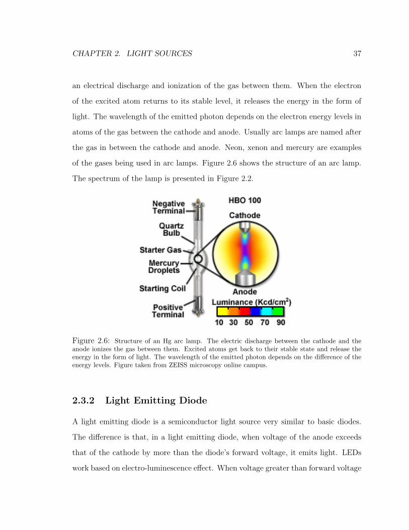
of the gases being used in arc lamps. Figure 2.6 shows the structure of an arc lamp.
The spectrum of the lamp is presented in Figure 2.2.
Figure 2.6: Structure of an Hg arc lamp. The electric discharge between the cathode and theanode ionizes the gas between them. Excited atoms get back to their stable state and release theenergy in the form of light. The wavelength of the emitted photon depends on the difference of theenergy levels. Figure taken from ZEISS microscopy online campus.
2.3.2 Light Emitting Diode
A light emitting diode is a semiconductor light source very similar to basic diodes.
The difference is that, in a light emitting diode, when voltage of the anode exceeds
that of the cathode by more than the diode’s forward voltage, it emits light. LEDs
work based on electro-luminescence effect. When voltage greater than forward voltage

CHAPTER 2. LIGHT SOURCES 38
drop is applied to the LED, current flows and electrons start to move and combine
with holes. This recombination releases energy e·Vg, where Vg is the band gap voltage
of the LED and e is the electron charge. This energy determines the frequency and
therefore wavelength of the emitted photon. Figure 2.7 shows the structure of a LED
and how electrons flow through the junction, recombine with holes and emit photon.
As incoherent light sources, LEDs are important because of their long life and high
efficiency which make them favorite in so many applications such as traffic lights.
Figure 2.7: Diagram of a light emitting diode. Applying voltage to the LED will results in currentflow within the junction. When electrons recombine with holes, they release their energy in the formof light. This phenomenon is called electro-luminescence effect. Figure taken from Department ofPhysics at Warwick University.
In microscopy, especially in confocal microscopy, a high brightness light source
is needed. Although high power LEDs have been developed that can provide high
power. They achieve high power because of their large area therefore, they can not
provide enough radiance required for confocal imaging. Recently, high brightness
LEDs have been developed which are discussed in the following section.

CHAPTER 2. LIGHT SOURCES 39
2.3.3 High Brightness LED
High power LEDs have different application due to their high power and lifetime.
They are being used in room lighting, mobile lighting and so many applications. But
as discussed before, high power is not enough for microscopy. Especially in confocal
microscopy where it is required to focus light onto a diffraction limited spot, high
brightness sources play a critical role. Recently, high brightness LEDs have been
developed. Not only, they can produce a large number of photons per second, but
also they can provide this large number of photons per second from a very small area.
For the first time in confocal microscopy, we have used a high brightness LED in our
line scanning confocal system. Specifications of the LED that we used, are presented
in more details in Chapter 4 with the experimental results.
2.4 Summary
In this chapter, we have discussed general properties of a light source proper for
confocal microscopy. We discussed laser and non-laser light sources. We have used
a continuous wave laser diode and a high brightness LED in our experiments. Tabel
2.1 summarize main properties of typical light sources.
Spectral Range Power Radiance (W/m2/sr) LinewidthTungsten 360− 1000nm ≈ 6× 10⁵ wide
Hg Arc (HBO50) 250− 600nm 50W ≈ 4× 10⁷ wideLaser Diode 830 nm 24 mW 3.5× 10¹⁰ ≈ 1nm
HE-NE Laser 632 nm ≈ 50mW 1.25× 10¹¹ 0.01 nmHB LED 750-850 nm 30 mW ≈ 9.6× 10³ 32 nm
LDLS 170 - 800 nm ≈ 5× 10⁶(λ = 500nm) wide
Table 2.1: Summary of light sources properties for different light sources..

Chapter 3
Scattering Medium and Pupil
Configurations
3.1 Scattering Media and Gating Mechanism
Generally, the goal in imaging is to capture specific photons coming from the speci-
men to form the image. Multiply scattered photons, which are generally unwanted,
can reach the detector and contribute in the image formation. A multiply scattered
photon is defined as a photon which originates from somewhere other than the imag-
ing area of interest, having been scattered multiple times. Usually, the detector is
focused so that it detects photons coming from the area of interest. However, some
of the multiply scattered photons reaches the detector. These photons contribute
destructively in the image formation and reduce contrast and resolution of the image.
Figure 3.1 shows how multiple scattered photons can reach the detector and cause
image degradation.
In most biomedical applications, the medium is highly scattering. For instance,
40
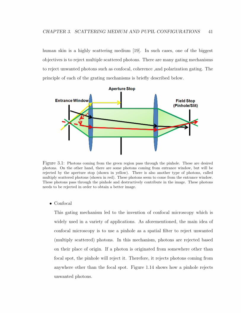
CHAPTER 3. SCATTERING MEDIUM AND PUPIL CONFIGURATIONS 41
human skin is a highly scattering medium [19]. In such cases, one of the biggest
objectives is to reject multiple scattered photons. There are many gating mechanisms
to reject unwanted photons such as confocal, coherence ,and polarization gating. The
principle of each of the grating mechanisms is briefly described below.
Figure 3.1: Photons coming from the green region pass through the pinhole. These are desiredphotons. On the other hand, there are some photons coming from entrance window, but will berejected by the aperture stop (shown in yellow). There is also another type of photons, calledmultiply scattered photons (shown in red). These photons seem to come from the entrance window.These photons pass through the pinhole and destructively contribute in the image. These photonsneeds to be rejected in order to obtain a better image.
• Confocal
This gating mechanism led to the invention of confocal microscopy which is
widely used in a variety of applications. As aforementioned, the main idea of
confocal microscopy is to use a pinhole as a spatial filter to reject unwanted
(multiply scattered) photons. In this mechanism, photons are rejected based
on their place of origin. If a photon is originated from somewhere other than
focal spot, the pinhole will reject it. Therefore, it rejects photons coming from
anywhere other than the focal spot. Figure 1.14 shows how a pinhole rejects
unwanted photons.
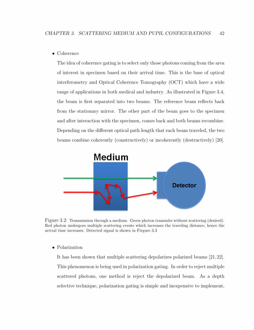
CHAPTER 3. SCATTERING MEDIUM AND PUPIL CONFIGURATIONS 42
• Coherence
The idea of coherence gating is to select only those photons coming from the area
of interest in specimen based on their arrival time. This is the base of optical
interferometry and Optical Coherence Tomography (OCT) which have a wide
range of applications in both medical and industry. As illustrated in Figure 3.4,
the beam is first separated into two beams. The reference beam reflects back
from the stationary mirror. The other part of the beam goes to the specimen
and after interaction with the specimen, comes back and both beams recombine.
Depending on the different optical path length that each beam traveled, the two
beams combine coherently (constructively) or incoherently (destructively) [20].
Figure 3.2: Transmission through a medium. Green photon transmits without scattering (desired).Red photon undergoes multiple scattering events which increases the traveling distance, hence thearrival time increases. Detected signal is shown in Firgure 3.3
• Polarization
It has been shown that multiple scattering depolarizes polarized beams [21,22].
This phenomenon is being used in polarization gating. In order to reject multiple
scattered photons, one method is reject the depolarized beam. As a depth
selective technique, polarization gating is simple and inexpensive to implement,

CHAPTER 3. SCATTERING MEDIUM AND PUPIL CONFIGURATIONS 43
Figure 3.3: Arrival time for photons shown in Figure 3.2. Green signal corresponds to transmittedphotons without scattering. Red signal corresponds to multiply scattered photons reached thedetector traveled longer distance. The detector is turned on for the gating window, therefore, redsignal is rejected.
but it is unable to provide deep penetration detection. Figure 3.5 shows how
a polarizer transmits a specific polarization and reject the rest of the incident
beam. This phenomenon is the base of polarization gating.
Rejecting unwanted photons can considerably increase image contrast as is shown
in Figure 3.6. The image to the left is captured without using a polarizer. Knowing
that most of the light reflected from the surface of the water is S polarized, one can
reject the specular reflection form the surface of the water by utilizing a polarizer
that blocks S polarization.

CHAPTER 3. SCATTERING MEDIUM AND PUPIL CONFIGURATIONS 44
Figure 3.4: Basics of interferometry. Based on the optical path length, beams from reference andsource arms interfere constructively (on the right) or destructively (on the left).
3.2 Pupil Configurations
As discussed, rejecting more of the multiple scattered photons leads to image improve-
ment. We have utilized different pupil configurations for our line scanning confocal
microscope in order to study the effect of different pupil configurations on rejecting
unwanted photons. In the following three sections, we have discussed full pupil config-
uration as the most popular configuration. It utilizes the whole numerical aperture of
the objective. Our goal is to study divided pupil configuration and compare it to full
pupil configuration. In divided pupil configuration, half of the numerical aperture is
being used, therefore we lose resolution, but it is able to reject more of the unwanted
photons. As an intermediate step between full pupil configuration and divided pupil
configuration, we have discussed half pupil configuration.
3.2.1 Full Pupil Configuration
In general, most microscopes use the full pupil aperture for both illumination and
detection. In the case of confocal microscopy, a high numerical aperture objective
lens is required. As mentioned earlier in Equations 1.1 and 1.3, it is critical to use full

CHAPTER 3. SCATTERING MEDIUM AND PUPIL CONFIGURATIONS 45
Figure 3.5: Polarization gating. Light coming from the light source is unpolarized. After it passesthrough the polarizer, only the portion of the light that its polarization matches with the polarizersorientation goes through. In case of microscopy and rejecting multiple scattered photons, the lightcoming from the specimen is deplorized after multiple scattering events. Therefore, by utilizing apolarizer with the right orientation, one can reject unwanted photons. Figure taken from AmericanPolarizers Inc. website.
numerical aperture in order to obtain a good lateral and axial resolution. Although
using the full numerical aperture provides better resolution, it will collect more of
the unwanted multiple scattered photons which degrade the image. Since, confocal
microscopy requires high numerical aperture, we have used an oil immersed objective
lens with NA = 0.9 and 60X magnification. Resolution measurements has been
done and is discussed in Chapter 4. Figure 3.7 shows how utilizing the full pupil
configuration leads to gathering more of the unwanted multiple scattered photons.

CHAPTER 3. SCATTERING MEDIUM AND PUPIL CONFIGURATIONS 46
Figure 3.6: Image of the surface of the water. Reflection form the surface of the water is Spolarized. In order to reject the S polarization, a polarizer is used (image on the right) whichimproves the contrast.
3.2.2 Half Pupil Configuration
As stated, the full pupil configuration provides good resolution since it utilizes the
full numerical aperture of the objective lens, but it collects more of the unwanted
multiple scattered photons. In comparison to the full pupil configuration, the half
pupil configuration is more successful in rejecting unwanted photons, but in the case
of the half pupil configuration, microscope uses only half of the numerical aperture
of the objective lens. Based on Equations 1.1 and 1.3, the half pupil configuration
loses lateral and axial resolution by a factor of two and four, respectively. Therefore,
by utilizing the half pupil configuration, more of the unwanted photons are rejected,
but this is done with the cost of losing lateral and axial resolution.
3.2.3 Divided Pupil Configuration
We have established that the full pupil configuration provides better resolution in
comparison to the half pupil configuration. Koester et al. proposed a combination of

CHAPTER 3. SCATTERING MEDIUM AND PUPIL CONFIGURATIONS 47
Figure 3.7: Multiple scattering photons in full pupil and half pupil configuration. It is shown thatin full pupil configuration (on the left), unwanted multiple scattered photons can pass through thewhole pupil. In case of using the half pupil configuration (on the right), statistically, half of theeunwanted multiple scattered photons is rejected by pupil stop ,but it leads to losing resolution sinceonly half of the numerical aperture is being used.
the full pupil and half pupil configurations that can provide benefits of both config-
urations [23, 24]. The divided pupil configuration uses half of the objective aperture
for illumination and the other half for detection. Therefore, paths for the incident
and the reflected beams are completely separate. As reported, although utilizing half
the numerical aperture will reduce lateral and axial resolution, divided pupil config-
uration can recover some of the lost resolution by rejecting more of the unwanted
photons [25]. Figure 3.8 represents divided pupil configuration proposed by Koester
et al.
The divided pupil configuration has been used in line scanning confocal micro-
scopes for imaging human tissue [26]. We are going to discuss more about the divided
pupil configuration in Chapter 4 since we have used the divided pupil configuration
in our line scanning confocal microscope.

CHAPTER 3. SCATTERING MEDIUM AND PUPIL CONFIGURATIONS 48
Figure 3.8: Divided pupil configuration uses half of the pupil for illumination and the otherhalf for detection. Multiple scattered photons are drawn for two cases. In case (a) the photondoes not contribute in the image since it is not in the illumination path. In case (b) the photonreaches the detector. Therefore, statistically, divided pupil configuration works the same as halfpupil configuration in terms of rejecting unwanted multiple scattered photons.
3.2.4 Comparison
Qualitatively, we mentioned that the full pupil configuration provides the best reso-
lution in between the three discussed configurations, but it is weak in the background
rejection. Therefore, in terms of resolution, it is expected that the full pupil configu-
ration works the best and the divided pupil configuration is better than the half pupil
configuration. Studies on line scanning microscope have proved the above theory.
Gareau et al. used the line scanning confocal microscope for imaging the epidermis
in human skin. It is reported that the divided pupil configuration provides lateral
resolution and sectioning ability comparable with point scanning system. Table 3.1
represent results reported by Gareau et al [27]. Later in the chapter 4, in our experi-
ments, we have reported our results for both divided and full pupil configurations in
line scanning confocal microscope. Our results are consistent with results published

CHAPTER 3. SCATTERING MEDIUM AND PUPIL CONFIGURATIONS 49
by Gareau et al.
Axial resolution Lateral ResolutionFull Pupil 1.7± 0.1µm 0.8± 0.1µm
Divided Pupil 1.7± 0.1µm 1± 0.1µm
Table 3.1: Comparison between full pupil configuration and divided pupil configuration on theline scanning confocal microscope as reported by Gareau et al [27].
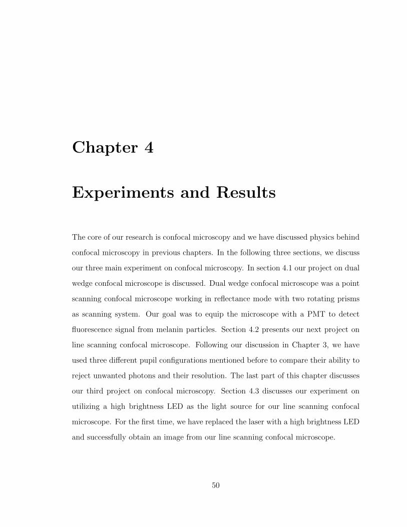
Chapter 4
Experiments and Results
The core of our research is confocal microscopy and we have discussed physics behind
confocal microscopy in previous chapters. In the following three sections, we discuss
our three main experiment on confocal microscopy. In section 4.1 our project on dual
wedge confocal microscope is discussed. Dual wedge confocal microscope was a point
scanning confocal microscope working in reflectance mode with two rotating prisms
as scanning system. Our goal was to equip the microscope with a PMT to detect
fluorescence signal from melanin particles. Section 4.2 presents our next project on
line scanning confocal microscope. Following our discussion in Chapter 3, we have
used three different pupil configurations mentioned before to compare their ability to
reject unwanted photons and their resolution. The last part of this chapter discusses
our third project on confocal microscopy. Section 4.3 discusses our experiment on
utilizing a high brightness LED as the light source for our line scanning confocal
microscope. For the first time, we have replaced the laser with a high brightness LED
and successfully obtain an image from our line scanning confocal microscope.
50

CHAPTER 4. EXPERIMENTS AND RESULTS 51
4.1 Dual Wedge Confocal Microscope
As mentioned in previous chapters, point scanning confocal microscopy requires scan-
ning in two dimensions. It can be done either by scanning the beam on the specimen
or moving the specimen with stationary beam. Besides the cost and complexity of
utilizing two scanners, it leads to lower frame rate, specially if the field of view is big.
Dual wedge scanning reflectance confocal microscopy is designed to overcome these
problems. Instead of two mirror scanners, it utilizes two rotating prisms to scan the
beam on the specimen. This is an easy process to find the location of the scanned
spot, although we lose the uniformity in scanning area. the following section discuss
our research on point scanning confocal microscope with dual wedge scanning system.
4.1.1 Dual Wedge Scanner
The dual wedge scanner was a point scanning confocal microscope working in re-
flectance mode designed by Warger et al [6]. The goal behind designing the dual
wedge confocal microscope was to scan the field of view faster and easier in compar-
ison to other scanning systems. As discussed, in general point scanning microscope,
two scanners scan the beam on the specimen in two dimensions, which requires more
space and also costs more. The dual wedge scanner has the same basic components
of a reflectance confocal microscope except for the scanning system. The scanning
system consists of two prisms back to back on their bases. As illustrated in Figure 4.1,
a beam passing through one prism refracts due to mismatch in the index of refraction
between the prism and air. The angle of refraction depends on indices of refraction
and the prism apex angle (α). Now if the prism rotates, the beam starts to rotate
on the pattern as in Figure 4.1 (a). If two prisms placed back to back on their bases,

CHAPTER 4. EXPERIMENTS AND RESULTS 52
are used in front of the beam, depending on their speed and direction of rotation, the
beam travels in different patterns.
Figure 4.1: Basic of the dual wedge scanning system. (a) Refraction by one prism. Rotating theprism will cause the beam to travel a circular pattern. (b) Refraction by two rotation prism. Eachprism will generate a circular pattern. (c) Combination of the patterns. Based on the direction andspeed of rotation, different patterns of scanning can be obtained [6].
Figure 4.2 shows two different scanning patterns of the dual wedge reflectance
confocal microscope scanner. If the prisms rotate in the same direction, scanning
pattern (a) is obtained, and if the prisms rotate in the opposite directions, pattern
(b) is achieved for scanning.
Pattern (a) in Figure 4.2 covers mostly the surrounding area of the field of view
and pattern (b) covers mostly the center area of the field of view. In either case, the
dual wedge does not uniformly scan the whole field of view. Considering that the dual

CHAPTER 4. EXPERIMENTS AND RESULTS 53
Figure 4.2: Two general patterns of scanning. (a) is achieved when prisms rotate in the samedirection. (b) is achieved when prisms rotate in the opposite direction [6].
wedge scanning system is much cheaper and easier to use in comparison to the raster
scan with two scanner, we sacrifice uniformity in the scanning area to achieve a faster
and simpler scanning system. Two motors are connected to the Labview software,
and their phase, and speed of rotation are controlled by the computer. Also, a data
acquisition card is connected to the software. Therefore, based on the position of
prisms, software detects the position of the scanning spot in the field of view. The
image of the field of view forms based on the position of the scanning spot and data
collected from the detector at the right time. Figure 4.3 shows a sketch of the dual
wedge confocal microscope. The microscope works in reflectance mode. The beam
from the laser diode with λ = 839nm goes through the polarizing beam splitter. The
beam then goes through a Rayleigh pair to the quarter wave plate. The quarter
wave plate changes the polarization of the beam from linear polarization to circular
polarization. Reflected light from the sample is gathered by the objective lens. The
reflected beam travels the same path to the polarizing beam splitter. Since the speed
of light is much higher than the prisms’ speed of rotation, the prisms de-scan the

CHAPTER 4. EXPERIMENTS AND RESULTS 54
reflected beam. The reflected beam is assumed to consist only the photons that have
been scattered once. Therefore, the reflected beam is still circularly polarized. After
the reflected beam has passed the quarter wave plate the second time, its polarization
is perpendicular to that of the incident beam. Hence the polarizing beam splitter
reflects the de-scanned beam to the detector. A lens focuses the de-scanned beam
onto the pinhole confocal to the focal spot on the specimen. The avalanche photodiode
converts the beam into an electrical signal which is then converted into digital data
that represents the brightness of the scanned spot on the specimen.
Figure 4.3: Diagram of the dual wedge scanning reflectance confocal microscope.
Figure 4.4 shows images taken by the dual wedge scanning reflectance confocal
microscope as reported by Warger et al.
4.1.2 Fluorescence Modes
The microscope designed and built by Warger et al. was working only in reflectance
mode. In our project, we wanted to add a fluorescence detection mode to the setup.
The goal was to use a continuous wave laser diode to excite the melanin molecule
stepwise and detect the fluorescence signal utilizing a photomultiplier tube. Melanin
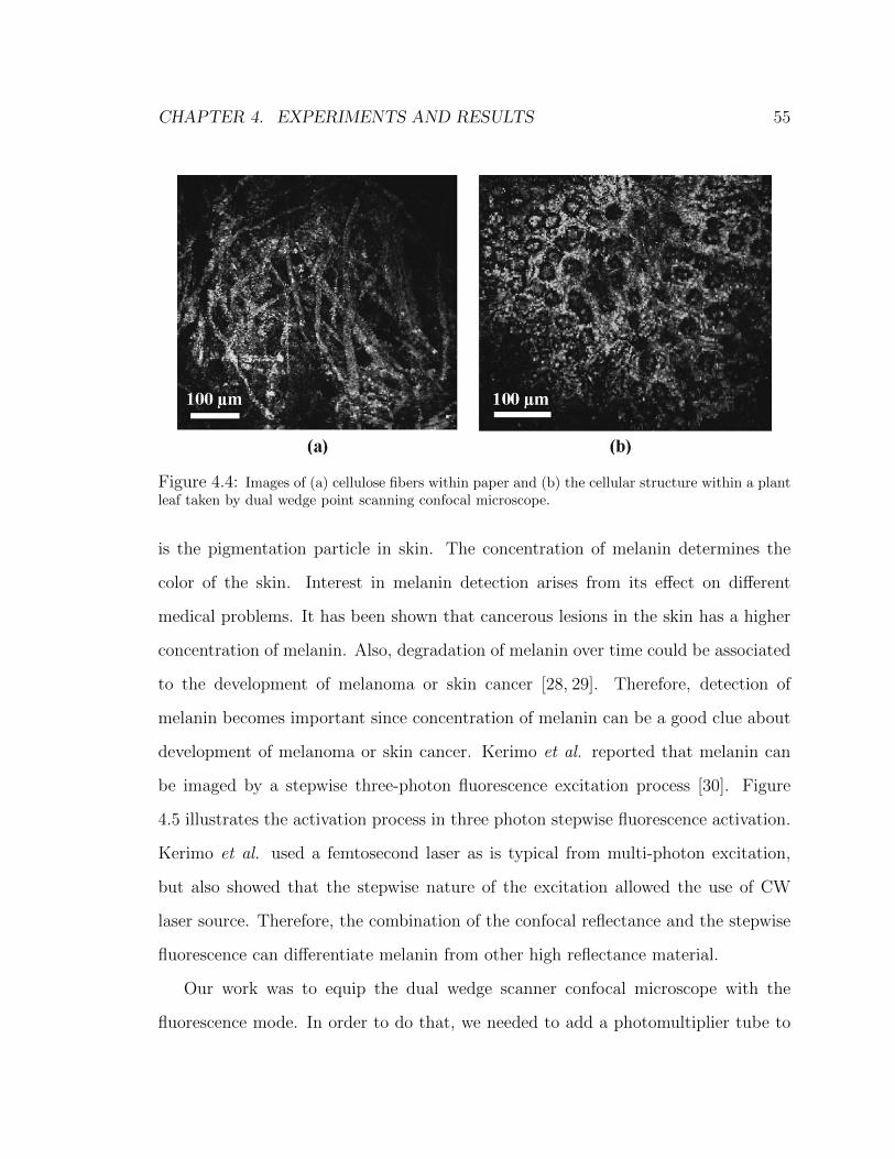
CHAPTER 4. EXPERIMENTS AND RESULTS 55
Figure 4.4: Images of (a) cellulose fibers within paper and (b) the cellular structure within a plantleaf taken by dual wedge point scanning confocal microscope.
is the pigmentation particle in skin. The concentration of melanin determines the
color of the skin. Interest in melanin detection arises from its effect on different
medical problems. It has been shown that cancerous lesions in the skin has a higher
concentration of melanin. Also, degradation of melanin over time could be associated
to the development of melanoma or skin cancer [28, 29]. Therefore, detection of
melanin becomes important since concentration of melanin can be a good clue about
development of melanoma or skin cancer. Kerimo et al. reported that melanin can
be imaged by a stepwise three-photon fluorescence excitation process [30]. Figure
4.5 illustrates the activation process in three photon stepwise fluorescence activation.
Kerimo et al. used a femtosecond laser as is typical from multi-photon excitation,
but also showed that the stepwise nature of the excitation allowed the use of CW
laser source. Therefore, the combination of the confocal reflectance and the stepwise
fluorescence can differentiate melanin from other high reflectance material.
Our work was to equip the dual wedge scanner confocal microscope with the
fluorescence mode. In order to do that, we needed to add a photomultiplier tube to

CHAPTER 4. EXPERIMENTS AND RESULTS 56
Figure 4.5: Fluorescence process. In 1-photon fluorescence, electron absorbs a photon and goesto a higher level of energy. This is a real state. The excited electron returns to its stable level andemit a photon with slightly higher wavelength in comparison to the primary photon. In 3-photonexcitation, electron absorbs 3-photon and stepwise. It can go up to three real states as in the ploton the right. In our case, the melanin can absorb three photon and stepwise go up three virtualstates and then emit a photon.
detect the weak fluorescence signal. Slight modifications and new design were done
as shown in Figure 4.6. The quarter wave plate is part of the reflectance mode,
therefore, in order to detach it from fluorescence mode, it was relocated to in front of
the polarizing beam splitter. The Rayleigh telescope was modified to match the lens
in front of the detector.
The PMT used was a Hamamatsu 3907-03, which displays a fairly high sensitivity
even into the NIR region. The high sensitivity of the PMT in the NIR region can
be problematic for imaging the fluorescence. Even a small fraction of the laser light,
reflected from the dichroic to the PMT, could be more intense than the three-photon
fluorescence. This would have limited the specificity of the PMT signal to the three-
photon fluorescence. To overcome this problem, an 800nm short-pass filter was added
in front of the PMT. The filter was verified to be robust enough to block the laser
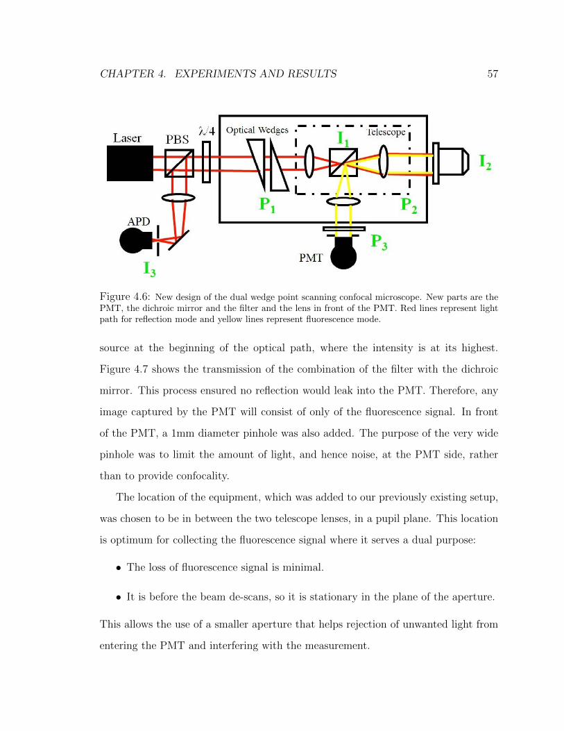
CHAPTER 4. EXPERIMENTS AND RESULTS 57
Figure 4.6: New design of the dual wedge point scanning confocal microscope. New parts are thePMT, the dichroic mirror and the filter and the lens in front of the PMT. Red lines represent lightpath for reflection mode and yellow lines represent fluorescence mode.
source at the beginning of the optical path, where the intensity is at its highest.
Figure 4.7 shows the transmission of the combination of the filter with the dichroic
mirror. This process ensured no reflection would leak into the PMT. Therefore, any
image captured by the PMT will consist of only of the fluorescence signal. In front
of the PMT, a 1mm diameter pinhole was also added. The purpose of the very wide
pinhole was to limit the amount of light, and hence noise, at the PMT side, rather
than to provide confocality.
The location of the equipment, which was added to our previously existing setup,
was chosen to be in between the two telescope lenses, in a pupil plane. This location
is optimum for collecting the fluorescence signal where it serves a dual purpose:
• The loss of fluorescence signal is minimal.
• It is before the beam de-scans, so it is stationary in the plane of the aperture.
This allows the use of a smaller aperture that helps rejection of unwanted light from
entering the PMT and interfering with the measurement.

CHAPTER 4. EXPERIMENTS AND RESULTS 58
Figure 4.7: Transmission of the filter in front of the PMT and reflection of the dichroic mirror.The goal was to block any leak from the incident beam to the PMT. The fluorescence wavelength isabout 450nm. The spectrum of the combination of the filter and the dichroic mirror shows that wewere successful in rejecting 839nm wavelength of the laser.
4.1.3 Results
The laser power at the sample was measured to be about 0.5mW . This power is
enough to activate the melanin particles in order to see the enhanced melanin emission
[30]. Figure 4.8 shows the images obtained from both confocal reflectance and three-
photon fluorescence modalities, as well as the merged image of the two modalities
(Figure 4.8 (a), (b), and (c) respectively). It can be seen from the images that even
in confocal reflectance mode, pure melanin strongly reflects the NIR light. In Figure
4.8(b) the background information is completely suppressed, and only fluorescence
from specific areas containing melanin is observed. From the merged image, it can be
seen that the locations that exhibit high three-photon emission are perfectly registered

CHAPTER 4. EXPERIMENTS AND RESULTS 59
to the location of the melanin particles.
Figure 4.8: Images of enhanced emission of Sepia melanin in atmosphere. (a) confocal reflectanceimage. (b) three-photon image. (c) merged image. Scale bar is 10µm
The suppression of all background information, when switching between confocal
reflectance and three-photon fluorescence mode, suggests that the origin of the signal
is indeed the step-wise fluorescence process. This background suppression was only
possible after adding the filter in front of the PMT. Prior to having the additional
filter, the image included the USAF target. This resulted from the very small amount
of reflected IR light that entered the PMT. This image provided the same information
as confocal reflectance, however, without the sectioning ability. That image was also
lacking the needed specificity to melanin. Similarly, Figure 4.9 displays a series of
images in the same order as in Figure 4.8, but of a dark human hair instead of melanin
particles. In this case as well, the location of the fluorescence is perfectly aligned with
the location of the hair sample, and no signal was seen elsewhere, where melanin is not
present. In order to better demonstrate the fluorescence using the hair sample, the
confocal image, Figure 4.9(a), and the three-photon excitation emission Figure 4.9(b)
are slightly misplaced along the optical axis. By focusing the confocal reflectance
on the substrate, the hair appears darker than the background. The fluorescence
image remained focused on the hair. Therefore, when merging the confocal with the
CHAPTER 4. EXPERIMENTS AND RESULTS 60
excited fluorescence images, the fluorescence sites will have a better contrast and help
demonstrate the phenomenon. As can be seen from Figure 4.8 and Figure 4.9, both in
the case of pure melanin particles from Sepia and the case of melanin from the human
hair sample, not all areas that appear to have melanin present actually demonstrate
three-photon fluorescence.
Figure 4.9: Images of a dark human hair in atmosphere. (a) confocal reflectance image. (b)three-photon image. (c) merged image. Scale bar is 10µm.
In Figure 4.8, the pure melanin case, some of the melanin particles stuck to the
cover-slip, while others remained on the surface of the USAF target. The gap between
the two surfaces can very easily exceed 20µm, which is approximately the length of
the excited volume along the focal axis. Therefore, some regions will remain outside of
this focal volume, where the three-photon fluorescence excitation is generated. These
regions correspond with particles that did not appear to be emitting any fluorescence
when switching modalities. In the human hair case of Figure 4.9, the sample was not
held under a cover-slip. In this case, however, changes along the focal axis, which
occurred due to the wavy nature of the hair will have the same effect. In addition, the
melanin distribution inside the focused region, is in the form of spot shaped clusters,
as typical to the distribution of melanin in the hair.

CHAPTER 4. EXPERIMENTS AND RESULTS 61
4.1.4 Conclusion
The three photon stepwise fluorescence was previously observed by Kerimo et al.,
but in this project, we were able to activate the process using a continuous wave
laser with dual wedge confocal microscope which is much cheaper and easier to use.
We have shown that a melanin-specific fluorescence channel can be easily added to a
reflectance confocal microscope. We were able to image melanin fluorescence in both
pure melanin and human hair. Results that our dual wedge scanner setup is able to
detect melanin in both reflectance and fluorescence modes.
4.2 Line Scanning Confocal Microscope
We have discussed that point scanning systems require scanning systems in two di-
mensions which makes the data acquisition time slower and adds to the complexity of
the system. Besides good resolution, in-vivo imaging requires faster image formation.
One way to form the image faster is to use line scanning confocal. Although line
scanning is confocal in only one direction, it provides comparably good resolution.
On the other hand, in reflectance confocal microscopy, we are interested in single
scattered photons. Photons that undergo many scattering effects do not provide in-
formation from the interest area of imaging. In order to study the effect of different
pupil configurations in rejecting unwanted multiply scattered photons, we have used
3 different pupil configurations on line scanning confocal microscope. The following
section represents our study on different pupil configurations.

CHAPTER 4. EXPERIMENTS AND RESULTS 62
4.2.1 Instrumentation
The advantage of using the line scanning confocal microscope is that it is faster,
much cheaper and easier to work with. Besides dealing with a more complicated
system, the points scanning confocal microscope with two scanners costs more. One
way to simplify the system is to use one scanner and instead of working in the point
scanning mode, work in the line scanning mode. The microscope was previously
designed by Dwyer et al. [3]. In our project, the main goal was to try different pupil
configurations and measure the lateral and the axial resolution of the line scanning
confocal microscope for each pupil configuration. In order to study different pupil
configurations, our setup has multiple image and pupil planes. Figure 4.10 shows
the schematic of the microscope. Note the image and pupil planes that have been
distinguished by different numbers. Aperture stops were applied on pupil planes 1
and 3 for the illumination and the receiving paths respectively.
The light source is a laser diode with the wavelength of 830nm. The beam passes
through the cylindrical lens that focuses it onto a line on pupil plane 1. Then the
beam splitter reflects half of the beam to the Rayleigh pair with unity magnifica-
tion. On pupil plane 2, a galvanometric scanner sweeps the beam on the sample to
scan the field of view (FOV). The beam then goes through another Rayleigh pair
with unity magnification which focuses it onto the back focal plane of the objective
lens. The objective lens is an Olympus LUMPlanFI/IR, 60X, NA=0.90, water im-
mersion objective lens. It focuses the beam onto a line on the sample and collects
the backscattered light. The back scattered light goes through the Rayleigh pair to
the galvo. The galvo de-scans the backscattered light. Half of the backscattered light
passes the beam splitter. A lens in front of the detector is used to focus the back
scattered light on the line detector. The detector is a linear CMOS array detector

CHAPTER 4. EXPERIMENTS AND RESULTS 63
Figure 4.10: Schematic of the line scanning confocal microscope. Note image and pupil planes.We have vertical lines in image planes and horizontal lines in pupil planes. Cylindrical lens focusesthe laser to a line. First pupil stop is applied at the cylindrical lens focal spot. Galvo scanner isused to swipe the line on the sample, and backscattered light travels the same path to the beamsplitter. Second pupil stop is applied after the beam splitter at focal spot of the telescope lens #1.Detector lens focuses the backscattered light on the detector array.
(ELIS1024, Panavision Imaging, Homer, NY). It contains 1024 pixels with each pixel
about 7× 125µm. Considering the setup magnification (about 65X), it is not neces-
sary to use a slit in front of the detector. The detector is synchronized with the galvo
scanner, and both are connected to the NI-DAQ card on the computer. The Detector
signal is being sampled with 10KHz frequency for each line of scanning and with
a trigger of 10Hz frequency, a frame is captured. The national instrument software
allows us to change the number of lines in a frame. The final image is 640 × 1024
pixels.

CHAPTER 4. EXPERIMENTS AND RESULTS 64
4.2.2 Resolution Measurement
We used a US Air Force target(USAF) to study the specifications of the microscope.
Figure 4.11 represents an image of USAF target taken by the line scanning confocal
microscope. The bright part of the image is related to the part of the target which
reflects 96% light and the dark part is related to the transparent part of the target
(uncoated glass) which is assumed to be 4% reflective.
Figure 4.11: USAF target under the line scanning confocal microscope. Note the size of thesmallest bars in the image is about 2.19µm.
Transverse Resolution Measurement
In order to measure the transverse resolution of the microscope, we have applied the
”90%-10% ” criterion [26] on the knife-edge images. Figure 4.12 illustrates how the
”90%-10% ” criterion works for the transverse resolution measurement. Transverse
resolution is defined as the spatial distance between green dashed lines.
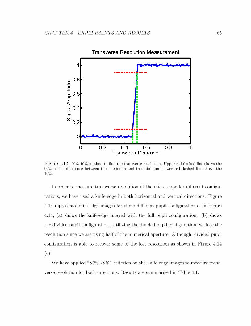
CHAPTER 4. EXPERIMENTS AND RESULTS 65
Figure 4.12: 90%-10% method to find the transverse resolution. Upper red dashed line shows the90% of the difference between the maximum and the minimum; lower red dashed line shows the10%.
In order to measure transverse resolution of the microscope for different configu-
rations, we have used a knife-edge in both horizontal and vertical directions. Figure
4.14 represents knife-edge images for three different pupil configurations. In Figure
4.14, (a) shows the knife-edge imaged with the full pupil configuration. (b) shows
the divided pupil configuration. Utilizing the divided pupil configuration, we lose the
resolution since we are using half of the numerical aperture. Although, divided pupil
configuration is able to recover some of the lost resolution as shown in Figure 4.14
(c).
We have applied ”90%-10% ” criterion on the knife-edge images to measure trans-
verse resolution for both directions. Results are summarized in Table 4.1.

CHAPTER 4. EXPERIMENTS AND RESULTS 66
Axial Resolution Measurement
To measure axial resolution, we have used a nano-mover to move the sample in the
axial direction. We have used a mirror as sample and measure the power of the de-
tected light. Therefore, when the sample is in focus, we measure the highest detected
power, and as we move the mirror out of focus, we will lose power. Distribution of
power versus axial distance from focus will show the axial resolution. Figure 4.15
shows the power distribution versus axial distance from the focus for three different
pupil configurations.
Figure 4.13: Measurement of the axial resolution. The axial distance between two green dashedlines is defined as axial resolution.

CHAPTER 4. EXPERIMENTS AND RESULTS 67
4.2.3 Results
Results are summarized in Table 4.1. As we expected, the full pupil configuration has
the best transverse resolution and the divided pupil is next, and we expected that
the half pupil configuration to be the worst and results, confirms our expectations.
Figure 4.14: Knife-edge images for three different pupil configurations. a. divided pupil config-uration, b. half pupil configuration and c. full pupil configuration. Small part of each image ismagnified to show the transition from completely reflecting(bright) to completely transparent(dark)surfaces. Faster transition indicates better resolution. Fluctuations are result of synchronizationsignals in the data acquisition which happens in the direction of orthogonal to scanning direction.
Configuration Lateral(V) Lateral(H) Axial Pixel size Sampling distanceFull Pupil 0.5 µm 1 µm 1.75 µm 130 nm 157 nmHalf Pupil 1.1 µm 1.7 µm 4.62 µm 130 nm 157 nm
Divided Pupil 0.8 µm 1.7 µm 2.37 µm 130 nm 157 nm
Table 4.1: Summary of the resolution measurement. Pixel size is the size of each individual pixelon the sample. Sampling distance corresponds to scanning distance on the sample.
In our next step, we were able to image a business card. The image is presented
in Figure 4.16.

CHAPTER 4. EXPERIMENTS AND RESULTS 68
Figure 4.15: Axial scan for three different pupil configurations. Full pupil has a higher valueat the peak, because using the full pupil for illumination; more power is delivered to the sample.In half pupil configurations, we lose sectioning ability as plot is flattened. Utilizing divided pupilconfiguration will recover some of the loss of sectioning ability.
4.3 High Brightness LED as Light Source
As discussed in previous chapters, in order to obtain an image in confocal microscopy
a high radiance light source is required. Usually lasers provide such radiance, but
our goal in this project was to examine the performance of recently developed high
brightness LED as the light source. The LED was kindly provided by our collaborators
at (Suzhou Institute of Biomedical Engineering and Technology Chinese Academy of
Sciences, Suzhou, China). Since the LED does not have spec sheet, the first step of
the project was to find basic specifications of the LED.
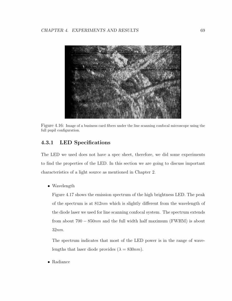
CHAPTER 4. EXPERIMENTS AND RESULTS 69
Figure 4.16: Image of a business card fibers under the line scanning confocal microscope using thefull pupil configuration.
4.3.1 LED Specifications
The LED we used does not have a spec sheet, therefore, we did some experiments
to find the properties of the LED. In this section we are going to discuss important
characteristics of a light source as mentioned in Chapter 2.
• Wavelength
Figure 4.17 shows the emission spectrum of the high brightness LED. The peak
of the spectrum is at 812nm which is slightly different from the wavelength of
the diode laser we used for line scanning confocal system. The spectrum extends
from about 700 − 850nm and the full width half maximum (FWHM) is about
32nm.
The spectrum indicates that most of the LED power is in the range of wave-
lengths that laser diode provides (λ = 830nm).
• Radiance

CHAPTER 4. EXPERIMENTS AND RESULTS 70
Figure 4.17: Emission spectrum of the high brightness LED. Red dashed lines indicate FWHM ofthe spectrum. The maximum emission occurs at 812nm and the FWHM is about 32nm.
As discussed in Chapter 2, radiance of a light source is defined as the amount
of light the source provides in a unit of time, area and solid angle (Figure 4.18).
Therefore, the radiance of the LED is calculated, based on the total optical
power measured in front of the LED and the area of LED.
The area of the LED is measured to be around 1mm2. Also the power is
measured to be 30mW . Assuming uniformity and the solid angle Ω = 2π, the
half space that LED is radiating the light. The radiance of the LED is calculated
as in Equation 4.1.

CHAPTER 4. EXPERIMENTS AND RESULTS 71
Figure 4.18: Geometry of area and solid angle for the source and the detector.
L =Φ
AΩ(4.1)
Therefore, the radiance of the LED is calculated to be around 4.77×10³Watts/m2/sr.
To compare the radiance of the LED with the radiance of the laser diode of the
previous setup, the same calculation for the laser diode has been done. As dis-
cussed before, the radiance of a laser is calculated as in Equation 2.7. The total
power of the laser diode is measured to be 24mW . Therefore, the laser radiance
is 3.48× 10¹⁰Watts/m2/sr.
As the calculations show, the laser diode provides higher radiance for the con-
focal microscope. Low radiance is the most important problem of the LEDs
and the main reason that LEDs have never been used as the light source for a
confocal microscope.
4.3.2 Design
In the new design, the laser and the cylindrical lens have been removed from the setup
and a high brightness LED with the peak wavelength about 850nm and a slit are used.
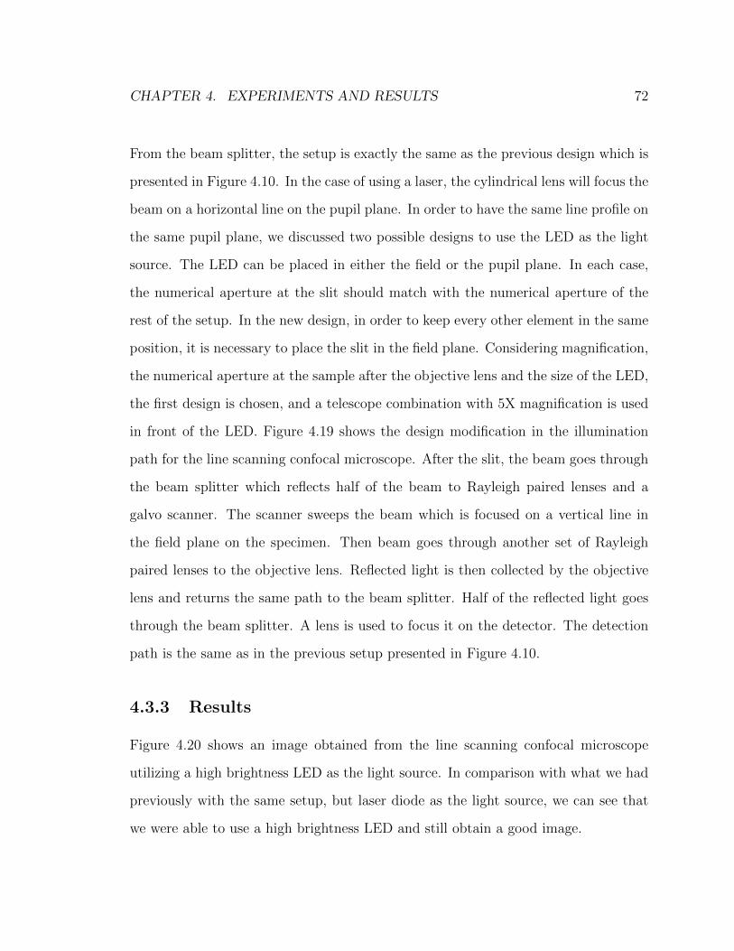
CHAPTER 4. EXPERIMENTS AND RESULTS 72
From the beam splitter, the setup is exactly the same as the previous design which is
presented in Figure 4.10. In the case of using a laser, the cylindrical lens will focus the
beam on a horizontal line on the pupil plane. In order to have the same line profile on
the same pupil plane, we discussed two possible designs to use the LED as the light
source. The LED can be placed in either the field or the pupil plane. In each case,
the numerical aperture at the slit should match with the numerical aperture of the
rest of the setup. In the new design, in order to keep every other element in the same
position, it is necessary to place the slit in the field plane. Considering magnification,
the numerical aperture at the sample after the objective lens and the size of the LED,
the first design is chosen, and a telescope combination with 5X magnification is used
in front of the LED. Figure 4.19 shows the design modification in the illumination
path for the line scanning confocal microscope. After the slit, the beam goes through
the beam splitter which reflects half of the beam to Rayleigh paired lenses and a
galvo scanner. The scanner sweeps the beam which is focused on a vertical line in
the field plane on the specimen. Then beam goes through another set of Rayleigh
paired lenses to the objective lens. Reflected light is then collected by the objective
lens and returns the same path to the beam splitter. Half of the reflected light goes
through the beam splitter. A lens is used to focus it on the detector. The detection
path is the same as in the previous setup presented in Figure 4.10.
4.3.3 Results
Figure 4.20 shows an image obtained from the line scanning confocal microscope
utilizing a high brightness LED as the light source. In comparison with what we had
previously with the same setup, but laser diode as the light source, we can see that
we were able to use a high brightness LED and still obtain a good image.

CHAPTER 4. EXPERIMENTS AND RESULTS 73
Figure 4.19: Line-scanning confocal microscope design. a) Illumination path to sample. b)Detection path from the sample to the detector. c) First design option to place LED in the fieldplane. d) Second design option is to place LED in pupil plane.
Measuring the optical power after the slit and considering 4% specular reflection
loss from each surface, plus 50% loss at the beam splitter, the estimated amount
of power reaches the detector is about 2.18mW . In comparison, our laser diode can
provide 25mW which about 4.1mW of it reaches the detector. We were able to obtain
an image with a 1-D CMOS linear array detector. We applied 90%-10% criterion [3]
on the knife-edge images to measure the transverse resolution for both directions.
Figure 4.21 shows the image of the horizontal knife-edge with the corresponding plot
for the pixel values. The response for each scanned line is assumed to be the same in
the horizontal direction, therefore; the plotted signal is the average over all the 640
horizontal lines.
Figure 4.22 represents the image of the vertical knife-edge and the corresponding
plot for the pixel values. Again, the response for each scanned line is assumed to be
the same in the vertical direction. The plotted signal is the average over the 1024
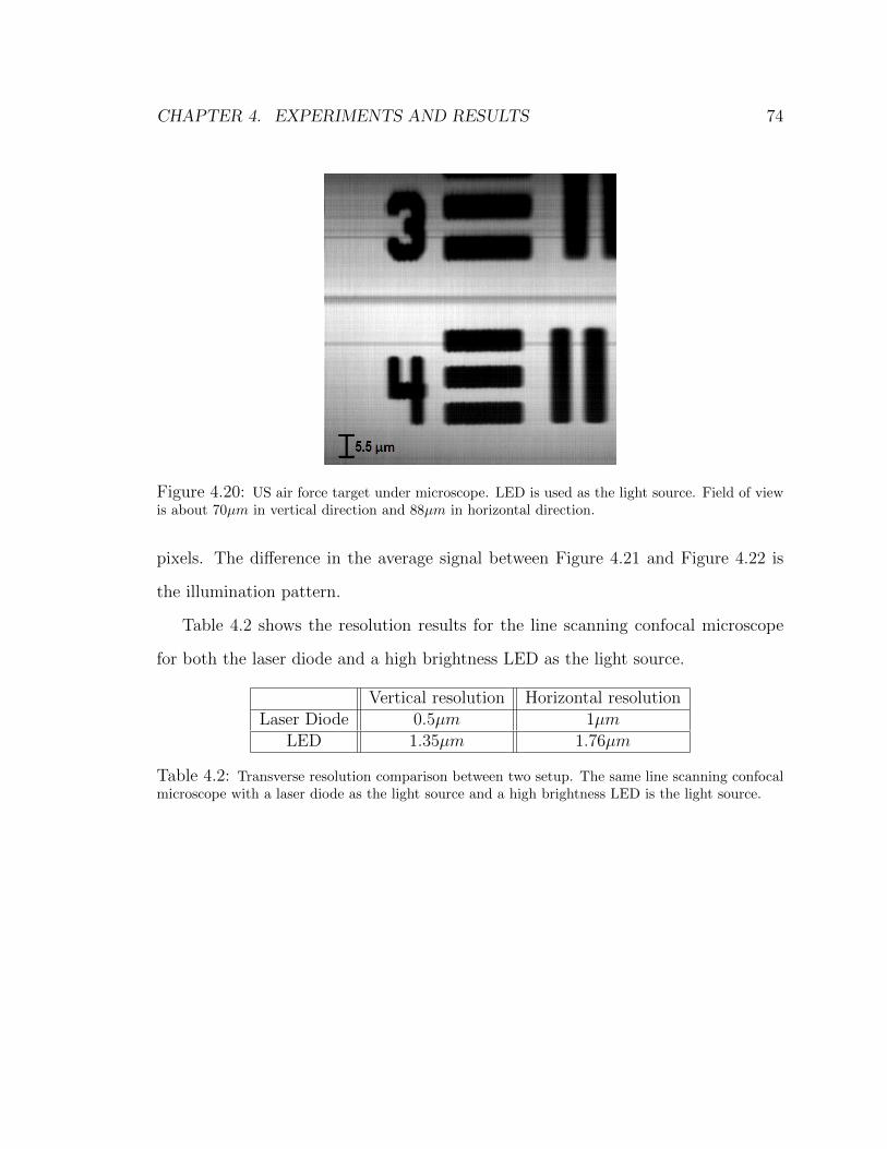
CHAPTER 4. EXPERIMENTS AND RESULTS 74
Figure 4.20: US air force target under microscope. LED is used as the light source. Field of viewis about 70µm in vertical direction and 88µm in horizontal direction.
pixels. The difference in the average signal between Figure 4.21 and Figure 4.22 is
the illumination pattern.
Table 4.2 shows the resolution results for the line scanning confocal microscope
for both the laser diode and a high brightness LED as the light source.
Vertical resolution Horizontal resolutionLaser Diode 0.5µm 1µm
LED 1.35µm 1.76µm
Table 4.2: Transverse resolution comparison between two setup. The same line scanning confocalmicroscope with a laser diode as the light source and a high brightness LED is the light source.

CHAPTER 4. EXPERIMENTS AND RESULTS 75
Figure 4.21: Image of the horizontal knife-edge with the corresponding averaged detected signalfrom the detector. The 90%-10% criterion is applied on the signal, to measure the resolution. Theresolution is defined as the transverse distance between the corresponding spots detected by thegreen dashed lines..
Figure 4.22: Image of the vertical knife-edge with the corresponding averaged detected signalfrom the detector. The 90%-10% criterion is applied on the signal, to measure the resolution. Theresolution is defined as the transverse distance between the corresponding spots detected by thegreen dashed lines.
Chapter 5
Conclusion
In this document we have discussed confocal microscopy, specifically reflectance con-
focal microscopy. In Chapter 1 basic concepts of microscopy were discussed. We
started from Ernst Abbe’s equation and definition of the numerical aperture of an
optical system. We discussed the relation between lateral resolution with the working
numerical aperture of an optical microscope. As one of the most important part a
confocal microscope, the pinhole and its functionality was reviewed. Since our re-
search was mainly concentrated on line scanning reflectance confocal microscope, at
the end of Chapter 1 we discussed slit aperture along with pinhole aperture and also
line array detectors.
Chapter 4 discussed experiments and results of our research. Starting with point
scanning confocal microscope with dual wedge scanning system. The distinct feature
of the point scanning is the scanning system which utilizes two rotating prisms to scan
the field of view. We have added fluorescence mode to the existed reflectance confocal
microscope. The confocal microscope with two imaging modalities was used to image
pure melanin and melanin in human hair. Results are published in International
76

CHAPTER 5. CONCLUSION 77
Society for Optics and Photonics [31].
Next set of our work was done on line scanning confocal microscope. We have
worked on different pupil configurations as discussed in Chapter 3. Results show that
transition from the full pupil configuration to the half pupil configuration, we lose
resolution as expected. In the half pupil configuration, we use half of the numeri-
cal aperture which results in losing transverse and axial resolution by factor of two
and four, respectively. Utilizing the divided pupil configuration, results in recovering
the lost resolution. The divided pupil configuration uses only half of the numerical
aperture like the half pupil configuration, but it utilizes one half for illumination and
the other half for detection. We realized that although divided pupil configuration is
not as good as full pupil configuration in terms of resolution, but the divided pupil
configuration is more successful in rejecting unwanted multiply scattered photons.
Therefore, we can recover some of the lost resolution utilizing divided pupil configu-
ration.
As discussed in Chapter 4 one of our research goals was to use a high brightness
LED instead of a laser light source. Therefore, Chapter 2 reviewed characteristics of
a light source. We began the discussion by general properties of a light source such
as radiance, wavelength and coherence. Radiance is the most important property
of a light source specially in confocal microscopy since it is required to deliver high
radiance to the specimen. As the most common group of light sources being used in
confocal microscopy, Chapter 2 discussed lasers and their properties. In our research
we have used a diode laser as the light source. One part of our research was focused
on non-laser light sources since we used a high brightness LED as the light source
later in our project. The third set of experiments on confocal microscopy, we have
replaced the laser light source with a recently developed high brightness LED that

CHAPTER 5. CONCLUSION 78
provides enough radiance for confocal reflectance imaging. This was the first time
that an LED is used as the light source of a confocal microscope. Unlike lasers, LEDs
are incoherent light sources. Therefore, images provided with high brightness LED
is speckle free. Also, high brightness LED is much cheaper and easier to work with
in comparison the laser diode. Results are published at 2014 40th Annual Northeast
Bioengineering Conference (NEBEC) Proceedings.
To summarize, we have discussed physics behind confocal microscopy, its limita-
tions and advantages. We have done experiment on both point scanning and line
scanning confocal microscopes, in both reflectance and fluorescence modalities. We
have discussed different pupil configurations and two different light source for the line
scanning confocal microscope and provide analysis of the resolution for each imaging
system.

Chapter 6
Future Work
With all discussion about confocal microscopy and experiments, there is still a lot
more to do in the future. Main tasks and ideas for future work are presented in this
chapter.
6.1 Quantify Multiply Scattered Photons Rejec-
tion
We discussed in Chapter 4 that full pupil configuration is poor because it utilizes
the full numerical aperture. We also showed in experiments that divided pupil is
more successful in rejecting more of multiply scattered photons, but we could not
quantify this. One idea to quantify the ability of each configuration to reject multiply
scattered photons, is to calculate Laplacian of the image for the same field of view
but in different pupil configurations. Figure 6.1 shows weight function for each cell
with its 8 neighbor cells. Close neighbors has higher weight since there is a direct
correlation between close neighbors.
79

CHAPTER 6. FUTURE WORK 80
Figure 6.1: Weights for applying Laplacian transform. The center pixel has the weight of 20, itsclose neighbors has -4 and far neighbors has -1.
This is basically the same as applying a high-pass filter to the image. It is a
fairly good assumption that unwanted multiply scattered photons contribute to the
image uniformly. Ideally, if there is no unwanted photons contributed in the image,
resulting image after applying the Laplacian transform, would be zero except for
pixels correspond to knife-edge. Therefore, the more unwanted photons leaked into
the detector, the higher the value of the elements in the resulting image after applying
Laplacian transform.
6.2 Image Larger Area with Dual-Line Scanning
We have discussed the line scanning system. Also we mentioned that a high brightness
LED can provide good resolution. The fact that an LED can replace the laser in
confocal scanning system, gives us the chance to build instruments with less cost,
since LEDs are much cheaper than lasers, which is important specially in clinical

CHAPTER 6. FUTURE WORK 81
instrumentation.
The idea of dual-line scanning system consists of two main parts. First, creating
two lines on the sample at the same time, which is easily possible by using a double
slit instead of one. Second, computing the correlation between two scanned lines to
find the scanning direction. Therefore, we can build a probe with dual-line scanning.
While the user is moving the probe on the specimen (like human skin), the first line
scans the specimen and captures the image of a line, the second line is used to register
the first line in the larger field of view to be scanned. Figure 6.2 shows how the idea
of the dual-line scanning probe.
Figure 6.2: Dual-line scanning probe. Blue arrows shows the direction of scanning the probe onthe large field of view. Paired green and red dotted lines are used together to form and register theimage.
As illustrated in Figure 6.2, user scans the probe on the large field of view to be
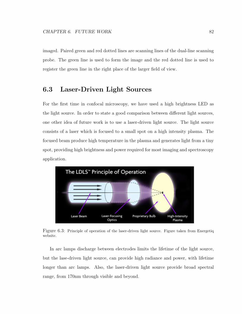
CHAPTER 6. FUTURE WORK 82
imaged. Paired green and red dotted lines are scanning lines of the dual-line scanning
probe. The green line is used to form the image and the red dotted line is used to
register the green line in the right place of the larger field of view.
6.3 Laser-Driven Light Sources
For the first time in confocal microscopy, we have used a high brightness LED as
the light source. In order to state a good comparison between different light sources,
one other idea of future work is to use a laser-driven light source. The light source
consists of a laser which is focused to a small spot on a high intensity plasma. The
focused beam produce high temperature in the plasma and generates light from a tiny
spot, providing high brightness and power required for most imaging and spectroscopy
application.
Figure 6.3: Principle of operation of the laser-driven light source. Figure taken from Energetiqwebsite.
In arc lamps discharge between electrodes limits the lifetime of the light source,
but the lase-driven light source, can provide high radiance and power, with lifetime
longer than arc lamps. Also, the laser-driven light source provide broad spectral
range, from 170nm through visible and beyond.

Bibliography
[1] N. S. Claxton, T. J. Fellers, and M. W. Davidson, “Laser scanning confocal
microscopy,” Department of Optical Microscopy and Digital Imaging, National
High Magnetic Field Laboratory, The Florida State University, 2006.
[2] Y. G. Patel, M. Rajadhyaksha, and C. A. DiMarzio, “Optimization of pupil
design for point-scanning and line-scanning confocal microscopy,” Biomedical
optics express, vol. 2, no. 8, pp. 2231–2242, 2011.
[3] P. J. Dwyer, C. A. DiMarzio, J. M. Zavislan, W. J. Fox, and M. Rajadhyaksha,
“Confocal reflectance theta line scanning microscope for imaging human skin in
vivo,” Optics letters, vol. 31, no. 7, pp. 942–944, 2006.
[4] C. A. DiMarzio, Optics for Engineers. Crc Press, 2011.
[5] J. Pawley, Handbook of biological confocal microscopy. Springer, 2010.
[6] W. C. Warger Ii, C. A. DiMarzio, et al., “Dual-wedge scanning confocal re-
flectance microscope,” Optics letters, vol. 32, no. 15, pp. 2140–2142, 2007.
[7] E. Linfoot and E. Wolf, “Phase distribution near focus in an aberration-free
diffraction image,” Proceedings of the Physical Society. Section B, vol. 69, no. 8,
p. 823, 1956.
83

BIBLIOGRAPHY 84
[8] S. J. Wright and D. J. Wright, “Introduction to confocal microscopy,” Cell Bio-
logical Applications of Confocal Microscopy, in Methods in Cell Biology, vol. 70,
pp. 1–85, 2002.
[9] E. H. Stelzer, “Practical limits to resolution in fluorescence light microscopy,”
Imaging neurons. Cold Spring Harbor Press, Cold Spring Harbor, pp. 12–1, 2000.
[10] J. M. Murray, “Confocal microscopy, deconvolution, and structured illumina-
tion methods,” Live Cell ImagingA Laboratory Manual. RD Goldman and DL
Spector, editors. Cold Spring Harbor Laboratory Press, Cold Spring Harbor, NY,
pp. 239–279, 2005.
[11] T. Wilson and A. Carlini, “Three-dimensional imaging in confocal imaging sys-
tems with finite sized detectors,” Journal of Microscopy, vol. 149, no. 1, pp. 51–
66, 1988.
[12] A. Diaspro et al., Confocal and two-photon microscopy: foundations, applica-
tions, and advances, vol. 1. Wiley-Liss New York, 2002.
[13] B. Matsumoto, Cell biological applications of confocal microscopy. Academic
Press, 2003.
[14] M. Muller, Introduction to confocal fluorescence microscopy, vol. 69. SPIE press,
2006.
[15] A. R. Hibbs, Confocal microscopy for biologists. Kluwer Academic/Plenum Pub-
lishers New York, 2004.
[16] D. B. Murphy and M. W. Davidson, Fundamentals of light microscopy and elec-
tronic imaging. John Wiley & Sons, 2012.

BIBLIOGRAPHY 85
[17] R. H. Webb, “Confocal optical microscopy,” Reports on Progress in Physics,
vol. 59, no. 3, p. 427, 1996.
[18] K. R. Spring, “Detectors for fluorescence microscopy,” in Methods in cellular
imaging, pp. 40–52, Springer, 2001.
[19] R. Anderson and J. A. Parrish, “The optics of human skin.,” Journal of Inves-
tigative Dermatology, vol. 77, no. 1, 1981.
[20] G. Indebetouw and P. Klysubun, “Imaging through scattering media with depth
resolution by use of low-coherence gating in spatiotemporal digital holography,”
Optics Letters, vol. 25, no. 4, pp. 212–214, 2000.
[21] A. K. Fung and H. Eom, “Multiple scattering and depolarization by a ran-
domly rough kirchhoff surface,” Antennas and Propagation, IEEE Transactions
on, vol. 29, no. 3, pp. 463–471, 1981.
[22] R. K. Wang, “Signal degradation by multiple scattering in optical coherence
tomography of dense tissue: a monte carlo study towards optical clearing of
biotissues,” Physics in medicine and biology, vol. 47, no. 13, p. 2281, 2002.
[23] C. J. Koester, “Scanning mirror microscope with optical sectioning characteris-
tics: applications in ophthalmology,” Applied Optics, vol. 19, no. 11, pp. 1749–
1757, 1980.
[24] C. J. Koester, “High efficiency optical sectioning with confocal slits,” Trans. R.
Microsc. Soc, vol. 1, pp. 327–332, 1990.

BIBLIOGRAPHY 86
[25] C. J. Sheppard, W. Gong, and K. Si, “The divided aperture technique for mi-
croscopy through scattering media,” Optics express, vol. 16, no. 21, pp. 17031–
17038, 2008.
[26] P. J. Dwyer, C. A. DiMarzio, and M. Rajadhyaksha, “Confocal theta line-
scanning microscope for imaging human tissues,” Applied optics, vol. 46, no. 10,
pp. 1843–1851, 2007.
[27] D. S. Gareau, S. Abeytunge, and M. Rajadhyaksha, “Line-scanning reflectance
confocal microscopy of human skin: comparison of full-pupil and divided-pupil
configurations,” Optics letters, vol. 34, no. 20, pp. 3235–3237, 2009.
[28] S. Cotton, E. Claridge, and P. Hall, “A skin imaging method based on a colour
formation model and its application to the diagnosis of pigmented skin lesions,”
in Proceedings of Medical Image Understanding and Analysis, vol. 99, pp. 49–52,
Citeseer, 1999.
[29] J. D. Whited and J. M. Grichnik, “Does this patient have a mole or a
melanoma?,” Jama, vol. 279, no. 9, pp. 696–701, 1998.
[30] J. Kerimo, M. Rajadhyaksha, and C. A. DiMarzio, “Enhanced eumelanin emis-
sion by stepwise three-photon excitation,” in SPIE BiOS, pp. 79031X–79031X,
International Society for Optics and Photonics, 2011.
[31] Y. Mega, J. Kerimo, J. P. Robinson, A. Vakili, N. Johnson, and C. DiMarzio,
“Three-photon fluorescence imaging of melanin with a dual-wedge confocal scan-
ning system,” in SPIE BiOS, pp. 822637–822637, International Society for Optics
and Photonics, 2012.