Computational Harmonic Analysis meets Imaging Sciences · PDF fileComputational Harmonic...
92
Computational Harmonic Analysis meets Imaging Sciences Part II Gitta Kutyniok (Technische Universit¨ at Berlin) BMS Summer School Berlin, July 25 – August 5, 2016 Gitta Kutyniok (TU Berlin) Computational Harmonic Analysis BMS Summer School’16 1 / 64
Transcript of Computational Harmonic Analysis meets Imaging Sciences · PDF fileComputational Harmonic...
Computational Harmonic Analysis meetsImaging Sciences
Part II
Gitta Kutyniok(Technische Universitat Berlin)
BMS Summer SchoolBerlin, July 25 – August 5, 2016
Gitta Kutyniok (TU Berlin) Computational Harmonic Analysis BMS Summer School’16 1 / 64
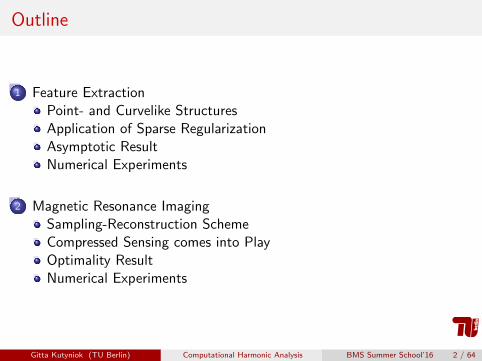
Outline
1 Feature ExtractionPoint- and Curvelike StructuresApplication of Sparse RegularizationAsymptotic ResultNumerical Experiments
2 Magnetic Resonance ImagingSampling-Reconstruction SchemeCompressed Sensing comes into PlayOptimality ResultNumerical Experiments
Gitta Kutyniok (TU Berlin) Computational Harmonic Analysis BMS Summer School’16 2 / 64

We start with Feature Extraction!
Gitta Kutyniok (TU Berlin) Computational Harmonic Analysis BMS Summer School’16 3 / 64
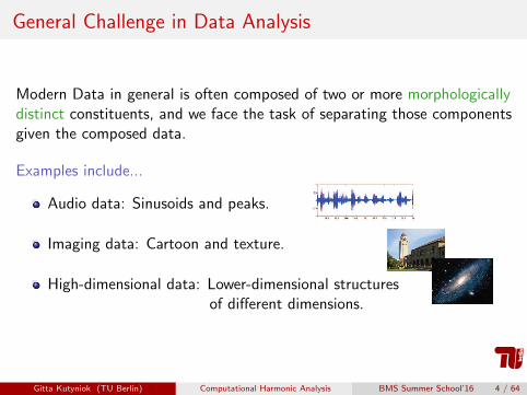
General Challenge in Data Analysis
Modern Data in general is often composed of two or more morphologicallydistinct constituents, and we face the task of separating those componentsgiven the composed data.
Examples include...
Audio data: Sinusoids and peaks.
Imaging data: Cartoon and texture.
High-dimensional data: Lower-dimensional structuresof different dimensions.
Gitta Kutyniok (TU Berlin) Computational Harmonic Analysis BMS Summer School’16 4 / 64
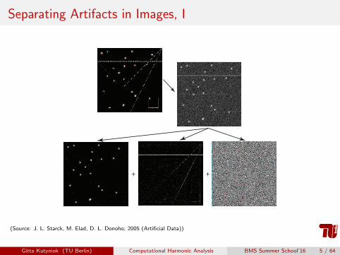
Separating Artifacts in Images, I
+ +
(Source: J. L. Starck, M. Elad, D. L. Donoho; 2005 (Artificial Data))
Gitta Kutyniok (TU Berlin) Computational Harmonic Analysis BMS Summer School’16 5 / 64
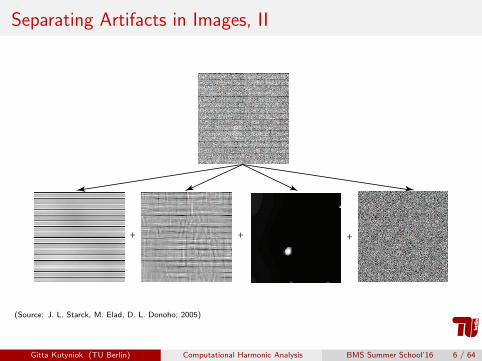
Separating Artifacts in Images, II
+ + +
(Source: J. L. Starck, M. Elad, D. L. Donoho; 2005)
Gitta Kutyniok (TU Berlin) Computational Harmonic Analysis BMS Summer School’16 6 / 64
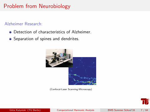
Problem from Neurobiology
Alzheimer Research:
Detection of characteristics of Alzheimer.
Separation of spines and dendrites.
(Confocal-Laser Scanning-Microscopy)
Gitta Kutyniok (TU Berlin) Computational Harmonic Analysis BMS Summer School’16 7 / 64
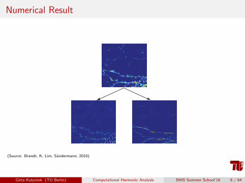
Numerical Result
+
(Source: Brandt, K, Lim, Sundermann; 2010)
Gitta Kutyniok (TU Berlin) Computational Harmonic Analysis BMS Summer School’16 8 / 64

How does Sparse Regularization help
with Component Separation?
Gitta Kutyniok (TU Berlin) Computational Harmonic Analysis BMS Summer School’16 9 / 64
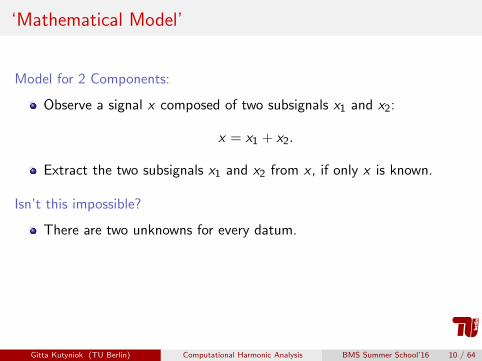
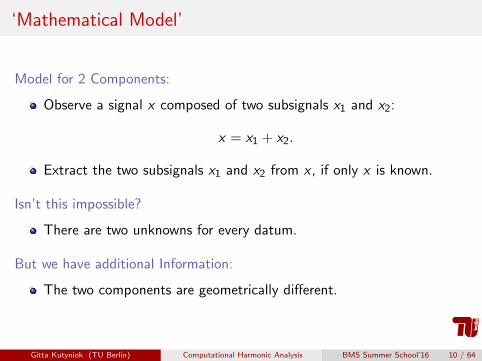
‘Mathematical Model’
Model for 2 Components:
Observe a signal x composed of two subsignals x1 and x2:
x = x1 + x2.
Extract the two subsignals x1 and x2 from x , if only x is known.
Isn’t this impossible?
There are two unknowns for every datum.
But we have additional Information:
The two components are geometrically different.
Gitta Kutyniok (TU Berlin) Computational Harmonic Analysis BMS Summer School’16 10 / 64
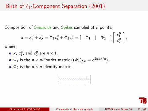
Birth of `1-Component Separation (2001)
Composition of Sinusoids and Spikes sampled at n points:
x = x01 + x0
2 = Φ1c01 + Φ2c
02 = [ Φ1 | Φ2 ]
[c0
1
c02
],
where
x , c01 , and c0
2 are n × 1.
Φ1 is the n × n-Fourier matrix ((Φ1)t,k = e2πitk/n).
Φ2 is the n × n-Identity matrix.
0 50 100 150 200 250-1
-0.5
0
0.5
1
Gitta Kutyniok (TU Berlin) Computational Harmonic Analysis BMS Summer School’16 11 / 64
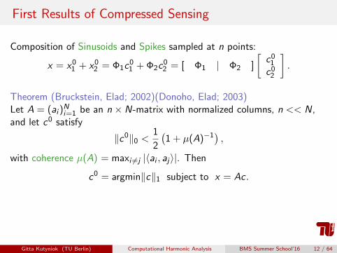
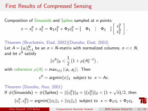
First Results of Compressed Sensing
Composition of Sinusoids and Spikes sampled at n points:
x = x01 + x0
2 = Φ1c01 + Φ2c
02 = [ Φ1 | Φ2 ]
[c0
1
c02
].
Theorem (Bruckstein, Elad; 2002)(Donoho, Elad; 2003)Let A = (ai )
Ni=1 be an n × N-matrix with normalized columns, n << N,
and let c0 satisfy
‖c0‖0 <1
2
(1 + µ(A)−1
),
with coherence µ(A) = maxi 6=j |〈ai , aj〉|. Then
c0 = argmin‖c‖1 subject to x = Ac .
Theorem (Donoho, Huo; 2001)If #(Sinusoids) + #(Spikes) = ‖(c0
1 )‖0 + ‖(c02 )‖0 < (1 +
√n)/2, then
(c01 , c
02 ) = argmin(‖c1‖1 + ‖c2‖1) subject to x = Φ1c1 + Φ2c2.
Gitta Kutyniok (TU Berlin) Computational Harmonic Analysis BMS Summer School’16 12 / 64
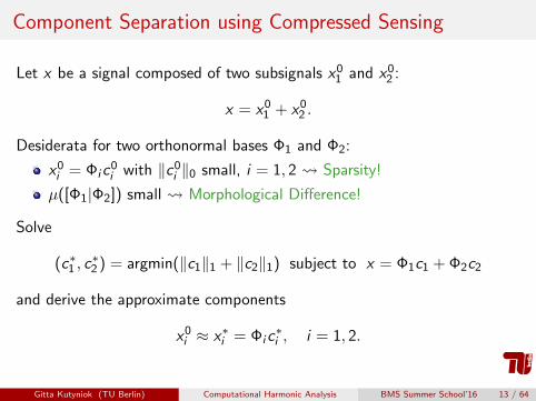
Component Separation using Compressed Sensing
Let x be a signal composed of two subsignals x01 and x0
2 :
x = x01 + x0
2 .
Desiderata for two orthonormal bases Φ1 and Φ2:
x0i = Φic
0i with ‖c0
i ‖0 small, i = 1, 2 Sparsity!
µ([Φ1|Φ2]) small Morphological Difference!
Solve
(c∗1 , c∗2 ) = argmin(‖c1‖1 + ‖c2‖1) subject to x = Φ1c1 + Φ2c2
and derive the approximate components
x0i ≈ x∗i = Φic
∗i , i = 1, 2.
Gitta Kutyniok (TU Berlin) Computational Harmonic Analysis BMS Summer School’16 13 / 64
Two Paths
Gitta Kutyniok (TU Berlin) Computational Harmonic Analysis BMS Summer School’16 14 / 64
Avalanche of Recent Work
Problem: Solve x = Ac0 with A an n × N-matrix (n < N).
Deterministic World:
Mutual coherence of A = (ak)k .
Bound ‖c0‖0 dependent on µ(A).
Efficiently solve the problem x = Ac0.
Contributors: Bruckstein, Cohen, Dahmen, DeVore, Donoho, Elad,Fuchs, Gribonval, Huo, K, Rauhut, Temlyakov, Tropp, ...
Random World:
Restricted isometry constants of a random A = (ak)k .
Bound ‖c0‖0 by n/(2 log(N/n))(1 + o(1)).
Efficiently solve the problem x = Ac0 with high probability.
Contributors: Candes, Donoho, Fornasier, K, Krahmer, Rauhut,Romberg, Tanner, Tao, Tropp, Vershynin, Ward, ...
Gitta Kutyniok (TU Berlin) Computational Harmonic Analysis BMS Summer School’16 15 / 64
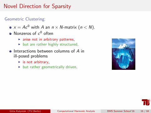
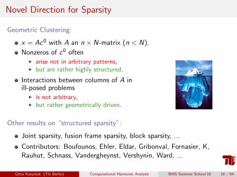
Novel Direction for Sparsity
Geometric Clustering:
x = Ac0 with A an n × N-matrix (n < N).
Nonzeros of c0 oftenI arise not in arbitrary patterns,I but are rather highly structured.
Interactions between columns of A inill-posed problems
I is not arbitrary,I but rather geometrically driven.
Other results on “structured sparsity”:
Joint sparsity, fusion frame sparsity, block sparsity, ...
Contributors: Boufounos, Ehler, Eldar, Gribonval, Fornasier, K,Rauhut, Schnass, Vandergheynst, Vershynin, Ward, ...
Gitta Kutyniok (TU Berlin) Computational Harmonic Analysis BMS Summer School’16 16 / 64

How can these Ideas be applied to
Separation of Points and Curves?
Gitta Kutyniok (TU Berlin) Computational Harmonic Analysis BMS Summer School’16 17 / 64
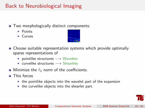
Back to Neurobiological Imaging
Two morphologically distinct components:I PointsI Curves
Choose suitable representation systems which provide optimallysparse representations of
I pointlike structures −→ WaveletsI curvelike structures −→ Shearlets
Minimize the `1 norm of the coefficients.
This forcesI the pointlike objects into the wavelet part of the expansionI the curvelike objects into the shearlet part.
Gitta Kutyniok (TU Berlin) Computational Harmonic Analysis BMS Summer School’16 18 / 64
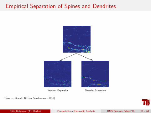
Empirical Separation of Spines and Dendrites
+
Wavelet Expansion Shearlet Expansion
(Source: Brandt, K, Lim, Sundermann; 2010)
Gitta Kutyniok (TU Berlin) Computational Harmonic Analysis BMS Summer School’16 19 / 64
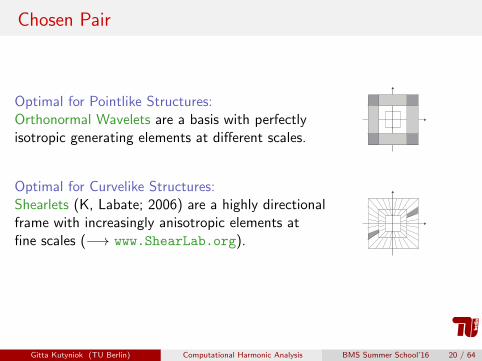
Chosen Pair
Optimal for Pointlike Structures:Orthonormal Wavelets are a basis with perfectlyisotropic generating elements at different scales.
Optimal for Curvelike Structures:Shearlets (K, Labate; 2006) are a highly directionalframe with increasingly anisotropic elements atfine scales (−→ www.ShearLab.org).
Gitta Kutyniok (TU Berlin) Computational Harmonic Analysis BMS Summer School’16 20 / 64
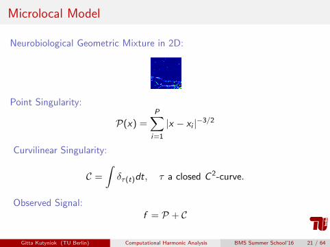
Microlocal Model
Neurobiological Geometric Mixture in 2D:
Point Singularity:
P(x) =P∑i=1
|x − xi |−3/2
Curvilinear Singularity:
C =
∫δτ(t)dt, τ a closed C 2-curve.
Observed Signal:f = P + C
Gitta Kutyniok (TU Berlin) Computational Harmonic Analysis BMS Summer School’16 21 / 64
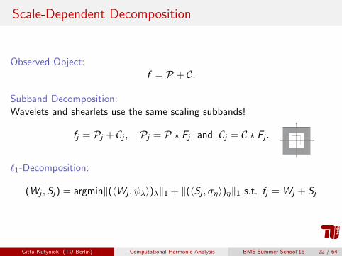
Scale-Dependent Decomposition
Observed Object:f = P + C.
Subband Decomposition:Wavelets and shearlets use the same scaling subbands!
fj = Pj + Cj , Pj = P ? Fj and Cj = C ? Fj .
`1-Decomposition:
(Wj ,Sj) = argmin‖(〈Wj , ψλ〉)λ‖1 + ‖(〈Sj , ση〉)η‖1 s.t. fj = Wj + Sj
Gitta Kutyniok (TU Berlin) Computational Harmonic Analysis BMS Summer School’16 22 / 64
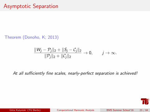
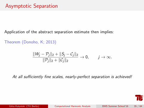
Asymptotic Separation
Theorem (Donoho, K; 2013)
‖Wj − Pj‖2 + ‖Sj − Cj‖2
‖Pj‖2 + ‖Cj‖2→ 0, j →∞.
At all sufficiently fine scales, nearly-perfect separation is achieved!
Gitta Kutyniok (TU Berlin) Computational Harmonic Analysis BMS Summer School’16 23 / 64
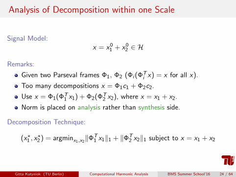
Analysis of Decomposition within one Scale
Signal Model:x = x0
1 + x02 ∈ H
Remarks:
Given two Parseval frames Φ1, Φ2 (Φi (ΦTi x) = x for all x).
Too many decompositions x = Φ1c1 + Φ2c2.
Use x = Φ1(ΦT1 x1) + Φ2(ΦT
2 x2), where x = x1 + x2.
Norm is placed on analysis rather than synthesis side.
Decomposition Technique:
(x?1 , x?2 ) = argminx1,x2
‖ΦT1 x1‖1 + ‖ΦT
2 x2‖1 subject to x = x1 + x2
Gitta Kutyniok (TU Berlin) Computational Harmonic Analysis BMS Summer School’16 24 / 64

Relative Sparsity and Cluster Coherence
Let Φ1 = (ϕ1,i )i∈I1 and Φ2 = (ϕ2,i )i∈I2 .
Definition:
For each i = 1, 2, x0i is relatively sparse in Φi w.r.t. Λi , if
‖1Λc1ΦT
1 x01‖1 + ‖1Λc
2ΦT
2 x02‖1 ≤ δ.
We call Λ1 and Λ2 sets of significant coefficients.
We define cluster coherence for Λ1 by
µc(Λ1) = maxj∈I2
∑i∈Λ1
|〈ϕ1,i , ϕ2,j〉|.
Gitta Kutyniok (TU Berlin) Computational Harmonic Analysis BMS Summer School’16 25 / 64
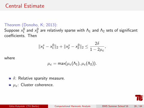
Central Estimate
Theorem (Donoho, K; 2013):Suppose x0
1 and x02 are relatively sparse with Λ1 and Λ2 sets of significant
coefficients. Then
‖x?1 − x01‖2 + ‖x?2 − x0
2‖2 ≤2δ
1− 2µc,
whereµc = max(µc(Λ1), µc(Λ2)).
δ: Relative sparsity measure.
µc : Cluster coherence.
Gitta Kutyniok (TU Berlin) Computational Harmonic Analysis BMS Summer School’16 26 / 64

Application of Previous Result
x : Filtered signal fj (= Pj + Cj).
Φ1: Wavelets filtered with Fj .
Φ2: Shearlets filtered with Fj .
Λ1: Significant wavelet coefficients of 〈ψλ,Pj〉.Λ2: Significant shearlet coefficients of 〈ση, Cj〉.δ: Degree of approximation by significant coefficients.
µc(Λ1), µc(Λ2): Cluster coherence of wavelets-shearlets.
Estimate of error: 2δ1−2µc
.
Gitta Kutyniok (TU Berlin) Computational Harmonic Analysis BMS Summer School’16 27 / 64
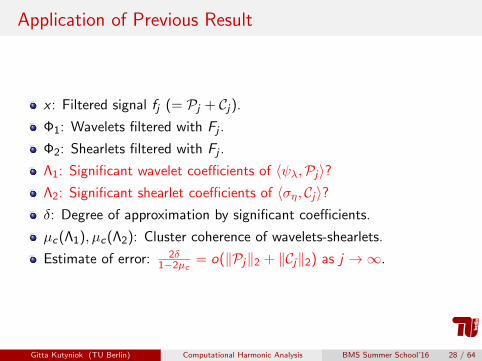
Application of Previous Result
x : Filtered signal fj (= Pj + Cj).
Φ1: Wavelets filtered with Fj .
Φ2: Shearlets filtered with Fj .
Λ1: Significant wavelet coefficients of 〈ψλ,Pj〉?Λ2: Significant shearlet coefficients of 〈ση, Cj〉?δ: Degree of approximation by significant coefficients.
µc(Λ1), µc(Λ2): Cluster coherence of wavelets-shearlets.
Estimate of error: 2δ1−2µc
= o(‖Pj‖2 + ‖Cj‖2) as j →∞.
Gitta Kutyniok (TU Berlin) Computational Harmonic Analysis BMS Summer School’16 28 / 64
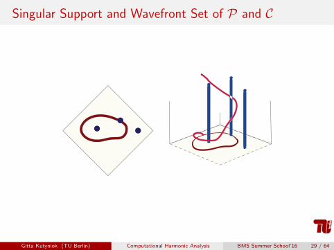
Singular Support and Wavefront Set of P and C
Gitta Kutyniok (TU Berlin) Computational Harmonic Analysis BMS Summer School’16 29 / 64
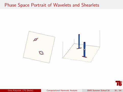
Phase Space Portrait of Wavelets and Shearlets
Gitta Kutyniok (TU Berlin) Computational Harmonic Analysis BMS Summer School’16 30 / 64

Cluster Coherence
Wavelets in Λ1 ≈ vertical tubes clustering around the pointsingularities of P.
Shearlets in Λ2 ≈ tubes clustering around the curvilinear phaseportrait of C.
Single wavelet is incoherent with ensemble of shearlets in Λ2.
Single shearlet is incoherent with ensemble of wavelets in Λ1.
Gitta Kutyniok (TU Berlin) Computational Harmonic Analysis BMS Summer School’16 31 / 64
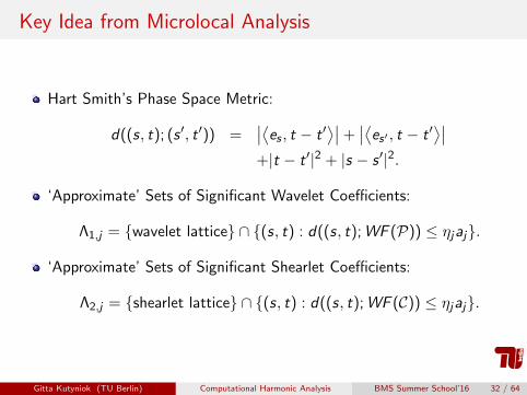
Key Idea from Microlocal Analysis
Hart Smith’s Phase Space Metric:
d((s, t); (s ′, t ′)) =∣∣⟨es , t − t ′
⟩∣∣+∣∣⟨es′ , t − t ′
⟩∣∣+|t − t ′|2 + |s − s ′|2.
‘Approximate’ Sets of Significant Wavelet Coefficients:
Λ1,j = {wavelet lattice} ∩ {(s, t) : d((s, t);WF (P)) ≤ ηjaj}.
‘Approximate’ Sets of Significant Shearlet Coefficients:
Λ2,j = {shearlet lattice} ∩ {(s, t) : d((s, t);WF (C)) ≤ ηjaj}.
Gitta Kutyniok (TU Berlin) Computational Harmonic Analysis BMS Summer School’16 32 / 64
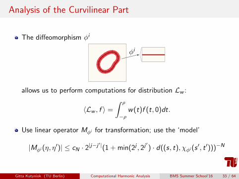
Analysis of the Curvilinear Part
The diffeomorphism φi
φi
allows us to perform computations for distribution Lw :
〈Lw , f 〉 =
∫ ρ
−ρw(t)f (t, 0)dt.
Use linear operator Mφi for transformation; use the ‘model’
|Mφi (η, η′)| ≤ cN · 2|j−j
′|(1 + min(2j , 2j′) · d((s, t), χφi (s
′, t ′)))−N
Gitta Kutyniok (TU Berlin) Computational Harmonic Analysis BMS Summer School’16 33 / 64

Essential Estimates
Proposition:
(Λ1,j) and (Λ2,j) have the following two properties:I asymptotically negligible cluster coherences:
µc(Λ1,j), µc(Λ2,j)→ 0, j →∞.
I asymptotically negligible cluster approximation errors:
δj = δ1,j + δ2,j = o(‖Pj‖2 + ‖Cj‖2), j →∞.
Gitta Kutyniok (TU Berlin) Computational Harmonic Analysis BMS Summer School’16 34 / 64
Asymptotic Separation
Application of the abstract separation estimate then implies:
Theorem (Donoho, K; 2013)
‖Wj − Pj‖2 + ‖Sj − Cj‖2
‖Pj‖2 + ‖Cj‖2→ 0, j →∞.
At all sufficiently fine scales, nearly-perfect separation is achieved!
Gitta Kutyniok (TU Berlin) Computational Harmonic Analysis BMS Summer School’16 35 / 64
Recovery of Fourier Data
or: Fast Data Acquisition in MRI
Gitta Kutyniok (TU Berlin) Computational Harmonic Analysis BMS Summer School’16 36 / 64
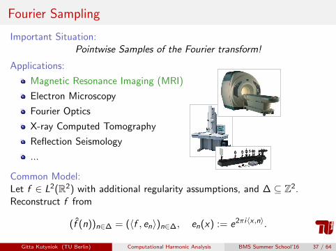
Fourier Sampling
Important Situation:Pointwise Samples of the Fourier transform!
Applications:
Magnetic Resonance Imaging (MRI)
Electron Microscopy
Fourier Optics
X-ray Computed Tomography
Reflection Seismology
...
Common Model:Let f ∈ L2(R2) with additional regularity assumptions, and ∆ ⊆ Z2.Reconstruct f from
(f (n))n∈∆ = (〈f , en〉)n∈∆, en(x) := e2πi〈x ,n〉.
Gitta Kutyniok (TU Berlin) Computational Harmonic Analysis BMS Summer School’16 37 / 64
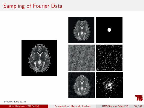
Sampling of Fourier Data
(Source: Lim; 2014)
Gitta Kutyniok (TU Berlin) Computational Harmonic Analysis BMS Summer School’16 38 / 64
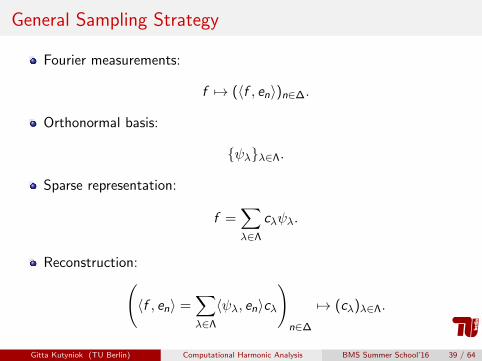
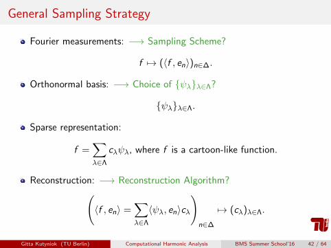
General Sampling Strategy
Fourier measurements: −→ Sampling Scheme?
f 7→ (〈f , en〉)n∈∆.
Orthonormal basis: −→ Choice of {ψλ}λ∈Λ?
{ψλ}λ∈Λ.
Sparse representation: −→ Model for f ?
f =∑λ∈Λ
cλψλ.
Reconstruction: −→ Reconstruction Algorithm?(〈f , en〉 =
∑λ∈Λ
〈ψλ, en〉cλ
)n∈∆
7→ (cλ)λ∈Λ.
Gitta Kutyniok (TU Berlin) Computational Harmonic Analysis BMS Summer School’16 39 / 64
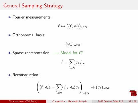
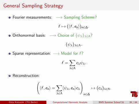

Compressed Sensing Type Approaches
Lustig, Donoho, Pauly; 2007 Sparse MRI: Spirals, L2(R2), Wavelets, `1.
ming‖Ψg‖1 s.t. ‖g |∆ − f |∆‖2 ≤ ε.
Krahmer, Ward; 2014 Variable Density Sampling, CN×N , Haar Wavelets, TV.
Adcock, Hansen, K, Ma; 2014 Block Sampling, L2(R2), Wavelets, Generalized Sampling.
Adcock, Hansen, Poon, Roman; 2014 Multilevel Sampling, H, ONS, `1.
Shi, Yin, Sankaranarayanan, Baraniuk; 2014 Dynamic MRI: Variable Density Sampling, R× Rn, Wavelets, `1.
...
Gitta Kutyniok (TU Berlin) Computational Harmonic Analysis BMS Summer School’16 40 / 64
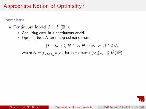
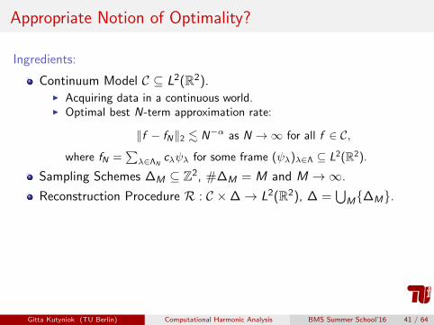
Appropriate Notion of Optimality?
Ingredients:
Continuum Model C ⊆ L2(R2).I Acquiring data in a continuous world.I Optimal best N-term approximation rate:
‖f − fN‖2 . N−α as N →∞ for all f ∈ C,
where fN =∑λ∈ΛN
cλψλ for some frame (ψλ)λ∈Λ ⊆ L2(R2).
Sampling Schemes ∆M ⊆ Z2, #∆M = M and M →∞.
Reconstruction Procedure R : C ×∆→ L2(R2), ∆ =⋃
M{∆M}.
Asymptotic Optimality: We call a sampling-reconstruction scheme(C,∆,R) asymptotically optimal, if, for all f ∈ C,
‖f −R(f ,∆M)‖2 . M−α as M →∞.
Gitta Kutyniok (TU Berlin) Computational Harmonic Analysis BMS Summer School’16 41 / 64

General Sampling Strategy
Fourier measurements: −→ Sampling Scheme?
f 7→ (〈f , en〉)n∈∆.
Orthonormal basis: −→ Choice of {ψλ}λ∈Λ?
{ψλ}λ∈Λ.
Sparse representation: −→ Model for f ?
f =∑λ∈Λ
cλψλ.
Reconstruction: −→ Reconstruction Algorithm?(〈f , en〉 =
∑λ∈Λ
〈ψλ, en〉cλ
)n∈∆
7→ (cλ)λ∈Λ.
Gitta Kutyniok (TU Berlin) Computational Harmonic Analysis BMS Summer School’16 42 / 64
General Sampling Strategy
Fourier measurements: −→ Sampling Scheme?
f 7→ (〈f , en〉)n∈∆.
Orthonormal basis: −→ Choice of {ψλ}λ∈Λ?
{ψλ}λ∈Λ.
Sparse representation:
f =∑λ∈Λ
cλψλ, where f is a cartoon-like function.
Reconstruction: −→ Reconstruction Algorithm?(〈f , en〉 =
∑λ∈Λ
〈ψλ, en〉cλ
)n∈∆
7→ (cλ)λ∈Λ.
Gitta Kutyniok (TU Berlin) Computational Harmonic Analysis BMS Summer School’16 42 / 64
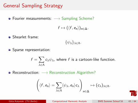
General Sampling Strategy
Fourier measurements: −→ Sampling Scheme?
f 7→ (〈f , en〉)n∈∆.
Shearlet frame:{ψλ}λ∈Λ.
Sparse representation:
f =∑λ∈Λ
cλψλ, where f is a cartoon-like function.
Reconstruction: −→ Reconstruction Algorithm?(〈f , en〉 =
∑λ∈Λ
〈ψλ, en〉cλ
)n∈∆
7→ (cλ)λ∈Λ.
Gitta Kutyniok (TU Berlin) Computational Harmonic Analysis BMS Summer School’16 43 / 64
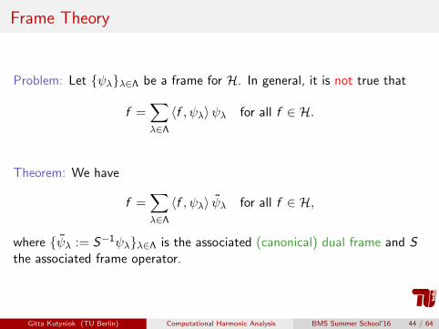
Frame Theory
Problem: Let {ψλ}λ∈Λ be a frame for H. In general, it is not true that
f =∑λ∈Λ
〈f , ψλ〉ψλ for all f ∈ H.
Theorem: We have
f =∑λ∈Λ
〈f , ψλ〉 ψλ for all f ∈ H,
where {ψλ := S−1ψλ}λ∈Λ is the associated (canonical) dual frame and Sthe associated frame operator.
Gitta Kutyniok (TU Berlin) Computational Harmonic Analysis BMS Summer School’16 44 / 64

Problem with Frames
Fourier measurements: −→ Sampling Scheme?
f 7→ (〈f , en〉)n∈∆.
Shearlet frame:{ψλ}λ∈Λ.
Sparse representation:
f =∑λ∈Λ
cλψλ, where f is a cartoon-like function.
Reconstruction: −→ Reconstruction Algorithm?(〈f , en〉 =
∑λ∈Λ
〈ψλ, en〉cλ
)n∈∆
7→ (cλ)λ∈Λ.
Gitta Kutyniok (TU Berlin) Computational Harmonic Analysis BMS Summer School’16 45 / 64
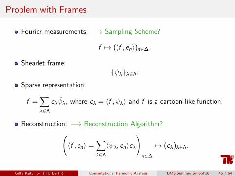
Problem with Frames
Fourier measurements: −→ Sampling Scheme?
f 7→ (〈f , en〉)n∈∆.
Shearlet frame:{ψλ}λ∈Λ.
Sparse representation:
f =∑λ∈Λ
cλψλ, where cλ = 〈f , ψλ〉 and f is a cartoon-like function.
Reconstruction: −→ Reconstruction Algorithm?(〈f , en〉 =
∑λ∈Λ
〈ψλ, en〉cλ
)n∈∆
7→ (cλ)λ∈Λ.
Gitta Kutyniok (TU Berlin) Computational Harmonic Analysis BMS Summer School’16 45 / 64
Dualizable Shearlets...
Gitta Kutyniok (TU Berlin) Computational Harmonic Analysis BMS Summer School’16 46 / 64
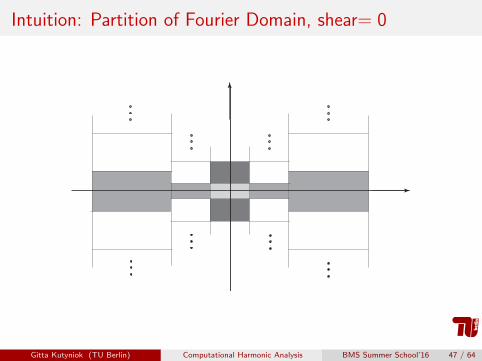
Intuition: Partition of Fourier Domain, shear= 0
Gitta Kutyniok (TU Berlin) Computational Harmonic Analysis BMS Summer School’16 47 / 64
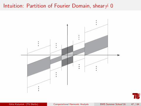
Intuition: Partition of Fourier Domain, shear6= 0
Gitta Kutyniok (TU Berlin) Computational Harmonic Analysis BMS Summer School’16 47 / 64
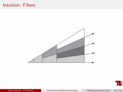
Intuition: Filters
Gitta Kutyniok (TU Berlin) Computational Harmonic Analysis BMS Summer School’16 48 / 64
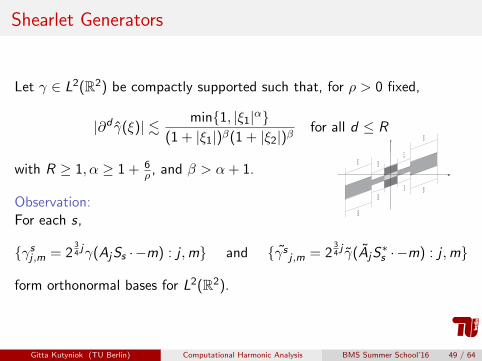
Shearlet Generators
Let γ ∈ L2(R2) be compactly supported such that, for ρ > 0 fixed,
|∂d γ(ξ)| . min{1, |ξ1|α}(1 + |ξ1|)β(1 + |ξ2|)β
for all d ≤ R
with R ≥ 1, α ≥ 1 + 6ρ , and β > α + 1.
Observation:For each s,
{γsj ,m = 234jγ(AjSs ·−m) : j ,m} and {γs j ,m = 2
34j γ(AjS
∗s ·−m) : j ,m}
form orthonormal bases for L2(R2).
Gitta Kutyniok (TU Berlin) Computational Harmonic Analysis BMS Summer School’16 49 / 64
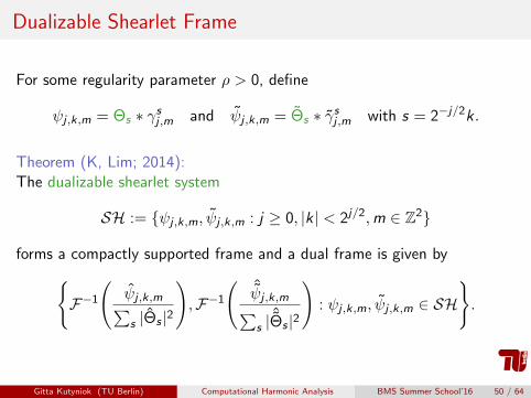
Dualizable Shearlet Frame
For some regularity parameter ρ > 0, define
ψj ,k,m = Θs ∗ γsj ,m and ψj ,k,m = Θs ∗ γsj ,m with s = 2−j/2k .
Theorem (K, Lim; 2014):The dualizable shearlet system
SH := {ψj ,k,m, ψj ,k,m : j ≥ 0, |k| < 2j/2,m ∈ Z2}
forms a compactly supported frame and a dual frame is given by{F−1
(ψj ,k,m∑s |Θs |2
),F−1
(ˆψj ,k,m∑s |
ˆΘs |2
): ψj ,k,m, ψj ,k,m ∈ SH
}.
Gitta Kutyniok (TU Berlin) Computational Harmonic Analysis BMS Summer School’16 50 / 64
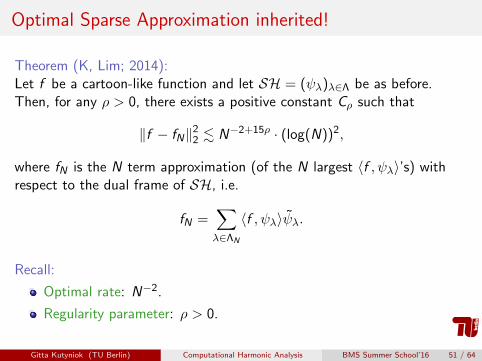
Optimal Sparse Approximation inherited!
Theorem (K, Lim; 2014):Let f be a cartoon-like function and let SH = (ψλ)λ∈Λ be as before.Then, for any ρ > 0, there exists a positive constant Cρ such that
‖f − fN‖22 . N−2+15ρ · (log(N))2,
where fN is the N term approximation (of the N largest 〈f , ψλ〉’s) withrespect to the dual frame of SH, i.e.
fN =∑λ∈ΛN
〈f , ψλ〉ψλ.
Recall:
Optimal rate: N−2.
Regularity parameter: ρ > 0.
Gitta Kutyniok (TU Berlin) Computational Harmonic Analysis BMS Summer School’16 51 / 64
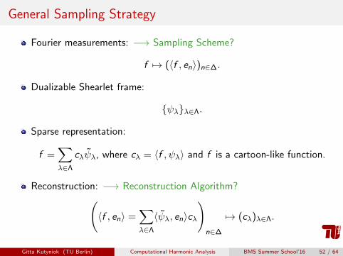
General Sampling Strategy
Fourier measurements: −→ Sampling Scheme?
f 7→ (〈f , en〉)n∈∆.
Dualizable Shearlet frame:
{ψλ}λ∈Λ.
Sparse representation:
f =∑λ∈Λ
cλψλ, where cλ = 〈f , ψλ〉 and f is a cartoon-like function.
Reconstruction: −→ Reconstruction Algorithm?(〈f , en〉 =
∑λ∈Λ
〈ψλ, en〉cλ
)n∈∆
7→ (cλ)λ∈Λ.
Gitta Kutyniok (TU Berlin) Computational Harmonic Analysis BMS Summer School’16 52 / 64

Directional Sampling Strategy
Gitta Kutyniok (TU Berlin) Computational Harmonic Analysis BMS Summer School’16 53 / 64
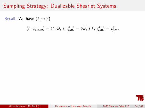
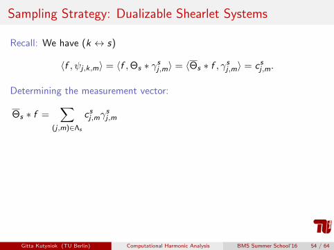
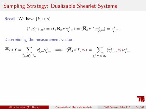
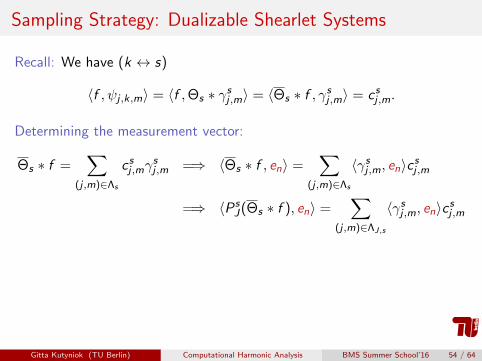
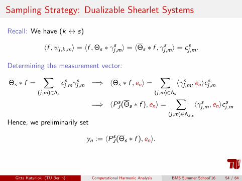
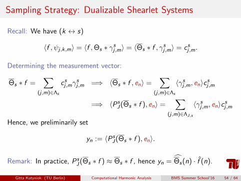
Sampling Strategy: Dualizable Shearlet Systems
Recall: We have (k ↔ s)
〈f , ψj ,k,m〉 = 〈f ,Θs ∗ γsj ,m〉 = 〈Θs ∗ f , γsj ,m〉 = csj ,m.
Determining the measurement vector:
Θs ∗ f =∑
(j ,m)∈Λs
csj ,mγsj ,m =⇒ 〈Θs ∗ f , en〉 =
∑(j ,m)∈Λs
〈γsj ,m, en〉csj ,m
=⇒ 〈PsJ(Θs ∗ f ), en〉 =
∑(j ,m)∈ΛJ,s
〈γsj ,m, en〉csj ,m
Hence, we preliminarily set
yn := 〈PsJ(Θs ∗ f ), en〉.
Remark: In practice, PsJ(Θs ∗ f ) ≈ Θs ∗ f , hence yn = Θs(n) · f (n).
Gitta Kutyniok (TU Berlin) Computational Harmonic Analysis BMS Summer School’16 54 / 64
Sampling Strategy: Dualizable Shearlet Systems
Recall: We have (k ↔ s)
〈f , ψj ,k,m〉 = 〈f ,Θs ∗ γsj ,m〉 = 〈Θs ∗ f , γsj ,m〉 = csj ,m.
Determining the measurement vector:
Θs ∗ f =∑
(j ,m)∈Λs
csj ,mγsj ,m
=⇒ 〈Θs ∗ f , en〉 =∑
(j ,m)∈Λs
〈γsj ,m, en〉csj ,m
=⇒ 〈PsJ(Θs ∗ f ), en〉 =
∑(j ,m)∈ΛJ,s
〈γsj ,m, en〉csj ,m
Hence, we preliminarily set
yn := 〈PsJ(Θs ∗ f ), en〉.
Remark: In practice, PsJ(Θs ∗ f ) ≈ Θs ∗ f , hence yn = Θs(n) · f (n).
Gitta Kutyniok (TU Berlin) Computational Harmonic Analysis BMS Summer School’16 54 / 64
Sampling Strategy: Dualizable Shearlet Systems
Recall: We have (k ↔ s)
〈f , ψj ,k,m〉 = 〈f ,Θs ∗ γsj ,m〉 = 〈Θs ∗ f , γsj ,m〉 = csj ,m.
Determining the measurement vector:
Θs ∗ f =∑
(j ,m)∈Λs
csj ,mγsj ,m =⇒ 〈Θs ∗ f , en〉 =
∑(j ,m)∈Λs
〈γsj ,m, en〉csj ,m
=⇒ 〈PsJ(Θs ∗ f ), en〉 =
∑(j ,m)∈ΛJ,s
〈γsj ,m, en〉csj ,m
Hence, we preliminarily set
yn := 〈PsJ(Θs ∗ f ), en〉.
Remark: In practice, PsJ(Θs ∗ f ) ≈ Θs ∗ f , hence yn = Θs(n) · f (n).
Gitta Kutyniok (TU Berlin) Computational Harmonic Analysis BMS Summer School’16 54 / 64
Sampling Strategy: Dualizable Shearlet Systems
Recall: We have (k ↔ s)
〈f , ψj ,k,m〉 = 〈f ,Θs ∗ γsj ,m〉 = 〈Θs ∗ f , γsj ,m〉 = csj ,m.
Determining the measurement vector:
Θs ∗ f =∑
(j ,m)∈Λs
csj ,mγsj ,m =⇒ 〈Θs ∗ f , en〉 =
∑(j ,m)∈Λs
〈γsj ,m, en〉csj ,m
=⇒ 〈PsJ(Θs ∗ f ), en〉 =
∑(j ,m)∈ΛJ,s
〈γsj ,m, en〉csj ,m
Hence, we preliminarily set
yn := 〈PsJ(Θs ∗ f ), en〉.
Remark: In practice, PsJ(Θs ∗ f ) ≈ Θs ∗ f , hence yn = Θs(n) · f (n).
Gitta Kutyniok (TU Berlin) Computational Harmonic Analysis BMS Summer School’16 54 / 64
General Sampling Scheme
Fourier measurements: −→ Sampling Scheme?
f 7→ (〈f , en〉)n∈∆.
Dualizable Shearlet frame:
{ψλ}λ∈Λ.
Sparse representation:
f =∑λ∈Λ
cλψλ, where cλ = 〈f , ψλ〉 and f is a cartoon-like function.
Reconstruction: −→ Reconstruction Algorithm?(〈f , en〉 =
∑λ∈Λ
〈ψλ, en〉cλ
)n∈∆
7→ (cλ)λ∈Λ.
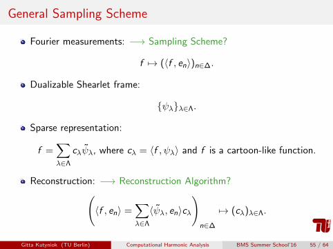
Gitta Kutyniok (TU Berlin) Computational Harmonic Analysis BMS Summer School’16 55 / 64

General Sampling Scheme
Fourier measurements: −→ Sampling Scheme?
f 7→ (〈f , en〉)n∈∆.
Dualizable Shearlet frame:
{ψλ}λ∈Λ.
Sparse representation:
f =∑λ∈Λ
cλψλ, where cλ = 〈f , ψλ〉 and f is a cartoon-like function.
Reconstruction:
(cλ)λ∈Λ = argmin(cλ)λ∈Λ‖(cλ)λ∈Λ‖1 s.t.
(〈f , en〉 =
∑λ∈Λ
〈ψλ, en〉cλ)n∈∆
.
Gitta Kutyniok (TU Berlin) Computational Harmonic Analysis BMS Summer School’16 55 / 64
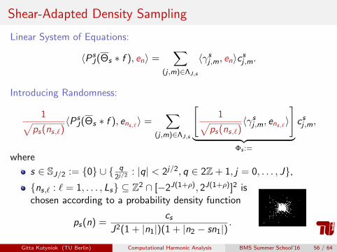
Shear-Adapted Density Sampling
Linear System of Equations:
〈PsJ(Θs ∗ f ), en〉 =
∑(j ,m)∈ΛJ,s
〈γsj ,m, en〉csj ,m.
Introducing Randomness:
1√ps(ns,`)
〈PsJ(Θs ∗ f ), ens,`〉 =
∑(j ,m)∈ΛJ,s
[1√
ps(ns,`)〈γsj ,m, ens,`〉
]︸ ︷︷ ︸
Φs :=
csj ,m,
where
s ∈ SJ/2 := {0} ∪ { q2j/2 : |q| < 2j/2, q ∈ 2Z + 1, j = 0, . . . , J},
{ns,` : ` = 1, . . . , Ls} ⊆ Z2 ∩ [−2J(1+ρ), 2J(1+ρ)]2 ischosen according to a probability density function
ps(n) =cs
J2(1 + |n1|)(1 + |n2 − sn1|).
Gitta Kutyniok (TU Berlin) Computational Harmonic Analysis BMS Summer School’16 56 / 64
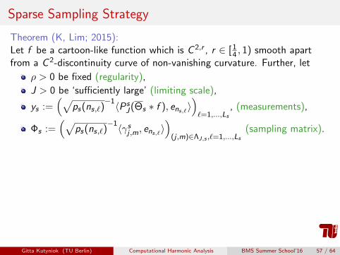
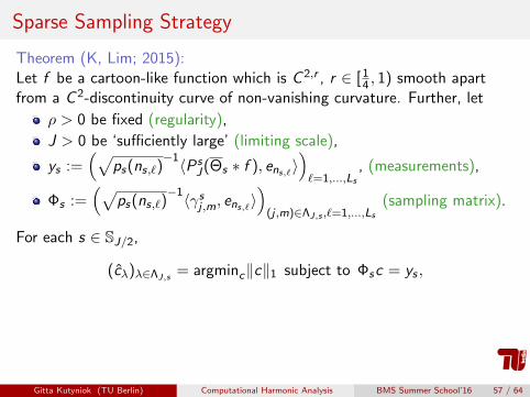
Sparse Sampling Strategy
Theorem (K, Lim; 2015):Let f be a cartoon-like function which is C 2,r , r ∈ [ 1
4 , 1) smooth apartfrom a C 2-discontinuity curve of non-vanishing curvature. Further, let
ρ > 0 be fixed (regularity),
J > 0 be ‘sufficiently large’ (limiting scale),
ys :=(√
ps(ns,`)−1〈Ps
J(Θs ∗ f ), ens,`〉)`=1,...,Ls
, (measurements),
Φs :=(√
ps(ns,`)−1〈γsj ,m, ens,`〉
)(j ,m)∈ΛJ,s ,`=1,...,Ls
(sampling matrix).
For each s ∈ SJ/2, (∑
s∈SJ/2Ls . J2J/2(1+2ρ) =: N)
(cλ)λ∈ΛJ,s= argminc‖c‖1 subject to Φsc = ys ,
Then with probability at least 1− 2−J ,∥∥∥f − ∑s∈SJ/2
∑λ∈ΛJ,s
cλψλ
∥∥∥2
2. 2−J(1−13ρ/2) as J →∞.
Gitta Kutyniok (TU Berlin) Computational Harmonic Analysis BMS Summer School’16 57 / 64
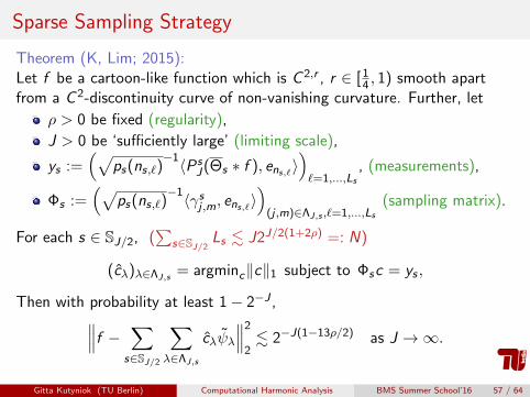
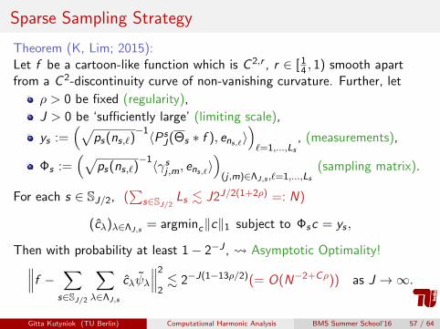
Sparse Sampling Strategy
Theorem (K, Lim; 2015):Let f be a cartoon-like function which is C 2,r , r ∈ [ 1
4 , 1) smooth apartfrom a C 2-discontinuity curve of non-vanishing curvature. Further, let
ρ > 0 be fixed (regularity),
J > 0 be ‘sufficiently large’ (limiting scale),
ys :=(√
ps(ns,`)−1〈Ps
J(Θs ∗ f ), ens,`〉)`=1,...,Ls
, (measurements),
Φs :=(√
ps(ns,`)−1〈γsj ,m, ens,`〉
)(j ,m)∈ΛJ,s ,`=1,...,Ls
(sampling matrix).
For each s ∈ SJ/2, (∑
s∈SJ/2Ls . J2J/2(1+2ρ) =: N)
(cλ)λ∈ΛJ,s= argminc‖c‖1 subject to Φsc = ys ,
Then with probability at least 1− 2−J , Asymptotic Optimality!∥∥∥f − ∑s∈SJ/2
∑λ∈ΛJ,s
cλψλ
∥∥∥2
2. 2−J(1−13ρ/2)(= O(N−2+Cρ)) as J →∞.
Gitta Kutyniok (TU Berlin) Computational Harmonic Analysis BMS Summer School’16 57 / 64
Numerical Experiments
Gitta Kutyniok (TU Berlin) Computational Harmonic Analysis BMS Summer School’16 58 / 64
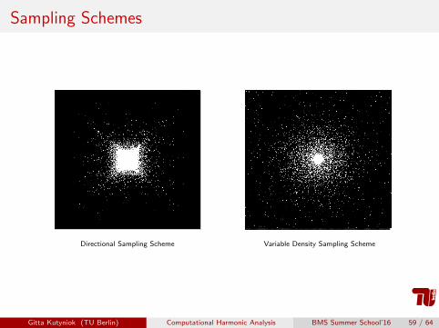
Sampling Schemes
Directional Sampling Scheme Variable Density Sampling Scheme
Gitta Kutyniok (TU Berlin) Computational Harmonic Analysis BMS Summer School’16 59 / 64
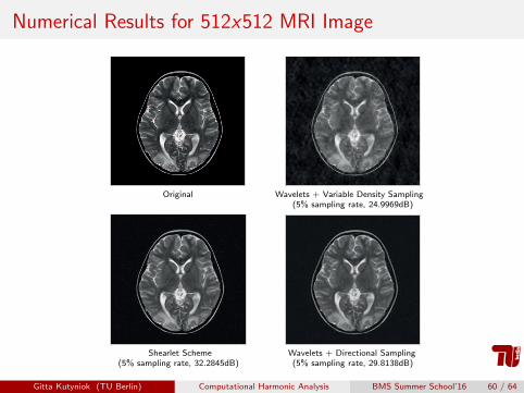
Numerical Results for 512x512 MRI Image
Shearlet Scheme(5% sampling rate, 32.2845dB)
Wavelets + Directional Sampling(5% sampling rate, 29.8138dB)
Original Wavelets + Variable Density Sampling(5% sampling rate, 24.9969dB)
Gitta Kutyniok (TU Berlin) Computational Harmonic Analysis BMS Summer School’16 60 / 64

Approximation Curves for 512x512 MRI Image
0 5 10 15 20 2520
25
30
35
40
45
sampling rate (%)
PS
NR
(dB
)
shear08
shear16
shear
wave02
wave01
0 5 10 15 20 250
100
200
300
400
500
600
sampling rate (%)
run
nin
g tim
e (
se
c)
shear08
shear16
shear
wave02
wave01
shear08: Directional sampling scheme with 8 directional filters.
shear16: Directional sampling scheme with 16 directional filters.
shear: Directional sampling scheme with (normal) shearlets.
wave02: Directional sampling scheme with wavelets.
wave01: Variable density sampling scheme with wavelets.
Gitta Kutyniok (TU Berlin) Computational Harmonic Analysis BMS Summer School’16 61 / 64

Let’s conclude...
Gitta Kutyniok (TU Berlin) Computational Harmonic Analysis BMS Summer School’16 62 / 64

What to take Home...?
Computational harmonic analysis and sparse approximation are apowerful combination to solve ill-posed inverse problems in imaging.
Such a sparse regularization approach allows also precise theoreticalresults.
We discussed the following inverse problems:I Feature ExtractionI Magnetic Resonance Imaging
Further applications include:I InpaintingI Edge DetectionI ...
Gitta Kutyniok (TU Berlin) Computational Harmonic Analysis BMS Summer School’16 63 / 64
THANK YOU!
References available at:
www.math.tu-berlin.de/∼kutyniokCode available at:
www.ShearLab.org
Related Books:
Y. Eldar and G. KutyniokCompressed Sensing: Theory and ApplicationsCambridge University Press, 2012.G. Kutyniok and D. LabateShearlets: Multiscale Analysis for Multivariate DataBirkhauser-Springer, 2012.
Gitta Kutyniok (TU Berlin) Computational Harmonic Analysis BMS Summer School’16 64 / 64