When Harmonic Analysis Meets Machine Learning: Lipschitz ...rvbalan/PRESENTATIONS/ieee2017.pdfWhen...
59
When Harmonic Analysis Meets Machine Learning: Lipschitz Analysis of Deep Convolution Networks Radu Balan Department of Mathematics, AMSC, CSCAMM and NWC University of Maryland, College Park, MD Joint work with Dongmian Zou (UMD), Maneesh Singh (Verisk) October 10, 2017 IEEE Computational Intelligence Society and Signal Processing Society University of Maryland, College Park, MD
Transcript of When Harmonic Analysis Meets Machine Learning: Lipschitz ...rvbalan/PRESENTATIONS/ieee2017.pdfWhen...

When Harmonic Analysis Meets Machine Learning:Lipschitz Analysis of Deep Convolution Networks
Radu Balan
Department of Mathematics, AMSC, CSCAMM and NWCUniversity of Maryland, College Park, MD
Joint work with Dongmian Zou (UMD), Maneesh Singh (Verisk)
October 10, 2017IEEE Computational Intelligence Society and Signal Processing Society
University of Maryland, College Park, MD

”This material is based upon work supported by the National ScienceFoundation under Grant No. DMS-1413249. Any opinions, findings, andconclusions or recommendations expressed in this material are those of theauthor(s) and do not necessarily reflect the views of the National ScienceFoundation.” The author has been partially supported by ARO under grantW911NF1610008 and LTS under grant H9823013D00560049.

Table of Contents:
1 Three Examples
2 Problem Formulation
3 Deep Convolutional Neural Networks
4 Lipschitz Analysis
5 Numerical Results

Three Examples Problem Formulation Deep Convolutional Neural Networks Lipschitz Analysis Numerical Results
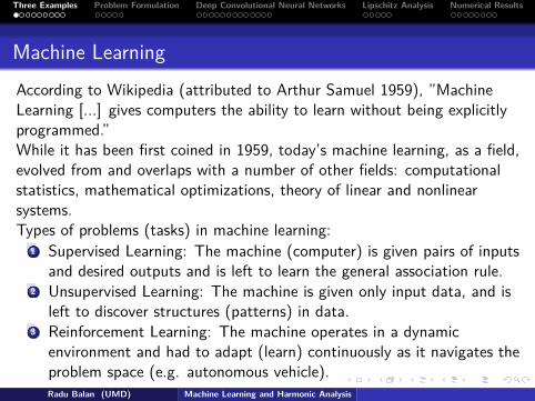
Machine LearningAccording to Wikipedia (attributed to Arthur Samuel 1959), ”MachineLearning [...] gives computers the ability to learn without being explicitlyprogrammed.”While it has been first coined in 1959, today’s machine learning, as a field,evolved from and overlaps with a number of other fields: computationalstatistics, mathematical optimizations, theory of linear and nonlinearsystems.
Types of problems (tasks) in machine learning:1 Supervised Learning: The machine (computer) is given pairs of inputs
and desired outputs and is left to learn the general association rule.2 Unsupervised Learning: The machine is given only input data, and is
left to discover structures (patterns) in data.3 Reinforcement Learning: The machine operates in a dynamic
environment and had to adapt (learn) continuously as it navigates theproblem space (e.g. autonomous vehicle).
Radu Balan (UMD) Machine Learning and Harmonic Analysis
Three Examples Problem Formulation Deep Convolutional Neural Networks Lipschitz Analysis Numerical Results
Machine LearningAccording to Wikipedia (attributed to Arthur Samuel 1959), ”MachineLearning [...] gives computers the ability to learn without being explicitlyprogrammed.”While it has been first coined in 1959, today’s machine learning, as a field,evolved from and overlaps with a number of other fields: computationalstatistics, mathematical optimizations, theory of linear and nonlinearsystems.Types of problems (tasks) in machine learning:
1 Supervised Learning: The machine (computer) is given pairs of inputsand desired outputs and is left to learn the general association rule.
2 Unsupervised Learning: The machine is given only input data, and isleft to discover structures (patterns) in data.
3 Reinforcement Learning: The machine operates in a dynamicenvironment and had to adapt (learn) continuously as it navigates theproblem space (e.g. autonomous vehicle).Radu Balan (UMD) Machine Learning and Harmonic Analysis

Three Examples Problem Formulation Deep Convolutional Neural Networks Lipschitz Analysis Numerical Results
Example 1: The AlexNetThe ImageNet Dataset
Dataset: ImageNet dataset [DDSLLF09]. Currently (2017): 14.2mil.images; 21841 categories; image-net.orgTask: Classify an input image, i.e. place it into one category.
Figure: The ”ostrich” category ”Struthio Camelus” 1393 pictures. Fromimage-net.org
Radu Balan (UMD) Machine Learning and Harmonic Analysis

Three Examples Problem Formulation Deep Convolutional Neural Networks Lipschitz Analysis Numerical Results
Example 1: The AlexNetThe Supervised Machine Learning
The AlexNet is 8 layer network, 5 convolutive layers plus 3 dense layers.Introduced by (Alex) Krizhevsky, Sutskever and Hinton in 2012 [KSH12].Trained on a subset of the ImageNet: Part of the ImageNet Large ScaleVisual Recognition Challenge 2010-2012: 1000 object classes and1,431,167 images.
Figure: From Krizhevsky et all 2012 [KSH12]: AlexNet: 5 convolutive layers + 3dense layers. Input size: 224x224x3 pixels. Output size: 1000.
Radu Balan (UMD) Machine Learning and Harmonic Analysis

Three Examples Problem Formulation Deep Convolutional Neural Networks Lipschitz Analysis Numerical Results
Example 1: The AlexNetAdversarial Perturbations
The authors of [SZSBEGF13] (Szegedy, Zaremba, Sutskever, Bruna,Erhan, Goodfellow, Fergus, ’Intriguing properties ...’) found smallvariations of the input, almost imperceptible, that produced completelydifferent classification decisions:
Figure: From Szegedy et all 2013 [SZSBEGF13]: AlexNet: 6 different classes:original image, difference, and adversarial example – all classified as ’ostrich’
Radu Balan (UMD) Machine Learning and Harmonic Analysis

Three Examples Problem Formulation Deep Convolutional Neural Networks Lipschitz Analysis Numerical Results
Example 1: The AlexNetLipschitz Analysis
Szegedy et all 2013 [SZSBEGF13] computed the Lipschitz constants ofeach layer.
Layer Size Sing.ValConv. 1 3× 11× 11× 96 20Conv. 2 96× 5× 5× 256 10Conv. 3 256× 3× 3× 384 7Conv. 4 384× 3× 3× 384 7.3Conv. 5 384× 3× 3× 256 11
Fully Conn.1 9216(43264)× 4096 3.12Fully Conn.2 4096× 4096 4Fully Conn.3 4096× 1000 4
Overall Lipschitz constant:
Lip ≤ 20 ∗ 10 ∗ 7 ∗ 7.3 ∗ 11 ∗ 3.12 ∗ 4 ∗ 4 = 5, 612, 006Radu Balan (UMD) Machine Learning and Harmonic Analysis
Three Examples Problem Formulation Deep Convolutional Neural Networks Lipschitz Analysis Numerical Results
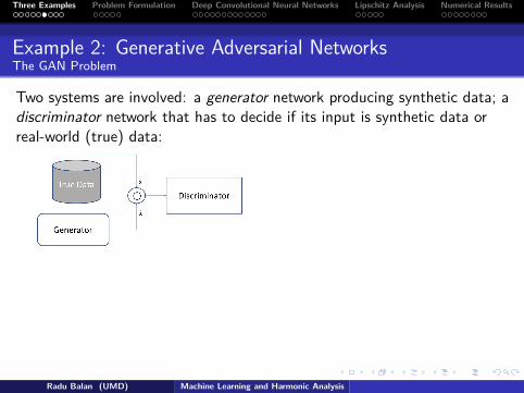
Example 2: Generative Adversarial NetworksThe GAN Problem
Two systems are involved: a generator network producing synthetic data; adiscriminator network that has to decide if its input is synthetic data orreal-world (true) data:
Introduced by Goodfellow et al[GPMXWOCB14] in 2014, GANssolve a minimax optimization prob-lem:
minG
maxD
Ex∼Pr [log(D(x))] + Ex∼Pg [log(1− D(x))]
where Pr is the distribution of true data, Pg is the generator distribution,and D : x 7→ D(x) ∈ [0, 1] is the discriminator map (1 for likely true data;0 for likely synthetic data).
Radu Balan (UMD) Machine Learning and Harmonic Analysis

Three Examples Problem Formulation Deep Convolutional Neural Networks Lipschitz Analysis Numerical Results
Example 2: Generative Adversarial NetworksThe Wasserstein Optimization Problem
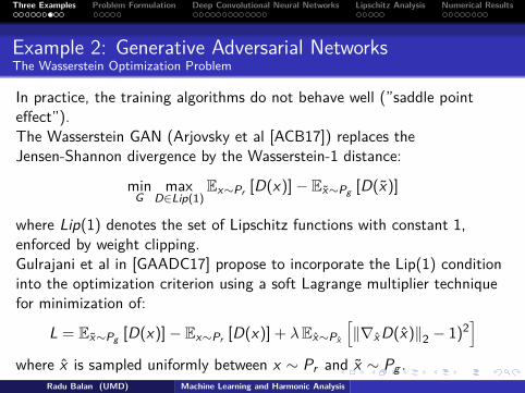
In practice, the training algorithms do not behave well (”saddle pointeffect”).The Wasserstein GAN (Arjovsky et al [ACB17]) replaces theJensen-Shannon divergence by the Wasserstein-1 distance:
minG
maxD∈Lip(1)
Ex∼Pr [D(x)]− Ex∼Pg [D(x)]
where Lip(1) denotes the set of Lipschitz functions with constant 1,enforced by weight clipping.
Gulrajani et al in [GAADC17] propose to incorporate the Lip(1) conditioninto the optimization criterion using a soft Lagrange multiplier techniquefor minimization of:
L = Ex∼Pg [D(x)]− Ex∼Pr [D(x)] + λEx∼Px
[‖∇x D(x)‖2 − 1)2
]where x is sampled uniformly between x ∼ Pr and x ∼ Pg .
Radu Balan (UMD) Machine Learning and Harmonic Analysis
Three Examples Problem Formulation Deep Convolutional Neural Networks Lipschitz Analysis Numerical Results
Example 2: Generative Adversarial NetworksThe Wasserstein Optimization Problem
In practice, the training algorithms do not behave well (”saddle pointeffect”).The Wasserstein GAN (Arjovsky et al [ACB17]) replaces theJensen-Shannon divergence by the Wasserstein-1 distance:
minG
maxD∈Lip(1)
Ex∼Pr [D(x)]− Ex∼Pg [D(x)]
where Lip(1) denotes the set of Lipschitz functions with constant 1,enforced by weight clipping.Gulrajani et al in [GAADC17] propose to incorporate the Lip(1) conditioninto the optimization criterion using a soft Lagrange multiplier techniquefor minimization of:
L = Ex∼Pg [D(x)]− Ex∼Pr [D(x)] + λEx∼Px
[‖∇x D(x)‖2 − 1)2
]where x is sampled uniformly between x ∼ Pr and x ∼ Pg .
Radu Balan (UMD) Machine Learning and Harmonic Analysis

Three Examples Problem Formulation Deep Convolutional Neural Networks Lipschitz Analysis Numerical Results
Example 3: The Scattering NetworkTopology
Example of Scattering Network; definition and properties: [Mallat12]; thisexample from [BSZ17]:
Input: f ; Outputs: y = (yl ,k).Radu Balan (UMD) Machine Learning and Harmonic Analysis

Three Examples Problem Formulation Deep Convolutional Neural Networks Lipschitz Analysis Numerical Results
Example 3: Scattering NetworkLipschitz Analysis
Remarks:Outputs from each layer
Tree-like topologyBackpropagation/Chain rule:Lipschitz bound 40.Mallat’s result predicts Lip = 1.
Radu Balan (UMD) Machine Learning and Harmonic Analysis

Three Examples Problem Formulation Deep Convolutional Neural Networks Lipschitz Analysis Numerical Results
Example 3: Scattering NetworkLipschitz Analysis
Remarks:Outputs from each layerTree-like topology
Backpropagation/Chain rule:Lipschitz bound 40.Mallat’s result predicts Lip = 1.
Radu Balan (UMD) Machine Learning and Harmonic Analysis

Three Examples Problem Formulation Deep Convolutional Neural Networks Lipschitz Analysis Numerical Results
Example 3: Scattering NetworkLipschitz Analysis
Remarks:Outputs from each layerTree-like topologyBackpropagation/Chain rule:Lipschitz bound 40.
Mallat’s result predicts Lip = 1.
Radu Balan (UMD) Machine Learning and Harmonic Analysis

Three Examples Problem Formulation Deep Convolutional Neural Networks Lipschitz Analysis Numerical Results
Example 3: Scattering NetworkLipschitz Analysis
Remarks:Outputs from each layerTree-like topologyBackpropagation/Chain rule:Lipschitz bound 40.Mallat’s result predicts Lip = 1.
Radu Balan (UMD) Machine Learning and Harmonic Analysis

Three Examples Problem Formulation Deep Convolutional Neural Networks Lipschitz Analysis Numerical Results
Problem FormulationNonlinear Maps
Consider a nonlinear function between two metric spaces,
F : (X , dX )→ (Y , dY ).
Radu Balan (UMD) Machine Learning and Harmonic Analysis

Three Examples Problem Formulation Deep Convolutional Neural Networks Lipschitz Analysis Numerical Results
Problem FormulationLipschitz analysis of nonlinear systems
F : (X , dX )→ (Y , dY )
F is called Lipschitz with constant C if for any f , f ∈ X ,
dY (F(f ),F(f )) ≤ C dX (f , f )
The optimal (i.e. smallest) Lipschitz constant is denoted Lip(F). Thesquare C2 is called Lipschitz bound (similar to the Bessel bound).
F is called bi-Lipschitz with constants C1,C2 > 0 if for any f , f ∈ X ,
C1 dX (f , f ) ≤ dY (F(f ),F(f )) ≤ C2 dX (f , f )
The square C21 ,C2
2 are called Lipschitz bounds (similar to frame bounds).
Radu Balan (UMD) Machine Learning and Harmonic Analysis

Three Examples Problem Formulation Deep Convolutional Neural Networks Lipschitz Analysis Numerical Results
Problem FormulationMotivating Examples
Consider the typical neural network as a feature extractor component in aclassification system:
g = F(f ) = FM(...F1(f ; W1, ϕ1); ...; WM , ϕM)Fm(f ; Wm, ϕm) = ϕm(Wmf )
Wm is a linear operator (matrix); ϕm is a Lip(1) scalar nonlinearity (e.g.Rectified Linear Unit).
Radu Balan (UMD) Machine Learning and Harmonic Analysis

Three Examples Problem Formulation Deep Convolutional Neural Networks Lipschitz Analysis Numerical Results
Problem FormulationProblem 1
Given a deep network:
Estimate the Lipschitz constant, or bound:
Lip = supf 6=f ∈L2
‖y − y‖2‖f − f ‖2
, Bound = supf 6=f ∈L2
‖y − y‖22‖f − f ‖22
.
Methods (Approaches):1 Standard Method: Backpropagation, or chain-rule2 New Method: Storage function based approach (dissipative systems)3 Numerical Method: Simulations
Radu Balan (UMD) Machine Learning and Harmonic Analysis

Three Examples Problem Formulation Deep Convolutional Neural Networks Lipschitz Analysis Numerical Results
Problem FormulationProblem 2
Given a deep network:
Estimate the stability of the output to specific variations of the input:1 Invariance to deformations: f (x) = f (x − τ(x)), for some smooth τ .2 Covariance to such deformations f (x) = f (x − τ(x)), for smooth τ
and bandlimited signals f ;3 Tail bounds when f has a known statistical distribution (e.g. normal
with known spectral power)
Radu Balan (UMD) Machine Learning and Harmonic Analysis
Three Examples Problem Formulation Deep Convolutional Neural Networks Lipschitz Analysis Numerical Results
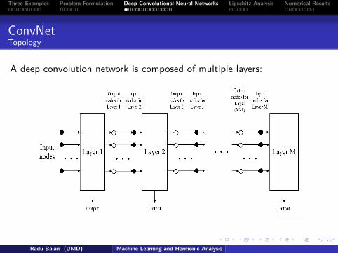
ConvNetTopology
A deep convolution network is composed of multiple layers:
Radu Balan (UMD) Machine Learning and Harmonic Analysis

Three Examples Problem Formulation Deep Convolutional Neural Networks Lipschitz Analysis Numerical Results
ConvNetOne Layer
Each layer is composed of two or three sublayers: convolution,downsampling, detection/pooling/merge.
Radu Balan (UMD) Machine Learning and Harmonic Analysis

Three Examples Problem Formulation Deep Convolutional Neural Networks Lipschitz Analysis Numerical Results
ConvNet: SublayersLinear Filters: Convolution and Pooling-to-Output Sublayer
f (2) = g ∗ f (1) , f (2)(x) =∫
g(x − ξ)f (1)(ξ)dξ
where g ∈ B = {g ∈ S ′ , g ∈ L∞(Rd )}.
(B, ∗) is a Banach algebra with norm ‖g‖B = ‖g‖∞.Notation: g for regular convolution filters, and Φ for pooling-to-outputfilters.
Radu Balan (UMD) Machine Learning and Harmonic Analysis

Three Examples Problem Formulation Deep Convolutional Neural Networks Lipschitz Analysis Numerical Results
ConvNet: SublayersDownsampling Sublayer
f (2)(x) = f (1)(Dx)
For f (1) ∈ L2(Rd ) and D = D0 · I, f (2) ∈ L2(Rd ) and
‖f (2)‖22 =∫Rd|f (2)(x)|2dx = 1
|det(D)|
∫Rd|f (1)(x)|2dx = 1
Dd0‖f (1)‖22
Radu Balan (UMD) Machine Learning and Harmonic Analysis

Three Examples Problem Formulation Deep Convolutional Neural Networks Lipschitz Analysis Numerical Results
ConvNet: SublayersDetection and Pooling Sublayer
We consider three types of detection/pooling/merge sublayers:Type I, τ1: Componentwise Addition: z =
∑kj=1 σj(yj)
Type II, τ2: p-norm aggregation: z =(∑k
j=1 |σj(yj)|p)1/p
Type III, τ3: Componentwise Multiplication: z =∏k
j=1 σj(yj)
Assumptions: (1) σj are scalar Lipschitz functions with Lip(σj) ≤ 1; (2) Ifσj is connected to a multiplication block then ‖σj‖∞ ≤ 1.
Radu Balan (UMD) Machine Learning and Harmonic Analysis
Three Examples Problem Formulation Deep Convolutional Neural Networks Lipschitz Analysis Numerical Results
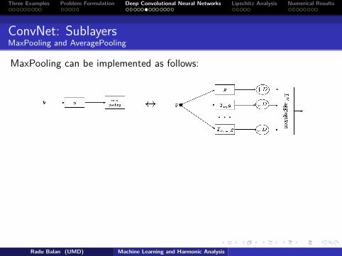
ConvNet: SublayersMaxPooling and AveragePooling
MaxPooling can be implemented as follows:
AveragePooling can be implemented as follows:
Radu Balan (UMD) Machine Learning and Harmonic Analysis

Three Examples Problem Formulation Deep Convolutional Neural Networks Lipschitz Analysis Numerical Results
ConvNet: SublayersMaxPooling and AveragePooling
MaxPooling can be implemented as follows:
AveragePooling can be implemented as follows:
Radu Balan (UMD) Machine Learning and Harmonic Analysis

Three Examples Problem Formulation Deep Convolutional Neural Networks Lipschitz Analysis Numerical Results
ConvNet: SublayersLong Short-Term Memory
Long Short-Term Memory (LSTM) networks [HS97, GSKSS15].By BiObserver - Own work, CC BY-SA 4.0,https://commons.wikimedia.org/w/index.php?curid=43992484
Radu Balan (UMD) Machine Learning and Harmonic Analysis

Three Examples Problem Formulation Deep Convolutional Neural Networks Lipschitz Analysis Numerical Results
ConvNet: Layer mComponents of the mth layer
Radu Balan (UMD) Machine Learning and Harmonic Analysis

Three Examples Problem Formulation Deep Convolutional Neural Networks Lipschitz Analysis Numerical Results
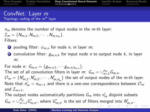
ConvNet: Layer mTopology coding of the mth layer
nm denotes the number of input nodes in the m-th layer:Im = {Nm,1,Nm,2, · · · ,Nm,nm}.Filters:
1 pooling filter: φm,n for node n, in layer m;2 convolution filter: gm,n,k for input node n to output node k, in layer
m;For node n: Gm,n = {gm,n;1, · · · gm,n;km,n}.The set of all convolution filters in layer m: Gm = ∪nm
n=1Gm,n.
Om = {N ′m,1,N ′m,2, · · · ,N ′m,n′m} the set of output nodes of the m-th layer.Note that n′m = nm+1 and there is a one-one correspondence between Omand Im+1.The output nodes automatically partitions Gm into n′m disjoint subsetsGm = ∪n′m
n′=1G ′m,n′ , where G ′m,n′ is the set of filters merged into N ′m,n′ .
Radu Balan (UMD) Machine Learning and Harmonic Analysis
Three Examples Problem Formulation Deep Convolutional Neural Networks Lipschitz Analysis Numerical Results
ConvNet: Layer mTopology coding of the mth layer
nm denotes the number of input nodes in the m-th layer:Im = {Nm,1,Nm,2, · · · ,Nm,nm}.Filters:
1 pooling filter: φm,n for node n, in layer m;2 convolution filter: gm,n,k for input node n to output node k, in layer
m;For node n: Gm,n = {gm,n;1, · · · gm,n;km,n}.The set of all convolution filters in layer m: Gm = ∪nm
n=1Gm,n.Om = {N ′m,1,N ′m,2, · · · ,N ′m,n′m} the set of output nodes of the m-th layer.Note that n′m = nm+1 and there is a one-one correspondence between Omand Im+1.The output nodes automatically partitions Gm into n′m disjoint subsetsGm = ∪n′m
n′=1G ′m,n′ , where G ′m,n′ is the set of filters merged into N ′m,n′ .
Radu Balan (UMD) Machine Learning and Harmonic Analysis

Three Examples Problem Formulation Deep Convolutional Neural Networks Lipschitz Analysis Numerical Results
ConvNet: Layer mTopology coding of the mth layer
For each filter gm,n;k , we define an associated multiplier lm,n;k in thefollowing way: suppose gm,n;k ∈ G ′m,k , let K =
∣∣∣G ′m,k ∣∣∣ denote thecardinality of G ′m,k . Then
lm,n;k ={
K , if gm,n;k ∈ τ1 ∪ τ3
K max{0,2/p−1} , if gm,n;k ∈ τ2(3.1)
Radu Balan (UMD) Machine Learning and Harmonic Analysis

Three Examples Problem Formulation Deep Convolutional Neural Networks Lipschitz Analysis Numerical Results
ConvNet: Layer mTopology coding of the mth layer
Radu Balan (UMD) Machine Learning and Harmonic Analysis

Three Examples Problem Formulation Deep Convolutional Neural Networks Lipschitz Analysis Numerical Results
ConvNet: Layer mTopology coding of the mth layer
Radu Balan (UMD) Machine Learning and Harmonic Analysis

Three Examples Problem Formulation Deep Convolutional Neural Networks Lipschitz Analysis Numerical Results
ConvNet: Layer mTopology coding of the mth layer
Radu Balan (UMD) Machine Learning and Harmonic Analysis

Three Examples Problem Formulation Deep Convolutional Neural Networks Lipschitz Analysis Numerical Results
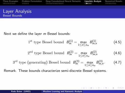
Layer AnalysisBessel Bounds
In each layer m and for each input node n we define three types of Besselbounds:
1st type Bessel bound:
B(1)m,n = ‖
∣∣∣φm,n∣∣∣2 +
∑gm,n;k∈Gm,n
lm,n;kD−dm,n;k |gm,n;k |2 ‖
∞
(4.2)
2nd type Bessel bound:
B(2)m,n = ‖
∑gm,n;k∈Gm,n
lm,n;kD−dm,n;k |gm,n;k |2 ‖
∞
(4.3)
3rd type (or generating) bound:
B(3)m,n = ‖φm,n‖
2∞ . (4.4)
Radu Balan (UMD) Machine Learning and Harmonic Analysis
Three Examples Problem Formulation Deep Convolutional Neural Networks Lipschitz Analysis Numerical Results
Layer AnalysisBessel Bounds
Next we define the layer m Bessel bounds:
1st type Bessel bound B(1)m = max
1≤n≤nmB(1)
m,n (4.5)
2nd type Bessel bound B(2)m = max
1≤n≤nmB(2)
m,n (4.6)
3rd type (generating) Bessel bound B(3)m = max
1≤n≤nmB(3)
m,n. (4.7)
Remark. These bounds characterize semi-discrete Bessel systems.
Radu Balan (UMD) Machine Learning and Harmonic Analysis

Three Examples Problem Formulation Deep Convolutional Neural Networks Lipschitz Analysis Numerical Results
Lipschitz AnalysisFirst Result
Theorem[BSZ17] Consider a Convolutional Neural Network with M layers asdescribed before, where all scalar nonlinear functions are Lipschitz withLip(ϕm,n,n′) ≤ 1. Additionally, those ϕm,n,n′ that aggregate into amultiplicative block satisfy ‖ϕm,n,n′‖∞ ≤ 1. Let the m-th layer 1st typeBessel bound be
B(1)m = max
1≤n≤nm‖∣∣∣φm,n
∣∣∣2 +km,n∑k=1
lm,n;kD−dm,n;k |gm,n;k |2 ‖
∞
.
Then the Lipschitz bound of the entire CNN is upper bounded by∏Mm=1 max(1,B(1)
m ). Specifically, for any f , f ∈ L2(Rd ):
‖F(f )−F(f )‖22 ≤( M∏
m=1max(1,B(1)
m ))‖f − f ‖22,
Radu Balan (UMD) Machine Learning and Harmonic Analysis

Three Examples Problem Formulation Deep Convolutional Neural Networks Lipschitz Analysis Numerical Results
Lipschitz AnalysisSecond Result
TheoremConsider a Convolutional Neural Network with M layers as describedbefore, where all scalar nonlinearities satisfy the same conditions as in theprevious result. For layer m, let B(1)
m , B(2)m , and B(3)
m denote the threeBessel bounds defined earlier. Denote by L the optimal solution of thefollowing linear program:
Γ = maxy1,...,yM ,z1,...,zM≥0
M∑m=1
zm
s.t. y0 = 1ym + zm ≤ B(1)
m ym−1, 1 ≤ m ≤ Mym ≤ B(2)
m ym−1, 1 ≤ m ≤ Mzm ≤ B(3)
m ym−1, 1 ≤ m ≤ M
(4.8)
Radu Balan (UMD) Machine Learning and Harmonic Analysis

Three Examples Problem Formulation Deep Convolutional Neural Networks Lipschitz Analysis Numerical Results
Lipschitz AnalysisSecond Result - cont’d
TheoremThen the Lipschitz bound satisfies Lip(F)2 ≤ Γ. Specifically, for anyf , f ∈ L2(Rd ):
‖F(f )−F(f )‖22 ≤ Γ‖f − f ‖22,
Radu Balan (UMD) Machine Learning and Harmonic Analysis

Three Examples Problem Formulation Deep Convolutional Neural Networks Lipschitz Analysis Numerical Results
Example 1: Scattering Network
The Lipschitz constant:Backpropagation/Chain rule:Lipschitz bound 40 (henceLip ≤ 6.3).
Using our main theorem,Lip ≤ 1, but Mallat’s result:Lip = 1.
Filters have been choosen as in adyadic wavelet decomposition. ThusB(1)
m = B(2)m = B(3)
m = 1, 1 ≤ m ≤ 4.
Radu Balan (UMD) Machine Learning and Harmonic Analysis

Three Examples Problem Formulation Deep Convolutional Neural Networks Lipschitz Analysis Numerical Results
Example 1: Scattering Network
The Lipschitz constant:Backpropagation/Chain rule:Lipschitz bound 40 (henceLip ≤ 6.3).Using our main theorem,Lip ≤ 1, but Mallat’s result:Lip = 1.
Filters have been choosen as in adyadic wavelet decomposition. ThusB(1)
m = B(2)m = B(3)
m = 1, 1 ≤ m ≤ 4.
Radu Balan (UMD) Machine Learning and Harmonic Analysis
Three Examples Problem Formulation Deep Convolutional Neural Networks Lipschitz Analysis Numerical Results
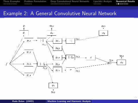
Example 2: A General Convolutive Neural Network
Radu Balan (UMD) Machine Learning and Harmonic Analysis

Three Examples Problem Formulation Deep Convolutional Neural Networks Lipschitz Analysis Numerical Results
Example 2: A General Convolutive Neural NetworkSet p = 2 and:
F (ω) = exp(4ω2 + 4ω + 1
4ω2 + 4ω)χ(−1,−1/2)(ω) + χ(−1/2,1/2)(ω) + exp(
4ω2 − 4ω + 14ω2 − 4ω
)χ(1/2,1)(ω).
φ1(ω) = F (ω)g1,j (ω) = F (ω + 2j − 1/2) + F (ω − 2j + 1/2) , j = 1, 2, 3, 4
φ2(ω) = exp(4ω2 + 12ω + 94ω2 + 12ω + 8
)χ(−2,−3/2)(ω) +
χ(−3/2,3/2)(ω) + exp(4ω2 − 12ω + 94ω2 − 12ω + 8
)χ(3/2,2)(ω)
g2,j (ω) = F (ω + 2j) + F (ω − 2j) , j = 1, 2, 3g2,4(ω) = F (ω + 2) + F (ω − 2)g2,5(ω) = F (ω + 5) + F (ω − 5)
φ3(ω) = exp(4ω2 + 20ω + 254ω2 + 20ω + 24
)χ(−3,−5/2)(ω) +
χ(−5/2,5/2)(ω) + exp(4ω2 − 20ω + 254ω2 − 20ω + 25
)χ(5/2,3)(ω).
Radu Balan (UMD) Machine Learning and Harmonic Analysis

Three Examples Problem Formulation Deep Convolutional Neural Networks Lipschitz Analysis Numerical Results
Example 2: A General Convolutive Neural Network
Bessel Bounds: B(1)m = 2e−1/3 =
1.43, B(2)m = B(3)
m = 1.The Lipschitz bound:
Usingbackpropagation/chain-rule:Lip2 ≤ 5.Using Theorem 1:Lip2 ≤ 2.9430.Using Theorem 2 (linearprogram): Lip2 ≤ 2.2992.
Radu Balan (UMD) Machine Learning and Harmonic Analysis

Three Examples Problem Formulation Deep Convolutional Neural Networks Lipschitz Analysis Numerical Results
Example 3: Lipschitz constant as an optimization criterionNonlinear Discriminant Analysis
In Linear Discriminant Analysis (LDA), the objective is to maximize the”separation” between two classes, while controlling the variances withinclass.A similar nonlinear discriminant can be defined:
S = ‖E[F(f )|f ∈ C1]− E[F(f )|f ∈ C2]‖2
‖Cov(F(f )|f ∈ C1)‖F + ‖Cov(F(f )|f ∈ C2)‖F.
Replace the statistics ‖Cov‖F by Lipschitz bounds:Lipschitz bound based separation:
S = ‖E[F(f )|f ∈ C1]− E[F(f )|f ∈ C2]‖2
Lip21 + Lip2
2.
Radu Balan (UMD) Machine Learning and Harmonic Analysis

Three Examples Problem Formulation Deep Convolutional Neural Networks Lipschitz Analysis Numerical Results
Example 3: Lipschitz constant as an optimization criterionNonlinear Discriminant Analysis
The Lipschitz bounds Lip21 , Lip2
2 are computed using Gaussian generativemodels for the two classes: (µc ,WcW T
c ), where Wc represents thewhitening filter for class c ∈ {1, 2}.
Radu Balan (UMD) Machine Learning and Harmonic Analysis

Three Examples Problem Formulation Deep Convolutional Neural Networks Lipschitz Analysis Numerical Results
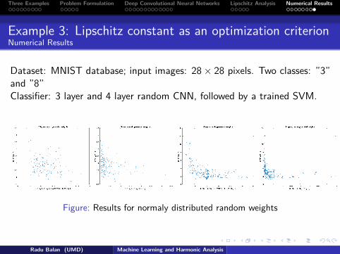
Example 3: Lipschitz constant as an optimization criterionNumerical Results
Dataset: MNIST database; input images: 28× 28 pixels. Two classes: ”3”and ”8”Classifier: 3 layer and 4 layer random CNN, followed by a trained SVM.
Figure: Results for uniformly distributed random weights
Conclusion: The error rate decreases as the Lipschitz bound separationincreases. The discriminant spread is wider.
Radu Balan (UMD) Machine Learning and Harmonic Analysis
Three Examples Problem Formulation Deep Convolutional Neural Networks Lipschitz Analysis Numerical Results
Example 3: Lipschitz constant as an optimization criterionNumerical Results
Dataset: MNIST database; input images: 28× 28 pixels. Two classes: ”3”and ”8”Classifier: 3 layer and 4 layer random CNN, followed by a trained SVM.
Figure: Results for normaly distributed random weights
Radu Balan (UMD) Machine Learning and Harmonic Analysis

Three Examples Problem Formulation Deep Convolutional Neural Networks Lipschitz Analysis Numerical Results
References[ACB17] M. Arjovsky, S. Chintala, L. Bottou, Wasserstein GAN,online arXive:1701.07875, 2017.[BSZ17] Radu Balan, Manish Singh, Dongmian Zou, LipschitzProperties for Deep Convolutional Networks, available online arXiv1701.01527 [cs.LG], 18 Jan 2017.
[BZ15] Radu Balan, Dongmian Zou, On Lipschitz Analysis andLipschitz Synthesis for the Phase Retrieval Problem, available onlinearXiv 1506.02092v1 [mathFA], 6 June 2015; Lin. Alg. and Appl. 496(2016), 152-181.
[BGC16] Yoshua Bengio, Ian Goodfellow and Aaron Courville, Deeplearning, MIT Press, 2016.
[BM13] Joan Bruna and Stephane Mallat, Invariant scatteringconvolution networks, IEEE Transactions on Pattern Analysis andMachine Intelligence 35 (2013), no. 8, 1872–1886.Radu Balan (UMD) Machine Learning and Harmonic Analysis

Three Examples Problem Formulation Deep Convolutional Neural Networks Lipschitz Analysis Numerical Results
[BCLPS15] Joan Bruna, Soumith Chintala, Yann LeCun, SerkanPiantino, Arthur Szlam, and Mark Tygert, A theoretical argument forcomplex-valued convolutional networks, CoRR abs/1503.03438(2015).
[DDSLLF09] Jia Deng,Wei Dong, Richard Socher, Li-Jia Li, Kai Li,and Li Fei-Fei Imagenet: A large-scale hierarchical image database,IEEE Conference on Computer Vision and Pattern Recognition, CVPR2009, 248–255. 2009.[GPMXWOCB14] I. Goodfellow, J. Pouget-Abadie, M. Mirza, B. Xu,W. Warde-Farley, S. Ozair, A. Courville, Y. Bengio, GenerativeAdverserial Nets, Advances in Neural Information Processing Systems,2672–2680, 2014.[GSKSS15] Klaus Greff, Rupesh K. Srivastava, Jan Koutnik, Bas R.Steunebrink, Jurgen Schmidhuber, LSTM: A Search Space Odyssey,arXiv:1503.04069v1 [cs.NE], 13 Mar. 2015.
Radu Balan (UMD) Machine Learning and Harmonic Analysis

Three Examples Problem Formulation Deep Convolutional Neural Networks Lipschitz Analysis Numerical Results
[GAADC17] I. Gulrajani, F. Ahmed, M. Arjovsky, V. Dumoulin, A.Courville, Improved Training of Wasserstein GANs, onlinearXiv:1704.00028 [cs.LG], 29 May 2017.
[HS97] Sepp Hochreiter and Jurgen Schmidhuber, Long short-termmemory, Neural Comput. 9 (1997), no. 8, 1735–1780.
[KSH12] Alex Krizhevsky, Ilya Sutskever, and Geoff Hinton, Imagenetclassification with deep convolutional neural networks, Advances inNeural Information Processing Systems 25, 1106–1114, 2012.
[LBH15] Yann Lecun, Yoshua Bengio, and Geoffrey Hinton, Deeplearning, Nature 521 (2015), no. 7553, 436–444.
[LSS14] Roi Livni, Shai Shalev-Shwartz, and Ohad Shamir, On thecomputational efficiency of training neural networks, Advances inNeural Information Processing Systems 27 (Z. Ghahramani,M. Welling, C. Cortes, N.d. Lawrence, and K.q. Weinberger, eds.),Curran Associates, Inc., 2014, pp. 855–863.Radu Balan (UMD) Machine Learning and Harmonic Analysis

Three Examples Problem Formulation Deep Convolutional Neural Networks Lipschitz Analysis Numerical Results
[Mallat12] Stephane Mallat, Group invariant scattering,Communications on Pure and Applied Mathematics 65 (2012), no. 10,1331–1398.[SVS15] Tara N. Sainath, Oriol Vinyals, Andrew W. Senior, and HasimSak, Convolutional, long short-term memory, fully connected deepneural networks, 2015 IEEE International Conference on Acoustics,Speech and Signal Processing, ICASSP 2015, South Brisbane,Queensland, Australia, April 19-24, 2015, 2015, pp. 4580–4584.
[SLJSRAEVR15] Christian Szegedy, Wei Liu, Yangqing Jia, PierreSermanet, Scott Reed, Dragomir Angelov, Dumitru Erhan, VincentVanhoucke, and Andrew Rabinovich, Going deeper with convolutions,CVPR 2015, 2015.[SZSBEGF13] Christian Szegedy, Wojciech Zaremba, Ilya Sutskever,Joan Bruna, Dumitru Erhan, Ian J. Goodfellow, and Rob Fergus,
Radu Balan (UMD) Machine Learning and Harmonic Analysis

Three Examples Problem Formulation Deep Convolutional Neural Networks Lipschitz Analysis Numerical Results
Intriguing properties of neural networks, CoRR abs/1312.6199(2013).
[WB15a] Thomas Wiatowski and Helmut Bolcskei, Deep convolutionalneural networks based on semi-discrete frames, Proc. of IEEEInternational Symposium on Information Theory (ISIT), June 2015,pp. 1212–1216.
[WB15b]Thomas Wiatowski and Helmut Bolcskei, A mathematicaltheory of deep convolutional neural networks for feature extraction,IEEE Transactions on Information Theory (2015).
Radu Balan (UMD) Machine Learning and Harmonic Analysis