Compressive Spectral Anomaly Detection

Vishwanath Saragadam†, Jian Wang†, Xin Li‡ and Aswin C. Sankaranarayanan†

† ECE Department, Carnegie Mellon University, Pittsburgh PA‡ ECE Department, Duke University, Durham NC

Abstract

We propose a novel compressive sensing imager for de-tecting anomalous spectral profiles in a scene. The sens-ing strategy models the background spectrum to lie on alow-dimensional subspace while assuming the anomalies toform a spatially-sparse set of spectral profiles different fromthe background. Our core contributions are in the form of atwo stage sensing mechanism: in the first stage, we estimatethe subspace for the spectrum of background by acquir-ing spectral measurements at a few randomly-selected pix-els. In the second stage, we acquire spatially-multiplexedspectral measurements of the scene. Projecting the spec-tral measurements on the complementary subspace createsa sparse matrix which is then recovered using a Multi-ple Measurement Vector problem. Theoretical analysis andsimulations show significant speed up in acquisition timeover other anomaly detection techniques. A lab prototypebased on a DMD and a visible spectrometer validates ourproposed imager.

1. IntroductionHyperspectral images measure light intensity in a scene

as a function of space and spectrum. The availability ofspectral measurements at each spatial location helps in iden-tifying material composition. This has found applications infacial recognition [18, 14], segmentation [23] , and numer-ous geoscience and remote sensing applications [9].

An important application of hyperspectral imaging is toidentify the presence of anomalous materials in a scene.When the materials of interest are present in trace quan-tities, it is common to model them as anomalous spectralsignatures [16]. The most common approach for hyperspec-tral anomaly detection is to represent the background usinga low-dimensional subspace. Subsequently, a spatial loca-tion or a “pixel” which cannot be represented accurately bythe background model is tagged as an anomaly. Estimationof the location of these anomalies typically requires acqui-sition of the complete hyperspectral image. Since typicalhyperspectral images are extremely high-dimensional, the

Figure 1: Anomaly detection is often used for geologi-cal surveillance. (left) False-color visualization of a 256 ×256 × 360 hyperspectral image of the Deepwater horizonspill [22] with oil spills denoted in gray and backgroundin dark blue. (right) Pixels with anomalous spectra are de-tected using the proposed sensing framework and marked inred. The results were obtained using 3500 × 360 measure-ments which is 1/18 the dimensionality of the image.

imaging effort is not only time consuming and also requireshighly sensitive and expensive sensor elements.

In this paper, we propose a novel sensing framework thatdirectly estimates the location of anomalous spectral sig-natures without sensing the entire hyperspectral image as-sociated with a scene. We model the hyperspectral imageas a sum of the background, assumed to be low-rank, andthe anomalies, assumed to be sparse. Under these model-ing assumptions, we estimate the locations of the anoma-lies using a computational camera that implements the fol-lowing two-stage approach. In the first stage, we builda low-dimensional subspace for the background spectrumby acquiring a spectral measurements at a few randomly-selected spatial locations in the scene. In the second stage,we obtain spatially-multiplexed spectral measurements ofthe scene and estimate the sparse anomalies by projectingout the subspace corresponding to the background spec-trum. Figure 1 shows estimation of 200 anomalous pix-els of oil spill in 256 × 256 × 360 Deepwater oil spill hy-perspectral image [22] with 3500 spectral measurements.Our algorithm recovers anomalies with very high accuracywith fewer measurements than the dimension of the signal.

1

Our sensing framework enables a significant reduction inthe number of measurements over competing schemes thatrequire the entire hyperspectral image, thereby providingsignificant speedups and efficiencies at acquisition time.

We make the following contributions in this paper.

• Novel sensing framework. We propose a sensing frame-work that detects anomalies directly with fewer measure-ments than the dimension of the hyperspectral image.

• Theoretical guarantees. We provide expressions for theminimum number of measurements and recovery accu-racy for our proposed sensing method.

• Validation with a lab prototype. We demonstrate theefficacy of our approach using a lab prototype that uses adigital micromirror device (DMD) for spatial modulationand a spectrometer for spectral measurements.

We also evaluate our technique, on synthetic data, againstthe classical Reed Xiaoli (RX) [21] detector as well as morerecent techniques that rely on compressive imaging underthe low rank and sparse signal model.

2. Prior workNotation. We denote vectors in bold font, scalars in smallletters and matrices in capital letters. The `0-norm of avector is the number of non-zero entries. Given a matrixX ∈ RM×N and an index set Ω ⊂ 1, 2, . . . , N, XΩ

represents a matrix of size RM×|Ω| formed by selectingcolumns of X corresponding to the elements of Ω. Thep,q-norm of a matrix is defined as

‖X‖p,q =

(N∑

n=1

‖xi‖qp

)1/q

.

Note that this is an entry-wise norm and is not to be con-fused with the induced matrix norms. Hence, ‖X‖2,2 is theFrobenius norm of a matrix, ‖X‖2,1 is the sum of `2-normsof columns, ‖X‖p,0 is the number of non-zero columns ofX and ‖X>‖p,0 is the number of non-zero rows ofX . Con-sider a signal x ∈ RJN , which can be reshaped into a J×Nmatrix,X . The vector x is called K-block sparse if the num-ber of non-zero columns in X is no more than K.

Compressive sensing (CS). CS aims at recovering a sig-nal from a set of linear measurements fewer than its dimen-sionality [3], i.e., we seek to acquire a signal x ∈ RN fromM N measurements, y = Φx + e, where Φ ∈ RM×N

is the sensing matrix, and e is the measurement noise. CSrelies on the sensed signal being sparse either canonicallyor under a linear transformation. In such a scenario, we canrecover the signal by solving

minx‖y − Φx‖2, ‖x‖0 ≤ K.

There are many approaches to solving this optimizationproblem, including convex relaxation techniques like BasisPursuit [24] and greedy techniques like Orthogonal Match-ing Pursuit [19] and CoSaMP [17]. This model is also calledthe single measurement vector (SMV) problem.

The multiple measurement vector (MMV) problem ex-tends the idea of sensing of sparse signals to a scenariowhere we sense multiple signals that share a common spar-sity pattern [10]. The MMV problem can be formulated as

Y = ΦX + E, ‖X>‖2,0 ≤ K,

with Y ∈ RM×Q,X ∈ RN×Q,Φ ∈ RM×N and E ∈RM×Q. Here, Y = [y1,y2, ...,yQ] are the multiple mea-surements, X = [x1,x2, ...,xQ] are the signals that sharethe same sparsity pattern, and E = [e1, e2, ..., eQ] is themeasurement noise. Solutions to the MMV problem canbe obtained through algorithms similar in spirit to the SMVproblem [10]. The MMV model and the results in Baraniuket al. [4] are of particular interest to the results in this papersince CS of spatially sparse hyperspectral image under spa-tial multiplexing reduces to an MMV problem, with eachspectral image representing a signal of interest.

Hyperspectral image models. Hyperspectral images canbe seen as a composition of a background composed ofa few spectral profiles and anomalies, with spectral pro-files different from that of the background. Hence, thebackground spectrum can often be represented by a low-dimensional model and anomalies can be represented asspatially sparse outliers. A sum of low-rank and sparsematrix models is therefore very appealing for hyperspec-tral images and is of particular interest to us, as it is simpleand represents the background spectrum and anomalies ac-curately. Consider a hyperspectral image with spatial reso-lution of N1 × N2 pixels and a spectrum resolution of N3

spectral bands. We represent such a hyperspectral image asa N3 × N1N2 matrix such that each column of this matrixis the spectral profile at a particular pixel and each row rep-resenting the image at a particular spectral band. Under thisnotation, the low rank and sparse matrix model is given as

X = L+ S, rank(L) ≤ k, ‖S‖2,0 ≤ T (1)

Chakrabarti et al. [7] showed that hyperspectral imagesof natural scenes are very well represented by this signalmodel. The low rank and sparse model has been used forvarious hyperspectral imaging tasks [27, 12, 29]. Whilesuch models have found use in CS of hyperspectral imageswith anomaly detection in post-processing, there are fewresults in existing literature that directly sense the spectralanomalies directly from compressive measurements.

Hyperspectral imaging. Hyperspectral images are cap-tured by various techniques like spatial scanning, spectral

scanning, snapshot imaging and spatio-spectral scanning[25]. Since we need to measure the spectral profile at eachpixel, the acquisition process is extremely time consumingand wasteful if we are only interested in detecting anoma-lies. Hence, CS approaches have been pursued to reduce thenumber of acquired measurements [1, 26].

Identifying anomalous spectral signatures in hyperspec-tral images is done in the post-process stage, which involvestechniques like hyperspectral unmixing [5], support vec-tor data descriptor [2] and subspace-based methods [20].The idea underlying these methods is to fit a model to thebackground spectrum in the hyperspectral image; any pixelwhich does not conform to this model is classified as ananomalous spectral signature. These techniques require ei-ther measuring the whole hyperspectral cube, or recoveryof the whole cube from its compressive measurements.

We propose a sensing technique that directly estimatesthe location of spatially sparse anomalies from a few com-pressive measurements. Such a model, which involves sens-ing of spatially sparse signals by removing contribution forbackground has been explore in video surveillance [6]. Ourpaper extends this idea to hyperspectral images by knock-ing off the contribution from background spectra, which re-sults in a spatially sparse hyperspectral image. Locations ofthe anomalous spectral signatures can then be estimated bysolving it as an MMV problem.

3. Proposed methodologyWe now detail the imaging architecture for obtaining

measurements for the proposed method and provide detailsof algorithm to solve for the anomalous pixel locations.

3.1. Sensing architecture

Our optical setup (see Figure 2) consists of a DMD anda spectrometer. The scene is focused onto the DMD us-ing an objective lens. Subsequently, light directly from theDMD along one of the mirrored optical axis is fed onto aspectrometer. If we represent the hyperspectral image Xas a matrix of dimensions N3 × N1N2 such that each col-umn of the matrix is the spectral profile at a pixel, then ameasurement yi ∈ RN3 at the spectrometer is of the formyi = Xφi + ei, where φi ∈ RN1N2 is the binary patterndisplayed on the DMD and ei is the measurement noise.It is worth noting that this optical system is the same as asingle pixel camera [11], except that the photodetector (i.e,the single pixel) has been replaced by a spectrometer. Hy-perspectral imaging using such an architecture has been ex-plored in [15].

We can obtain multiple set of spectral measurements bydisplaying different patterns on the DMD. The resultingmeasurement model can be expressed as Y = XΦ + E,where Y = [y1,y2, ...yM ] is the collection of spectral

Figure 2: Our built imager consists of a DMD which dis-plays desired patterns and a spectrometer which obtainsspectrum of the scene’s dot product with DMD pattern.

measurements, Φ ∈ RN1N2×M is the sensing matrix andE ∈ RN3×M is the measurement noise.

3.2. Anomaly detection algorithm

We model a hyperspectral image X as a sum of a lowrank matrix L and a sparse matrix S. Our aim is to es-timate the non-zero columns of S with as few measure-ments as possible, since each column represents the spec-trum at a particular scene pixel. We achieve this using atwo-stage sensing mechanism. In the first stage, we obtaina low-rank subspace U corresponding to the column-spanof the matrix L; this subspace provides a model for thebackground spectra. In the second stage, we obtain a fewspatially-multiplexed measurements. Complementary pro-jection onto the previously estimated subspace leaves onlythe sparse outliers, which are recovered using sparse ap-proximation techniques.

Stage 1 – Subspace estimation. The goal is to estimatea subspace for the background pixels by acquiring n1 spec-tometer measurements. Let Ω1 represent the indices of n1

randomly-chosen spatial locations. We acquire measure-ments of the form Y1 = XΩ1 + E1, where E1 ∈ RN3×n1

is the measurement noise. We estimate a basis U ∈ RN3×k

for the k-dimensional subspace, such that

Y1 = LΩ1 + SΩ1 + E1 = UΛΩ1 + SΩ1 + E1, (2)

We estimate the basis U by solving (2) under a Robust PCA[28] formulation.

Stage 2 – Finding outliers. In the second stage, we obtainM spatially-multiplexed measurements of the form

Y2 = XΦ + E2 = LΦ + SΦ + E2. (3)

Since we have estimated the basis for the low rank repre-sentation in the first stage, we can write L = UΛ, Λ ∈Rk×N1N2 . Thus Y2 = UΛΦ + SΦ + E2. Let P⊥U be thecomplementary projection operator for U .

Y = P⊥U Y2 = P⊥U UΛ + P⊥U SΦ + P⊥U E2

= 0 + P⊥U SΦ + P⊥U E2 = SΦ + E2. (4)

Note that S, which is the projection of the sparse matrixonto the complementary subspace of U, retains its sparsitystructure, as the projection operation is only for the spectra,spanned by the columns. Estimating S given Y and Φ isthen an MMV problem [10].

4. Recovery guaranteesWe provide guarantees on recovery in terms of minimum

number of measurements and estimation error.

4.1. Minimum number of measurements

We now provide an estimate of the minimum number ofmeasurements required to estimate the anomalies with oursensing strategy. We rely heavily on results from model-based compressive sensing [4] and Chen et al. [8].

Proposed method. To estimate the column span of thelow-rank component, we need measurements proportionalto its rank and hence, we need O(kN3) samples for stage-one. Stage-two requires compressive measurements of ablock sparse signal. Baraniuk et al. [4] have shown that fora block sparse signal of size J×N , withK non-zero blocks,measurements as few as O(JK + K log(N/K)) are suffi-cient for robust recovery, as long as the measurement matrixsatisfies sub-Gaussianity. In our setup, we have J = N3

and K = T . Hence, the overall measurement rate of theproposed technique is

Mproposed & (kN3 +N3T + T log(N1N2/T )),

where & implies greater-than upto a multiplicative constant.

Compressive sensing. Chen et al. [8] showed that for amatrix of size m × n which can be expressed as a sum ofa rank-k matrix and sparse non-zero columns, robust recov-ery is guaranteed with high probability under the followingconditions,

p &r log2(m+ n)

min(m,n)(5)

γ .p

k√r log3(m+ n)

.

p is the fraction of observations and γ is the fraction ofnon-zero columns in the sparse matrix. Adapting it to our

method, we have

Mjoint &N1N2N3r log2(N1N2 +N3)

min(N1N2, N3)

= rN1N2 log2(N1N2 +N3),

where Mjoint is the number of measurements for joint re-covery of sparse and low rank matrices. It is clear that thenumber of measurements for our proposed method is lessthan the number for joint recover of sparse and low-rankmatrix. As an example, consider a hyperspectral image ofsize 256 × 256 × 300 and 100 outliers. Let us assume thebackground is approximated by a rank-5 matrix. The num-ber of measurements needed for the proposed sensing tech-nique would be approximately 10× 5× 300 + 100× 300 +100 × 16 = 33,100, whereas that for compressive sensingwould be approximately 5 × 256 × 256 × 16 = 524,288.This provides us a gain of 15× in number of measurements.

4.2. Recovery guarantees for outliers

We look at three conditions for recovery of outliers:noiseless measurements with knowledge of the exact sub-space estimate, noisy measurements with knowledge of theexact subspace estimate, and noisy measurements with aninexact, rank-k approximation of the subspace. The boundsand guarantees are based on the MMV variant of CoSaMPand we will repeatedly invoke the following result from [4].

Theorem 1. (Adapted from Theorem 6 in [4]) Let S be aKblock-sparse signal and let Y = SΦ + E be a set of noisycompressive sensing measurements, where Φ ∈ RN1N2×M .If Φ is a random sub-Gaussian matrix, then the estimateobtained from iteration i of block-based CoSaMP satisfies

‖S − Si‖2,2 ≤1

2i‖S‖2,2 + 20

(‖S − ST ‖2,2 + · · ·

1√T‖S − ST ‖2,1 + ‖E‖2,2

), (6)

where ST is the best T -term approximation of S, and E isthe additive measurement noise.

In essence, the theorem states that recovery is guaranteedif M is sufficiently large. Further details about the sens-ing matrices and number of measurements can be obtainedin [4]. Next, we show the bounds on error with the threeconditions of measurements.

Noiseless and exact subspace. In this case, we have thefollowing measurement model, Y = P⊥U Y, where the spar-sity of S is the same as S. Invoking (6), we have

‖S − ˆSi‖2,2 ≤

1

2i‖S‖2,2, (7)

where S = [s1, s2, ..., sN1N2 ] is the projection of S on com-

plementary subspace of U and ˆSi is the estimate of S afteri iterations of MMV CoSaMP.

Noisy and exact subspace. Assume that the added noiseis bounded as, ‖E2‖2,2 ≤ ε‖S‖2,2. Here, ε is a measure ofthe signal-to-noise ratio. As before, taking complementaryprojection, we have Y = SΦ + E2. Invoking (6), we have

‖S − ˆSi‖2,2 ≤

1

2i‖S‖2,2 + 20‖E2‖2,2

≤(

1

2i+ 20ε

)‖S‖2,2. (8)

Noisy and inexact subspace. Let U be estimated rank kestimate of the columns of L and Λ = [λ1,λ2, ...,λN1N2

]represent coefficients for each column. Further, let the fol-lowing bound hold

‖P>UUλk‖ ≤ εs‖sk‖, (9)

where εs is a small constant. Also, let ‖Φ‖2,2 ≤ η. Nowtaking the complementary projection as before, we have

P>UY = P>

UUΛΦ + P>

US2Φ + P>

UE2

= Es + S2Φ + E2, (10)

where Es = P>UUΛΦ. P>

UUΛ can be treated as the error

in T -term approximation of S.The ‖ · ‖2,2 and ‖ · ‖2,1 errorbounds on this term,

‖Es‖2,2 =

|Ω3|∑k=1

‖P>UUλkΦ‖22

1/2

(11)

≤

|Ω3|∑k=1

‖P>UUλk‖22‖Φ‖22,2

1/2

(12)

≤

η2

|Ω3|∑k=1

‖sk‖22ε2s

1/2

= ηεs‖S‖2,2.

Similarly, we have

‖Es‖2,1 ≤ εs‖S‖2,1. (13)

Invoking (6), we get

‖S − ˆSi‖2,2 ≤

1

2i‖S‖2,2+

20

(‖Es‖2,2 +

1√T‖Es‖2,1 + ‖E2‖2,2

)≤(

1

2i+ 20(ε+ εs)

)‖S‖2,2+

20εs1√T‖S‖2,1. (14)

(a) Image of urban aerial snap-shot with anomalous loca-tions highlighted in red.

(b) Image of deepwater horizonspill with anomalous loca-tions highlighted in red.

Figure 3: Synthetic images used for experiments. The ur-ban image has 71 anomalous pixels and the deepwater spillimage has 48 anomalous pixels.

Equation (14) establishes the effect of model mismatch aswell as measurement noise on our estimation algorithm.Provided that the model is well estimated and the noise en-ergy is bounded, the estimated anomalous locations can bevery accurate. The synthetic and real experiments sectiongives a brief insight into the effect of noise and model error.

Joint recovery. Ha et al. [13] discussed error bounds forrecovery of low rank and sparse matrix from compressedand noisy data. For brevity, we skip the complete expressionof error and request readers to refer to [13] for analysis onnoise. Table 1 summarizes the number of measurementsand the measurement noise for various methods.

5. Synthetic experimentsWe compare our proposed technique against two com-

pressive sensing techniques for recovering data from a lowrank and sparse matrix, SPaRCS [27], which is a greedytechnique and ADMM implementation of Robust PCA [28].We create synthetic data by decomposing the data as sparseand low rank component using Robust PCA and then addingthe two together. Figure 3 shows the two hyperspectral im-ages with anomalous locations highlighted as red pixels.

Recovery accuracy. We performed recovery of theanomalous locations with n1 = 500 measurements to ob-tain subspace and by sweeping n2 from 1,000 to 15,000random-permuted Hadamard measurements. For compar-ison, we recovered a rank-6 matrix as well as a column-sparse matrix from the compressive measurements usingSPaRCS and Robust PCA under corrupted columns model[8]. We define success ratio as the fraction of anomalouslocations correctly identified. Figure 4 and 5 comparesthe success fraction for both the hyperspectral images un-der two different noise conditions. Our method outper-

Method Number of measurements Bounds on recovery accuracy

Full measurements N1N2N3 Measurement noiseCompressive sensing O(rN1N2 log2(N1N2 +N3)) Joint low rank and sparse recovery [13]Proposed method O(rN3 +N3T + T log(N1N2/T ))) a‖S‖2,2 + b√

T‖S‖2,1

Table 1: Comparing various methods based on number of measurements and the estimation error in anomalous pixels. Ourproposed method requires far fewer measurements than even compressive sensing.

N/M5 10 15 20 25

Suc

cess

frac

tion

0.4

0.5

0.6

0.7

0.8

0.9

Robust PCASPaRCSProposed method

(a) Success ratio with 60dBadded noise.

N/M5 10 15 20 25

Suc

cess

frac

tion

0.1

0.2

0.3

0.4

0.5

0.6

0.7

0.8

Robust PCASPaRCSProposed method

(b) Success ratio with 40dBadded noise.

Figure 4: Comparison of success ratio with various meth-ods for the urban scene with 79 anomalies. Success frac-tion is defined as the number of outliers correctly identified.N/M is the ratio of signal dimension to number of mea-surements.

2 3 4 5 6N/M

0.65

0.7

0.75

0.8

0.85

0.9

Suc

cess

frac

tion

Robust PCASPaRCSProposed method

(a) Success ratio with 60dBadded noise.

N/M2 3 4 5 6

Suc

cess

frac

tion

0.35

0.4

0.45

0.5

0.55

0.6 Robust PCASPaRCSProposed method

(b) Success ratio with 40dBadded noise.

Figure 5: Comparison of success ratio with various meth-ods for deepwater spill with 483 anomalies. Success frac-tion is defined as the number of outliers correctly identified.

forms other compressive sensing based methods, particu-larly when the measurements are far fewer than the dimen-sion of the signal.

RoC curve. We compared our proposed method againstthe Reed Xiaoli (RX) detector for anomalies [21]. We arti-ficially introduced 71 targets in the deepwater image shownin Figure 3. The comparison is made with the receiver op-

FAR0 0.5 1

FoD

T

0

0.2

0.4

0.6

0.8

1

ChanceRXProposed method

(a) Detection with 60dB noise.

FAR0 0.5 1

FoD

T

0

0.2

0.4

0.6

0.8

1

ChanceRXProposed method

(b) Detection with 40dB noise.

Figure 6: RoC curve comparing our method and the ReedXiaoli (RX) detector. Our method outperforms the RX de-tector and needs fewer measurements.

erating characteristic (RoC) curve, which is a plot of thefraction of detected targets (FoDT) against the false alarmrate (FAR). RoC curve for the RX detector was obtainedby varying the threshold of detection. RoC curve for ourproposed method was obtained by varying the number ofanomalous targets to detect. Number of measurements forour method were increased linearly with the number ofanomalies to estimate. Figure 6 shows RoC for the twomethods. Our method outperforms the RX detector by alarge margin and also needs fewer measurements, which isstrongly in favor of our model.

Effect of noise and number of measurements. Table 2shows success fraction as a function of noise and the num-ber of initial measurements for a 128 × 128 × 366 dimen-sional hyperspectral image with 71 anomalous pixels. It isevident that noise plays a significant roles in estimation ofoutliers. For estimating the subspace, measurements greaterthan 400 are sufficient for good accuracy. Effect of highnoise can also be seen in Figure 5b, with Robust PCA andSPaRCS outperforming our method for large number ofmeasurements. This is consistent with our theoretical guar-antees, where we showed in (14) that there is a significanteffect of measurement noise on estimation accuracy.

SNR Percentage of correctly detected targets(dB) n1 = 100 n1 = 400 n1 = 800 n1 = 1000

40 60.06 68.99 68.20 70.7960 88.59 91.92 92.37 91.6680 96.59 98.53 98.28 98.31

Table 2: Percentage of correctly detected targets as afunction of SNR and number of initial measurements for128×128×356 hyperspectral image of an urban scene. n1

represents the number of spatial locations at which spectralsignature was recorded to estimate the subspace.

Figure 7: Setup for DMD-based hyperspectral imaging.The objective lens (A) focuses light onto the DMD (B). Thelight is then measured by the spectrometer consisting of acondenser lens (E) that focuses light onto an iris (F), whichis then collimated by the lens (G). The collimated light isdiffracted by a reflective diffraction grating (H), which isthen focused by lens (I) onto the line sensor (J).

6. Real data experimentsTo validate our proposed sensing method, we built a vis-

ible (400-700nm) hyperspectral camera based on architec-ture proposed by Li et al. [15] (see Figure 7). We show threeexamples of anomaly detection to demonstrate success ofour proposed method.

6.1. Experiment on data from SpecTIR

We performed anomaly detection on Deepwater Hori-zon oil-spill data obtained from SpecTIR [22], by obtain-ing 500 random pure spectral measurements for estimatingsubspace for background spectra and then obtaining 3000spatially multiplexed measurements for estimating a total of

Figure 8: Output of our algorithm on first real scene (a).The scene is made of “ICCP 2017” printed on a paper witha hole in the letter “P”. A white LED is situated behind adiffuser at the location of this hole. Detected anomalies areshown in red in image (b).

200 outliers. Figure 1 shows the 256×256×360 hyperspec-tral image we used for estimating outliers and the result ofour algorithm. We observe that except a few points, all theestimated anomalies lie on the oil slick locations, identifiedby gray colored streaks in the image.

6.2. Experiment on data from our imaging setup

We tested our algorithm on two scenes to estimate 5-8 outliers with the optical setup we built. We performedanomaly detection on 64 × 64 dimensional images with 50spectral bands between 350− 820nm.

Subspace estimation. Instead of obtaining subspace byrandomly sampling the scene, we initially acquire a verylow spatial resolution hyperspectral image, as this maxi-mizes light throughput. If only a few anomalies are present,this method would still give a very good estimate of the sub-space. In our experiments, we estimated subspace by takingan 8× 8 hyperspectral image of the scene.

Scene 1. In our first experiment, we tested our sensingmethod on a scene made of “ICCP 2017” printed on a whitepaper with a hole in the letter “P”, as shown in red circlein Figure 8. A white LED light with a spectral signaturesignificantly different from the paper is used to illuminatethe hole; hence, the region corresponding to the hole is theanomaly that we seek to detect. We estimated ten anoma-lous pixels from 250 permuted Hadamard measurements.Results are shown in Figure 8 and spectral signatures atsome representative locations are shown in Figure 9.

Scene 2. In our second experiment, we tested our sens-ing method on a scene printed on paper with primarily redcolors and four pixels illuminated by a laser, as show in

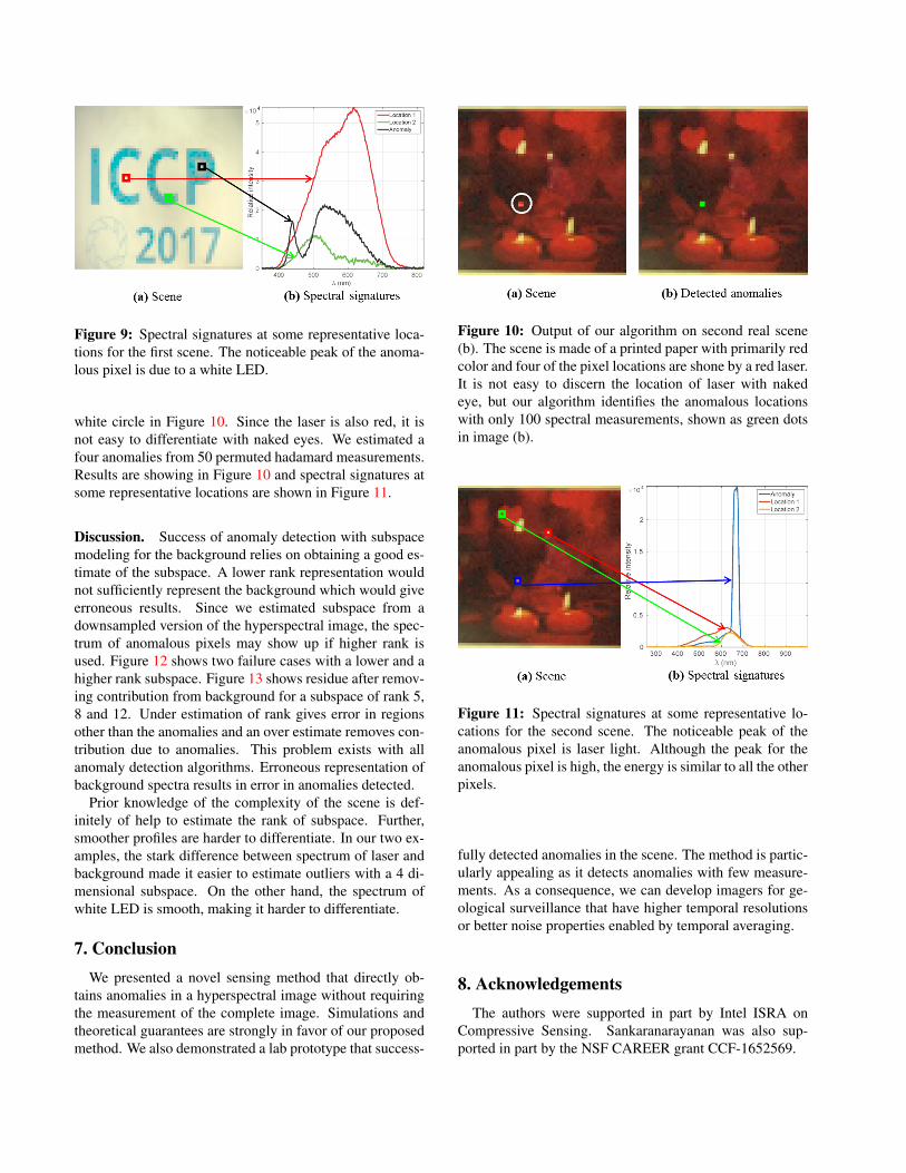
Figure 9: Spectral signatures at some representative loca-tions for the first scene. The noticeable peak of the anoma-lous pixel is due to a white LED.

white circle in Figure 10. Since the laser is also red, it isnot easy to differentiate with naked eyes. We estimated afour anomalies from 50 permuted hadamard measurements.Results are showing in Figure 10 and spectral signatures atsome representative locations are shown in Figure 11.

Discussion. Success of anomaly detection with subspacemodeling for the background relies on obtaining a good es-timate of the subspace. A lower rank representation wouldnot sufficiently represent the background which would giveerroneous results. Since we estimated subspace from adownsampled version of the hyperspectral image, the spec-trum of anomalous pixels may show up if higher rank isused. Figure 12 shows two failure cases with a lower and ahigher rank subspace. Figure 13 shows residue after remov-ing contribution from background for a subspace of rank 5,8 and 12. Under estimation of rank gives error in regionsother than the anomalies and an over estimate removes con-tribution due to anomalies. This problem exists with allanomaly detection algorithms. Erroneous representation ofbackground spectra results in error in anomalies detected.

Prior knowledge of the complexity of the scene is def-initely of help to estimate the rank of subspace. Further,smoother profiles are harder to differentiate. In our two ex-amples, the stark difference between spectrum of laser andbackground made it easier to estimate outliers with a 4 di-mensional subspace. On the other hand, the spectrum ofwhite LED is smooth, making it harder to differentiate.

7. ConclusionWe presented a novel sensing method that directly ob-

tains anomalies in a hyperspectral image without requiringthe measurement of the complete image. Simulations andtheoretical guarantees are strongly in favor of our proposedmethod. We also demonstrated a lab prototype that success-

Figure 10: Output of our algorithm on second real scene(b). The scene is made of a printed paper with primarily redcolor and four of the pixel locations are shone by a red laser.It is not easy to discern the location of laser with nakedeye, but our algorithm identifies the anomalous locationswith only 100 spectral measurements, shown as green dotsin image (b).

Figure 11: Spectral signatures at some representative lo-cations for the second scene. The noticeable peak of theanomalous pixel is laser light. Although the peak for theanomalous pixel is high, the energy is similar to all the otherpixels.

fully detected anomalies in the scene. The method is partic-ularly appealing as it detects anomalies with few measure-ments. As a consequence, we can develop imagers for ge-ological surveillance that have higher temporal resolutionsor better noise properties enabled by temporal averaging.

8. AcknowledgementsThe authors were supported in part by Intel ISRA on

Compressive Sensing. Sankaranarayanan was also sup-ported in part by the NSF CAREER grant CCF-1652569.

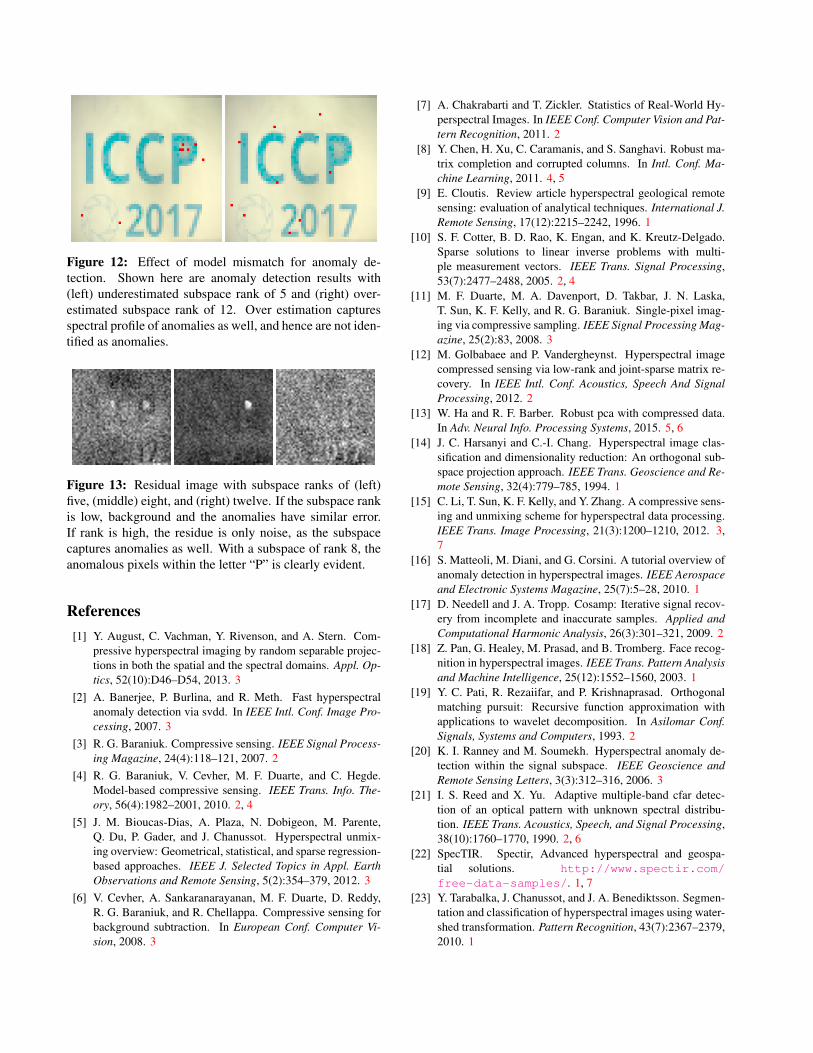
Figure 12: Effect of model mismatch for anomaly de-tection. Shown here are anomaly detection results with(left) underestimated subspace rank of 5 and (right) over-estimated subspace rank of 12. Over estimation capturesspectral profile of anomalies as well, and hence are not iden-tified as anomalies.

Figure 13: Residual image with subspace ranks of (left)five, (middle) eight, and (right) twelve. If the subspace rankis low, background and the anomalies have similar error.If rank is high, the residue is only noise, as the subspacecaptures anomalies as well. With a subspace of rank 8, theanomalous pixels within the letter “P” is clearly evident.

References[1] Y. August, C. Vachman, Y. Rivenson, and A. Stern. Com-

pressive hyperspectral imaging by random separable projec-tions in both the spatial and the spectral domains. Appl. Op-tics, 52(10):D46–D54, 2013. 3

[2] A. Banerjee, P. Burlina, and R. Meth. Fast hyperspectralanomaly detection via svdd. In IEEE Intl. Conf. Image Pro-cessing, 2007. 3

[3] R. G. Baraniuk. Compressive sensing. IEEE Signal Process-ing Magazine, 24(4):118–121, 2007. 2

[4] R. G. Baraniuk, V. Cevher, M. F. Duarte, and C. Hegde.Model-based compressive sensing. IEEE Trans. Info. The-ory, 56(4):1982–2001, 2010. 2, 4

[5] J. M. Bioucas-Dias, A. Plaza, N. Dobigeon, M. Parente,Q. Du, P. Gader, and J. Chanussot. Hyperspectral unmix-ing overview: Geometrical, statistical, and sparse regression-based approaches. IEEE J. Selected Topics in Appl. EarthObservations and Remote Sensing, 5(2):354–379, 2012. 3

[6] V. Cevher, A. Sankaranarayanan, M. F. Duarte, D. Reddy,R. G. Baraniuk, and R. Chellappa. Compressive sensing forbackground subtraction. In European Conf. Computer Vi-sion, 2008. 3

[7] A. Chakrabarti and T. Zickler. Statistics of Real-World Hy-perspectral Images. In IEEE Conf. Computer Vision and Pat-tern Recognition, 2011. 2

[8] Y. Chen, H. Xu, C. Caramanis, and S. Sanghavi. Robust ma-trix completion and corrupted columns. In Intl. Conf. Ma-chine Learning, 2011. 4, 5

[9] E. Cloutis. Review article hyperspectral geological remotesensing: evaluation of analytical techniques. International J.Remote Sensing, 17(12):2215–2242, 1996. 1

[10] S. F. Cotter, B. D. Rao, K. Engan, and K. Kreutz-Delgado.Sparse solutions to linear inverse problems with multi-ple measurement vectors. IEEE Trans. Signal Processing,53(7):2477–2488, 2005. 2, 4

[11] M. F. Duarte, M. A. Davenport, D. Takbar, J. N. Laska,T. Sun, K. F. Kelly, and R. G. Baraniuk. Single-pixel imag-ing via compressive sampling. IEEE Signal Processing Mag-azine, 25(2):83, 2008. 3

[12] M. Golbabaee and P. Vandergheynst. Hyperspectral imagecompressed sensing via low-rank and joint-sparse matrix re-covery. In IEEE Intl. Conf. Acoustics, Speech And SignalProcessing, 2012. 2

[13] W. Ha and R. F. Barber. Robust pca with compressed data.In Adv. Neural Info. Processing Systems, 2015. 5, 6

[14] J. C. Harsanyi and C.-I. Chang. Hyperspectral image clas-sification and dimensionality reduction: An orthogonal sub-space projection approach. IEEE Trans. Geoscience and Re-mote Sensing, 32(4):779–785, 1994. 1

[15] C. Li, T. Sun, K. F. Kelly, and Y. Zhang. A compressive sens-ing and unmixing scheme for hyperspectral data processing.IEEE Trans. Image Processing, 21(3):1200–1210, 2012. 3,7

[16] S. Matteoli, M. Diani, and G. Corsini. A tutorial overview ofanomaly detection in hyperspectral images. IEEE Aerospaceand Electronic Systems Magazine, 25(7):5–28, 2010. 1

[17] D. Needell and J. A. Tropp. Cosamp: Iterative signal recov-ery from incomplete and inaccurate samples. Applied andComputational Harmonic Analysis, 26(3):301–321, 2009. 2

[18] Z. Pan, G. Healey, M. Prasad, and B. Tromberg. Face recog-nition in hyperspectral images. IEEE Trans. Pattern Analysisand Machine Intelligence, 25(12):1552–1560, 2003. 1

[19] Y. C. Pati, R. Rezaiifar, and P. Krishnaprasad. Orthogonalmatching pursuit: Recursive function approximation withapplications to wavelet decomposition. In Asilomar Conf.Signals, Systems and Computers, 1993. 2

[20] K. I. Ranney and M. Soumekh. Hyperspectral anomaly de-tection within the signal subspace. IEEE Geoscience andRemote Sensing Letters, 3(3):312–316, 2006. 3

[21] I. S. Reed and X. Yu. Adaptive multiple-band cfar detec-tion of an optical pattern with unknown spectral distribu-tion. IEEE Trans. Acoustics, Speech, and Signal Processing,38(10):1760–1770, 1990. 2, 6

[22] SpecTIR. Spectir, Advanced hyperspectral and geospa-tial solutions. http://www.spectir.com/free-data-samples/. 1, 7

[23] Y. Tarabalka, J. Chanussot, and J. A. Benediktsson. Segmen-tation and classification of hyperspectral images using water-shed transformation. Pattern Recognition, 43(7):2367–2379,2010. 1

[24] J. A. Tropp. Just relax: Convex programming methods foridentifying sparse signals in noise. IEEE Trans. Info. Theory,52(3):1030–1051, 2006. 2

[25] F. Vagni. Survey of hyperspectral and multispectral imagingtechnologies. DTIC Document, 2007. 3

[26] A. Wagadarikar, R. John, R. Willett, and D. Brady. Singledisperser design for coded aperture snapshot spectral imag-ing. Appl. Optics, 47(10):B44–B51, 2008. 3

[27] A. E. Waters, A. C. Sankaranarayanan, and R. Baraniuk.Sparcs: Recovering low-rank and sparse matrices from com-pressive measurements. In Adv. Neural Info. Processing Sys-tems, 2011. 2, 5

[28] J. Wright, A. Ganesh, S. Rao, Y. Peng, and Y. Ma. Robustprincipal component analysis: Exact recovery of corruptedlow-rank matrices via convex optimization. In Adv. NeuralInfo. Processing Systems, 2009. 3, 5

[29] Y.-Q. Zhao and J. Yang. Hyperspectral image denoising viasparse representation and low-rank constraint. IEEE Trans.Geoscience and Remote Sensing, 53(1):296–308, 2015. 2