Commodity price beliefs, financial frictions and business ... · Commodity Price Beliefs, Financial...
38
Commodity Price Beliefs, Financial Frictions and Business Cycles Jesús Bejarano Franz Hamann Enrique G. Mendoza 1 Diego Rodríguez Preliminary Work Closing Conference - BIS CCA Research Network on “The commodity cycle: macroeconomic and financial stability implications” Mexico City, August 18-19 2016 1 University of Pennsylvania, NBER and PIER. Remaining authors are at Banco de la República.
Transcript of Commodity price beliefs, financial frictions and business ... · Commodity Price Beliefs, Financial...

Commodity Price Beliefs, Financial Frictions andBusiness Cycles
Jesús Bejarano Franz Hamann Enrique G. Mendoza1 Diego Rodríguez
Preliminary Work
Closing Conference - BIS CCA Research Network on “The commoditycycle: macroeconomic and financial stability implications”
Mexico City, August 18-19 2016
1University of Pennsylvania, NBER and PIER. Remaining authors are at Banco de la República.

Commodity cycle challenges macro and financial stability
I Commodity price volatility has affected commodity-exportersmacro performance, through now well-known changes inincentives to borrow/lend in presence of financial frictions2
I This kind of risk to oil exporting economies is usuallyuninsured in international financial markets and the macro andfinancial adjustment works through the real exchange rate(RER) and net foreign financial assets (NFA)
I Furthermore, with financial frictions (collateral constraints)there is a pecuniary externality: agents do not internalize whenthey borrow in “good times” that high leverage causes collapsein collateral values and credit crunch in “bad times” (Fisheriandeflation)
2See Mendoza (1991;95), Uribe & Yue (2006), Bianchi, Boz & Mendoza(2012), Bianchi & Mendoza (2015)]

Uncertainty reflected in spot prices as well as in futures
0
20
40
60
80
100
120
140
160
00-M
1
00-M
7
01-M
1
01-M
7
02-M
1
02-M
7
03-M
1
03-M
7
04-M
1
04-M
7
05-M
1
05-M
7
06-M
1
06-M
7
07-M
1
07-M
7
08-M
1
08-M
7
09-M
1
09-M
7
10-M
1
10-M
7
11-M
1
11-M
7
12-M
1
12-M
7
13-M
1
13-M
7
14-M
1
14-M
7
15-M
1
15-M
7
16-M
1
16-M
7
WTI
Oil
Pric
e (U
SD p
er B
arre
l)
Month
Spot Jul-14 Aug-14 Sep-14 Jan-15 Feb-15 Mar-15
2014-Q3
2015-Q1

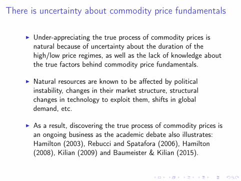
There is uncertainty about commodity price fundamentals
I Under-appreciating the true process of commodity prices isnatural because of uncertainty about the duration of thehigh/low price regimes, as well as the lack of knowledge aboutthe true factors behind commodity price fundamentals.
I Natural resources are known to be affected by politicalinstability, changes in their market structure, structuralchanges in technology to exploit them, shifts in globaldemand, etc.
I As a result, discovering the true process of commodity prices isan ongoing business as the academic debate also illustrates:Hamilton (2003), Rebucci and Spatafora (2006), Hamilton(2008), Kilian (2009) and Baumeister & Kilian (2015).

Commodity price beliefs interact with financial frictionsI When there is uncertainty about commodity price
fundamentals, optimistic beliefs or good news aboutcommodity prices strengthen incentives to borrow “today” andincrease expected future borrowing capacity3 but also...
I optimistic beliefs change the incentives to exploit naturalresources (real assets) affecting reserves and extraction of thecommodity
I ... and if followed by disappointing price outcomes, theprobability of a financial crisis rises because of higher leverageand the endogenous cutback in commodity extraction.
I In this paper, discrepancies between initial expectations aboutprices and actual and posterior expected prices can be animportant source of macro and financial instability because itaffects non-trivially both households and firms.
3Cogley and Sargent (2008), Boz (2009) and Boz, Daude and Durdu (2009)

A model of a commodity exporting economy...I Time, t = 0, 1, 2, . . . , economy with y
T , yN and a stock ofcommodity s̄ > 0, all in fixed supply. Every t there iss
t
2 [0, s̄] extracts x
t
2 [0, st
] and discovers d � 0:
s
t+1 = s
t
� x
t
+ d .
I Commodity price p
t
has a “true” TPM, Q (pt+1, pt), unknown
to agents. The value of a competitive firm with perfect accessto financial markets is:
v(st
, pt
) = maxx2[0,s
t
]
n
p
t
x
t
� e(st
, xt
) + R
�1EB
t
[v (st+1, pt+1)]
o
E
B
t
is conditional on the agents beliefs with the informationavailable up to t. Rational expectations: E
t
.
I Inter-temporal optimality condition:
p
t
� e
x
(st
, xt
) =EB
t
[pt+1 � e
x
(st+1, xt+1)� e
s
(st+1, xt+1)]
R
.

... with “liability dollarization”
Let x̃ be the firm’s optimal extraction. HH maximize:
EB
0
" 1X
t=0
�t
c
1��t
1 � �
#
c
t
=
a
⇣
c
T
t
⌘�µ+ (1 � a)
⇣
c
N
t
⌘�µ�� 1
µ
, a > 0, µ � �1
subject to
c
T
t
+p
N
t
c
N
t
= y
T+⌧⇡⇡ (pt
, st
)+⌧E
e(st
, x̃ (pt
, st
))+p
N
t
y
N�b
t+1+Rb
t
with ⇡ ⌘ p
t
x̃
t
� e (st
, x̃t
) and ⌧⇡ ⌘ ⌧S
p
t
x̃
t
�⌧E
e(st
,x̃t
)⇡t
and
b
t+1 � ��⇣
y
T + ⌧⇡⇡ (pt
, st
) + ⌧E
e(st
, x̃ (pt
, st
)) + p
N
t
y
N
⌘
.

Rational expectations perfect information equilibrium
The recursive representation of REPI equilibrium conditions are:
p
N =
✓
1 � a
a
◆
c
T
y
N
�1+µ
c
�� = �REt
h
�
c
0���i
+ �
b
0 = y
T + ⌧S
px̃ (p, s)� c
T + Rb
b
0 � ��⇣
y
T + ⌧S
px̃ (p, s) + p
N
y
N
⌘

Equilibrium under Bayesian learning about commodity prices
I Follow Boz and Mendoza (2009) two-stage solution strategy:1. Bayesian learning. Take a history of price realizations observed
up to date t, pt = (pt
, pt�1, pt�2, . . . , p1) and generate a
sequence of posterior density functions�
f
�
Q
B | pt�
T
t=1 overT periods. Each f is a probability distribution over possibleQ
B ’s. The date t = 0 priors depend on the assumed amountof agents prior knowledge.
2. The problem can be divided into a sequence of AUoptimization problems (AUOP) for t = 1, 2, . . . ,T , eachconditional on E
t
⇥
q
B
hh
⇤
and Et
⇥
q
B
ll
⇤
, where the time indexesidentify the date of the beliefs that match the correspondingAUOP. So, we find a sequence of equilibrium policy functionsfor {x
t
}Tt=1 and {b0
t
}Tt=1, one for each set of beliefs at each
date t = 1, 2, . . . ,T .

Anticipated utility optimal problem
The solution to AUOP at date t is given by x̃
t
(s, p) which solves
v
t
(s, p) = maxx2X
n
[px � e(s, x)] + R
�1EB
t
⇥
v
t
�
s � x + d , p0�⇤
o
,
the policies b
0t
(b, s, p), ct
(b, s, p), cTt
(b, s, p), cNt
(b, s, p),�t
(b, s, p) and a pricing function p
N
t
(b, s, p) that satisfy HHoptimality as well as the MCC for T and NT sectors:
p
N
t
(b, s, p) =
✓
1 � a
a
◆
c
T
t
(b, s, p)
y
N
�1+µ
c
t
(b, s, p)�� = �REB
t
⇥
c
t+1 (b, s, p)��⇤+ �
t
(b, s, p)
b
0t
(b, s, p) = y
T + ⌧S
px̃
t
(s, p)� c
T
t
(b, s, p) + Rb
b
0t
(b, s, p) � �⇣
y
T + ⌧S
px̃
t
(s, p) + p
N
t
(b, s, p) yN⌘

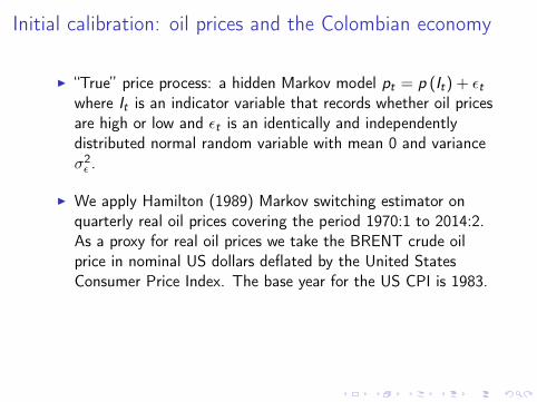
Initial calibration: oil prices and the Colombian economy
I “True” price process: a hidden Markov model pt
= p (It
) + ✏t
where I
t
is an indicator variable that records whether oil pricesare high or low and ✏
t
is an identically and independentlydistributed normal random variable with mean 0 and variance�2✏ .
I We apply Hamilton (1989) Markov switching estimator onquarterly real oil prices covering the period 1970:1 to 2014:2.As a proxy for real oil prices we take the BRENT crude oilprice in nominal US dollars deflated by the United StatesConsumer Price Index. The base year for the US CPI is 1983.
I Take the model ergodic moments under REPI to match bothaggregate and sectoral (oil) Colombian data.

Debt distribution from low to high commodity prices
In t = 1, pt
= p
h
and then for t = 2, . . . , 7 p
t
= p
l
.
0 0.2 0.4 0.6 0.8 1 1.2 1.4 1.60
0.5
1
1.5
2
2.5
3
3.5
137RE

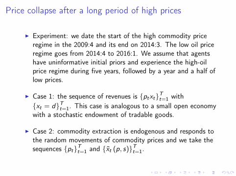
Price collapse after a long period of high prices
I Experiment: we date the start of the high commodity priceregime in the 2009:4 and its end on 2014:3. The low oil priceregime goes from 2014:4 to 2016:1. We assume that agentshave uninformative initial priors and experience the high-oilprice regime during five years, followed by a year and a half oflow prices.
I Case 1: the sequence of revenues is {pt
x
t
}Tt=1 with
{xt
= d}Tt=1. This case is analogous to a small open economy
with a stochastic endowment of tradable goods.
I Case 2: commodity extraction is endogenous and responds tothe random movements of commodity prices and we take thesequences {p
t
}Tt=1 and {x̃
t
(p, s)}Tt=1.
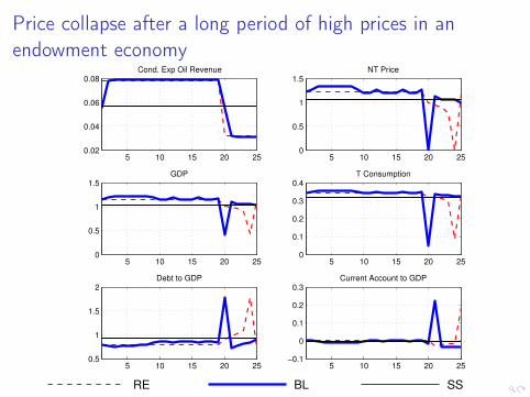
Price collapse after a long period of high prices in anendowment economy
5 10 15 20 250.02
0.04
0.06
0.08
Cond. Exp Oil Revenue
RE BL SS
5 10 15 20 250
0.5
1
1.5
NT Price
5 10 15 20 250
0.5
1
1.5
GDP
5 10 15 20 250
0.1
0.2
0.3
0.4
T Consumption
5 10 15 20 250.5
1
1.5
2
Debt to GDP
5 10 15 20 25−0.1
0
0.1
0.2
0.3
Current Account to GDP
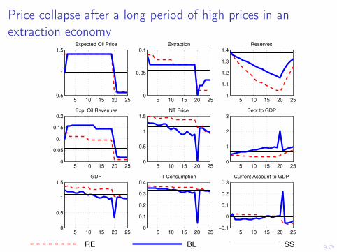
Price collapse after a long period of high prices in anextraction economy
5 10 15 20 250.5
1
1.5
Expected Oil Price
RE BL SS
5 10 15 20 250
0.05
0.1
Extraction
5 10 15 20 251
1.1
1.2
1.3
1.4
Reserves
5 10 15 20 250
0.05
0.1
0.15
0.2
Exp. Oil Revenues
5 10 15 20 250
0.5
1
1.5
NT Price
5 10 15 20 250
1
2
3
Debt to GDP
5 10 15 20 250
0.5
1
1.5
GDP
5 10 15 20 250
0.1
0.2
0.3
0.4
T Consumption
5 10 15 20 25−0.1
0
0.1
0.2
0.3
Current Account to GDP

Final Remarks
I We presented a framework to analyze the interaction betweenuncertainty about commodity price fundamentals and financialfrictions.
I Model of natural resource extraction, incomplete financialmarkets and endogenous borrowing constraints capture macrodynamics (calibrated to Colombia and its oil sector)
I We showed how discrepancies between initial expectationsabout prices and actual and posterior expected prices can bean important source of macro and financial instability becauseit affects non-trivially both households and firms.
I Work in progress:I Analyze the quantitative effects of alternative beliefsI Shocks to R may be additional sources of uncertaintyI Oil ownership and operations may matterI Financing extraction operations
Sources of information
I Oil reserves, oil production (thousand barrels per day): US EnergyInformation Administration dataset (EIA). Annual data from 1980 to 2013
I Brent spot oil price (USD per barrel): US Energy InformationAdministration dataset (EIA). Annual data from 1980 to 2013.
I Total public debt to GDP: World Development Indicators tables (WDI)and World Economic Outlook database (WEO). Annual data from 1979to 2010.
I Net Foreign Assets: Lane and Milesi-Ferreti (2007). Annual data from1970 to 2011.
I Default data: Borensztein and Panizza (2006). Annual data from 1979 to2010.
I GDP: World Economic Outlook database (WEO). Annual data from 1979to 2010.

Oil price upswings and downswings
Downswings Upswings
Period Number of Months Period Number of Months
NOV 75 - OCT 78 36 NOV 78 - JAN 81 27
FEB 81 - JUL 86 66 AUG 86 - JUL 87 12
AUG 87 - NOV 88 16 DEC 88 - OCT 90 23
NOV 90 - DEC 93 38 JAN 94 - OCT 96 34
NOV 96 - DEC 98 26 JAN 99 - SEP 00 21
OCT 00 - DEC 01 15 JAN 02 - JUL 08 79
AUG 08 - MAY 10 22
TOTAL 219 TOTAL 196

Oil price swings and macro performance of net oil exporters
Rea
lG
DP
Gro
wth
Rat
e(p
erce
nta
gepoi
nts
)
0
0.5
1
1.5
2
2.5
3
3.5
4Real GDP Growth Rate (percentage points)
Upswing Downswing
Curr
entA
ccou
nt(p
erce
ntof
GD
P)
-1.5
-1
-0.5
0
0.5
1Current Account (percent of GDP)
Upswing Downswing
Oil
Pro
duct
ion
Gro
wth
Rat
e
0
0.2
0.4
0.6
0.8
1
1.2
1.4
1.6
1.8
2Oil Production Growth Rate
Upswing Downswing
Chan
gein
Net
For
eign
Ass
ets(p
erce
ntof
GD
P)
-1
-0.5
0
0.5
1
1.5
2
2.5Change in Net Foreign Assets (percent of GDP)
Upswing Downswing
4
4Each bar is calculated with the same methodology of figure 4.4 of the World Economic Outlook of
April of 2012. For default events the average number of default events is calculated.

New Title
I Item 1I item aI item b
I Item 2I item aI item b

New Title
I Item 1I item aI item b
I Item 2I item aI item b