PAPER

Coarse-graining the dynamics of networkevolution: the rise and fall of a networked societyTo cite this article: Andreas C Tsoumanis et al 2012 New J. Phys. 14 083037

 

View the article online for updates and enhancements.

You may also likePreface-

SciDAC 2009Michael Strayer

-

Where were you when the sun went out?-

Recent citationsEquation-free analysis of agent-basedmodels and systematic parameterdeterminationSpencer A. Thomas et al

-

Coarse-Graining and Simplification of theDynamics Seen in Bursting NeuronsA. Ben-Tal and I. G. Kevrekidis

-

Modeling epidemics on adaptively evolvingnetworks: A data-mining perspectiveAssimakis A Kattis et al

-

This content was downloaded from IP address 61.253.62.88 on 20/12/2021 at 14:29

T h e o p e n – a c c e s s j o u r n a l f o r p h y s i c s

New Journal of Physics

Coarse-graining the dynamics of network evolution:the rise and fall of a networked society

Andreas C Tsoumanis1, Karthikeyan Rajendran1,Constantinos I Siettos2 and Ioannis G Kevrekidis1,3,4

1 Department of Chemical and Biological Engineering, Princeton University,Princeton, NJ, USA2 School of Applied Mathematics and Physical Sciences, NTUA, Athens,Greece3 Program in Applied and Computational Mathematics, Princeton University,Princeton, NJ, USAE-mail: yannis@princeton.edu

New Journal of Physics 14 (2012) 083037 (17pp)Received 18 February 2012Published 29 August 2012Online at http://www.njp.org/doi:10.1088/1367-2630/14/8/083037

Abstract. We explore a systematic approach to studying the dynamicsof evolving networks at a coarse-grained, system level. We emphasize theimportance of finding good observables (network properties) in terms ofwhich coarse-grained models can be developed. We illustrate our approachthrough a particular social network model: the ‘rise and fall’ of a networkedsociety (Marsili M et al 2004 Proc. Natl Acad. Sci. USA 101 1439). Weimplement our low-dimensional description computationally using the equation-free approach and show how it can be used to (i) accelerate simulations and (ii)extract system-level stability/bifurcation information from the detailed dynamicmodel. We discuss other system-level tasks that can be enabled through such acomputer-assisted coarse-graining approach.

4 Author to whom any correspondence should be addressed.

New Journal of Physics 14 (2012) 0830371367-2630/12/083037+17$33.00 © IOP Publishing Ltd and Deutsche Physikalische Gesellschaft

2

Contents

1. Introduction 22. An illustrative case: the rise and fall of a networked society 33. Selecting an appropriate low-dimensional description 44. A coarse-grained model 7

4.1. Our lifting operator . . . . . . . . . . . . . . . . . . . . . . . . . . . . . . . . 95. Computational results and discussion 106. Conclusions 13Acknowledgments 15Appendix. A simple singularly perturbed system of ordinary differential equations 15References 16

1. Introduction

The Erdos–Renyi random graph model [2], dating back to 1959, constitutes a landmark in thestudy of graphs. There has been renewed interest in networks (or graphs) in recent years with aspecific focus on complex emergent dynamics, spurred by discoveries such as power-law degreedistributions [3, 4], small world behavior [5] and so on. Dynamic network evolution modelshave been developed with an eye to constructing networks with specific structures/statisticalproperties; an example is the preferential attachment mechanism [6], proposed as a source ofscale-free structure in evolving networks. Evolutionary network models are especially popular(and relevant) in the social sciences [7–11]. The focus in many of these models is on thecorrespondence between local mechanisms (rules) of network formation and the resulting large-scale ‘system-level’ network structure and dynamics.

In this paper, we explore a systematic approach to the computer-assisted study of suchmodels at the macroscopic, coarse-grained, system level as opposed to the detailed, node-level,microscopic level. The basic idea is to estimate the information necessary for coarse-grainedcomputations on the fly, using short bursts of appropriately designed detailed simulations. Basedon the selection of suitable coarse variables (observables), this equation-free approach [12, 13]facilitates efficient computation at the coarse-grained level. Accelerating coarse-grainedevolution computations and/or enabling additional modeling tasks such as coarse fixedpoint/bifurcation/stability computations can significantly enhance our understanding of thesystem behavior at the macroscopic level, even when an explicit coarse-grained model is notavailable. The approach may also help pinpoint collective network properties that are crucial inthe evolution process (and could thus be used as coarse variables). The main aim of this paperis to demonstrate how our modeling approach to complex systems dynamics has to be modifiedand extended in order to be usable in problems involving network evolution. We will focus ona number of issues arising in this new context, such as finding the number of slow variables,constructing networks consistent with them and so on.

The paper is structured as follows. In the next section, we briefly describe an illustrativenetwork evolution model introduced by Marsili et al [1]. We then discuss certain issues thatarise in coarse variable selection, and our chosen coarse-graining approach. The results of the

New Journal of Physics 14 (2012) 083037 (http://www.njp.org/)

3

computational implementation of this approach are presented, and we conclude the paper witha discussion of the scope and applicability of our approach, as well as certain important openissues in the selection of coarse variables for general network evolution problems.

2. An illustrative case: the rise and fall of a networked society

We revisit the model of the rise and fall of a networked society [1] presented by Marsiliet al to illustrate our approach. Their model exhibits complex emergent phenomena arising fromsimple evolution rules; a brief description of these rules follows: consider a (social) networkconsisting of n agents (entities) involved in bilateral interactions. The network is representedby N = (V, E), where V is the set of vertices or nodes (agents) and E is the set of edges orlinks, indicating interactions between agents. In any time interval [t, t + dt), the model evolvesas follows:

1. Any existing edge (i, j) ∈ E is removed with probability λ dt .

2. With independent probability η dt , every agent i can form a link with (become a neighborof) a randomly chosen agent j 6= i . Nothing occurs if agent i is already a neighbor of (isconnected with) agent j .

3. With independent probability ξdt , every agent i is allowed to ask a neighbor j (randomlychosen) to introduce him/her to a randomly chosen neighbor of j , say agent k. If agent iis not already connected to agent k a new edge is formed between i and k. Nothing occursif agent i is already a neighbor of (is connected with) agent k.

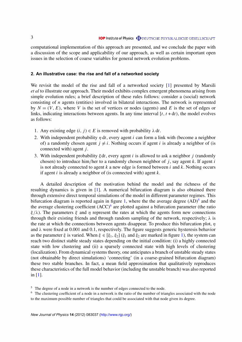
A detailed description of the motivation behind the model and the richness of theresulting dynamics is given in [1]. A numerical bifurcation diagram is also obtained therethrough extensive direct temporal simulations of the model in different parameter regimes. Thisbifurcation diagram is reported again in figure 1, where the the average degree (AD)5 and thethe average clustering coefficient (ACC)6 are plotted against a bifurcation parameter (the ratioξ/λ). The parameters ξ and η represent the rates at which the agents form new connectionsthrough their existing friends and through random sampling of the network, respectively; λ isthe rate at which the connections between agents disappear. To produce this bifurcation plot, η

and λ were fixed at 0.001 and 0.1, respectively. The figure suggests generic hysteresis behavioras the parameter ξ is varied. When ξ ∈ [ξ1, ξ2] (ξ1 and ξ2 are marked in figure 1), the system canreach two distinct stable steady states depending on the initial condition: (i) a highly connectedstate with low clustering and (ii) a sparsely connected state with high levels of clustering(localization). From dynamical systems theory, one anticipates a branch of unstable steady states(not obtainable by direct simulations) ‘connecting’ (in a coarse-grained bifurcation diagram)these two stable branches. In fact, a mean field approximation that qualitatively reproducesthese characteristics of the full model behavior (including the unstable branch) was also reportedin [1].

5 The degree of a node in a network is the number of edges connected to the node.6 The clustering coefficient of a node in a network is the ratio of the number of triangles associated with the nodeto the maximum possible number of triangles that could be associated with that node given its degree.

New Journal of Physics 14 (2012) 083037 (http://www.njp.org/)

4

Figure 1. Bifurcation diagram obtained using direct temporal simulations,reproduced from [1] with permission (copyright 2004 National Academy ofSciences, USA). Steady state values of average degree (AD), average clusteringcoefficient (ACC) are plotted against the ratio of parameters, ξ/λ. η and λ valueswere fixed at 0.001 and 0.1, respectively. Note the robustness of the results to thenetwork size.

3. Selecting an appropriate low-dimensional description

One of the crucial steps in developing a reduced, coarse-grained description of any complexsystem is the selection of suitable observables (coarse variables). We borrow simple principlesfrom dynamical systems to help us in this pursuit and to provide the rationale corroborating ourcoarse variable choices. In order for a system to exhibit low-dimensional behavior, one expectsa separation of time scales to prevail in the evolution of different variables in the system phasespace. The basic picture is that low-dimensional subspaces (slow manifolds, parameterizedby ‘slow’ variables) contain the long-term dynamics, while fast evolution in the transversedirections (in the ‘fast’ variables) quickly brings the system trajectories close to the (attracting)slow manifolds. Thus, the problem of selecting good coarse variables is translated to the problemof finding a set of variables that successfully parameterize the slow manifold(s), when such amanifold exists.

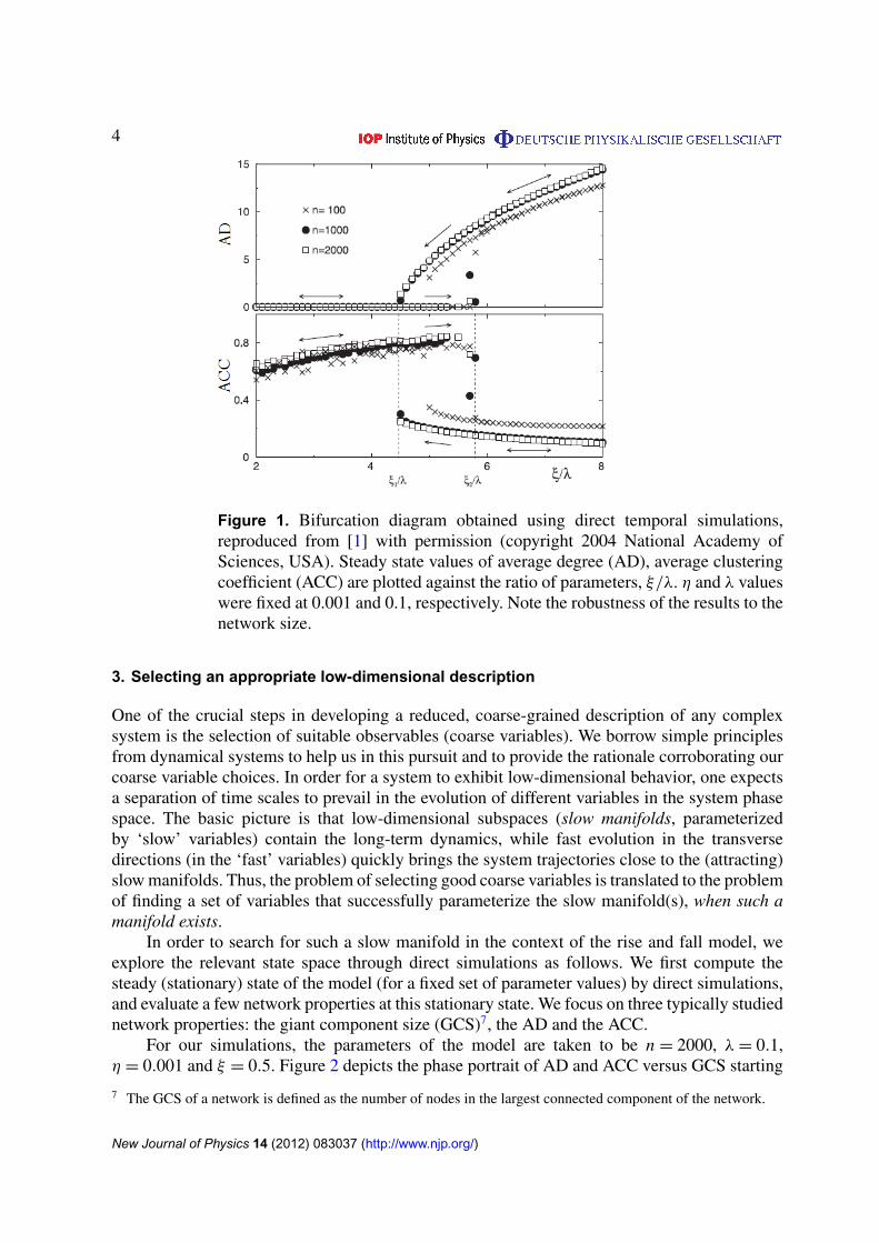
In order to search for such a slow manifold in the context of the rise and fall model, weexplore the relevant state space through direct simulations as follows. We first compute thesteady (stationary) state of the model (for a fixed set of parameter values) by direct simulations,and evaluate a few network properties at this stationary state. We focus on three typically studiednetwork properties: the giant component size (GCS)7, the AD and the ACC.

For our simulations, the parameters of the model are taken to be n = 2000, λ = 0.1,η = 0.001 and ξ = 0.5. Figure 2 depicts the phase portrait of AD and ACC versus GCS starting

7 The GCS of a network is defined as the number of nodes in the largest connected component of the network.

New Journal of Physics 14 (2012) 083037 (http://www.njp.org/)

5

Figure 2. Phase portrait in terms of giant component size (GCS) and AD (left)or ACC (right) showing transients from a variety of initial conditions. Fast (resp.slow) temporal evolution is indicated by a double (resp. a single) arrow.

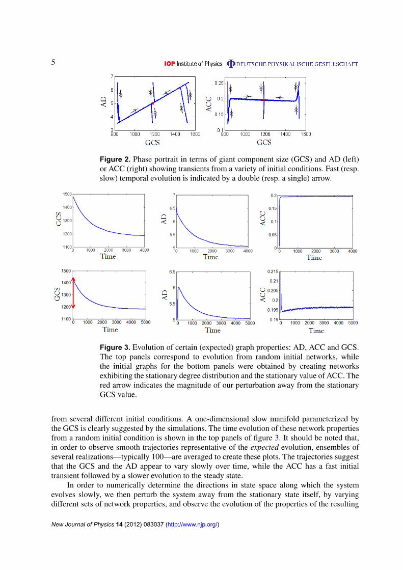
Figure 3. Evolution of certain (expected) graph properties: AD, ACC and GCS.The top panels correspond to evolution from random initial networks, whilethe initial graphs for the bottom panels were obtained by creating networksexhibiting the stationary degree distribution and the stationary value of ACC. Thered arrow indicates the magnitude of our perturbation away from the stationaryGCS value.

from several different initial conditions. A one-dimensional slow manifold parameterized bythe GCS is clearly suggested by the simulations. The time evolution of these network propertiesfrom a random initial condition is shown in the top panels of figure 3. It should be noted that,in order to observe smooth trajectories representative of the expected evolution, ensembles ofseveral realizations—typically 100—are averaged to create these plots. The trajectories suggestthat the GCS and the AD appear to vary slowly over time, while the ACC has a fast initialtransient followed by a slower evolution to the steady state.

In order to numerically determine the directions in state space along which the systemevolves slowly, we then perturb the system away from the stationary state itself, by varyingdifferent sets of network properties, and observe the evolution of the properties of the resulting

New Journal of Physics 14 (2012) 083037 (http://www.njp.org/)

6

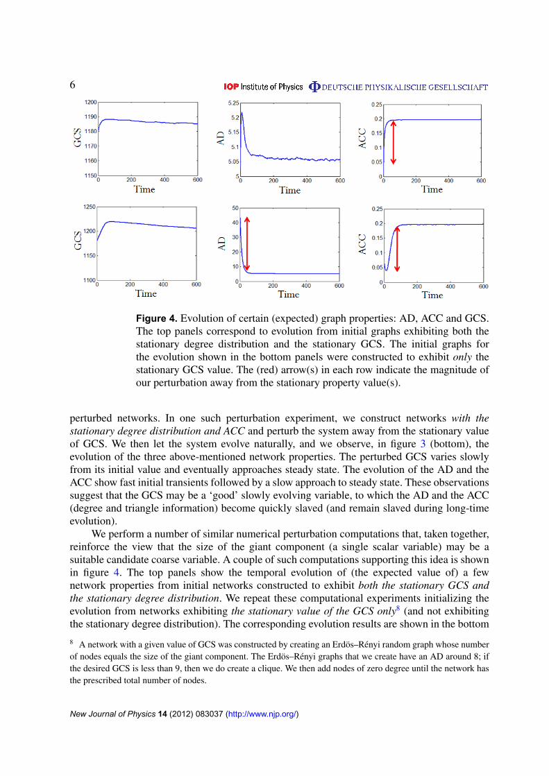
Figure 4. Evolution of certain (expected) graph properties: AD, ACC and GCS.The top panels correspond to evolution from initial graphs exhibiting both thestationary degree distribution and the stationary GCS. The initial graphs forthe evolution shown in the bottom panels were constructed to exhibit only thestationary GCS value. The (red) arrow(s) in each row indicate the magnitude ofour perturbation away from the stationary property value(s).

perturbed networks. In one such perturbation experiment, we construct networks with thestationary degree distribution and ACC and perturb the system away from the stationary valueof GCS. We then let the system evolve naturally, and we observe, in figure 3 (bottom), theevolution of the three above-mentioned network properties. The perturbed GCS varies slowlyfrom its initial value and eventually approaches steady state. The evolution of the AD and theACC show fast initial transients followed by a slow approach to steady state. These observationssuggest that the GCS may be a ‘good’ slowly evolving variable, to which the AD and the ACC(degree and triangle information) become quickly slaved (and remain slaved during long-timeevolution).

We perform a number of similar numerical perturbation computations that, taken together,reinforce the view that the size of the giant component (a single scalar variable) may be asuitable candidate coarse variable. A couple of such computations supporting this idea is shownin figure 4. The top panels show the temporal evolution of (the expected value of) a fewnetwork properties from initial networks constructed to exhibit both the stationary GCS andthe stationary degree distribution. We repeat these computational experiments initializing theevolution from networks exhibiting the stationary value of the GCS only8 (and not exhibitingthe stationary degree distribution). The corresponding evolution results are shown in the bottom

8 A network with a given value of GCS was constructed by creating an Erdos–Renyi random graph whose numberof nodes equals the size of the giant component. The Erdos–Renyi graphs that we create have an AD around 8; ifthe desired GCS is less than 9, then we do create a clique. We then add nodes of zero degree until the network hasthe prescribed total number of nodes.

New Journal of Physics 14 (2012) 083037 (http://www.njp.org/)

7

panels of figure 4. We find that, if we initialize with networks that exhibit the ‘correct’ stationaryvalue of the GCS, the AD will quickly evolve to the neighborhood of its stationary value—‘comedown’ on the slow manifold—and will then slowly approach it on the same time scale as theGCS does. This would suggest that the AD is a ‘fast variable’. By the same type of argument,figures 3 and 4 suggest that the ACC also is a fast variable and hence does not need to beexplicitly included in a model for the long-term evolution.

In both the cases shown in figure 4, the GCS itself has a fast initial evolution window thattakes it momentarily away from the steady state value and then it slowly evolves back towardsit (on the slow manifold). While the GCS is a good candidate coarse variable to parameterizethe slow manifold (and the long-term dynamics), these transients indicate that it is not a pureslow variable—its evolution appears to have initial fast as well as slow components. A clearillustration (and explanation) of this behavior and of the concept of a ‘pure’ slow variable in thecontext of a simple singularly perturbed problem can be found in the appendix. These dynamicsimply that initializing with a desired value of the GCS is not sufficient; additional care mustbe taken to find a network that exhibits this value but also lies close to the slow manifold(explained later below). If the variable was a pure slow one, then just a few simulation stepswould guarantee the latter property (lying close to the slow manifold; for a simple illustration,see the appendix).

4. A coarse-grained model

Once we have chosen suitable coarse variables, computations at the coarse-grained level arecarried out using the equation-free framework [12, 13]. This framework is used to acceleratesimulation and also to enable performing a number of additional tasks (such as fixed pointcomputation and stability analysis) at the coarse-grained level. In this approach, computationsinvolving the coarse variables are performed with the help of suitably defined operators whichtranslate between coarse and fine descriptions. Short bursts of fine scale simulation followed byobservation and post-processing of the results at the coarse scale enable on-demand estimationof numerical quantities (residuals, actions of Jacobians and time derivatives) required forcoarse numerics. The operator that transforms coarse variables into the detailed, fine variablesis called the lifting operator, L , while the operator that transforms fine variables back tocoarse variables is called the restriction operator, R. One can thus evolve the coarse variablesof a system forward in time for a given number of steps t by performing the followingoperations:

1. Lifting (L). Find a set of detailed variables (networks) consistent with the initial value(s) ofthe coarse variable(s) (here, the GCS).

2. Microscopic evolution. Evolve the fine variables (the nodes and edges of the networks) fora specified time t using the detailed, microscopic evolution rules of the system.

3. Restriction (R). Observe the fine variables, from the final stage(s) of the previous step, atthe coarse scale.

These steps constitute what is known as the coarse time-stepper, which acts as a substitutecode for the unavailable macroscopic evolution equations of the system. In terms of the liftingand restriction operators, the coarse time-stepper 8t can be written in terms of the fine scale

New Journal of Physics 14 (2012) 083037 (http://www.njp.org/)

8

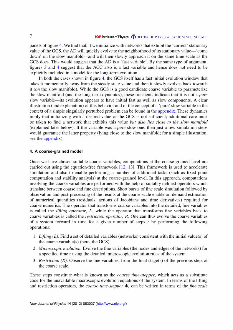
Figure 5. Schematic diagram of our lifting procedure for creating graphs with aspecified GCS which also lie close to the slow manifold. The process begins withthe network labeled 1 (see text).

evolution operator (φt ) as

8t(·) = R ◦ φt ◦ L(·). (1)

Using this coarse time-stepper in the form of a black-box subroutine, we can ‘wrap’ aroundit a number of different algorithms (initial value solvers, fixed point solvers, eigensolvers)that perform system-level tasks. In our present example, the microscopic description ofsystem evolution is the model itself, defined in terms of the network structure (fine variables,information about the edges between nodes), while the GCS is the single coarse variable. Hence,the restriction operation consists of simply evaluating the GCS of a given network. The liftingoperation, however, consists of constructing a network with a specified value of GCS; this byitself, however, is not sufficient for equation-free computations, as we need a network that hasthe specified GCS and lies on or close to the slow manifold.

We show a schematic diagram representing the state space of our dynamical system infigure 5. The x-axis represents our coarse variable, the GCS, while the y-axis represents thedirections corresponding to all other possible variations in the network that do not alter theGCS. The solid (blue) line denotes the slow manifold, which is drawn in a manner suggestinga good one-to-one correspondence to our chosen coarse variable (GCS). The vertical, dashed(black) line represents a family of graphs having the same (prescribed) GCS. Let us pick onegraph in this family denoted by the (green) point number 1 and use it as an initial condition inthe model we study. If the GCS were truly a slow variable, the system would ‘quickly’ evolve toa point on the manifold with a GCS very similar to the starting value. However, as we observedbefore, the GCS is not a pure slow variable: as the system dynamics quickly evolve from point1 to point 2, we do approach the slow manifold, yet our GCS has significantly changed. It istherefore important that our lifting operation constructs networks that not only conform to theprescribed GCS but also lie close to the slow manifold. In terms of our schematic caricature infigure 5, the vertical line corresponds to the required value of GCS and the lifting operation isrequired to produce a graph close to point D. The issue of initializing on the slow manifold is acrucial one in many scientific contexts that involve model reduction (e.g. in meteorology; [14]),and algorithms for accomplishing it in a dynamical systems context are the subject of currentresearch (see, e.g., [15, 16]).

New Journal of Physics 14 (2012) 083037 (http://www.njp.org/)

9

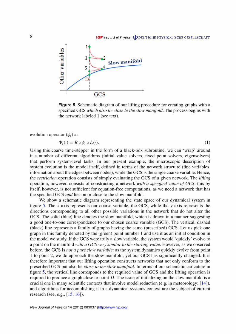
Figure 6. The graph evolution during our lifting operation is tracked throughplots of AD and ACC versus GCS. Here, the required value of GCS is 1120.The graph with this desired value of GCS and on the slow manifold (plottedas a green thin dotted line) is labeled as ‘D’. The lifting operator arrives at itthrough the intermediate graphs 1–5, in that order. The dashed (blue) lines denotethe evolution of the dynamical model: this is the ‘process step’. The solid (red)lines denote corrections for the change in GCS: this is the ‘adjustment step’. Thecombination of two such steps constitutes a single full iteration. Two such fulliterations are shown in this illustration.

4.1. Our lifting operator

We implement such a lifting operation beginning with a network that possesses the requiredvalue of GCS, by creating an Erdos–Renyi random graph9 whose number of nodes is equal tothe size of the giant component; we then add nodes of zero degree until the network has thecorrect number of total nodes. Let us denote this result by point 1 in figure 5. We then run themodel for a few (here, typically 70) time steps and obtain network 2, which lies close to the slowmanifold, but has a different value of GCS than required. We now appropriately add/removeenough nodes from this network 2 until the resulting network 3 has the required number ofnodes in its giant component. This adjustment step is illustrated as a straight line segment in theschematic diagram, for convenience (we do not control the other variables during the adjustmentstep). If we add nodes to the giant component, we assign them a degree sampled from the currentgiant component degree distribution. This can be done by randomly selecting a node in thecurrent giant component and using its degree as the degree of the added node. This node is thenconnected to as many nodes of the giant component as its degree. If we remove nodes from thegiant component, they become isolated nodes of degree 0. When removing nodes, one must ofcourse be careful not to break up the giant component. This is taken care of by first constructinga spanning tree of the giant component, and only removing the fringe nodes of degree 1 in thistree. All the edges connected to this node in the original graph are then finally removed. In thispaper, these lifting steps are repeated two or three times as necessary (2 → 3, 4 → 5, . . .) so that

9 Note that these initial graphs are essentially initial guesses for our lifting operator, which creates graphs havingthe specified value of GCS and lying close to the slow manifold. A good initial guess reduces the computationaleffort involved in finding such a graph. Thus, although we can successfully lift under a variety of differentreasonable initial conditions, computational efficiency does depend on the initial condition used.

New Journal of Physics 14 (2012) 083037 (http://www.njp.org/)

10

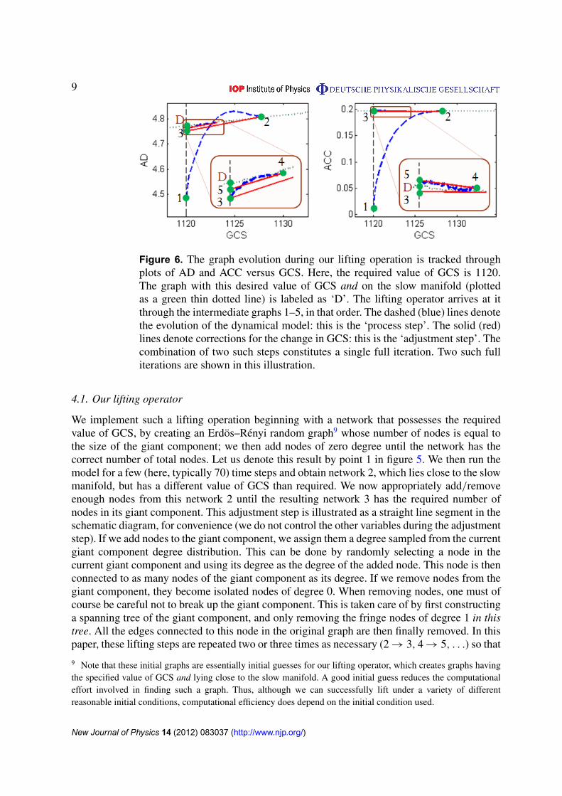
Figure 7. Trajectories of GCS observed by simulations from two different classesof initial conditions. The dashed (blue) curve corresponds to the case where theinitial condition is a random network created with the stationary values of theGCS and of the ACC as well as the stationary degree distribution. The solid (red)curve corresponds to initial networks created by our lifting procedure, exhibitingthe stationary GCS and lying on/close to the slow manifold.

we obtain a network close to the desired graph D in the schematic diagram. We also show anactual sample graph evolution during our lifting operation in figure 6. In this case, the requiredGCS is 1120. We start from an Erdos–Renyi random graph (AD around 4.5) and perform twoiterations of the lifting operation. As explained earlier, each iteration consists of a process step(blue dashed line) and an adjustment step (red solid line). The desired, ‘lifted’ graph is labeledas ‘D’; the lifting operator arrives at it through intermediate graphs in the sequence from 1 to 5.

We illustrate the effect of this lifting procedure by evolving the model from two differentinitial conditions. In the first case, we use a random network created to exhibit the stationaryvalues of the GCS, the degree distribution and the ACC. The evolution of GCS in this case,shown in figure 7 as a dashed line (blue), is reminiscent of the left panels of figure 4. Thus, itis clear that initializing with the stationary values of GCS, ACC and degree distribution is notsufficient to keep the system close to the slow dynamics; fast transients that take these variablesaway from their stationary values ensue.

In the second case, we use the lifting procedure just described above to create networksthat exhibit the stationary GCS value but also lie close to the slow manifold. Figure 7 showsthe evolution of the GCS when we run the model starting from these lifted networks as a solid(red) line. Now the GCS remains close to its stationary value, as desired. This suggests that ourlifting procedure is successful.

5. Computational results and discussion

We first validate our coarse-grained modeling by illustrating coarse projective integration ofthe (expected, averaged over many realizations) system dynamics; we then present coarsebifurcation computations. Let g denote the coarse variable, the GCS. We start with an ensembleof 2000 realizations of networks (each with n = 2000 nodes) exhibiting a specified initial valueof this GCS g0. g is evolved using the coarse time-stepper (equation (1)) for a few (here, 60)time steps. The GCS is observed from simulations and its time derivative is estimated from

New Journal of Physics 14 (2012) 083037 (http://www.njp.org/)

11

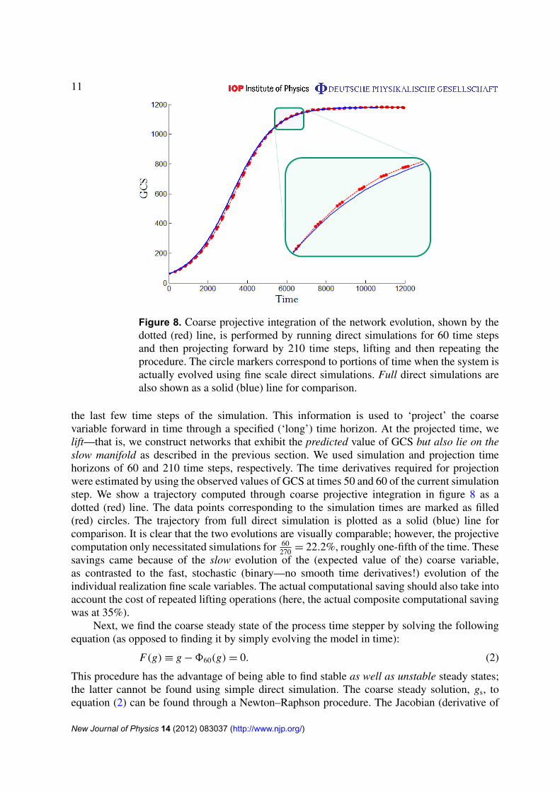
Figure 8. Coarse projective integration of the network evolution, shown by thedotted (red) line, is performed by running direct simulations for 60 time stepsand then projecting forward by 210 time steps, lifting and then repeating theprocedure. The circle markers correspond to portions of time when the system isactually evolved using fine scale direct simulations. Full direct simulations arealso shown as a solid (blue) line for comparison.

the last few time steps of the simulation. This information is used to ‘project’ the coarsevariable forward in time through a specified (‘long’) time horizon. At the projected time, welift—that is, we construct networks that exhibit the predicted value of GCS but also lie on theslow manifold as described in the previous section. We used simulation and projection timehorizons of 60 and 210 time steps, respectively. The time derivatives required for projectionwere estimated by using the observed values of GCS at times 50 and 60 of the current simulationstep. We show a trajectory computed through coarse projective integration in figure 8 as adotted (red) line. The data points corresponding to the simulation times are marked as filled(red) circles. The trajectory from full direct simulation is plotted as a solid (blue) line forcomparison. It is clear that the two evolutions are visually comparable; however, the projectivecomputation only necessitated simulations for 60

270 = 22.2%, roughly one-fifth of the time. Thesesavings came because of the slow evolution of the (expected value of the) coarse variable,as contrasted to the fast, stochastic (binary—no smooth time derivatives!) evolution of theindividual realization fine scale variables. The actual computational saving should also take intoaccount the cost of repeated lifting operations (here, the actual composite computational savingwas at 35%).

Next, we find the coarse steady state of the process time stepper by solving the followingequation (as opposed to finding it by simply evolving the model in time):

F(g) ≡ g − 860(g) = 0. (2)

This procedure has the advantage of being able to find stable as well as unstable steady states;the latter cannot be found using simple direct simulation. The coarse steady solution, gs, toequation (2) can be found through a Newton–Raphson procedure. The Jacobian (derivative of

New Journal of Physics 14 (2012) 083037 (http://www.njp.org/)

12

Figure 9. Bifurcation diagrams obtained by coarse fixed point computations.Steady state values of AD, ACC and GCS are plotted against the ratio ofparameters, ξ/λ. The stable branches are plotted as solid (blue) lines, while theunstable branches are plotted as dotted (red) lines. η and λ values were fixed at0.001 and 0.1, respectively.

F(g) with respect to g) required for performing each Newton–Raphson iteration is estimatednumerically by evaluating F at neighboring values of g. Since this problem involves a singlecoarse variable, the linearization consists of a single element, which is easy to estimate throughnumerical derivatives. For problems with large numbers of coarse variables, estimating the manycomponents of the linearizations becomes cumbersome, and methods of matrix-free iterativelinear algebra (such as GMRES as part of a Newton–Krylov GMRES [17]) become the toolsrequired.

We compute the coarse steady states over a range of parameter values, correspondingto the bifurcation diagram shown in figure 1. We also keep track of complete networkstructures corresponding to the coarse steady states on the different solution branches, andstore information about steady state values of AD and ACC also. Views of the bifurcationdiagram thus produced are shown in figure 8. The bifurcation results qualitatively (and visuallyquantitatively) agree with those obtained in [1] as reproduced in figure 1; unstable branchesof the bifurcation diagram have now been recovered, and the instabilities (the boundaries ofhysteresis) are confirmed (as expected) to be coarse saddle–node bifurcations (figure 9).

New Journal of Physics 14 (2012) 083037 (http://www.njp.org/)

13

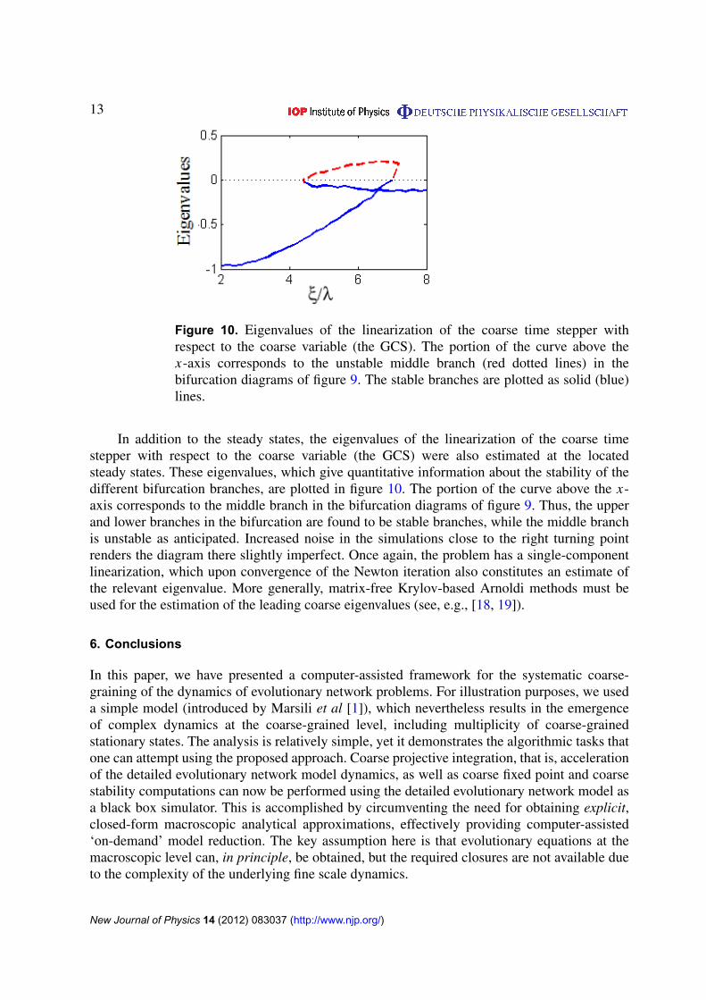
Figure 10. Eigenvalues of the linearization of the coarse time stepper withrespect to the coarse variable (the GCS). The portion of the curve above thex-axis corresponds to the unstable middle branch (red dotted lines) in thebifurcation diagrams of figure 9. The stable branches are plotted as solid (blue)lines.

In addition to the steady states, the eigenvalues of the linearization of the coarse timestepper with respect to the coarse variable (the GCS) were also estimated at the locatedsteady states. These eigenvalues, which give quantitative information about the stability of thedifferent bifurcation branches, are plotted in figure 10. The portion of the curve above the x-axis corresponds to the middle branch in the bifurcation diagrams of figure 9. Thus, the upperand lower branches in the bifurcation are found to be stable branches, while the middle branchis unstable as anticipated. Increased noise in the simulations close to the right turning pointrenders the diagram there slightly imperfect. Once again, the problem has a single-componentlinearization, which upon convergence of the Newton iteration also constitutes an estimate ofthe relevant eigenvalue. More generally, matrix-free Krylov-based Arnoldi methods must beused for the estimation of the leading coarse eigenvalues (see, e.g., [18, 19]).

6. Conclusions

In this paper, we have presented a computer-assisted framework for the systematic coarse-graining of the dynamics of evolutionary network problems. For illustration purposes, we useda simple model (introduced by Marsili et al [1]), which nevertheless results in the emergenceof complex dynamics at the coarse-grained level, including multiplicity of coarse-grainedstationary states. The analysis is relatively simple, yet it demonstrates the algorithmic tasks thatone can attempt using the proposed approach. Coarse projective integration, that is, accelerationof the detailed evolutionary network model dynamics, as well as coarse fixed point and coarsestability computations can now be performed using the detailed evolutionary network model asa black box simulator. This is accomplished by circumventing the need for obtaining explicit,closed-form macroscopic analytical approximations, effectively providing computer-assisted‘on-demand’ model reduction. The key assumption here is that evolutionary equations at themacroscopic level can, in principle, be obtained, but the required closures are not available dueto the complexity of the underlying fine scale dynamics.

New Journal of Physics 14 (2012) 083037 (http://www.njp.org/)

14

The illustrative model also serves to highlight some important issues that arise in this newcontext of adapting our coarse-graining framework to problems involving complex networkdynamics. The selection of good coarse variables is always an important and often a challengingstep. For this illustrative model, we established through numerical experimentation that theGCS is a good coarse variable to capture the slow dynamics, as other network statisticshave predominantly fast dynamics and get quickly slaved to the slow dynamics. We alsocreated a procedure for initializing networks (our ‘lifting’) consistent with slow dynamics.By computationally implementing our model reduction, we recovered the entire bifurcationdiagram with this single coarse variable, which suggests that this ‘effective one-dimensionality’holds over the entire parameter range we have studied. We should add that, within the equation-free framework, there are a number of additional tasks that can in principle be performed,such as the implementation of algorithms that converge on, and continue, higher codimensionbifurcation loci, or also algorithms that design stabilizing controllers for unstable coarsestationary states (see, e.g., [20]).

For many problems of interest, selection of the coarse-grained statistics is often done inan ad hoc manner or is based on intuition. Here we have demonstrated the use of simpledynamics arguments and computations to suggest ‘good’ coarse-grained observables, thatare subsequently used in equation-free computation. For more complex problems, where theappropriate observables for the coarse-grained description of the system’s behavior may beunknown, coupling the equation-free approach with nonlinear data mining approaches suchas diffusion maps [21, 22] appears to be a promising research direction. This would requirethe definition of a useful metric quantifying the distance between neighboring graphs (see,e.g., [23, 24]).

The computations in this paper were relatively simple, since the coarse descriptionconsisted of a single scalar variable. For problems where the coarse variables are many (suchas the for problems where a discretized coarse PDE must be solved), it is important to notethat one does not need to explicitly estimate each term in large Jacobian matrices. Matrix-freemethods (such as the Newton–Krylov GMRES) [17, 25] can be and have been used for theequation-free, time-stepper-based solution of large-scale coarse bifurcation problems [19]. Inour discussions of coarse projective integration, we demonstrated a tangible acceleration of thetemporal simulation of network evolution.

The computational saving from equation-free methods is obviously very problemdependent; for some problems simple direct simulation may be the easiest way to arrive at, say,a stable stationary state, rather than employing the equation-free machinery with its associatedcomputational overhead. There exist, however, tasks such as the location of unstable stationarystates, or the continuation of codimension one and higher bifurcations that would simply beimpossible through direct simulation, yet become accessible through our framework. As asimple rule of thumb, problems in which there exists a large separation of time scales betweenthe (slow) evolution of the coarse network evolution and the (fast) node-level dynamics probablypresent the greatest potential for computational saving. It is, of course, important to also notethat, if one is capable of analytically deriving accurate coarse-grained approximations, thecomputational saving would be so dramatic as to obviate the simulations with the detailedmodel—equation-free computations are precisely intended for situations in which coarse-grained equations are assumed to exist, but it is not possible to derive them in closed form.

Finally, the crux of the success of the approach lies almost invariably in the construction ofan efficient lifting algorithm—a step conceptually easy to describe, but often problem dependent

New Journal of Physics 14 (2012) 083037 (http://www.njp.org/)

15

and very challenging in itself. In the case of coarse-graining network dynamics, the problem ofconstructing networks with prescribed combinations of statistics is a notoriously difficult one,itself the subject of intensive research [26–34]. Given the interdependence of various networkstatistical properties, it is also important to be able to efficiently test the graphicality of a given‘prescription’—is a network with the prescribed set of statistics even feasible? We have madethis graphicality assumption every time we lifted in our paper because of the simplicity of oursingle coarse variable; however, this is a nontrivial problem when the coarse variables are severaland are also interdependent. In this context, we would also like to mention the systematic,integer linear programming-based approach of [35]. Clearly, algorithms capable of generatinggraphs with prescribed properties can be naturally integrated into the lifting step of the equation-free framework.

Acknowledgments

This work was partially supported by DTRA (HDTRA1-07-1-0005), the US AFOSR and theUS DOE (DE-SC0002097).

Appendix. A simple singularly perturbed system of ordinary differential equations

Let us consider a simple example of a singularly perturbed system of ordinary differentialequations for illustrative purposes:

dx

dt= 2 − x − y, (A.1)

dy

dt= 50(

√x − y). (A.2)

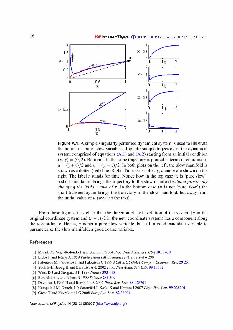
The top left panel of figure A.1 shows a solution trajectory of this set of equations startingfrom the initial condition (x, y) = (0, 2) as a solid (blue) line. The slow manifold of this set ofequations, represented by the curve y =

√x is plotted as a dotted (red) line. The trajectories of

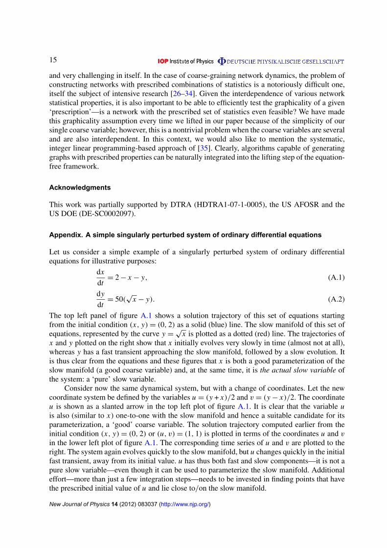
x and y plotted on the right show that x initially evolves very slowly in time (almost not at all),whereas y has a fast transient approaching the slow manifold, followed by a slow evolution. Itis thus clear from the equations and these figures that x is both a good parameterization of theslow manifold (a good coarse variable) and, at the same time, it is the actual slow variable ofthe system: a ‘pure’ slow variable.

Consider now the same dynamical system, but with a change of coordinates. Let the newcoordinate system be defined by the variables u = (y + x)/2 and v = (y − x)/2. The coordinateu is shown as a slanted arrow in the top left plot of figure A.1. It is clear that the variable uis also (similar to x) one-to-one with the slow manifold and hence a suitable candidate for itsparameterization, a ‘good’ coarse variable. The solution trajectory computed earlier from theinitial condition (x, y) = (0, 2) or (u, v) = (1, 1) is plotted in terms of the coordinates u and v

in the lower left plot of figure A.1. The corresponding time series of u and v are plotted to theright. The system again evolves quickly to the slow manifold, but u changes quickly in the initialfast transient, away from its initial value. u has thus both fast and slow components—it is not apure slow variable—even though it can be used to parameterize the slow manifold. Additionaleffort—more than just a few integration steps—needs to be invested in finding points that havethe prescribed initial value of u and lie close to/on the slow manifold.

New Journal of Physics 14 (2012) 083037 (http://www.njp.org/)

16

Figure A.1. A simple singularly perturbed dynamical system is used to illustratethe notion of ‘pure’ slow variables. Top left: sample trajectory of the dynamicalsystem comprised of equations (A.1) and (A.2) starting from an initial condition(x, y) = (0, 2). Bottom left: the same trajectory is plotted in terms of coordinatesu = (y + x)/2 and v = (y − x)/2. In both plots on the left, the slow manifold isshown as a dotted (red) line. Right: Time series of x , y, u and v are shown on theright. The label t stands for time. Notice how in the top case (x is ‘pure slow’)a short simulation brings the trajectory to the slow manifold without practicallychanging the initial value of x . In the bottom case (u is not ‘pure slow’) theshort transient again brings the trajectory to the slow manifold, but away fromthe initial value of u (see also the text).

From these figures, it is clear that the direction of fast evolution of the system (y in theoriginal coordinate system and (u + v)/2 in the new coordinate system) has a component alongthe u coordinate. Hence, u is not a pure slow variable, but still a good candidate variable toparameterize the slow manifold: a good coarse variable.

References

[1] Marsili M, Vega-Redondo F and Slanina F 2004 Proc. Natl Acad. Sci. USA 101 1439[2] Erdos P and Renyi A 1959 Publicationes Mathematicae (Debrecen) 6 290[3] Faloutsos M, Faloutsos P and Faloutsos C 1999 ACM SIGCOMM Comput. Commun. Rev. 29 251[4] Yook S-H, Jeong H and Barabasi A-L 2002 Proc. Natl Acad. Sci. USA 99 13382[5] Watts D J and Strogatz S H 1998 Nature 393 440[6] Barabasi A L and Albert R 1999 Science 286 509[7] Davidsen J, Ebel H and Bornholdt S 2002 Phys. Rev. Lett. 88 128701[8] Kumpula J M, Onnela J-P, Saramaki J, Kaski K and Kertesz J 2007 Phys. Rev. Lett. 99 228701[9] Gross T and Kevrekidis I G 2008 Europhys. Lett. 82 38004

New Journal of Physics 14 (2012) 083037 (http://www.njp.org/)

17

[10] Zschaler G, Traulsen A and Gross T 2010 New J. Phys. 12 093015[11] Huepe C, Zschaler G, Do A-L and Gross T 2011 New J. Phys. 13 073022[12] Kevrekidis I G, Gear C W, Hyman J M, Kevrekidis P G, Runborg O and Theodoropoulos C 2003 Commun.

Math. Sci. 1 715[13] Kevrekidis I G, Gear C W and Hummer G 2004 AIChE J. 50 1346[14] Lorenz E N 1986 J. Atmos. Sci. 43 1547[15] Gear C W and Kevrekidis I G 2005 J. Sci. Comput. 25 17[16] Zagaris A, Vadekerckhove C, Gear C W, Kaper T J and Kevrekidis I G 2012 Discrete Continuous Dyn. Syst.

32 2759[17] Kelley C T 1995 Iterative Methods for Linear and Nonlinear Equations (Frontiers in Applied Mathematics

16) (Philadelphia, PA: SIAM)[18] Anderson E et al 1999 LAPACK Users’ Guide (Philadelphia, PA: SIAM)[19] Siettos C I, Pantelides C C and Kevrekidis I G 2003 Ind. Eng. Chem. Res. 42 6795[20] Siettos C I, Armaou A, Makeev A G and Kevrekidis I G 2003 AIChE J. 49 1922[21] Nadler B, Lafon S, Coifman R R and Kevrekidis I G 2006 Appl. Comput. Harmon. A 21 113[22] Lafon S and Lee A B 2006 IEEE Trans. Pattern Anal. 28 1393[23] Borgs C, Chayes J, Lovasz L, Sos V and Vesztergombi K 2006 Topics in Discrete Mathematics: Algorithms

and Combinatorics (Berlin: Springer)[24] Vishwanathan S V N, Borgwardt K M, Risi Kondor I and Schraudolph N N 2008 arXiv:0807.0093[25] Saad Y and Schultz M H 1986 SIAM J. Sci. Stat. Comput. 7 856[26] Havel V 1955 Casopis Pest. Mat. 80 477[27] Dorogovtsev S N and Mendes J F F 2001 Phys. Rev. E 63 056125[28] Chung F and Lu L 2002 Ann. Comb. 6 125[29] Holme P and Kim B J 2002 Phys. Rev. E 65 026107[30] Klemm K and Eguıluz V M 2002 Phys. Rev. E 65 057102[31] Maslov S and Sneppen K 2002 Science 296 910[32] Volz E 2004 Phys. Rev. E 70 056115[33] Serrano M A and Boguna M 2005 Phys. Rev. E 72 036133[34] Leary C C, Schwehm M, Eichner M and Duerr H P 2007 Physica A 382 731[35] Gounaris C, Rajendran K, Kevrekidis I and Floudas C 2011 Optim. Lett. 5 435

New Journal of Physics 14 (2012) 083037 (http://www.njp.org/)