Coarse graining and control theory

model reduction

David E. Reynolds 1

ABSTRACT: We explain a method, inspired by control the-ory model reduction and interpolation theory, that rigorouslyestablishes the types of coarse graining that are appropriatefor systems with quadratic, generalized Hamiltonians. For suchsystems, general conditions are given that establish when lo-cal coarse grainings should be valid. Interestingly, our analysisprovides a reduction method that is valid regardless of whetheror not the system is isotropic. We provide the linear harmonicchain as a prototypical example. Additionally, these reductiontechniques are based on the dynamic response of the system,and hence are also applicable to nonequilibrium systems.

KEY WORDS: coarse graining; control theory; model reduc-tion; Hankel operator; operator theory

1Department of Physics, University of California,Santa Barbara, CA 93106

1

1 Introduction

Despite many of the great successes of statistical mechanics, it still lacksadequate methods for systematically treating heterogeneous and nonequi-librium systems. This is especially disconcerting considering that muchof the world about us is both heterogeneous and far from equilibrium. Inaddition, the treatment of open systems and systems with nontrivial bound-ary conditions have yet to be systematically incorporated into statisticalmechanics 2. It is not the purpose of this paper to address all of these defi-ciencies. Rather, we introduce techniques from control theory engineeringand interpolation theory to shed new light on such problems.

It is a standard practice in physics to simplify complicated systems. Inparticular limits, such as high-temperature or low-density, these idealiza-tions may become exact. We will discuss two of the main methods used inphysics to construct reduced-order models.

The projection-operator formalism (POF) of Mori and Zwanzig [6, 7, 5,12] is a method from nonequilibrium statistical mechanics. It allows contactbetween the constitutive conservative microscopic equations and the moremacroscopic phenomenological Langevin equations. The key mathematicalingredient in this approach, given an arbitrary observable, is to projectalong particular “directions” in state space in order to obtain an alternativeevolution equation involving contributions from a forcing term and froma memory kernel. Here the projections involved are simply integrationsover the appropriate phase space variables. A textbook application of thePOF is a particle in a heat bath [5, 8, 13, 2]. In this example, there isa clear split between important (system) variables and the less important(environment) variables. Thus, taking the system variables as the particle’sposition and momentum justifies projecting out the bath variables.

The renormalization group (RG) from field theory and equilibrium sta-tistical mechanics [33, 34], in its original form, involves identifying howthe physics of a system changes with scale. Equivalently, the renormal-ization group identifies how the parameters of a system’s Hamiltonian orLagrangian vary as the system is coarse grained. In the RG, systems are,almost invariably, locally coarse grained (i.e. locally-averaged). In thecontext of equilibrium statistical mechanics, the coarse graining is realizedwith the appropriate partial trace of a Boltzmann weight. Formally, thepartial trace is equivalent to the projections used in the POF.

An important observation is that both the POF and RG are completelygeneral techniques. Although typical system reductions are either based ona priori system-environment splits or obvious symmetries dictating localcoarse graining, there is enormous ambiguity in choosing which states to

2Of course the latter concern is somewhat atypical considering that boundary termsare usually deemed unimportant in the thermodynamic limit.

2

trace out 3. Intuition is enough of a guide for determining how to coarsegrain homogeneous systems with local interactions. However, without somedirection for dealing with heterogeneous systems, possibly with nonlocal in-teractions, the POF and RG are too general; they are useless. For instance,locally averaging about the interface in a layered system loses importantinformation about the system. Additionally, locally averaging such systemsis actually more likely to complicate the model. Complications arise sincethe averaged theory would pick up extra couplings to enforce the constraintof well-defined boundaries and induce couplings between the bulk of thedifferent layers. In short, for general systems, local coarse graining is likelyto discard important details. Consequently, as the effective influence ofthese discarded details is reincorporated into the coarsened description ofthe system, the new effective theory becomes increasingly complicated.

The above considerations support the view advocated in the work byBricmont and Kupiainen [37, 36, 35]. They contend that systems shouldnot be blindly coarse grained scale by scale, but rather, large fluctuationsshould remain fixed while those degrees of freedom corresponding to smallfluctuations are integrated away. A direct consequence of this perspectiveis that nonlocal coarse graining is on the same footing as its local counter-part. Intuitively, internal states that cause the largest fluctuations are themost relevant. The problem with such a program is that there exists nogeneral framework that allows for an unambiguous measure of the relativeimportance of a system’s internal degrees of freedom.

It is our claim that methods from control theory and modern interpo-lation theory provide a complete, general framework for determining howto appropriately coarse grain linear and linearly-dominated nonlinear sys-tems. Consequently, this opens up many new possible avenues to addressthe full nonlinear problem [27, 28, 29]. The primary idea of this approach isto coarse grain a system based on its dynamic response. For linear systems,it is possible to develop a completely unambiguous measure of how the in-ternal states of a system contribute to the response. In other words, it ispossible to assign a relative importance to the internal degrees of freedom.Determining this measure then dictates how the system should be coarsegrained. An especially nice feature of the control theory analysis is thatit decomposes the response into two separate, physically intuitive, parts:the controllability and observability of the internal states. Furthermore,these techniques are not limited to the idealized setting in which all of theinternal degrees of freedom of the system can be perfectly measured. Infact, these methods were tailored to deal with physical systems in an ex-

3Taking the partial trace of the probability density (Boltzmann weight) producesthe probability density for the corresponding random variable. Thus, the only realconstraint one should put on the partial trace is that it corresponds to a measurablerandom variable.

3

perimental setting! They are applicable even if the actuators and sensorsinterfaced with the system are imperfect. These methods are not only ofgreat theoretical use; they are of practical use as well.

In work by Hartle and Brun [10], it is speculated that local coarsegraining produces more deterministic effective equations of motion thannonlocal coarse graining. The problem with this claim is that it was madebased on investigating the homogeneous linear harmonic chain on ZN (i.e.on a ring) and considering a set of measure zero of all possible ways tocoarse grain the system. The main result of our paper rigorously establishesfor what (linear) systems the above claim is true and how it breaks downfor general linear systems. A primary instance when it breaks down isfor heterogeneous systems. We also establish how to appropriately coarsegrain systems when local coarse graining breaks down.

This paper serves two functions; (1) to introduce and integrate basicconcepts from control theory into standard physics problems, and (2) todevelop and apply a new algorithm for coarse graining that complementsexisting physical reduction techniques. In Section 2 we provide backgroundmaterial on the open loop control of linear systems. The definitions of con-trollability and observability are made precise. The controllability andobservability operators and gramians are then introduced. From these ob-jects, we establish a simultaneous measure of controllability and observ-ability. This measure specifies the relative importance of different internaldegrees of freedom. It also dictates how to model reduce or, equivalently,to coarse grain. Appendix A contains important details that generalizethe control theory model reduction techniques in Section 2 to conservativeand unstable systems. The lower bound in Appendix A is a new result.Lastly, in Section 3, we apply model reduction techniques to oscillator sys-tems to determine the “natural” reductions they admit. We see that undersome circumstances, depending on the spectral content of the system, localcoarse graining is valid. We also show how to coarse grain a system evenif it is not homogeneous and isotropic. Local coarse graining cannot beexpected to be appropriate for general quadratic Hamiltonians. In fact,our analysis shows the precise manner in which it is not. For illustrativepurposes, we examine the linear harmonic chain in detail.

2 A control theory tutorial

This section describes how control theory methods, in particular Hankelnorm analysis, may be used to determine the relative importance of theinternal degrees of freedom for arbitrary linear systems. A state’s impor-tance is directly related to its contribution to the system’s response. In thissection, we introduce the requisite control theory terminology and notation

4

that will be used throughout.In the opening subsection, we introduce the linear systems under inves-

tigation, their corresponding input-output behavior (response), and somerequisite material on the realization theory of input-output operators. Inthe next subsection, we provide definitions and measures of controllabil-ity and observability. The Hankel operator, its interpretation in terms ofcontrollability and observability, and its relation to balanced realizationscomprise the final subsection. The latter topics are especially important incontrol theory model reduction and, consequently, also for coarse graining.Although we made no attempt for this tutorial to be an exhaustive review,we include enough detail for the paper to be self-contained. All theoremsin this section are stated without proof. The interested reader is encour-aged to consult the following references [20, 24, 15, 16, 25]. Those who arealready familiar with the above concepts may comfortably skip ahead toSection 3.

2.1 Linear Systems and Realizations

This paper concerns linear time invariant (LTI) systems (i.e. linear systemswith time translation invariance) of the form:

x = Ax + Buy = Cx + Du

,

t ≥ t0,x(t) ∈ R

n,u(t) ∈ R

m,y(t) ∈ R

p,

(1)

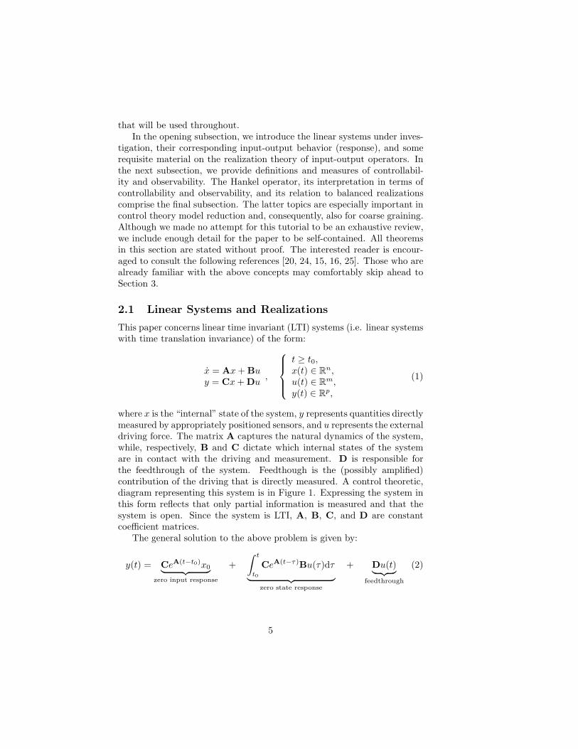
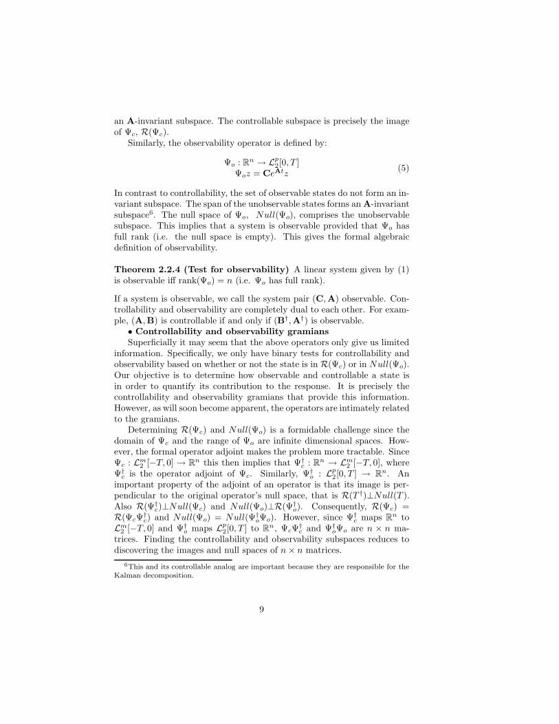
where x is the “internal” state of the system, y represents quantities directlymeasured by appropriately positioned sensors, and u represents the externaldriving force. The matrix A captures the natural dynamics of the system,while, respectively, B and C dictate which internal states of the systemare in contact with the driving and measurement. D is responsible forthe feedthrough of the system. Feedthough is the (possibly amplified)contribution of the driving that is directly measured. A control theoretic,diagram representing this system is in Figure 1. Expressing the system inthis form reflects that only partial information is measured and that thesystem is open. Since the system is LTI, A, B, C, and D are constantcoefficient matrices.

The general solution to the above problem is given by:

y(t) = CeA(t−t0)x0︸ ︷︷ ︸zero input response

+

∫ t

t0

CeA(t−τ)Bu(τ)dτ

︸ ︷︷ ︸zero state response

+ Du(t)︸ ︷︷ ︸feedthrough

(2)

5

If we consider only the zero state response (trivial initial conditions), then

y = Gu

=∫K(t, τ)u(τ)dτ =

∫ t

t0CeA(t−τ)Bu(τ)dτ.

(3)

The integral kernel has many names. In the time domain it is referred toas the impulse response or the Green’s function. Alternatively, for stable,LTI systems, the Fourier transform of the integral kernel is also knownas the transfer matrix, Green’s function in the frequency domain, or thepropagator. Since feedthrough is not crucial in our analysis, D = 0 fromthis point forward.

Figure 1: A block diagram representation of the linear system from 1 and 2.

Directed lines flowing into boxes represents vectors being multiplied by operators

(or matrices). For instance, initially u flows into B, hence the output of the first

box is Bu. The circles in the diagram are adders. Vectors that flow into adders

are summed.

In control theory, a system is specified by an experiment. This is re-flected by the dependence of G on B,C, and D. A system is defined by itsresponse (i.e. by G). From an experiment, the only available data is fromthe inputs and outputs. Hence, the matrices (A,B,C,D) are unknown.Constructing all of such matrices corresponding to a given response is theobjective of realization theory. The system matrices (A,B,C,D) forma state space realization of the system. For a given system, there doesnot exist a unique realization. However, given a realization, there existsa unique system. The choice of experiment fixes the system’s inputs andoutputs. The remaining ambiguity is due to the internal states of thesystem. For instance, an arbitrary invertible, linear change of variables,x = Rz, demonstrates this. (R−1AR,R−1B,CR,D) is also a realiza-tion of G. Since G is invariant under the above similarity transformations,realizations belong to equivalence classes. The remaining indeterminate-ness arises since there is not a bound on the number of internal degreesof freedom. In fact, there may be arbitrarily many internal states thatdo not contribute to the system’s response. State space realizations thathave the minimal internal state dimension are called minimal realizations

6

4. Although G is typically an infinite rank operator (i.e. the image of Gis infinite dimensional), the internal state dimension of its minimal realiza-tions gives it an order. When the minimal realization is stable, the orderof G is also known as its McMillan degree.

Minimal realizations represent the part of the system that is observ-able and controllable. To clarify this, we will introduce the definitions ofcontrollability and observability. We then define the controllability andoberservability operators along with their respective gramians. These con-cepts are imperative to assigning a measure of how much an individualinternal state contributes to the system’s response.

2.2 Controllability and Observability

• ControllabilityControllability concerns the effects of driving on the system. In particu-

lar, a system is controllable if it is possible to drive a system from any initial

configuration to any final configuration. An internal state of a system is

considered uncontrollable if it cannot be driven to every other state.

The issue of whether or not a system (or state) is controllable is ayes-or-no question. However, we may still intuitively assign a degree ofcontrollability to a state. An example of this is to consider the response of aconservative system when it is driven at one of its characteristic frequencies(at resonance). This is mathematically realized by a divergence (or a peak,in general) in the Fourier transform of the response. This is the simplestexample of a system’s mode being very controllable, insofar that we canelicit a large response from small amplitude driving5. It is easy to drivestates in the direction of this mode. Generally input-output resonancesdo not always correspond to internal resonances. Should there be a setor subspace of state or phase space that can not be reached via driving,then such “directions” are uncontrollable. A system is controllable if everydirection in state or phase space is controllable. The following provides amore formal and precise definition of controllability.

Definition 2.2.1 A system is controllable if it is possible to drive anyinitial state x0 to any final state xf in any nonzero time interval.

• ObservabilityObservability describes how easily the internal state of the system can

be reconstructed from measurements of the output. Intimately connected

4Minimal realizations of a given state dimension all belong to the same equivalenceclass.

5Driving with small amplitude is also termed driving or forcing with small gain.

7

to this is the precise determination of the internal initial conditions. Ini-

tial conditions that cannot be reconstructed are the system’s unobservable

states.

The mechanical model of a particle in a heat bath provides a physicalexample of observable versus unobservable states. As alluded to earlier,such as system admits a natural system-environment split. In this case thesystem is the single oscillator, while the environment is the bath. The oscil-lator is the primary object under investigation and hence, an experimentalapparatus is devised to measure its displacement and/or velocity. Since thebath is composed of innumerable constituent particles (or oscillators), theindividual trajectories of the bath particles are unknown. While the singleoscillator is strongly observable, the bath is only weakly observable. It ispossible to reconstruct the initial conditions for the single oscillator but notfor the entire bath. A more precise and formal definition of observabilityis:

Definition 2.2.2 A system is observable if it is possible to fully determineany initial state x0 by measuring y over any nonzero time interval.

• Controllability and observability operatorsIt is clear that the input-output operator, G, from equation (3) takes in

inputs from u from some space and outputs y in another. For concreteness,from now on we will consider the domain of G to be Lm

2 [−T, T ] (i.e. mcopies of L2) and the range to be Lp

2[−T, T ]. More generally, u may alsobe a vector in Lm

1 , Lm∞, or a Langevin contribution to the dynamics. The

construction of the controllability and observability operators, Ψc and Ψo

respectively, is largely motivated by the fact that the Hankel operator, tobe introduced later, can be factored into their product. Thus, the responsemay be decomposed into observability and controllability.

The controllability operator is defined by:

Ψc : Lm2 [−T, 0] → R

n

Ψcu =∫ 0

−Te−AτBu(τ)dτ =

∫ T

0eAτBu(−τ)dτ

(4)

Formally Ψc is not defined on the full domain of G. It can be extended tothe full space, however, by defining Lm

2 [0, T ] to be in its null space. Thecontrollability operator allows for an algebraic definition of controllability.

Theorem 2.2.3 A linear system, as in equation (1), specified by (A,B,C,D)is controllable if and only if the image of Ψc is all of R

n.

If a system in equation (1) is controllable, we call the system pair (A,B)controllable. Additionally, the space of states that are controllable forms

8

an A-invariant subspace. The controllable subspace is precisely the imageof Ψc, R(Ψc).

Similarly, the observability operator is defined by:

Ψo : Rn → Lp

2[0, T ]Ψoz = CeAtz

(5)

In contrast to controllability, the set of observable states do not form an in-variant subspace. The span of the unobservable states forms an A-invariantsubspace6. The null space of Ψo, Null(Ψo), comprises the unobservablesubspace. This implies that a system is observable provided that Ψo hasfull rank (i.e. the null space is empty). This gives the formal algebraicdefinition of observability.

Theorem 2.2.4 (Test for observability) A linear system given by (1)is observable iff rank(Ψo) = n (i.e. Ψo has full rank).

If a system is observable, we call the system pair (C,A) observable. Con-trollability and observability are completely dual to each other. For exam-ple, (A,B) is controllable if and only if (B†,A†) is observable.

• Controllability and observability gramiansSuperficially it may seem that the above operators only give us limited

information. Specifically, we only have binary tests for controllability andobservability based on whether or not the state is in R(Ψc) or in Null(Ψo).Our objective is to determine how observable and controllable a state isin order to quantify its contribution to the response. It is precisely thecontrollability and observability gramians that provide this information.However, as will soon become apparent, the operators are intimately relatedto the gramians.

Determining R(Ψc) and Null(Ψo) is a formidable challenge since thedomain of Ψc and the range of Ψo are infinite dimensional spaces. How-ever, the formal operator adjoint makes the problem more tractable. SinceΨc : Lm

2 [−T, 0] → Rn this then implies that Ψ†

c : Rn → Lm

2 [−T, 0], whereΨ†

c is the operator adjoint of Ψc. Similarly, Ψ†o : Lp

2[0, T ] → Rn. An

important property of the adjoint of an operator is that its image is per-pendicular to the original operator’s null space, that is R(T †)⊥Null(T ).Also R(Ψ†

c)⊥Null(Ψc) and Null(Ψo)⊥R(Ψ†o). Consequently, R(Ψc) =

R(ΨcΨ†c) and Null(Ψo) = Null(Ψ†

oΨo). However, since Ψ†c maps R

n toLm

2 [−T, 0] and Ψ†o maps Lp

2[0, T ] to Rn, ΨcΨ

†c and Ψ†

oΨo are n × n ma-trices. Finding the controllability and observability subspaces reduces todiscovering the images and null spaces of n × n matrices.

6This and its controllable analog are important because they are responsible for theKalman decomposition.

9

From the definition of the adjoint, the expression for Ψ†c is

Ψ†c : R

n → Lm2 [−T, 0],

Ψ†cz = B†e−A†tz For all z ∈ R

n, t ∈ [−T, 0].(6)

The following relation holds for Ψ†o:

Ψ†o : Lp

2[0, T ] → Rn,

Ψ†of =

∫ T

0 eA†τC†f(τ)dτ.(7)

From above, we are left with objects that are of fundamental importancefor establishing quantitative measures of controllability and observability,the gramians. The controllability gramian, Wc, is defined by:

Wc(T ) = ΨcΨ†c

=∫ T

0 eAtBB†eA†tdt.(8)

The observability gramian, Wo, is defined by:

Wo(T ) = Ψ†oΨo

=∫ T

0eA†tC†CeAtdt.

(9)

From their definitions, the gramians are both self-adjoint and positive semi-definite. Additionally, the controllable subspace of the system is the imageof Wc(T ). Thus, a linear system is controllable if and only if Wc(T ) isnonsingular (invertible). Similarly, the unobservability subspace is the nullspace of Wo(T ). A linear system is then observable if and only if Wo(T )is nonsingular (i.e. the null space is empty). Consequently, controllabilityand observability are determined by calculating two matrices, Wc(T ) andWo(T ). Equations (8) and (9) are computationally not very useful. It istypically easier to determine the gramians from the equations that theysatisfy.

dWc

dT= AWc + WcA

† + BB†; Wc(0) = 0 (10)

dWo

dT= A†Wo + WoA + C†C; Wo(0) = 0 (11)

For stable systems, in the limit as T → ∞, the gramians satisfy algebraicLyapunov equations 7.

7The Lyapunov equations are AWc+WcA†+BB

† = 0 and A†Wo+WoA+C

†C =

0.

10

x

x

1(a) (b)

n

x1

xn

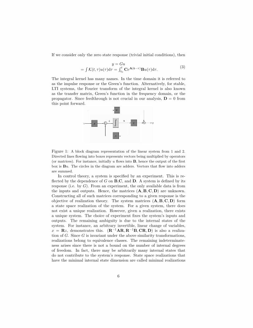
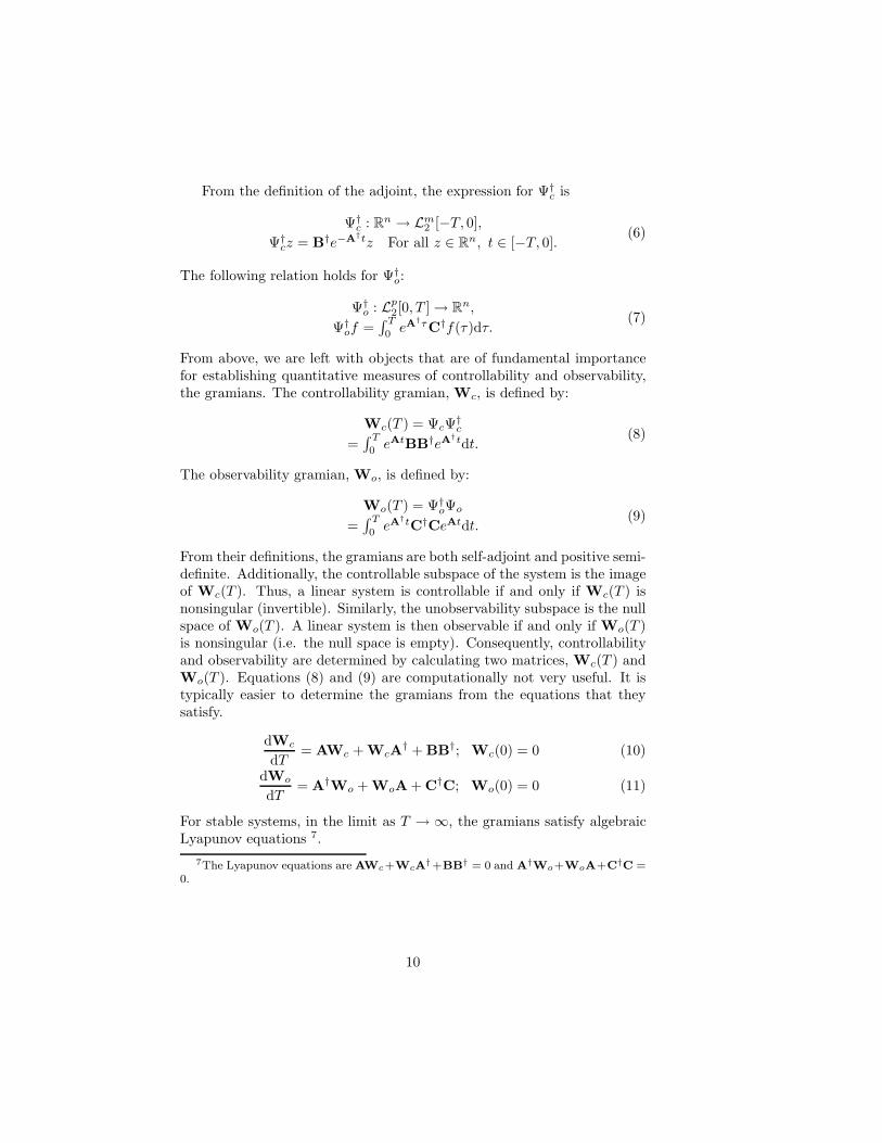
Figure 2: (a) depicts a controllability ellipsoid, while (b) depicts an observability

ellipsoid. The semimajor axis of the ellipsoid in (a) indicates the most controllable

direction in state space, and for the ellipsoid in (b) it indicates the most observable

direction.

The directions in state or phase space corresponding to trivial eigen-values of Wc are uncontrollable. Therefore, the eigenvectors of Wc cor-responding to small eigenvalues are only weakly controllable. It is alongthose directions that the controllability gramian is almost singular. Phys-ically, it requires much higher gains to reach these states than the morecontrollable states. More precisely, consider the quadratic energy func-

tional F (u) =∫ 0

−T ‖u(t)‖2Rmdt = ‖u‖2

Lm2 [−T,0] that measures the energy due

to driving. The u that expends the least energy to reach a state x ∈ Rn

from the origin 8 is given by umin = Ψ†cW

−1c x. The energy due to such

driving is‖umin‖2

Lm2 [−T,0] =

⟨umin, umin

⟩Lm

2

=⟨Ψ†

cW−1c x, Ψ†

cW−1c x

⟩Lm

2

=⟨x,W−1

c ΨcΨ†cW

−1c x

⟩Rn =

⟨x,W−1

c x⟩

Rn

= ‖W−1/2c x‖2

Rn .

(12)

If we drive the system in state or phase space with minimal force ‖umin‖2 ≤1, the corresponding region in state or phase space is a solid ellipsoid in R

n.This set, depicted in Figure 2(a), corresponds to x ∈ R

n : x†W−1c x ≤ 1.

This ellipsoid is also specified by x ∈ Rn : x = W

1/2c z, ‖z‖Rn ≤ 1. While

‖W−1/2c x‖2 measures energy expenditure,

‖W−1/2c x‖2

‖x‖2 = x†Wcxx†x

measures a

state’s controllability. This confirms the intuition that states correspondingto small eigenvalues of Wc are the least controllable.

Physically, the oberservability operator produces a response given aninitial condition. What does this reveal about the inverse problem of re-

8This is provided that the system is controllable and the dynamics of the system arerestricted to satisfy (1) with D = 0.

11

constructing the initial conditions from measurements of the system’s re-sponse? Mathematically this problem is posed as determining

minx∈Rn

‖y − Ψox‖2Lp

2 [0,T ].

When y is in the image of Ψo, it is possible to precisely specify the initialconditions, x. Otherwise, the initial condition minimizing ‖y−Ψox‖2

Lp2 [0,T ],

given an arbitrary y ∈ Lp2[0, T ], is xopt = W−1

o Ψ†oy. In order to ob-

tain a quantitative measure of observability, we need only consider theoutputs, y = Ψox. Immediately we recognize that ‖y‖2

Lp2 [0,T ]/‖x‖2

Rn =

‖W1/2o x‖2

Rn

∣∣‖x‖≤1

measures a state’s observability. For instance, initial

conditions, x, corresponding to small eigenvalues of Wo elicit smaller re-sponses than other states and, consequently, are less observable. If noiseis present, responses resulting from such initial conditions would not be

observed at all. The set x ∈ Rn : x = W

1/2c z, ‖z‖Rn ≤ 1 corresponds

to the observability ellipsoid depicted in Figure 2(b). The directions alongwhich the the ellipsoid is long are the most observable.

The utility in considering controllability and observability separately isthat they have precise and experimentally relevant interpretations. A prob-lem with this approach is that it initially obstructs the path to ascribingmeasures of response to physical states. For instance, it is possible to modelreduce based on either controllability or observability 9. Unfortunately,the measures of controllability and observability are not unique. This istransparent after considering how Wo and Wc transform under similarity

transformations to the system. Wo transforms as WoR−→ Wo = R†WoR,

while Wc transforms as WcR−→ Wc = R−1Wc(R

†)−1. Thus, the grami-ans are not invariant under an arbitrary linear coordinate transformation.

However, WcWo transforms as WcWoR−→ WcWo = R−1WcWoR un-

der a similarity transformation of the system. The eigenvalues of WcWo

are invariants of the system, are intimately related to the Hankel operatorof the system, and thus will prove invaluable for producing reduced-ordermodels.

2.3 The Hankel Operator, Balanced Realizations, andModel Reduction

The theory of model reduction is closely related to that of system realiza-tions. In model reduction, the goal is to find realizations (i.e. the matrices(A,B,C,D)) with minimal state dimension that approximately capture

9It has been shown in [4] that reductions based on the proper orthogonal decompo-sition (POD) is essentially equivalent to model reducing based on controllability.

12

the system’s input-output characteristics. Often being “near” the origi-nal system is enough to dramatically reduce the number of internal statesneeded to model the system. Here distance or “nearness” is defined by thestandard induced-operator norm. For example, given an operator S thatacts on L2, the induced norm takes the form ‖S‖L2,i = sup‖v‖L2≤1 ‖Sv‖L2 ,

where v is a vector in L2. Also, supposing that S approximates S, we willbe considering two measures of the error, the absolute error ‖S−S‖L2,i and

the relative error ‖S − S‖L2,i/‖S‖L2,i. The relative error is more appro-priate for unbounded operators, since most approximations are asymptoticestimates. The relative error is also the noise-to-signal ratio.

It is useful to note that there is an explicit expression for the inducedL2 norm for bounded (stable), LTI, causal operators. Such operators are inthe space H∞. The primary difficulty with this formula is that it is difficultto use both numerically and analytically. To motivate the formula, recallthat an arbitrary m×n matrix M can be decomposed as M = UΣV† (i.e.the singular value decomposition) where U and V are respectively m × mand n × n unitary matrices and Σ is only nontrivial along the diagonal.The diagonal values Σii = σi(M) ≥ 0 are called the singular values of

M. If m > n then the singular values are the eigenvalues of√

M†M,otherwise they are the eigenvalues of

√MM†. Here ‖M‖Cm,i = σmax(M)

where σmax(M) = maxj σj(M) (i.e. the largest singular value). For a

bounded, LTI, causal operator S such that S(u) =∫ t

−∞KS(t − τ)u(τ)dτ ,

‖S‖L2,i = supω∈R σmax(KS(ω)) where KS(ω) is the Fourier transform ofKS(t).

Coarse graining and model reduction are intimately related. Whileboth are reduction methods, coarse graining emphasizes the spatial natureof reductions. Model reduction, as it will be presented here, emphasizesinput-output resonances and approximating the response. Our approachto coarse graining is to identify the best way to model reduce, based onthe response, and then ascertain the spatial structure of the reduction.The latter topic is elaborated upon for linear oscillator systems in the nextsection. Unfortunately, the former issue is a mathematically unresolvedproblem. The control/interpolation theoretic statement of this problem forstable systems (in the induced L2-norm) is called the H∞ model reductionproblem.

Definition 2.3.1 (H∞ Model Reduction Problem) Given a bounded,LTI, causal operator G of McMillan degree n, such that G : L2 → L2, findinfdeg(G)≤k ‖G − G‖L2,i for G a bounded, LTI, causal operator and k < n.

Fortunately, enough is known about a related problem, the Hankel normmodel reduction problem, to provide error bounds to the above H∞ prob-lem. By using results from Hankel operator analysis and Hankel norm

13

model reduction, we will be able to deduce physically-important resultsabout coarse graining.

• The Hankel operatorThe input-output picture corresponds to an experimental situation, al-

beit a complicated one. The full input-output operator, G, from y = Gurepresents continuously driving and measuring a system. This operator isdifficult to study because it does not separate observation from driving. Aswill become apparent, the Hankel operator is the part of the input-outputoperator where the operations of measurement and forcing are separated.

To facilitate analysis, it is convenient to decompose L2[−T, T ] intoL2[−T, 0] ⊕ L2[0, T ], in other words, a causal (analytic) decomposition.LTI causal systems can be visualized in the following way:

[y−y+

]=

[G11 G12

G21 G22

] [u−

u+

]=

[ TG 0

ΓG TG

] [u−

u+

],

y+ ∈ Lp2[0, T ],

y− ∈ Lp2[−T, 0],

u+ ∈ Lm2 [0, T ],

u− ∈ Lm2 [−T, 0].

(13)

Causality implies that G12 = 0. The additional constraint that the systemis LTI implies that K(t, τ) is purely a function of t − τ . TG and TG areToeplitz operators, while ΓG is a Hankel operator. It is not vital norrequired for the reader to be familiar with Hankel or Toeplitz operators.The interested reader is encouraged to consult [17, 18, 19, 21, 22, 23, 15, 16]to learn more about these operators. If we denote the projection operatoronto L2[0, T ] by P+, then P 2

+ = P+ and ΓG = P+G∣∣L2[−T,0]

. Since such

projection operators can never increase the norm, it follows that ‖ΓG‖ ≤‖G‖. Similarly, ‖TG‖ = ‖TG‖ ≤ ‖G‖, where the first equality arises since

TG and TG differ only by time reversal. A somewhat surprising fact is that‖TG‖ = ‖G‖ [17]. Model reduction based on TG is equivalent to the full H∞

problem for stable systems. Unfortunately, the experiments represented byTG involve simultaneously driving and observing.

The Hankel operator, ΓG, accepts inputs driving the internal state tosome x0 at time t = 0. Subsequently, the system is measured as it evolvesin time. The separation of driving and measurement allows for ΓG to befactored in the particularly convenient way:

ΓG(u) = P+G∣∣L2[−T,0]

u = P+

∫ 0

−TCeA(t−τ)Bu(τ)dτ

= P+CeAt∫ 0

−T e−AτBu(τ)dτ = ΨoΨcu.(14)

The Hankel operator may be factored as a product of the observability

14

operator and controllability operator: ΓG = ΨoΨc. It follows that

‖ΓG‖2L2,i = ‖Γ†

GΓG‖L2,i

= ‖Ψ†cΨ

†oΨoΨc‖L2,i = ‖Ψ†

oΨoΨcΨ†c‖Rn,i

= ‖WoWc‖Rn,i = ‖√

WoWc‖2Rn,i

= σ2max(

√WoWc).

(15)

In fact, if the system is controllable and observable, the entire nonzerospectrum of Γ†

GΓG can be obtained.

nonzero squared singular values of ΓG = nonzero eigenvalues of Γ†GΓG

= nonzero eigenvalues of Ψ†cΨ

†oΨoΨc = eigenvalues of Ψ†

oΨoΨcΨ†c

= eigenvalues of WoWc = eigenvalues of WcWo

(16)The singular values of ΓG are called the Hankel singular values (HSV).The nonzero HSV are the eigenvalues of

√WcWo, the set of invariants

mentioned at the end of the previous subsection.The Hankel norm model reduction problem is useful for finding bounds

for the full H∞ model reduction problem. In particular, it establishes theHSV as a measure of response.

Definition 2.3.2 (Hankel Norm Model Reduction Problem) Givena rank n Hankel operator ΓG corresponding to a stable, causal, LTI systemG, such that ΓG : Lm

2 [−T, 0] → Lp2[0, T ], find infrank(Γ)≤k ‖ΓG − Γ‖L2,i for

Γ a Hankel operator and k < n.

In order to motivate the solution to the above problem, we first need tointroduce the following theorem.

Theorem 2.3.3 Given a rank n matrix M ∈ Rp×r (n ≤ min(p, r)) with

nonzero singular values ordered such that σ1(M) ≥ σ2(M) ≥ . . . ≥ σn(M),for an arbitrary rank m matrix S ∈ R

p×r such that m ≤ k < n,

σmax(M − S) ≥ σk+1(M) (17)

Combining (13) and (15) and Theorem 2.3.3 leads to the next theorem.This is fundamental to this paper, for it solves the Hankel model reductionproblem.

Theorem 2.3.4 Given a rank n Hankel operator ΓG with nonzero singularvalues ordered such that σ1(ΓG) ≥ σ2(ΓG) ≥ . . . ≥ σn(ΓG), for an arbitraryrank k Hankel operator Γ such that k < n,

‖ΓG − Γ‖L2,i ≥ σk+1(ΓG) (18)

15

A limitation of this theorem is that, for finite dimensional systems, theredoes not always exist a Hankel operator that makes the inequality an equal-ity.

When equation (18) is combined with ΓG = P+G|L2[−T,0], we obtain alower bound for G.

For order(G) = n (i.e. McMillan Degree n),

For all G of order k ≤ r, ‖G − G‖L2,i ≥ σr+1(ΓG)(19)

An interpretation of this lower bound is that the best possible rth-orderapproximation to the input-output behavior of the system is at least a“distance” σr+1(ΓG) away from the exact response. It implies that anyreduced order model that projects out states corresponding to large singularvalues is necessarily a worse approximation than a model that projects outsmall singular values. Thus, states corresponding to large singular valuescontribute the most to the system’s response.

• Balanced realizationsIt has been shown that the nonzero HSV correspond to the eigenvalues

of√

WcWo. This suggests that the Hankel operator is related to thesystem’s controllability and observability. This connection is importantfor many reasons. Firstly, interpreting the Hankel operator in terms ofobservability and controllability aids intuition. Secondly, the gramians’eigenvalues are not invariant under coordinate transformations, so we stilllack unambiguous measures of controllability and observability. Lastly,as we can see in Figure 2, controllability and observability may not becorrelated. For generic realizations, observability and controllability arenot on the same footing and consequently this leads to further ambiguity.Should model reduction be based on observability or controllability?

The resolution to these problems relies on determining the most suit-able coordinates. This is equivalent to ascertaining the proper way to coarsegrain the system. Our freedom in the choice of coordinates allows us to finda coordinate transformation, T, such that, in the new coordinates, the con-trollability and observability gramians are equal and diagonal. The readermay note that this procedure is essentially the same as is used in filteringtheory. This aligns the observability and controllability ellipsoids, therebyputting controllability and observability on the same footing. Furthermore,

in these balanced coordinates, Wc = Wo = Σ where Σ is diagonal and hasthe same eigenvalues as

√WcWo (ordered from largest to smallest). The

eigenvalues of the balanced gramians are the nonzero HSV, invariants of thesystem. The resulting system realization is known as a balanced realization.

T can be constructed using the following algorithm [20]. By definition,there exists a coordinate transformation S such that S−1WcWoS = Σ2.Now supposing that S = W

−1/2o R for some R, R−1W

1/2o WcW

1/2o R = Σ2.

16

Hence, W1/2o WcW

1/2o is Hermitian and similar to Σ2. Provided Σ does

not have degenerate eigenvalues, there exists a unique unitary matrix U

such that U†W1/2o WcW

1/2o U = Σ2. This means that

(Σ−1/2U†W1/2o )Wc(Σ

−1/2U†W1/2o )† = Σ.

Thus, remembering that Wc transforms as WcT−→ Wc= T−1Wc(T

†)−1,

if we let T−1 = Σ−1/2U†W1/2o , we have found the desired coordinate

transformation. It follows that:

T†WoT =(Σ1/2U†W

−1/2o

)Wo

(W

−1/2o UΣ1/2

)

= Σ1/2U†UΣ1/2 = Σ.(20)

In general, if a system is not controllable and observable, such a T (bal-ancing transformation) does not exist. It is possible to find a balancingtransformation such that:

Wc =

Σ 0 0 00 Σ1 0 00 0 0 00 0 0 0

and Wo =

Σ 0 0 00 0 0 00 0 Σ2 00 0 0 0

, (21)

where Σ,Σ1, and Σ2 are all diagonal. Σ is the matrix of HSV and thecorresponding subsystem is controllable and observable. The subsystem as-sociated with Σ1 is controllable and unobservable, while the one associatedwith Σ2 is uncontrollable and observable.

• Balanced truncationNow we possess the tools to generate reduced-order models. The re-

duction technique in what follows is called balanced truncation. We assumethat the system is stable, controllable and observable, and has been trans-formed into a balanced realization. Additionally, since the system is stable,we consider the problem over an infinite time horizon (i.e. T → ∞).

Given a system satisfying the above assumptions, decompose the matrixof ordered HSV Σ (ordered from largest to smallest) such that the first reigenvalues form the matrix ΣL. The remainder form the matrix of smallersingular values ΣS . Decompose ΣL and ΣS such that they have no commoneigenvalues. The realization for the full system takes the form:

A =

[AL A12

A21 AS

], B =

[BL

BS

],

C =[

CL CS

].

(22)

By projecting out the states corresponding to ΣS , the remaining three ma-trices, (AL, BL, CL), form an r-dimensional realization that approximates

17

the original system. Denote the input-output operator for the reduced sys-tem by Gr . This realization, by construction, is stable and balanced. ItsHSV are the eigenvalues of ΣL. In additional, the approximation error isgiven by:

‖G − Gr‖L2,i ≤ 2

k∑

j=1

σdistij

, (23)

where σdistij

: 1 ≤ j ≤ k is the distinct HSV in ΣS .These techniques are extended to unstable systems in Appendix A. This

makes it possible to use these techniques on linear, conservative systems.A particularly relevant result is:

Theorem 2.3.5 (Lower Bound) Given a LTI, causal system G with ndimensional minimal realization (A,B,C). If there exists an “a” such that−aI+A is a stable system matrix then for any order r (or less) approximantGr

‖G − Gr‖L2[0,T ],i ≥(1 − e−2aT ‖eA†T eAT ‖Cn,i

)σr+1(a)

It is the subject of the next section to apply these methods to generaloscillator systems, whereupon, when combined with the spatial content ofthe reductions, specifies how to coarse grain.

3 Reduction of Oscillator Systems

The standard form for the equations of motion generated by a quadraticHamiltonian with 2N phase space degrees of freedom is given by

[qp

]=

[0 Ω

−Ω 0

] [qp

], (24)

where Ω is a N×N positive definite matrix. These systems are typically as-sociated with coupled harmonic oscillators. Furthermore, these systems areconsidered trivial because when expressed in normal modes, the resultingoscillators are decoupled. Decoupled oscillators are considered noninteract-ing. This view is correct for isolated systems, however, for open systems itis not.

The coordinates that capture the original experimental configuration isof exceptional interest. This is because the important coordinate system formodel reduction is the one in which the gramians are balanced. Now whilein balanced coordinates the gramians are diagonalized, the matrices A orΩ need not be. This illustrates that a generic open system, even a linearone, typically has interacting internal states. The statistical mechanics ofquadratic Hamiltonians is invalid unless the system is driven. This follows

18

since when expressed in normal modes, the system is noninteracting and,hence, not ergodic or mixing [13, 14]. The usual heuristic argument forjustifying the practice is that phonon (oscillator) systems do not truly havea linear dispersion; the systems themselves are nonlinear. The nonlinearityis responsible for the mixing of states. This is precisely the issue thatspawned the Fermi-Pasta-Ulam (FPU) problem 10. Once the nonlinearityfrom the heuristic argument is associated to a disturbance of the formBu(t), then the analysis in this paper agrees with the heuristic argument.

The advantages of using balanced coordinates rather than modal coordi-nates reflect the sensitivity of the system to the choice of experiment. Thissensitivity to experiment suggests that it is more appropriate for oscillatorsystems 11 to investigate open systems.

z =

[z1

z2

]= Az + Bu =

[0 I

−Ω2 0

] [z1

z2

]+ Bu

y = Cz(25)

In this coordinate system, z1 represents the spring displacements while z2

represents the corresponding velocities.There remains the question of which experiments should be considered.

Conceptually, B varies the gains of the driving. B determines how accessi-ble particular states are to driving. Alternatively, allowing for Dirac deltadriving and setting z0 = 0, the driving may be used to prepare the sys-tem’s initial conditions. With this interpretation, B prescribes how initialconditions are weighted. Similarly, C indicates which and how easily inter-nal states are measured. We exclusively consider oscillator systems withuniform constituent sizes and masses. This choice, motivated by thermody-namics and the equipartition of energy, implies that positions and momentaare treated equally. This is equivalent to assuming that the position andmomentum of each particle can be driven with equal gain. Hence, B = bI,where b is a constant. Considering each position and momentum equallydifficult to measure corresponds to setting C = cI. Now let b = c = 1.Mathematically this choice is natural since the resulting input-output op-erator (in the Laplace domain) is the full system’s resolvent, (sI − A)−1.

Fixing B and C dictates the type of experiment. However, it does notfully determine the experiment. For the problem to be well-posed, we alsoneed to specify the duration of the experiment. This is important becausethe exact form of the experiment fully determines its input-output charac-teristics (i.e. the input-output operator). Different experiments give rise

10It is interesting to note that coupled, nonlinear, anharmonic oscillator systems arenot guaranteed to mix. This fact has been attributed to the existence soliton solutionsto the equations of motions.

11At least oscillator systems with uniform masses.

19

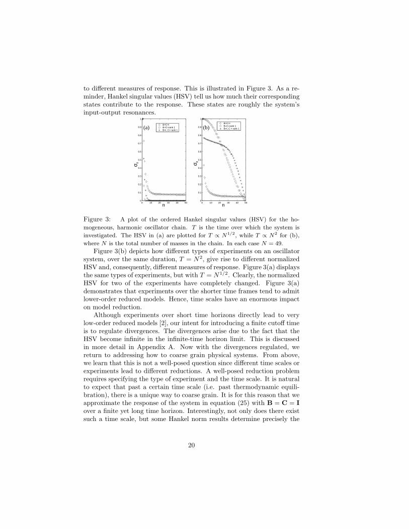
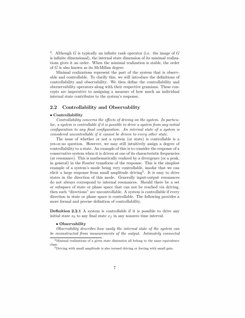
to different measures of response. This is illustrated in Figure 3. As a re-minder, Hankel singular values (HSV) tell us how much their correspondingstates contribute to the response. These states are roughly the system’sinput-output resonances.

0 10 20 30 40 500

0.1

0.2

0.3

0.4

0.5

0.6

0.7

0.8

0.9

1

0 10 20 30 40 500

0.1

0.2

0.3

0.4

0.5

0.6

0.7

0.8

0.9

1

B=C=IB=C=rank 1B=I, C = rank 1

B=C=IB=C=rank 1B=I, C= rank 1

n n

(b)(a)

nσ σ n

Figure 3: A plot of the ordered Hankel singular values (HSV) for the ho-

mogeneous, harmonic oscillator chain. T is the time over which the system is

investigated. The HSV in (a) are plotted for T ∝ N1/2, while T ∝ N2 for (b),

where N is the total number of masses in the chain. In each case N = 49.

Figure 3(b) depicts how different types of experiments on an oscillatorsystem, over the same duration, T = N2, give rise to different normalizedHSV and, consequently, different measures of response. Figure 3(a) displaysthe same types of experiments, but with T = N1/2. Clearly, the normalizedHSV for two of the experiments have completely changed. Figure 3(a)demonstrates that experiments over the shorter time frames tend to admitlower-order reduced models. Hence, time scales have an enormous impacton model reduction.

Although experiments over short time horizons directly lead to verylow-order reduced models [2], our intent for introducing a finite cutoff timeis to regulate divergences. The divergences arise due to the fact that theHSV become infinite in the infinite-time horizon limit. This is discussedin more detail in Appendix A. Now with the divergences regulated, wereturn to addressing how to coarse grain physical systems. From above,we learn that this is not a well-posed question since different time scales orexperiments lead to different reductions. A well-posed reduction problemrequires specifying the type of experiment and the time scale. It is naturalto expect that past a certain time scale (i.e. past thermodynamic equili-bration), there is a unique way to coarse grain. It is for this reason that weapproximate the response of the system in equation (25) with B = C = Iover a finite yet long time horizon. Interestingly, not only does there existsuch a time scale, but some Hankel norm results determine precisely the

20

coarse grainings. These topics comprise the following subsections, the firstin which we work without restriction on the form of Ω other than that it ispositive definite. In the second subsection we consider the case of the ho-mogeneous linear harmonic chain, and lastly we treat some heterogeneouslinear oscillator chains.

3.1 General Oscillator Systems

To determine the best possible coarse graining or at least near the optimalcoarse graining, we will proceed to use the Hankel operator machinery toobtain bounds for ‖G − Gr‖L2[0,T ],i. Recalling the control theory tutorial,this provides us with a criterion for model reduction. In particular, thelower bound,

‖G − G‖L2,i ≥ σr+1(ΓG),

where σr+1(ΓG) is the (r + 1)th HSV, confirms that the states with largeHSV contribute the most to the response. The upper bound,

‖G − G‖L2,i ≤ 2

k∑

j=1

σdistij

,

where σdistij

: 1 ≤ j ≤ k is the set of distinct HSV with ij > r, ensuresthat our approximations are controlled. The first step is to determine theHSV that provide these bounds. However, in doing so we also find thebalancing transformation. This makes it trivial to truncate the system andobtain reduced-order models.

Determining the HSV requires calculating the controllability and ob-servability gramians. Unfortunately, restricting attention to a finite cutofftime complicates the analysis. For instance, Wc and Wo satisfy differentialequations (see equations (10) and (11)) instead of Lyapunov equations. Amethod of simplifying the analysis involves investigating the system ma-trix −aI + A over an infinite time horizon instead of A over a finite timehorizon. This procedure is known as exponential discounting. Intuitively“a” should be on the order of the inverse time cutoff for the approximationto be any good. Fortunately the above intuition can be made much morerigorous, thereby keeping all approximations under control.

For the systems under consideration, the gramians are formally givenby

Wc =∫ T

0 eAteA†tdt ⇒ W(a)c =

∫ ∞

0 e−2ateAteA†tdt,

Wo =∫ T

0eA†teAtdt ⇒ W

(a)o =

∫ ∞

0e−2ateA†teAtdt.

(26)

A property of these gramians is that WcWo or W(a)c W

(a)o are always

similar to a matrix of the form

[M 00 M†

]. This means that there is

21

an exact duplicity in the HSV independent of “a”. In fact, under thetransformation R defined in Appendix B, A takes the form of the system

matrix in equation (24). In this basis, we find that Wc ≈ Wo where

Wc = 14a

[Ω + Ω−1 + O(a2) 0

0 Ω + Ω−1 + O(a2)

]

+ 14

[0 Ω−2 − I + O(a2)

Ω−2 − I + O(a2) 0

].

(27)

In this basis the gramians are almost balanced. Provided we transform the

system by a unitary transformation, Ud, to diagonalize Ω (i.e. ΩUd−→ ΛΩ)

and we take “a” sufficiently small (sufficiently long-time horizons), thegramians are balanced. The precise interpretation of “sufficiently small” isoutlined in Appendix C. We want to require that “a” is small enough sothat the off-diagonal terms do not change the ordering of the HSV. Here weassume, without loss of generality, that the eigenvalues of ΛΩ are orderedfrom smallest to largest. Under the previously mentioned conditions toO(a2) the balanced gramians (balanced up to permutation) take the form

Wc = Wo =1

4a

[ΛΩ + Λ−1

Ω + O(a2) O(a)O(a) ΛΩ + Λ−1

Ω + O(a2)

]. (28)

These balanced gramians are associated with the linear system[

˙z1

˙z2

]=

[0 ΛΩ

−ΛΩ 0

] [z1

z2

]+

[Λ

1/2Ω U†

d 0

0 Λ−1/2Ω U†

d

] [u1

u2

],

[y1

y2

]=

[UdΛ

−1/2Ω 0

0 UdΛ1/2Ω

] [z1

z2

].

(29)Given that λj(Ω) ≤ λk(Ω) for all j < k, let α be a permutation suchthat λα(j)(Ω) + λ−1

α(j)(Ω) ≤ λα(k)(Ω) + λ−1α(k)(Ω) for all k < j. Trivially,

via a unitary transformation, the gramians in equation (28) may be fullybalanced (the HSV are ordered). In this case, we find that

σk(a) =1

4a

(λdα(k)

2 e(Ω) + λ−1

dα(k)2 e

(Ω))

+ O(1). (30)

The degeneracy of the HSV suggests that any balanced truncation thatkeeps states corresponding to the first r = 2q HSV will remain conservative.In fact, we can see this by inspection of equation (29). With this in mind,we will consider only truncations that keep an even number of states. Theimmediate consequences of these results are that we obtain bounds on theapproximation error of the response.

‖G − G2q‖L2[0,T ],i ≥(1 − e−2aT

)σ2q+1(a)

=1

4a(1 − e−2aT )

(λα(q+1)(Ω) + λ−1

α(q+1)(Ω)),

(31)

22

and

‖G − G2q‖L2[0,T ],i ≤ 2eaTN−1∑

j=q

σ2j+1(a)

=1

2aeaT

N∑

j=q+1

λα(j)(Ω) + λ−1α(j)(Ω).

(32)

Additionally, by using linear-matrix-inequality (LMI) techniques [26], asubstantially tighter upper bound can be established. The improved boundis

‖G − G2q‖L2[0,T ],i ≤ 2eaT σ2k+1(a)= 1

2aeaT(λα(k+1)(Ω) + λ−1

α(k+1)(Ω)).

(33)

A remarkable aspect of these oscillator models is that, over a long timehorizon, the relation between the system’s spectrum and the gramians issimple. Despite this simple relationship, these results also establish thatthe set of best reductions (i.e. those that satisfy the lower bound) neednot be modal reductions! Modal reductions explicitly neglect (project out)the system’s fast dynamics. For instance, let us suppose that λj(Ω) ≥ 1for all j; disregarding degeneracy, the HSV are automatically ordered fromsmallest to largest. This implies that projecting out small HSV eliminatesstates corresponding to slow modes! This is contrary to what is typicallydone. Alternatively, suppose that λj(Ω) < 1 for all j. In this instance,disregarding degeneracy, the HSV are ordered from largest to smallest.This is precisely when modal reduction is appropriate. Lastly, when theeigenvalues of Ω are both greater than and less than one, the appropriatereductions involve a mixing of fast and slow modes.

In the basis that produces the realization in equation (29), the systemis balanced, and yet Ω is diagonalized. Although this means that suchsystems are noninteracting, not all internal states are treated equally. Infact, in the case of the linear harmonic chain, the weighting of the gainshas a physically meaningful interpretation that will be elaborated uponin Section 3.2. Also, there is an enormous degeneracy in the types ofexperiments producing equivalent reductions. The same reductions resultfrom using B = V and C = U where V and U are arbitrary unitarymatrices. This may not come as much of a surprise since requiring V andU to be unitary causes the internal states to be treated equally. We seethat there are an infinite number of inequivalent realizations that yield thesame reduction.

These results also reveal how to choose “a”. By varying “a” we mayrefine our bounds. Generally, we have an LTI, causal system that achievesor almost achieves the lower bound. Consequently, it is useful to choose“a” such that the lower bound is at its maximum. The maximum occurs

23

as a → 0.

‖G − G2q‖L2[0,T ],i ≥T

2

(λα(q+1)(Ω) + λ−1

α(q+1)(Ω))

(34)

For the lowest upper bound (from balanced truncation), dda

[2eaT σ2k+1(a)

]=

0 implies that a = T−1. Therefore, the minimum upper bound is

‖G − G2q‖L2[0,T ],i ≤eT

2

(λα(q+1)(Ω) + λ−1

α(q+1)(Ω)). (35)

As we approximate G over an infinite-time horizon (T → ∞), both thenorm of G and the absolute error diverge. This divergence is unavoidableand generally independent of the number of particles (oscillators) in thesystem. However, there is another possible interpretation if the numberof particles, N , is large. For our analytics to be valid, there must berestrictions on the size of “a”. Combining equations (71) and (73) fromAppendix C, we are able to relate the maximal “a” to the frequenciesof the system, λk(Ω). In most cases, as N gets large, λk(Ω) ∼ N−δ1 .For instance, in the case of the homogeneous linear harmonic chain, forsmall wave number, δ1 = 1. Consequently, “a” is forced to fall to zeroasymptotically like a ∼ N−δ2 for some δ2 > 0 as N → ∞. Reciprocally,if “a” tends to zero faster and, consequently, T tends to infinity, thereis no restriction on N . The divergence is due to the infinite time horizon.Suppose that “a” is parameterized by N and we consider the N → ∞ limit.In this case, the divergence is due to the infinite-particle limit. For oscillatorsystems, like photons and phonons, the divergence is attributable to theabsence of a mass gap (i.e. the eigenvalues of Ω become dense near zero).Thus, there is no inherent length (mass) scale for the system. This is one ofthe simplest divergences, a long wavelength divergence. Depending on thestructure of ΛΩ, however, there may also be a short-wavelength divergenceor even possibly a mixed-wavelength divergence. Had we investigated yet ashorter time scale, still taking T → ∞, the resulting reduced-order systemsare typically dissipative [3, 2]. Physically this is a manifestation of howfluctuations may induce time scales [13, 14].

While the divergence in ‖G‖L2,i and ‖G − Gr‖L2,i has been explained,its consequences have not. Since the error estimate diverges, except whenregulated (i.e. by considering finite T ), the absolute error is not a meaning-ful quantity. Any long-time approximate is asymptotic at best. This meansthat the (regulated) relative error, limT→∞ ‖G − Gr‖L2[0,T ],i/‖G‖L2[0,T ],i,is much more useful. Combining equations (31) and (32) yield rather con-

24

servative bounds:

limT→∞

‖G − G2q‖L2[0,T ],i

‖G‖L2[0,T ],i≥ lim

T→∞

T2

(λα(q+1)(Ω) + λ−1

α(q+1)(Ω))

eT2

∑Nj=1 λα(j)(Ω) + λ−1

α(j)(Ω)

=λα(q+1)(Ω) + λ−1

α(q+1)(Ω)

eTr(Ω + Ω−1

) ,

(36)

and

limT→∞

‖G − G2q‖L2[0,T ],i

‖G‖L2[0,T ],i≤ lim

T→∞

eT2

∑Nj=q+1 λα(j)(Ω) + λ−1

α(j)(Ω)

T2

(λα(1)(Ω) + λ−1

α(1)(Ω))

=e∑N

j=q+1 λα(j)(Ω) + λ−1α(j)(Ω)

(λα(1)(Ω) + λ−1

α(1)(Ω)) .

(37)

Comparatively tighter bounds are obtained by using equations (34) and(35). These bounds are

limT→∞

‖G − G2q‖L2[0,T ],i

‖G‖L2[0,T ],i≥

λα(q+1)(Ω) + λ−1α(q+1)(Ω)

e(λα(1)(Ω) + λ−1

α(1)(Ω)) , (38)

and

limT→∞

‖G − G2q‖L2[0,T ],i

‖G‖L2[0,T ],i≤

e(λα(q+1)(Ω) + λ−1

α(q+1)(Ω))

λα(1)(Ω) + λ−1α(1)(Ω)

. (39)

These general cases have allowed us, for instance, to determine condi-tions when modal reduction is appropriate. Without knowing more aboutΩ it is not possible to discern the spatial content of the reductions. Withoutthe spatial content we cannot specify the relationship between reductiontype and coarse graining. In the following section, we will apply the aboveresults to the linear harmonic chain, from which we determine the appro-priate coarse grainings. This example will clarify the relationship betweensystem reductions and coarse grainings.

3.2 The Linear Harmonic Chain

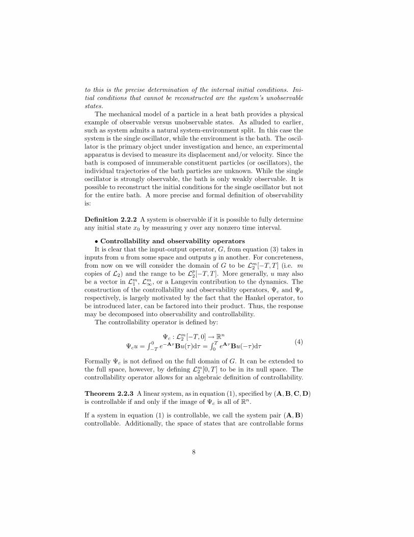
The models that we consider in this section are all variants of the one-dimensional linear harmonic chain depicted in Figure 4. The system con-sists of a chain of N equally spaced masses each with mass m connected viaN +1 springs. The chain is connected on each side to stationary walls. Wewill first treat coarse graining the linear harmonic chain with homogeneoussprings in great detail. Briefly, we also present how to coarse grain someheterogeneous chains. We will conclude by comparing the different modelsand their respective coarse grainings.

25

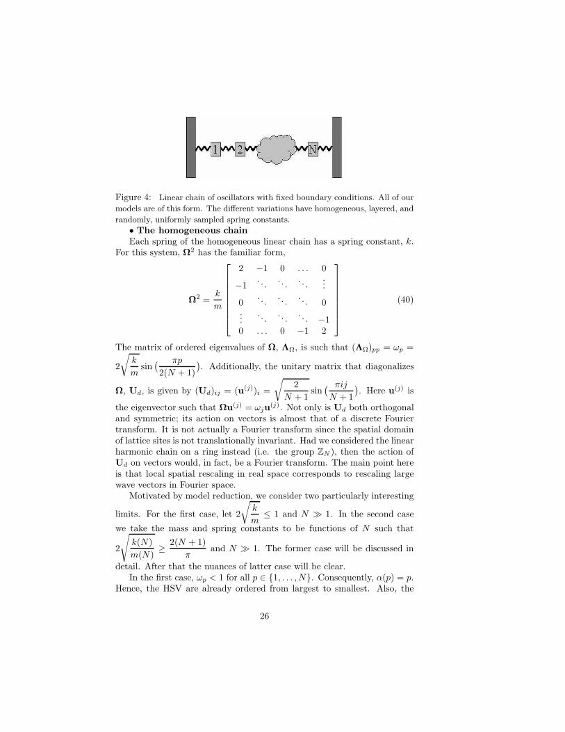
Figure 4: Linear chain of oscillators with fixed boundary conditions. All of our

models are of this form. The different variations have homogeneous, layered, and

randomly, uniformly sampled spring constants.

• The homogeneous chainEach spring of the homogeneous linear chain has a spring constant, k.

For this system, Ω2 has the familiar form,

Ω2 =k

m

2 −1 0 . . . 0

−1. . .

. . .. . .

...

0. . .

. . .. . . 0

.... . .

. . .. . . −1

0 . . . 0 −1 2

(40)

The matrix of ordered eigenvalues of Ω, ΛΩ, is such that (ΛΩ)pp = ωp =

2

√k

msin

( πp

2(N + 1)

). Additionally, the unitary matrix that diagonalizes

Ω, Ud, is given by (Ud)ij = (u(j))i =

√2

N + 1sin

( πij

N + 1

). Here u(j) is

the eigenvector such that Ωu(j) = ωju(j). Not only is Ud both orthogonal

and symmetric; its action on vectors is almost that of a discrete Fouriertransform. It is not actually a Fourier transform since the spatial domainof lattice sites is not translationally invariant. Had we considered the linearharmonic chain on a ring instead (i.e. the group ZN ), then the action ofUd on vectors would, in fact, be a Fourier transform. The main point hereis that local spatial rescaling in real space corresponds to rescaling largewave vectors in Fourier space.

Motivated by model reduction, we consider two particularly interesting

limits. For the first case, let 2

√k

m≤ 1 and N 1. In the second case

we take the mass and spring constants to be functions of N such that

2

√k(N)

m(N)≥ 2(N + 1)

πand N 1. The former case will be discussed in

detail. After that the nuances of latter case will be clear.In the first case, ωp < 1 for all p ∈ 1, . . . , N. Consequently, α(p) = p.

Hence, the HSV are already ordered from largest to smallest. Also, the

26

minimal time scale over which this analysis is valid is determined by thelimits on “a”. When “a” satisfies the inequality in equation (73), whichimplies “a” at least scales as N−2 (if not faster in N), the ordering of theHSV is not altered. This gives the absolute error bounds when combinedwith the expression for ωp and equations (34) and (35).

‖G − G2q‖L2[0,T ],i ≥ T2

(sin

( π(q+1)2(N+1)

)+

(sin

( π(q+1)2(N+1)

))−1)

= NTπ(q+1)

(1 + O

( (q+1N

)2 )) (41)

‖G − G2q‖L2[0,T ],i ≤ eT2

(sin

( π(q+1)2(N+1)

)+

(sin

( π(q+1)2(N+1)

))−1)

= eNTπ(q+1)

(1 + O

( (q+1N

)2 )) (42)

It is no surprise that the appropriate reductions project out the fastmodes since in this limit the dispersion is linear. In the limit of large N ,truncating fast modes is the same as projecting out large wave numbers.However, as mentioned earlier, large wave numbers correspond to shortdistances. So we see that projecting out fast modes from this system isequivalent to locally coarse graining. In fact, the lower bound suggestsa stronger result. Provided the lower bound is approximately achievable,though the reduced-order system may not be LTI, the best possible reduc-tions must involve locally coarse graining (modally reducing) the system.For example, projecting out a slow mode via balanced truncation is anexample of nonlocal coarse graining. The lower bound of the incurred ap-proximation error involves the HSV corresponding to that nonlocal state.Since the HSV corresponding to slow (nonlocal) modes are larger thanthose of fast modes, any nonlocal approximant of the system is necessarilyworse by equation (41).

0 10 20 30 40 500

0.1

0.2

0.3

0.4

0.5

0.6

0.7

0.8

0.9

1

0 10 20 30 40 500

0.1

0.2

0.3

0.4

0.5

0.6

0.7

0.8

0.9

1

n n

(a) (b)

ωnnσ

Figure 5: (a) A plot of the ordered Hankel singular values (HSV) for the homo-

geneous, harmonic oscillator chain. The spring constants are uniformly taken to

27

be k = 0.25. The HSV are plotted for T ∝ N2 where N = 49. The distribution

of HSV remains essentially unchanged for any larger choice of T . (b) A plot of

the frequencies for the same system.

The bounds in equations (41) and (42) also, at least for this model, pro-vide information regarding finite size effects. If we take the lattice spacingto be b and the system size of the approximate system to be L = qb, thebounds then imply that (for N 1)

limT→∞

‖G − G2q‖L2[0,T ],i

‖G‖L2[0,T ],i= O(L−1). (43)

This result is not new, though these techniques provide a new way to obtainit. Additionally, these techniques imply that for more general systemsor experiments, reductions may have quite a different dependence on thesystem size.

It is apparent from (29) that the balanced realization for the harmonic

chain weights driving of the momenta by Λ−1/2Ω Ud. Since (ΛΩ)pp = ωp

N1−→πp2N , this gives more weight to momenta corresponding to small frequencies.Therefore it requires smaller gains to activate the slower modes. If drivinggives nontrivial initial conditions (i.e. impulses), this is equivalent to slow-mode initial conditions being more easily excited than fast-mode initialconditions. While the balanced realization of the system implies that theinternal states of the system are noninteracting, it also implies that differingnormal modes are not treated equally. This again suggests that the mostnatural coarse grainings are local coarse grainings.

Consider the latter conditions mentioned earlier, 2

√k(N)

m(N)≥ 2(N + 1)

π

and N 1. Here ωp > 1 for all p ∈ 1, . . . , N and implies that α(p) =N +1− p. The upper and lower bounds for this case are respectively givenby

‖G − G2q‖L2[0,T ],i ≥ T2

(cos

( π(q+1)2(N+1)

)+

(cos

( π(q+1)2(N+1)

))−1)

= NTπ

(1 − π2(q+1)2

4N2 + O( (

q+1N

)4 )),

(44)

and

‖G − G2q‖L2[0,T ],i ≤ eT2

(cos

( π(q+1)2(N+1)

)+

(cos

( π(q+1)2(N+1)

))−1)

= eNTπ

(1 − π2(q+1)2

4N2 + O( (

q+1N

)4 )).

(45)

This system is rather pathological since any good approximant must haveq ∝ N , as seen in equation (44). It is impossible for the error to be

28

made small unless q is of the same order as N . That q must scale as Nimplies that this system does not admit the same nice reductions as theprevious example. Recall that for the previous example the relative errorvanishes as N → ∞ as long as q ∝ N δ for any δ such that 0 < δ < 1.Thus, decent reductions must retain far more states than the previousexample. Despite this pathology, the appropriate reductions project outthe slower modes. Since the same Ud may be used as before (i.e. essentiallya Fourier transform), the coarse graining keeps the small distance behavior(fast modes) and projects out the rest. For this system, high-frequencymodes are more easily amplified, which explains the importance of includingthose modes in the approximate response.

• The layered and random chainsWhen Ud is not a Fourier transform then these amenable dispersion re-

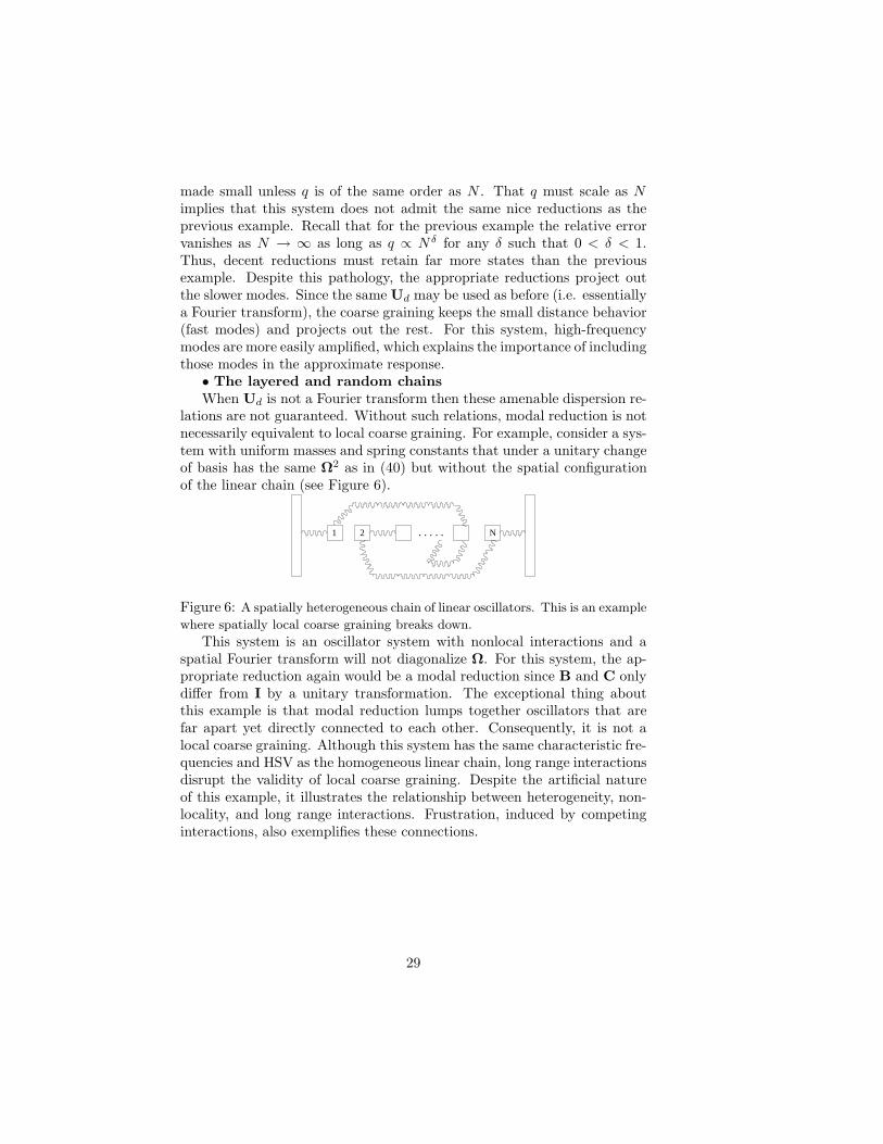
lations are not guaranteed. Without such relations, modal reduction is notnecessarily equivalent to local coarse graining. For example, consider a sys-tem with uniform masses and spring constants that under a unitary changeof basis has the same Ω2 as in (40) but without the spatial configurationof the linear chain (see Figure 6).

. . . . .1 N2

Figure 6: A spatially heterogeneous chain of linear oscillators. This is an example

where spatially local coarse graining breaks down.

This system is an oscillator system with nonlocal interactions and aspatial Fourier transform will not diagonalize Ω. For this system, the ap-propriate reduction again would be a modal reduction since B and C onlydiffer from I by a unitary transformation. The exceptional thing aboutthis example is that modal reduction lumps together oscillators that arefar apart yet directly connected to each other. Consequently, it is not alocal coarse graining. Although this system has the same characteristic fre-quencies and HSV as the homogeneous linear chain, long range interactionsdisrupt the validity of local coarse graining. Despite the artificial natureof this example, it illustrates the relationship between heterogeneity, non-locality, and long range interactions. Frustration, induced by competinginteractions, also exemplifies these connections.

29

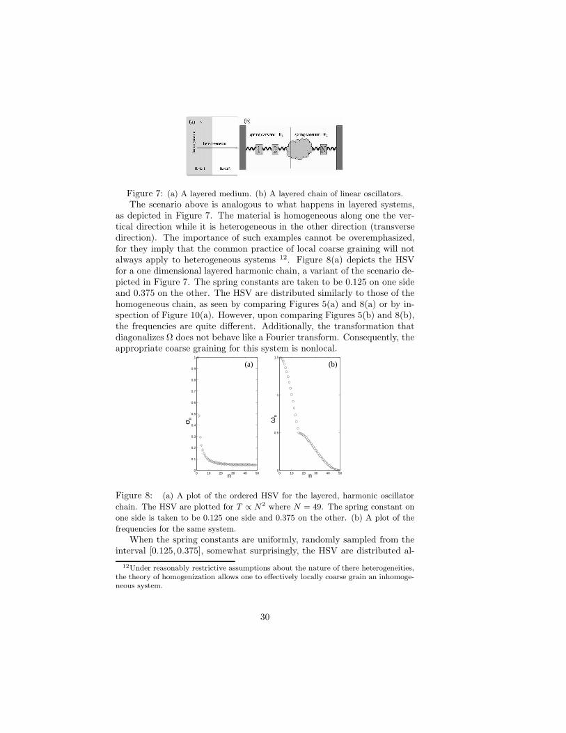
Figure 7: (a) A layered medium. (b) A layered chain of linear oscillators.

The scenario above is analogous to what happens in layered systems,as depicted in Figure 7. The material is homogeneous along one the ver-tical direction while it is heterogeneous in the other direction (transversedirection). The importance of such examples cannot be overemphasized,for they imply that the common practice of local coarse graining will notalways apply to heterogeneous systems 12. Figure 8(a) depicts the HSVfor a one dimensional layered harmonic chain, a variant of the scenario de-picted in Figure 7. The spring constants are taken to be 0.125 on one sideand 0.375 on the other. The HSV are distributed similarly to those of thehomogeneous chain, as seen by comparing Figures 5(a) and 8(a) or by in-spection of Figure 10(a). However, upon comparing Figures 5(b) and 8(b),the frequencies are quite different. Additionally, the transformation thatdiagonalizes Ω does not behave like a Fourier transform. Consequently, theappropriate coarse graining for this system is nonlocal.

0 10 20 30 40 500

0.1

0.2

0.3

0.4

0.5

0.6

0.7

0.8

0.9

1

0 10 20 30 40 500

0.5

1

1.5

n n

(a) (b)

nσ ωn

Figure 8: (a) A plot of the ordered HSV for the layered, harmonic oscillator

chain. The HSV are plotted for T ∝ N2 where N = 49. The spring constant on

one side is taken to be 0.125 one side and 0.375 on the other. (b) A plot of the

frequencies for the same system.

When the spring constants are uniformly, randomly sampled from theinterval [0.125, 0.375], somewhat surprisingly, the HSV are distributed al-

12Under reasonably restrictive assumptions about the nature of there heterogeneities,the theory of homogenization allows one to effectively locally coarse grain an inhomoge-neous system.

30

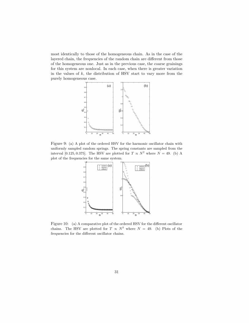
most identically to those of the homogeneous chain. As in the case of thelayered chain, the frequencies of the random chain are different from thoseof the homogeneous one. Just as in the previous case, the coarse grainingsfor this system are nonlocal. In each case, when there is greater variationin the values of k, the distribution of HSV start to vary more from thepurely homogeneous case.

0 10 20 30 40 500

0.1

0.2

0.3

0.4

0.5

0.6

0.7

0.8

0.9

1

0 10 20 30 40 500

0.2

0.4

0.6

0.8

1

1.2

1.4

n n

(a) (b)

ωnnσ

Figure 9: (a) A plot of the ordered HSV for the harmonic oscillator chain with

uniformly sampled random springs. The spring constants are sampled from the

interval [0.125, 0.375]. The HSV are plotted for T ∝ N2 where N = 49. (b) A

plot of the frequencies for the same system.

0 10 20 30 40 500

0.1

0.2

0.3

0.4

0.5

0.6

0.7

0.8

0.9

1

0 10 20 30 40 500

0.5

1

1.5

randomlayereduniform

randomlayereduniform

n n

(a) (b)

nσ

nω

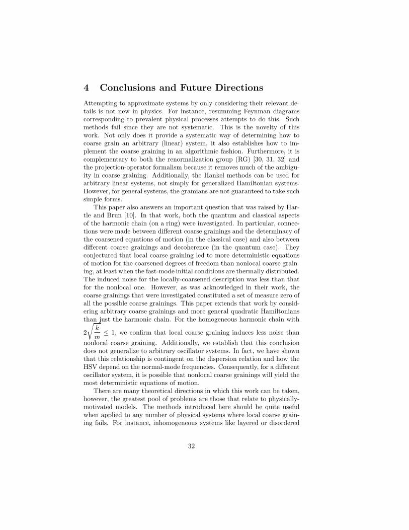
Figure 10: (a) A comparative plot of the ordered HSV for the different oscillator

chains. The HSV are plotted for T ∝ N2 where N = 49. (b) Plots of the

frequencies for the different oscillator chains.

31

4 Conclusions and Future Directions

Attempting to approximate systems by only considering their relevant de-tails is not new in physics. For instance, resumming Feynman diagramscorresponding to prevalent physical processes attempts to do this. Suchmethods fail since they are not systematic. This is the novelty of thiswork. Not only does it provide a systematic way of determining how tocoarse grain an arbitrary (linear) system, it also establishes how to im-plement the coarse graining in an algorithmic fashion. Furthermore, it iscomplementary to both the renormalization group (RG) [30, 31, 32] andthe projection-operator formalism because it removes much of the ambigu-ity in coarse graining. Additionally, the Hankel methods can be used forarbitrary linear systems, not simply for generalized Hamiltonian systems.However, for general systems, the gramians are not guaranteed to take suchsimple forms.

This paper also answers an important question that was raised by Har-tle and Brun [10]. In that work, both the quantum and classical aspectsof the harmonic chain (on a ring) were investigated. In particular, connec-tions were made between different coarse grainings and the determinacy ofthe coarsened equations of motion (in the classical case) and also betweendifferent coarse grainings and decoherence (in the quantum case). Theyconjectured that local coarse graining led to more deterministic equationsof motion for the coarsened degrees of freedom than nonlocal coarse grain-ing, at least when the fast-mode initial conditions are thermally distributed.The induced noise for the locally-coarsened description was less than thatfor the nonlocal one. However, as was acknowledged in their work, thecoarse grainings that were investigated constituted a set of measure zero ofall the possible coarse grainings. This paper extends that work by consid-ering arbitrary coarse grainings and more general quadratic Hamiltoniansthan just the harmonic chain. For the homogeneous harmonic chain with

2

√k

m≤ 1, we confirm that local coarse graining induces less noise than

nonlocal coarse graining. Additionally, we establish that this conclusiondoes not generalize to arbitrary oscillator systems. In fact, we have shownthat this relationship is contingent on the dispersion relation and how theHSV depend on the normal-mode frequencies. Consequently, for a differentoscillator system, it is possible that nonlocal coarse grainings will yield themost deterministic equations of motion.

There are many theoretical directions in which this work can be taken,however, the greatest pool of problems are those that relate to physically-motivated models. The methods introduced here should be quite usefulwhen applied to any number of physical systems where local coarse grain-ing fails. For instance, inhomogeneous systems like layered or disordered

32

systems are prime nontrivial candidates. Additionally, this work is ide-ally suited for nonequilibrium systems. In particular, since it identifies thedegrees of freedom that seem both most “excitable” and “observable”, itmay be appropriate for revealing the true nature of effective temperatures[11]. For granular systems, this would be a big step towards identifying theimportance of such mysterious quantities as the granular temperature andthe free volume. Accordingly, it is in these directions, among others, thatfuture work using these methods should be taken.

Acknowledgments

The author thanks Professors J. Hartle and I. Mezic for the conversationsthat culminated into this paper. Special thanks are also due to C. Maloneyfor his many questions and criticisms of this work. This work has alsobenefited from comments by Professor D. Cai. Lastly, the encouragementsand suggestions from K. Reynolds and Professor J. Carlson are greatlyappreciated and have been crucial to the completion of this work. This workwas supported by the David and Lucile Packard Foundation, NSF GrantNo. DMR-9813752, and EPRI/DoD through the Program on InteractiveComplex Networks.

A Infinite time horizon results for finite timehorizon problems

Approximating conservative linear systems over an infinite time horizoninevitably leads to divergences. This may be understood from the factthat the gramians become unbounded due to the infinite time horizon. Astandard way to regulate this divergence is by approximating the systemover a finite time horizon. Alternatively, the system can be exponentiallydiscounted and considered over an infinite time horizon.

In this appendix we express the upper and lower bounds for the approx-imation of the input-output operator over a finite time horizon in terms ofexponentially-discounted infinite-time-horizon Hankel singular values. Al-though this analysis is only applied to conservative systems, we find thebounds for arbitrary finite dimensional systems that admit LTI, causal real-izations. Given a system realization (A,B,C), we denote the input-outputoperator and its order r approximant respectively by G and Gr. Similarly,for the exponentially discounted system (i.e. with system matrix −aI+A),the input-output operator and its approximant are denoted by G(a) and

G(a)r , respectively. Additionally, the finite time horizon HSV are given by

33

σ1 ≥ σ2 ≥ . . . ≥ σn while the infinite time horizon singular values are givenby σ1(a) ≥ σ2(a) ≥ . . . ≥ σn(a).

Equation (19) as it is stated is equally valid for infinite or finite timehorizons. However, we intend to relate ‖G − Gr‖L2[0,T ],i to the singularvalues σi(a) : 1 ≤ i ≤ n. The following new theorem establishes therelation of interest.

Theorem A.0.1 (Lower Bound) Given a LTI, causal system G with ndimensional minimal realization (A,B,C). If there exists an “a” such that−aI+A is a stable system matrix then for any order r (or less) approximantGr

‖G − Gr‖L2[0,T ],i ≥(1 − e−2aT ‖eA†T eAT ‖Cn,i

)σr+1(a)

Proof :Since the Hankel operator is simply a projection of the original input

output operator we initially trivially find for an arbitrary Gr,

‖G − Gr‖L2[0,T ],i ≥ ‖ΓG − ΓGr‖L2[0,T ],i ≥ ‖ΓG −Kr‖L2[0,T ],i, (46)

where Kr is an arbitrary rank r operator that is not restricted to be ofHankel form. The last inequality arises because it is known that ‖ΓG −ΓGr

‖L2[0,T ],i ≥ σ(ΓG) and equality is not always possible since ΓGris of

Hankel form. However, equality is achievable for an arbitrary operator Kr.The primary nontrivial step in this proof requires the observation that

the each of the eigenvalues of the balanced gramian, W (a), associated toΓG(a) = Γ(a) are decreasing functions of a. This can be seen by noting thatfor any vector ζ ∈ R

n and for b < a,

⟨ζ,

(W (b) − W (a)

)ζ⟩≥ 0. (47)

This means that σk(a) ≤ σk(b) for a > b. From this observation it is thenfollows that

‖ΓG −Kr‖L2[0,T ],i ≥ ‖Γ(a) − Kr‖L2[0,T ],i. (48)

Then using that for any two bounded linear operators, A and B, in theinduced norm ‖AB‖ ≤ ‖A‖‖B‖ and that

‖eAT ‖Cn,i = ‖eA†T eAT ‖1/2Cn,i, (49)

we finally obtain

‖Γ(a) − Kr‖L2[0,T ],i ≥ ‖Γ(a) − Kr‖L2[0,∞],i − ‖Γ(a) − Kr‖L2[T,∞],i

≥(1 − e−2aT ‖eA†T eAT ‖Cn,i

)σr+1(a).

(50)

34

Hence we arrive at the desired result,

‖G − Gr‖L2[0,T ],i ≥(1 − e−2aT ‖eA†T eAT ‖Cn,i

)σr+1(a). (51)

In the case where A has no Jordan blocks the above result simplifies to

‖G − Gr‖L2[0,T ],i ≥(1 − e2T max Re λ(−aI+A)

)σr+1(a). (52)

This lower bound is completely consistent with (19) for stable systems.Although we only use the upper bound in determining the relative error,we include it in the following. Recall from equation (23) that the upperbound is only valid for stable systems (for infinite time). In fact, it is almostexclusively proven for stable systems in the literature. The following upperbounds, valid for finite time horizon, are taken from [1].

Theorem A.0.2 (Upper Bound) Given a LTI, causal system G with ndimensional minimal realization (A,B,C), if “a” is such that −aI + A isa stable system matrix and ‖G(a)‖L2,i < γ, then:

‖G‖L2[0,T ],i < γeaT

Proof : This results follows from the differential version of the bounded reallemma. For details refer to [1].

We already know from equation (23) how to obtain an upper bound

for the approximation error, ‖G(a) − G(a)r ‖L2,i. We combine this fact with

Theorem A.0.2 to obtain the following corollary.

Corollary A.0.3 (Upper Bound) Given a LTI, causal system G with ndimensional minimal realization (A,B,C), if “a” is such that −aI + A isa stable system matrix then there exists an order r input-output operator,Gr obtained by balanced truncation such that

‖G − Gr‖L2[0,T ],i < 2eaTk∑

j=1

σdistij

(a),

where σdistij

(a), 1 ≤ j ≤ k are the distinct infinite time horizon HSV from

the set σr+1(a), . . . , σn(a).

To be precise, an algorithm to obtain Gr is as follows. First find the real-

ization for G(a)r by truncating the balanced realization of (−aI+ A,B,C).

Denote the resulting realization by (Ar ,Br,Cr). A realization for Gr isthen just (aI + Ar,Br,Cr).

35

B Calculation of the Gramians

In this appendix we intend to calculate the balanced form of the gramiansfor oscillator systems (i.e. of systems of the form found in equation (25)).This entails calculating the damped (exponentially discounted) gramians:

W(a)c =

∫ ∞

0e−2ateAteA†tdt

W(a)o =

∫ ∞

0 e−2ateA†teAtdt(53)

However, first let us introduce the following notations and conventions.Recall that any matrix, S, may be expressed in terms of the canonicalmatrix units, eij . In other words,

S =∑

i,j

Sijeij

where each Sij is just a complex number. For instance, in the case of 2× 2matrices,

e12 =

[0 10 0

]

Additionally, for this section, Q =

[0 1−1 0

]. Lastly, we frequently use

the algebraic tensor product, ⊗ 13. For instance, suppose

A =

[A11 A12

A21 A22

]

then

A ⊗ B =

[A11B A12BA21B A22B

]

First note that if we define

R = e11 ⊗ Ω−1/2 + e22 ⊗ Ω1/2 (54)

then easily it follows that

A = e12 ⊗ I − e21 ⊗ Ω2 =

[0 I

−Ω2 0

]

R−→ R−1AR = Q ⊗ Ω =

[0 Ω

−Ω 0

] (55)

From this, one then finds that

W(a)c = R

∫ ∞

0e−2ateQ⊗ΩtR−1R−1e−Q⊗ΩtdtR

= R∫ ∞

0e−2ateQ⊗Ωt

[Ω 00 Ω−1

]e−Q⊗ΩtdtR

(56)

13Often referred to as the dyadic product.

36

However, using that eQ⊗Ωt = I ⊗ cosΩt + Q ⊗ sinΩ we finally arrive at

W(a)c = R

∫ ∞

0 e−2at×[Ω cos2 Ωt + Ω−1 sin2 Ωt 1

2Ω−1(Ω−1 − Ω) d

dt sin2 Ωt12Ω

−1(Ω−1 − Ω) ddt sin2 Ωt Ω−1 cos2 Ωt + Ω sin2 Ωt

]dt R

= 14aR

[Ω + Ω−1 0

0 Ω + Ω−1

]R + 1

4aR×[

−a2Ω−1(I − Ω2)(a2I + Ω2)−1 a(I − Ω2)(a2I + Ω2)−1

a(I − Ω2)(a2I + Ω2)−1 a2Ω−1(I − Ω2)(a2I + Ω2)−1

]R.

(57)Similarly for the observability gramian we obtain

W(a)o = 1

4aR−1

[Ω + Ω−1 0

0 Ω + Ω−1

]R−1 + 1

4aR−1×[

a2Ω−1(I − Ω2)(a2I + Ω2)−1 a(I − Ω2)(a2I + Ω2)−1

a(I− Ω2)(a2I + Ω2)−1 −a2Ω−1(I − Ω2)(a2I + Ω2)−1

]R−1.

(58)From equations (57) and 58 it follows after using Ud to diagonalize Ω

and taking the small “a” limit that the balanced gramian, without orderedeigenvalues, is given by

Wc = Wo =1

4a

[ΛΩ + Λ−1

Ω + O(a2) O(a)O(a) ΛΩ + Λ−1

Ω + O(a2)

].

C Restrictions on the time horizon/exponentialdiscounting

C.1 Relevant matrix perturbation

We start with a matrix Lε of the form,

Lε =

(M εNεN M

). (59)

The question we intend to address is, how do the ε terms perturb thespectrum of L0.

det(λI − Lε) = det

(λI − M −εN−εN λI − M

)

= det

(λI − M −εN

0 λI − M − ε2N(λI − M)−1N

)

= det(λI − M

)det

(λI − M − ε2N(λI − M)−1N

)

=(det(λI − M)

)2det

(I − ε2

((λI − M)−1N

)2)

(60)

37

However, recall that given an invertible matrix P,

P−1 =(det(P)

)−1adj(P), (61)

where adj is the formal matrix adjoint. Combining (61) with the fact thatε 1, we obtain:

det(λI − Lε) ≈(det(λI − M)

)2

− ε2Tr((

adj(λI − M)N)2

). (62)

Now, let us evaluate the above at an eigenvalue of Lε that is “near” aneigenvalue of L0. Thus, λ = λ0 + λ(ε), where λ0 is an eigenvalue of L0

and λ(ε) → 0 as ε → 0. First consider the transformation U that has theproperty that

U−1MU =

(M 00 λ0Ir×r

), (63)

where r ≥ 1. From this we find

det(λ0I − M + λ(ε)I) = λr(ε)det(λ0I− M)det(I + λ(ε)(λ0I − M)−1

)

= λr(ε)det(λ0I − M)[1 + λ(ε)

(det(λ0I − M)

)−1Tr

(adj(λ∗I− M)

)]

+O(λr+2(ε)) = λr(ε)det(λ0I− M) + λr+1(ε)Tr(adj(λ0I− M)

)

+O(λr+2(ε)).(64)

Combining (62) and (64), results in

det(λI − Lε) = λ2r(ε)(det(λ0I − M)

)2

−ε2Tr((

adj(λ0I− M)N)2

)+ O(maxλ2r+1(ε), ε2λ(ε)) = 0.

(65)

This naively suggests that |λ(ε)| ∼ ε1/r. However, unless M has Jordanblocks, adj(λI−M)

∣∣λ=λ0

= 0. We will consider M to be diagonalizable, in

order to discern the behavior of λ(ε). Thus, in the basis where M → ΛM

(i.e. the basis where M is diagonal), the following holds:

dp

dλpadj(λI − ΛM)

∣∣λ=λ0

= 0 For all p < r − 1. (66)

In this case, we find

adj(λI − ΛM)∣∣λ=λ0+λ(ε)

=λr−1(ε)

(r − 1)!

dr−1

dλr−1adj(λI − ΛM) + O(λr(ε))

=λr−1(ε)

(r − 1)!det(λ0I − M)

(0 00 Ir×r

)+ O(λr(ε)).

(67)

38

Combining (65) and (67) and provided that there exists a transforma-tion V such that V−1MV = ΛM and V−1NV = N we obtain the result

det(λI − Lε) =(det(λ0I − M)

)2(λ2r(ε)

− 1

((r − 1)!)2ε2λ2r−2(ε)Tr(N22)

2)

+ O(maxλ2r+1(ε), ε2λ2r−1(ε)) = 0,

(68)where N22 is an r × r matrix that comes from

N =

(N11 N12

N21 N22

). (69)

Hence we finally arrive at

|λ(ε)| =ε

(r − 1)!

√∣∣Tr(N22)2∣∣ + O(ε2). (70)

C.2 Consequences: Results put in context

For r = 1 and N is Hermitian, (70) directly implies that the ith eigenvalueof M is perturbed as

|λi(ε)| = ε|Nii| + O(ε2) ≤ ε‖N‖∞ + O(ε2). (71)

This provides an upper bound on how the perturbation shifts the spectrumof the unperturbed matrix.

From Appendix B, we can make the following associations; ε = a, M =ΛΩ+Λ−1

Ω , and N = Λ−2Ω −I. Our objective is to roughly determine the size

of “a” such that the ordering of the Hankel singular values are preserved.As in Section 3.1, given that λj(Ω) ≤ λk(Ω) for all j < k, let α be apermutation such that λα(j)(Ω) + λ−1

α(j)(Ω) ≤ λα(k)(Ω) + λ−1α(k)(Ω) for all

k < j. Though it is somewhat conservative, the ordering about the ith

unperturbed Hankel singular value is guaranteed provided that

a(|λ−2

α(i) − 1| + |λ−2α(i+1) − 1|

)≤ λ−1

α(i) + λα(i) − λ−1α(i+1) + λα(i+1),

a(|λ−2

α(i−1) − 1| + |λ−2α(i) − 1|

)≤ λ−1

α(i−1) + λα(i−1) − λ−1α(i) + λα(i).

(72)

It follows that the ordering of the HSV is guaranteed to be preserved pro-vided that

a ≤ min1≤i≤N−1

λ−1α(i) + λα(i) − λ−1

α(i+1) − λα(i+1)

|λ−2α(i) − 1| + |λ−2

α(i+1) − 1|. (73)

39

References

[1] M. Sznaier, A.C. Doherty, M. Barahona, J.C. Doyle, and H. Mabuchi,“A New Bound of the L2[0, T ]-Induced Norm and Applications to ModelReduction,” Proceedings ACC 2, 1180 (2002).

[2] M. Barahona, A.C. Doherty, M. Sznaier, H. Mabuchi, and J.C. Doyle,“Finite Horizon Model Reduction and the Appearance of Dissipation ofHamiltonian Systems,” Proceedings of IEEE CDC 4, 4563 (2002).

[3] Reynolds, et. al. (in preparation).

[4] C. Rowley, (in preparation).

[5] R. Zwanzig, “Nonlinear generalized langevin equations,” J. Stat. Phys.

9, 215-220 (1973).

[6] H. Mori, “Transport, collective motion, and Brownian motion,” Prog.

Theor. Phys. 33, 423-450 (1965).

[7] H. Mori, “A continued-fraction representation of time-correlation func-tions,” Prog. Theor. Phys. 34, 399 (1965).

[8] G.W. Ford and M. Kac, “On the quantum langevin equation,” J. Stat.

Phys. 46, 803-810 (1987).

[9] M. Gell-Mann and J. Hartle, “Classical equations for quantum sys-tems,” Phys. Rev. D 47, 3345-3382 (1993).

[10] T. Brun and J. Hartle, “Classical dynamics of the quantum harmonicchain,” Phys. Rev. D 60, 123503 (1999).

[11] L.F. Cugliandolo, J. Kurchan, and L. Peliti, “Energy flow, partialequilibration, and effective temperatures in systems with slow dynam-ics,” Phys. Rev. E 55, 3898-3914 (1997).

[12] J.-P. Hansen and I.R. McDonald, Theory of Simple Liquids, 2nd Edi-tion (Academic Press,San Diego, 1990).

[13] N.G. van Kampen, Stochastic Processes in Physics and Chemistry,Revised and enlarged Edition (Elsevier, Amsterdam, 2001).

[14] R. Kubo, M. Toda, N. Hashitsume, Statistical Physics II, 2nd Edition(Springer-Verlag, Berlin, 1991).

[15] K. Glover, “All optimal Hankel-norm approximations of linear-multivariable systems and their L infinity-error bounds,” Int. J. Control39, 1115-1193 (1984).

40

[16] A. Feintuch, Robust Control Theory in Hilbert Space, (Springer-Verlag,New York, 1998).

[17] A. Bottcher and B. Silbermann, Introduction to Large Truncated

Toeplitz Matrices, (Springer-Verlag, New York, 1999).

[18] A. Bottcher and S.M. Grudsky, Toeplitz Matrices, Asymptotic Linear

Algebra, and Functional Analysis, (Birkhauser, Boston, 2000).

[19] A. Bottcher and B. Silbermann, Analysis of Toeplitz Operators,(Springer-Verlag, New York, 1990).

[20] G.E. Dullerud and F. Paganini, A Course in Robust Control Theory,(Springer-Verlag, New York, 2000).

[21] V.V. Peller, Hankel Operators and thier Applications, (Springer-Verlag, New York, 2003).

[22] N.K. Nikolski, Operators, Functions and Systems: An Easy Reading

Volume I: Hardy, Hankel, and Toeplitz,(American Mathematical Society,Providence, 2002).

[23] J.R. Partington, Interpolation, Identification, and Sampling, (OxfordUniversity Press, New York, 1997).

[24] K. Zhou and J.C. Doyle, Essentials of Robust Control, (Prentice-Hall,New Jersey, 1998).

[25] G. Vinnicombe, Uncertainty and Feedback: H∞ Loop-Shaping and the

ν-Gap Metric, (Imperial College Press,Singapore,2000).

[26] S. Boyd, L. El Ghaoui, E. Feron, and V. Balakrishnan, Linear Matrix

Inequalities in System and Control Theory, (SIAM, Philadelphia, 1994).

[27] J.M.A. Scherpen, “Balancing for nonlinear-systems,” Syst. Contr.

Lett. 21, 143-153 (1993).

[28] J.M.A. Scherpen, “H-infinity balancing for nonlinear systems,” Int. J.

Robust Nonlin. Contr. 6, 645-668 (1996).

[29] J.M.A. Scherpen, “Minimality and local state decompositions of a non-linear state space realization using energy functions,” IEEE Trans. Au-

tomat. Contr. 45, 2079-2086 (2000).

[30] L.-Y. Chen, N. Goldenfeld, and Y. Oono, “Renormalization group andsingular perturbations: Multiple scales, boundary layers, and reductiveperturbation theory,” Phys. Rev. E 54,376-394 (1996).

41

[31] Y. Oono, “Renormalization and asymptotics,” Int. J. Mod. Phys. B

14, 1327-1361 (2000).

[32] K. Nozaki and Y. Oono, “Renormalization-group theoretical reduc-tion,” Phys. Rev. E 63, 046101 (2001).

[33] N. Goldenfeld, Lectures on Phase Transitions and the Renormalization

Group, (Perseus, Reading, MA, 1992).

[34] A. Lesne, Renormalization Methods, (John Wiley & Sons, Chichester,UK, 1998).

[35] J. Bricmont, A. Kupiainen, and R. Lefevere, “Renormalizing the renor-malization group pathologies,” Phys. Rep. 348, 5-31 (2001).

[36] J. Bricmont, A. Kupiainen, and R. Lefevere, “Renormalization grouppathologies and the definition of Gibbs states,” Commun. Math. Phys.

194, 359-388 (1998).

[37] J. Bricmont, A. Kupiainen, “Phase transition in the 3d random fieldIsing model,” Commun. Math. Phys. 116, 539-572 (1988).

42