VAGELIS HARMANDARIS ACMAC Workshop: Coarse-graining of many-body systems: analysis, computations and...

VAGELIS HARMANDARIS

ACMAC Workshop: Coarse-graining of many-body systems: analysis, computations and applications

Crete, 01/07/2011

Hierarchical Multi-scale Modeling of Polymers under Equilibrium and Non-

equilibrium conditions: Computational and Mathematical Aspects

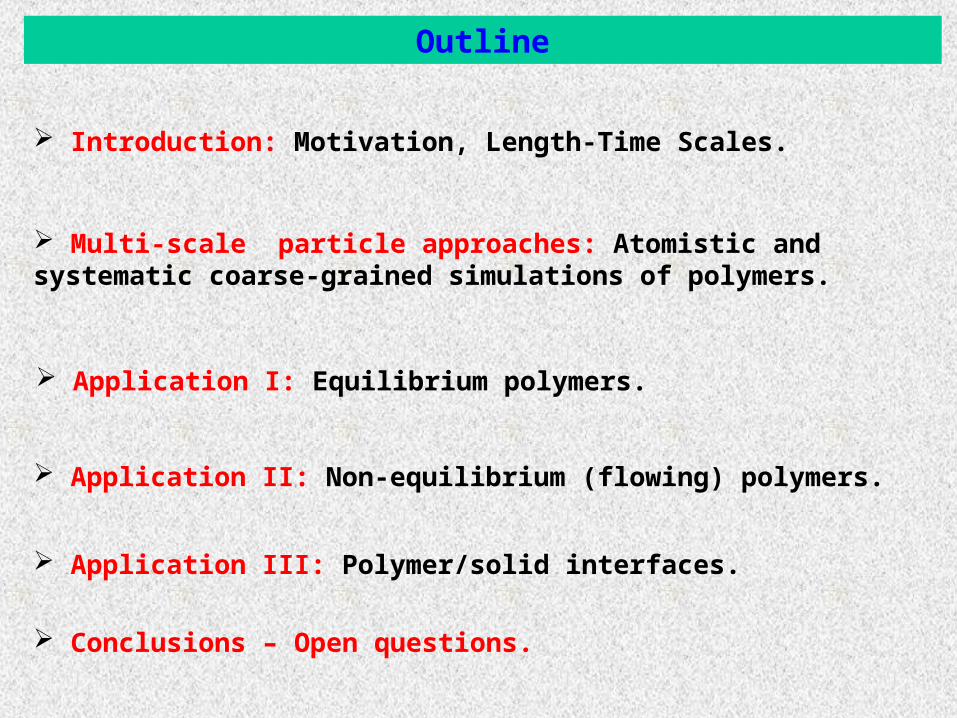
Outline

Introduction: Motivation, Length-Time Scales.

Multi-scale particle approaches: Atomistic and systematic coarse-grained simulations of polymers.

Application I: Equilibrium polymers.

Application II: Non-equilibrium (flowing) polymers.

Conclusions – Open questions.

Application III: Polymer/solid interfaces.

COMPLEX SYSTEMS

-- Broad spectrum of systems, applications, length-time scales.

Systems

-- polymers

-- biological macromolecules (cell membrane, DNA, lipids)-- colloids-- hybrid interfacial systems-- ...

Applications

--- Nanotechnology (materials in nano-dimensions), biotechnology (drug release, … etc)

-- Clever Materials

• Molecular Electronics, Carbon Nanotubes

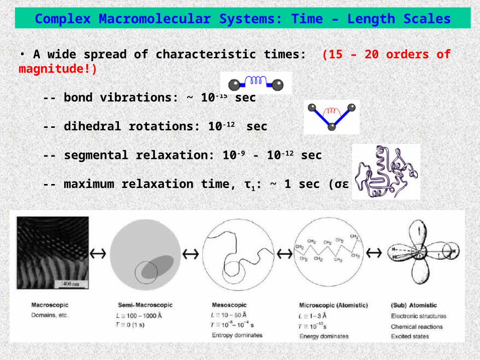
• A wide spread of characteristic times: (15 – 20 orders of magnitude!)

-- bond vibrations: ~ 10-15 sec

-- dihedral rotations: 10-12 sec

-- segmental relaxation: 10-9 - 10-12 sec

-- maximum relaxation time, τ1: ~ 1 sec (σε Τ < Τm)

Complex Macromolecular Systems: Time – Length Scales

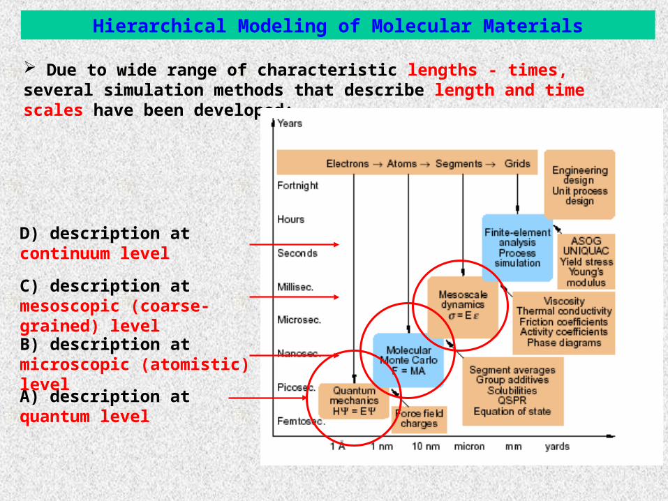
Due to wide range of characteristic lengths - times, several simulation methods that describe length and time scales have been developed:

Α) description at quantum level

Β) description at microscopic (atomistic) level

C) description at mesoscopic (coarse-grained) level

D) description at continuum level

Hierarchical Modeling of Molecular Materials

Molecular Dynamics (MD) [Alder and Wainwright, J. Chem. Phys., 27, 1208 (1957)]

Assume a microscopic (atomistic) system of N interacting particles. Each particle has position ri = (xi,yi, zi). In 3D there are 6N degrees of freedom (3N positions + 3N velocities). Phase space is R6N.

Particles interact with a very complicated and in principle unknown function of 3N variables: U(r1,r2,..., rN).

The time evolution of each particle is (Newton’s eqs. of motion):

21 2

2

( , ,..., )i Ni i

i

d Um

d t

r r r rF

r

Atomistic Molecular Dynamics Method

System of 6N 1st order PDE’s.

1 2( , ,..., )

x ii i

xi N

i

dxp m

dt

dp U

dt x

r r r

N ~ 104 – 105 particles

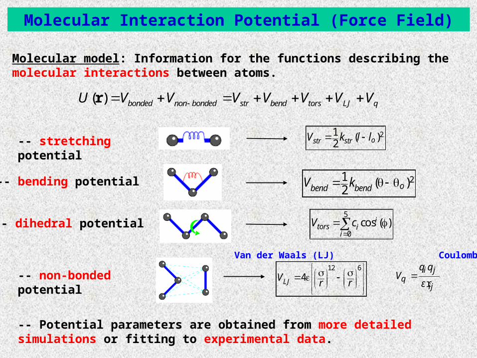
-- Potential parameters are obtained from more detailed simulations or fitting to experimental data.

Molecular model: Information for the functions describing the molecular interactions between atoms.

21 ( )2 obend bendV k -- bending potential

21 ( )2 ostr strV k l l -- stretching potential

-- dihedral potential5

0cos ( )i

tors ii

V c

-- non-bonded potential12 6

4LJVr r

Van der Waals (LJ) Coulomb

ri j

qij

q qV

ε

( ) bonded non bonded str bend tors LJ qU V V V V V V V r

Molecular Interaction Potential (Force Field)

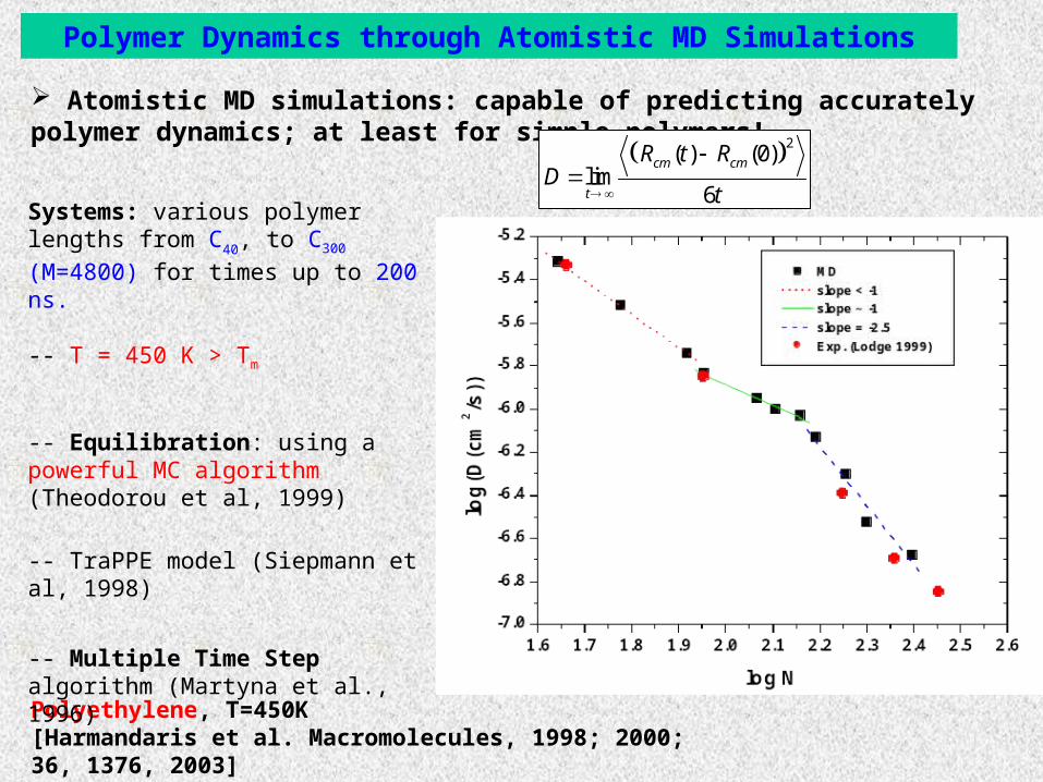
Polymer Dynamics through Atomistic MD Simulations

Atomistic MD simulations: capable of predicting accurately polymer dynamics; at least for simple polymers!

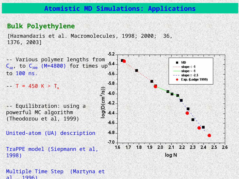
Polyethylene, T=450K[Harmandaris et al. Macromolecules, 1998; 2000; 36, 1376, 2003]

2( ) (0)

lim6

cm cm

t

R t RD

t

Systems: various polymer lengths from C40, to C300 (M=4800) for times up to 200

ns.

-- T = 450 K > Tm

-- Equilibration: using a powerful MC algorithm (Theodorou et al, 1999)

-- TraPPE model (Siepmann et al, 1998)

-- Multiple Time Step algorithm (Martyna et al., 1996)

MULTI-SCALE MODELING OF COMPLEX SYSTEMS

Limits of Atomistic MD Simulations (with usual computer power):

-- Length scale: few Å – O(10 nm)-- Time scale: few fs - O(1 μs) (10-15 – 10-6 sec) ~ 107 – 109 time steps

-- Molecular Length scale (concerning the global dynamics):up to a few Ne for “simple” polymers like PE, PBmuch below Ne for more complicated polymers (like PS)

Need:- Simulations in larger length – time scales.

- Application in molecular weights relevant to polymer processing.

One solution:- Coarse-grained particle models obtained directly from the chemistry.

Atomistic MD Simulations: Allows for quantitative predictions (real numbers!) of the dynamics in soft matter.

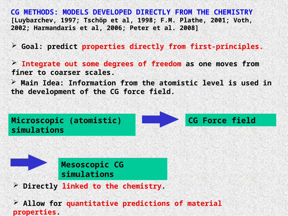
CG METHODS: MODELS DEVELOPED DIRECTLY FROM THE CHEMISTRY[Luybarchev, 1997; Tschöp et al, 1998; F.M. Plathe, 2001; Voth, 2002; Harmandaris et al, 2006; Peter et al. 2008]

Directly linked to the chemistry.

Allow for quantitative predictions of material properties.

Microscopic (atomistic) simulations

CG Force field

Mesoscopic CG simulations

Main Idea: Information from the atomistic level is used in the development of the CG force field.

Goal: predict properties directly from first-principles.

Integrate out some degrees of freedom as one moves from finer to coarser scales.

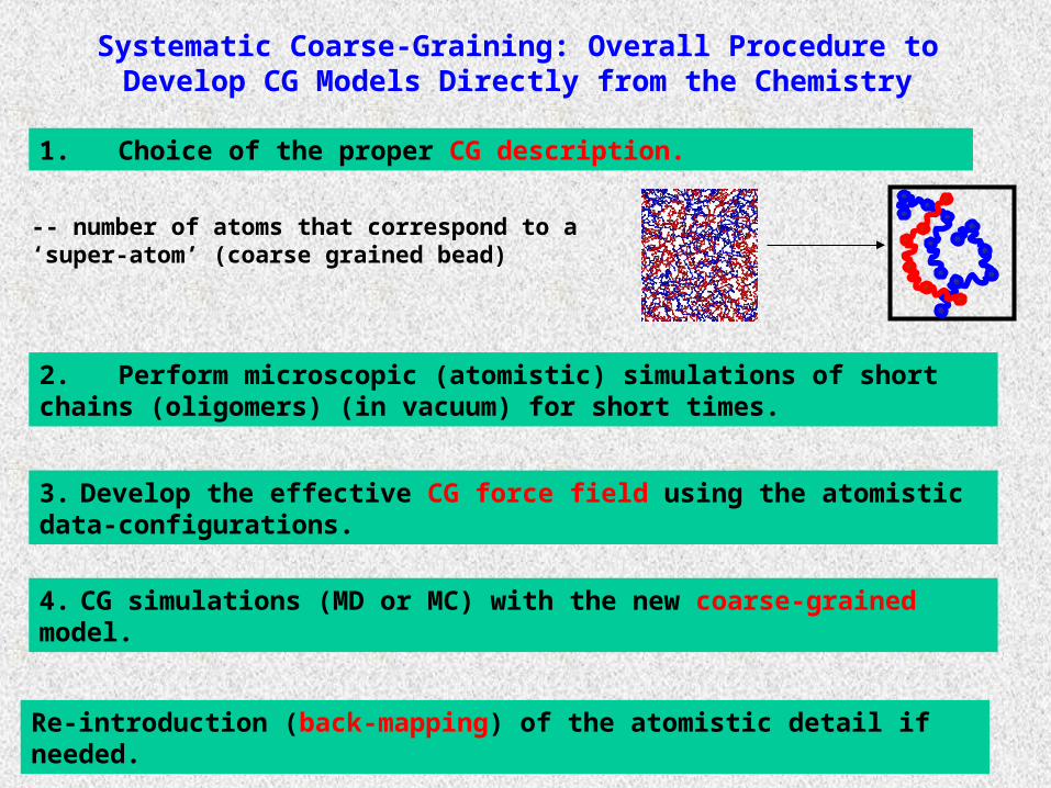
Systematic Coarse-Graining: Overall Procedure to Develop CG Models Directly from the Chemistry

1. Choice of the proper CG description.

2. Perform microscopic (atomistic) simulations of short chains (oligomers) (in vacuum) for short times.

-- number of atoms that correspond to a ‘super-atom’ (coarse grained bead)

3. Develop the effective CG force field using the atomistic data-configurations.

4. CG simulations (MD or MC) with the new coarse-grained model.

Re-introduction (back-mapping) of the atomistic detail if needed.

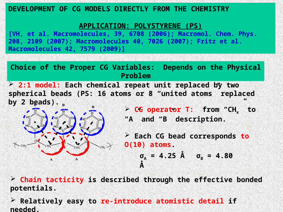
2:1 model: Each chemical repeat unit replaced by two spherical beads (PS: 16 atoms or 8 “united atoms” replaced by 2 beads).

σΑ = 4.25 Å σB = 4.80 Å

Choice of the Proper CG Variables: Depends on the Physical Problem

Chain tacticity is described through the effective bonded potentials.

Relatively easy to re-introduce atomistic detail if needed.

DEVELOPMENT OF CG MODELS DIRECTLY FROM THE CHEMISTRY

APPLICATION: POLYSTYRENE (PS)[VH, et al. Macromolecules, 39, 6708 (2006); Macromol. Chem. Phys. 208, 2109 (2007); Macromolecules 40, 7026 (2007); Fritz et al. Macromolecules 42, 7579 (2009)]

CG operator T: from “CHx” to “A” and “B” description.

Each CG bead corresponds to O(10) atoms.

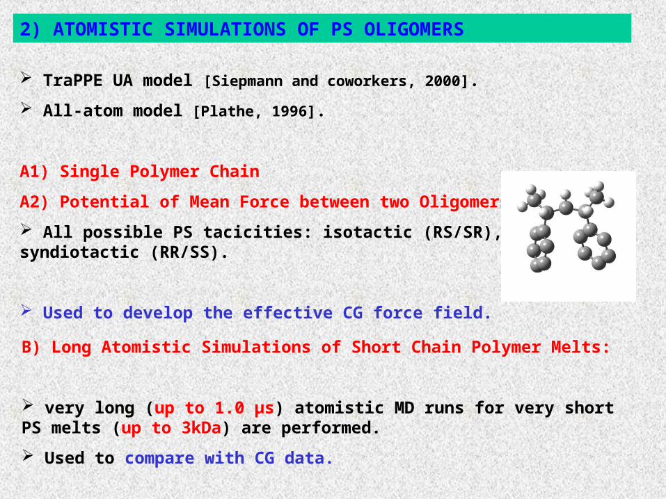
TraPPE UA model [Siepmann and coworkers, 2000].

All-atom model [Plathe, 1996].

A1) Single Polymer Chain

A2) Potential of Mean Force between two Oligomers

All possible PS tacicities: isotactic (RS/SR), syndiotactic (RR/SS).

Used to develop the effective CG force field.

2) ATOMISTIC SIMULATIONS OF PS OLIGOMERS

B) Long Atomistic Simulations of Short Chain Polymer Melts:

very long (up to 1.0 μs) atomistic MD runs for very short PS melts (up to 3kDa) are performed.

Used to compare with CG data.

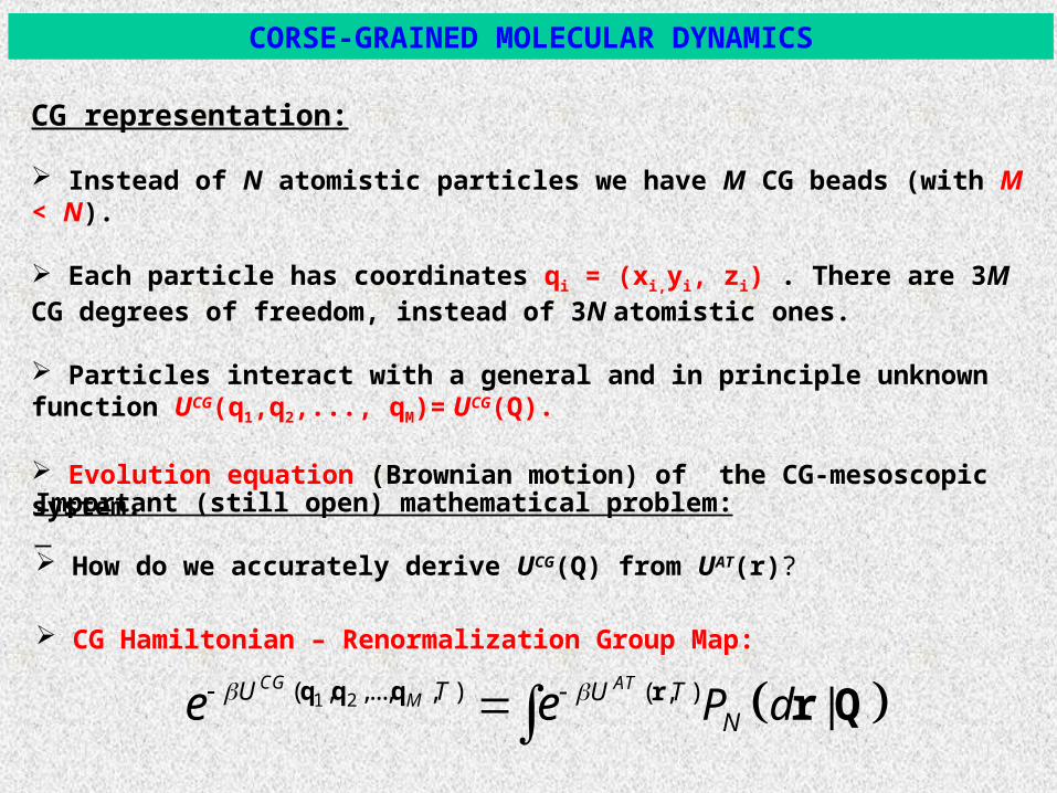
CG representation:

Instead of N atomistic particles we have M CG beads (with M < N).

Each particle has coordinates qi = (xi,yi, zi) . There are 3M CG degrees of freedom, instead of 3N atomistic ones.

Particles interact with a general and in principle unknown function UCG(q1,q2,..., qM)= UCG(Q).

Evolution equation (Brownian motion) of the CG-mesoscopic system.

CORSE-GRAINED MOLECULAR DYNAMICS

CG Hamiltonian – Renormalization Group Map:

1 2( , ,..., , ) ( , ) |CG AT

MU T U TNP de e q q q r r Q

Important (still open) mathematical problem: How do we accurately derive UCG(Q) from UAT(r)?

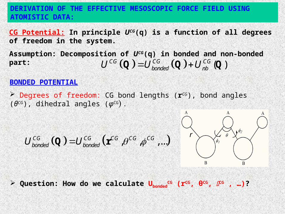
DERIVATION OF THE EFFECTIVE MESOSCOPIC FORCE FIELD USING ATOMISTIC DATA:

r

BONDED POTENTIAL

Degrees of freedom: CG bond lengths (rCG), bond angles (θCG), dihedral angles (φCG).

( )CG CG CGbonded nbU U U Q Q Q

CG Potential: In principle UCG(q) is a function of all degrees of freedom in the system.

Assumption: Decomposition of UCG(q) in bonded and non-bonded part:

, , ,...CG CG CG CG CGbonded bondedU U Q r

Question: How do we calculate UbondedCG (rCG, θCG, CG , …)?

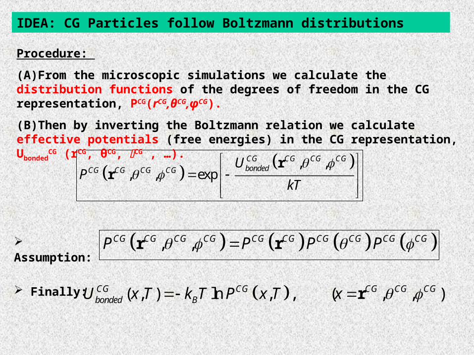
IDEA: CG Particles follow Boltzmann distributions

, ,, , exp

CG CG CG CGbondedCG CG CG CG

UP

kT

rr

Assumption:

( , ) ln , , ( , , )CG CG CG CG CGbonded BU x T k T P x T x r

, ,CG CG CG CG CG CG CG CG CG CGP P P P r r

Finally:

Procedure:

(A)From the microscopic simulations we calculate the distribution functions of the degrees of freedom in the CG representation, PCG(rCG,θCG,φCG).

(B)Then by inverting the Boltzmann relation we calculate effective potentials (free energies) in the CG representation, Ubonded

CG (rCG, θCG, CG , …).

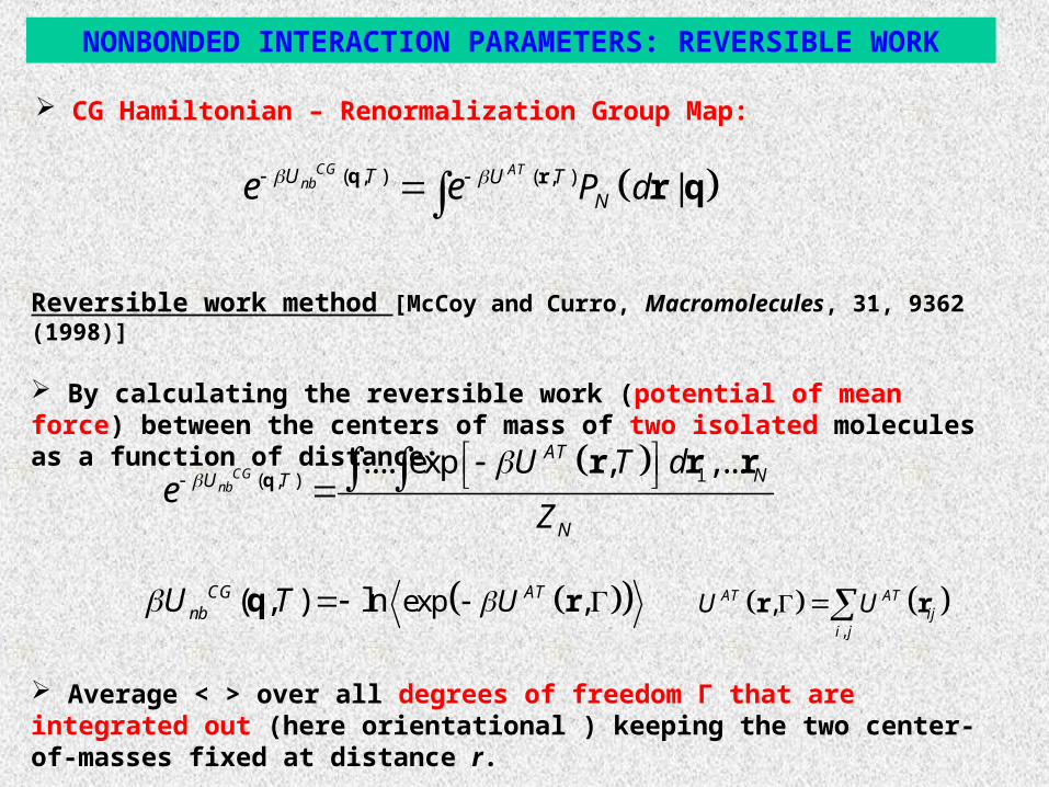
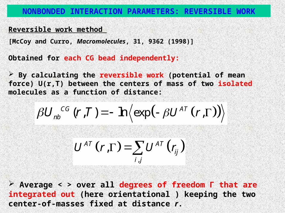
NONBONDED INTERACTION PARAMETERS: REVERSIBLE WORK

Reversible work method [McCoy and Curro, Macromolecules, 31, 9362 (1998)]

By calculating the reversible work (potential of mean force) between the centers of mass of two isolated molecules as a function of distance:

exp ,( , ) lnCG ATnb UU T rq

,

,AT ATij

i j

U U r r

Average < > over all degrees of freedom Γ that are integrated out (here orientational ) keeping the two center-of-masses fixed at distance r.

1( , ).... exp , ,...CG

nb

ATNU T

N

U T d

Ze

qr r r

CG Hamiltonian – Renormalization Group Map:

( , ) ( , ) |CG AT

nbU T U TNP de e q r r q

q

Solution: Use of conditional reversible work[Fritz et al, 2009; E. Brini et al. 2011]

Main assumptions: (A) Neglect many-body effect. Exact for the gas phase.(B) Chain effect is not described. In our case CG particles belong to a

macromolecule.


Calculate “reversible work” using a numerical method (eg. MC or MD).

,( , ) ( , ) ( , )CG AB A B Exclnb PMF PMFU T V T V T q q q

Main idea: Use instead two very short chains and keep constant the distance between the center-of-mass of only the two target CG (e.g. A, B) particles.

(A) Calculate the PMF including all atomistic interactions, (B) Calculate the PMF with all atomistic interactions excluding the A-B ones.

( , )ABPMFV Tq

, ( , )A B ExclPMFV T q

Effective CG interaction is:

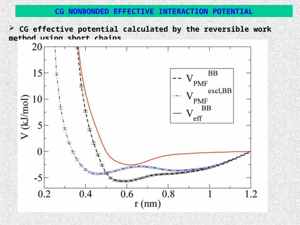
CG effective potential calculated by the reversible work method using short chains.

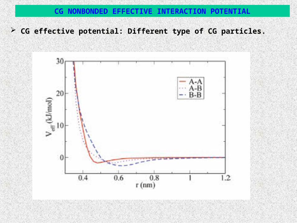
CG NONBONDED EFFECTIVE INTERACTION POTENTIAL

System: Atactic PS melts with molecular length from 1kDa (10 monomers) up to 10kDa (1kDa = 1000 gr/mol, T=463K).

Method: MD with a Langevin thermostat

2

2 ( )CG

ii i

ii

W tU

mt t

q qq

4) CG MOLECULAR DYNAMICS SIMULATIONS

Friction Force: with friction coefficient Γ = 1.0/τ

Random force:(fluctuation-dissipation theorem)

( ) ( ) 6i j ij BW t W t t t k T g

m

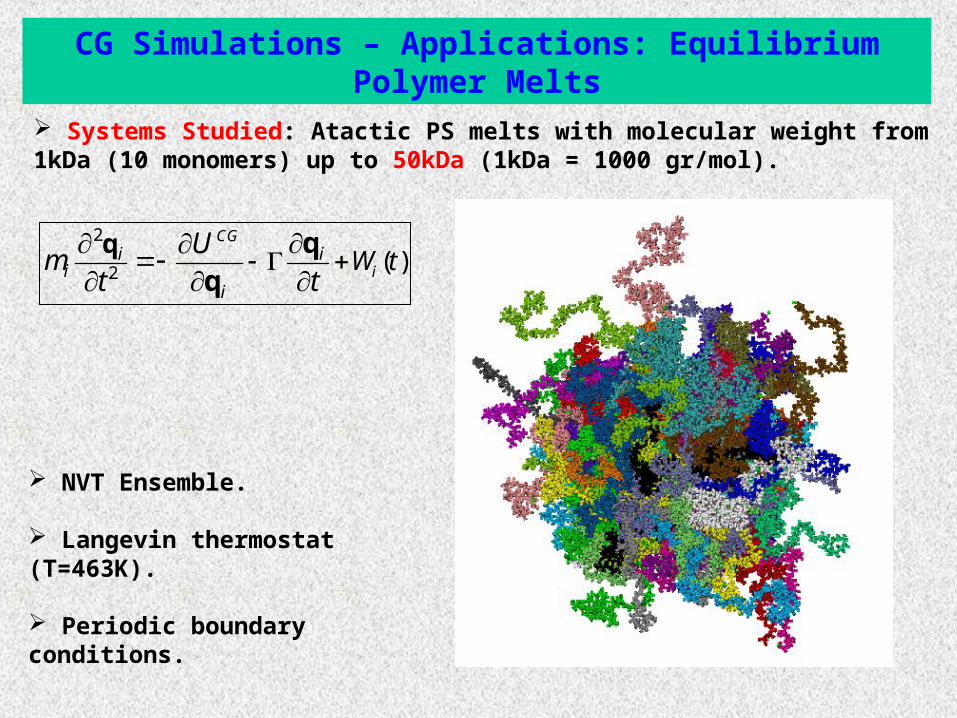
Systems Studied: Atactic PS melts with molecular weight from 1kDa (10 monomers) up to 50kDa (1kDa = 1000 gr/mol).

CG Simulations – Applications: Equilibrium Polymer Melts

NVT Ensemble.

Langevin thermostat (T=463K).

Periodic boundary conditions.

2

2 ( )CG

ii i

ii

W tU

mt t

q qq

BACK-MAPPING PROCEDURE: FROM MESOSCOPIC DESCRIPTION TO ATOMISTIC DETAIL

Goal: from the CG configuration obtain a microscopic one.

-- In many cases we need microscopic configuration.

No unique solution !! Note: One CG configuration corresponds to many microscopic ones

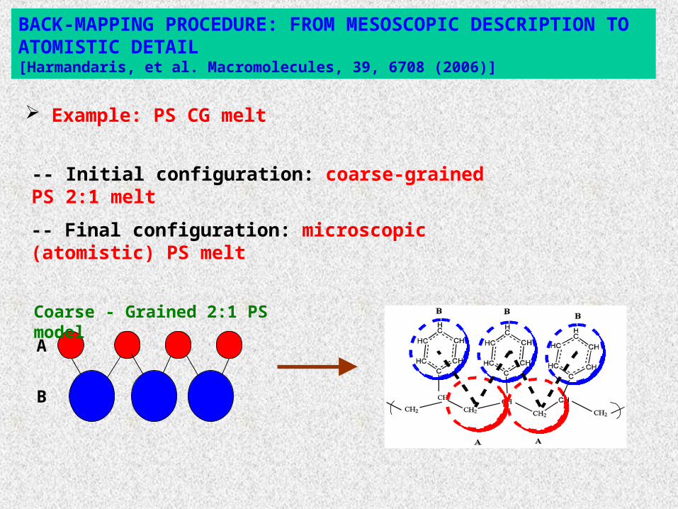
BACK-MAPPING PROCEDURE: FROM MESOSCOPIC DESCRIPTION TO ATOMISTIC DETAIL[Harmandaris, et al. Macromolecules, 39, 6708 (2006)]

-- Initial configuration: coarse-grained PS 2:1 melt

A

B

Coarse - Grained 2:1 PS model

Example: PS CG melt

-- Final configuration: microscopic (atomistic) PS melt

BACK-MAPPING PROCEDURE: FROM MESOSCOPIC DESCRIPTION TO ATOMISTIC DETAIL[Harmandaris, et al. Macromolecules, 39, 6708 (2006)]

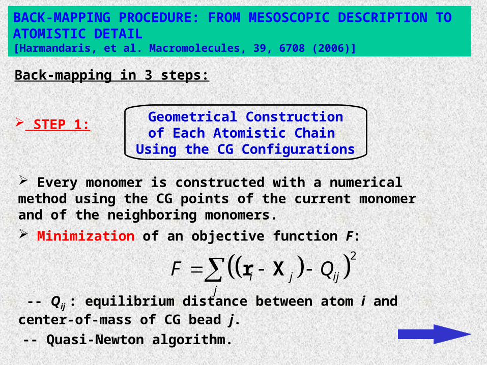
Geometrical Constructionof Each Atomistic Chain

Using the CG Configurations

Back-mapping in 3 steps:

STEP 1:

Every monomer is constructed with a numerical method using the CG points of the current monomer and of the neighboring monomers.

2

i j ijj

F Q r X

Minimization of an objective function F:

-- Qij : equilibrium distance between atom i and center-of-mass of CG bead j.

-- Quasi-Newton algorithm.

Total Energy Minimization Scheme

Very Short (~20 ps) MD Run to Obtain Realistic

Configurations

STEP 2:

BACK-MAPPING PROCEDURE: FROM MESOSCOPIC DESCRIPTION TO ATOMISTIC DETAIL

STEP 3:

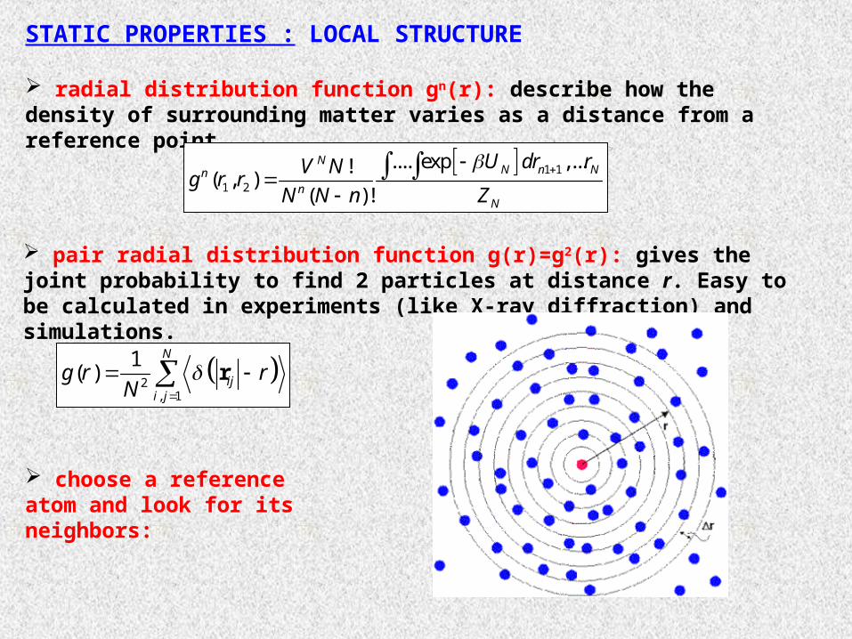
STATIC PROPERTIES : LOCAL STRUCTURE

radial distribution function gn(r): describe how the density of surrounding matter varies as a distance from a reference point.

pair radial distribution function g(r)=g2(r): gives the joint probability to find 2 particles at distance r. Easy to be calculated in experiments (like X-ray diffraction) and simulations.

1 1

1 2

.... exp ,...!( , )

( )!

NN n Nn

nN

U dr rV Ng r r

N N n Z

2, 1

1( )

N

iji j

g r rN

r

choose a reference atom and look for its neighbors:

Compare structure in atomistic configurations (of a 1kDa system) obtained from:

Very long (0.5 μs) “pure” atomistic MD runs.

Short-fast CG MD runs: reinsertion of the atomistic detail in CG configurations.

Intramolecular g(r)

VALIDATION OF THE BACK-MAPPING PROCEDURE

Intermolecular CH2 – CH2 g(r)

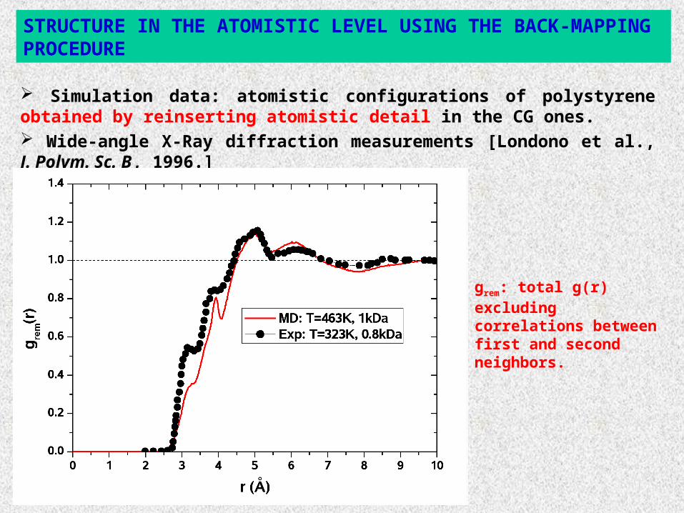
Simulation data: atomistic configurations of polystyrene obtained by reinserting atomistic detail in the CG ones. Wide-angle X-Ray diffraction measurements [Londono et al., J. Polym. Sc. B, 1996.]

STRUCTURE IN THE ATOMISTIC LEVEL USING THE BACK-MAPPING PROCEDURE

grem: total g(r) excluding correlations between first and second neighbors.

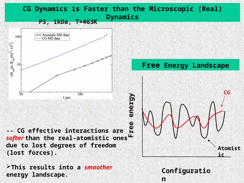
CG Dynamics is Faster than the Microscopic (Real) Dynamics

PS, 1kDa, T=463K

Free Energy Landscape

-- CG effective interactions are softer than the real-atomistic ones due to lost degrees of freedom (lost forces).

This results into a smoother energy landscape.

Configuration

Fre

e en

ergy

Atomistic

CG

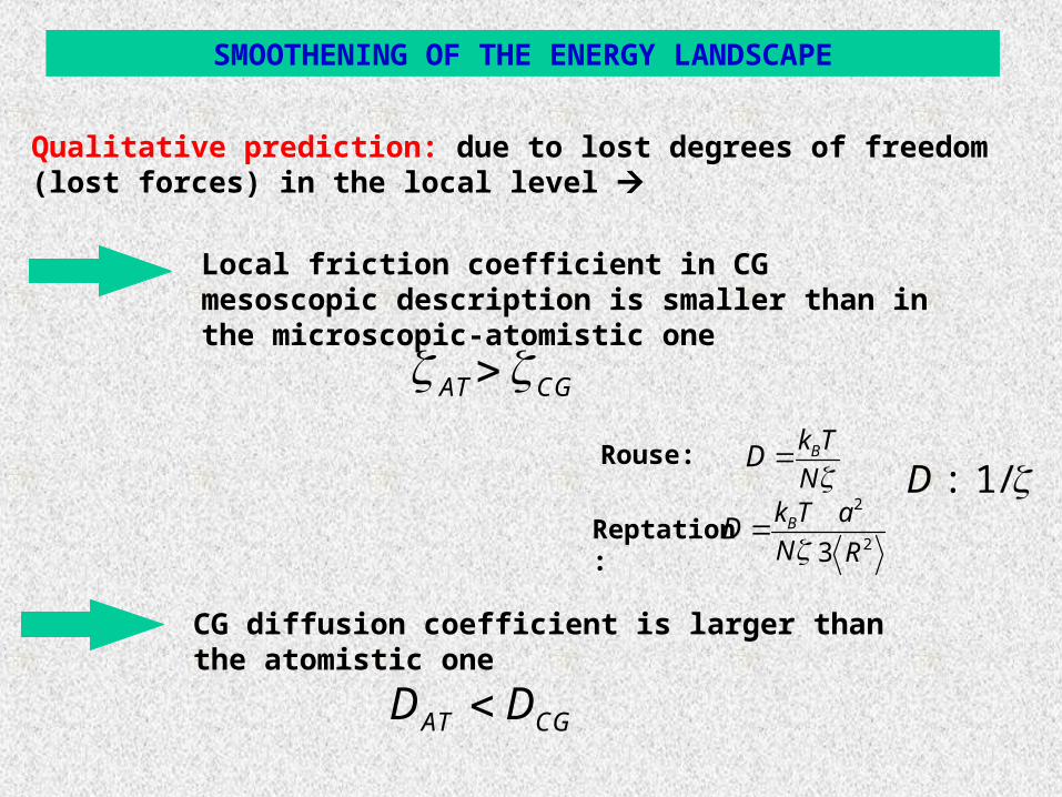
Qualitative prediction: due to lost degrees of freedom (lost forces) in the local level

Local friction coefficient in CG mesoscopic description is smaller than in the microscopic-atomistic one

SMOOTHENING OF THE ENERGY LANDSCAPE

AT CG

CG diffusion coefficient is larger than the atomistic one

AT CGD D

Bk T

ND

Rouse:

2

23 Bk T a

N RD

Reptation:

1/D :

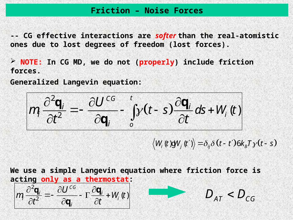
Friction – Noise Forces

-- CG effective interactions are softer than the real-atomistic ones due to lost degrees of freedom (lost forces).

NOTE: In CG MD, we do not (properly) include friction forces.

Generalized Langevin equation:

2

2 ( )tCG

i

o

i ii

i

t s ds W tU

mt t

q qq

We use a simple Langevin equation where friction force is acting only as a thermostat:

2

2 ( )CG

ii i

ii

W tU

mt t

q qq

( ) ( ) 6i j ij BW t W t t t k T t s g

AT CGD D

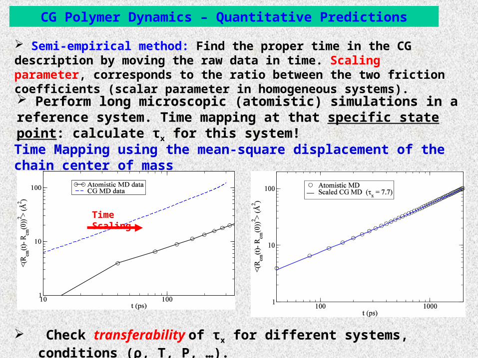
CG Polymer Dynamics – Quantitative Predictions

Perform long microscopic (atomistic) simulations in a reference system. Time mapping at that specific state point: calculate τx for this system!

Check transferability of τx for different systems, conditions (ρ, T, P, …).

Time Scaling

Semi-empirical method: Find the proper time in the CG description by moving the raw data in time. Scaling parameter, corresponds to the ratio between the two friction coefficients (scalar parameter in homogeneous systems).

Time Mapping using the mean-square displacement of the chain center of mass

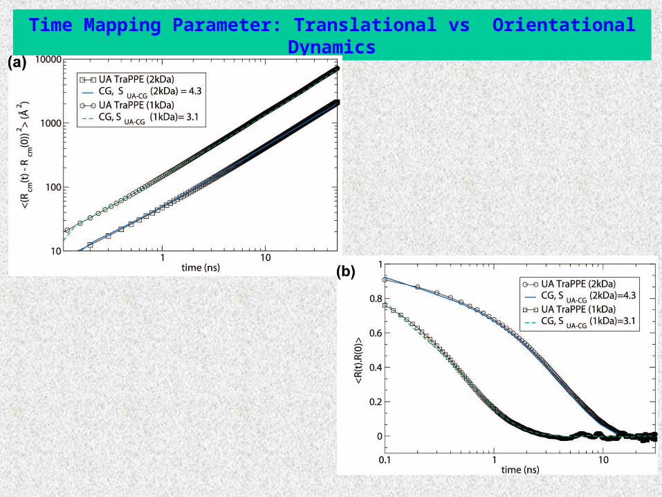
Time Mapping Parameter: Translational vs Orientational Dynamics

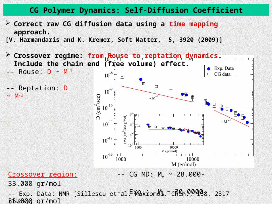
CG Polymer Dynamics: Self-Diffusion Coefficient

-- Exp. Data: NMR [Sillescu et al. Makromol. Chem., 188, 2317 (1987)]

-- Rouse: D ~ M-1

-- Reptation: D ~ M-2

Crossover region: -- CG MD: Me ~ 28.000-33.000 gr/mol -- Exp.: Me ~ 30.0000-35.000 gr/mol

Correct raw CG diffusion data using a time mapping approach.[V. Harmandaris and K. Kremer, Soft Matter, 5, 3920 (2009)]

Crossover regime: from Rouse to reptation dynamics. Include the chain end (free volume) effect.

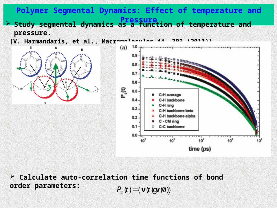
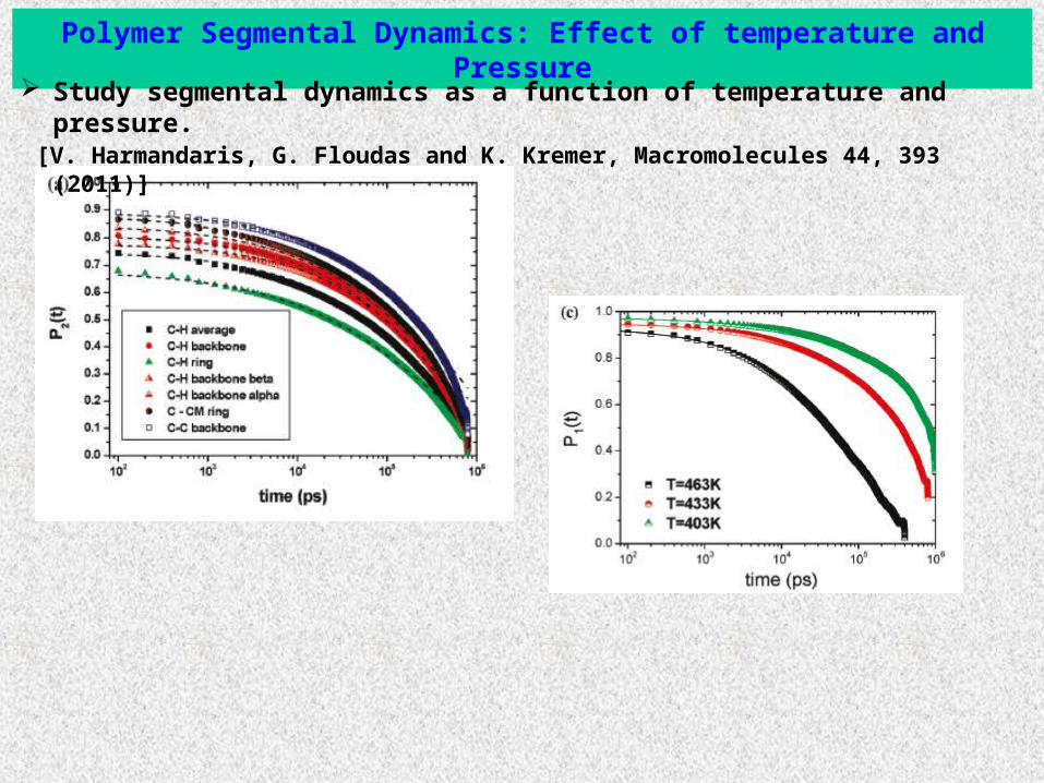
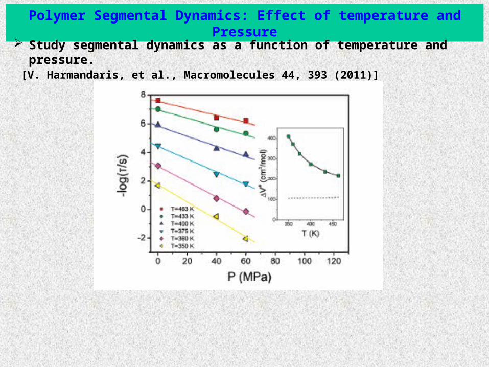
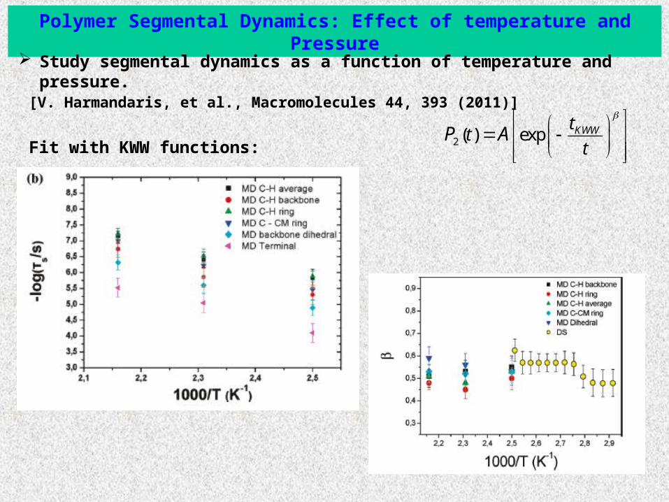
Polymer Segmental Dynamics: Effect of temperature and Pressure

Study segmental dynamics as a function of temperature and pressure. [V. Harmandaris, et al., Macromolecules 44, 393 (2011)]

Calculate auto-correlation time functions of bond order parameters:

2 ( ) ( ) (0)t tP v vg


Get segmental relaxation times from MD simulations: Compare directly with dielectric experiments.

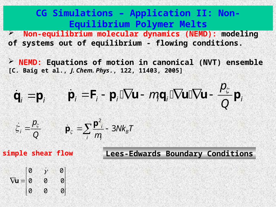
Non-equilibrium molecular dynamics (NEMD): modeling of systems out of equilibrium - flowing conditions.

CG Simulations – Application II: Non-Equilibrium Polymer Melts

i iq p i i i i i i

pm

Q p F p u q u u p

i

p

Q

2

3iB

i i

Nk Tm p

p

0 0

0 0 0

0 0 0

u

NEMD: Equations of motion in canonical (NVT) ensemble[C. Baig et al., J. Chem. Phys., 122, 11403, 2005]

simple shear flow Lees-Edwards Boundary Conditions

Primary

L

L

y

ux

x

y

x

ux

tL

Lees-Edwards Boundary Conditions

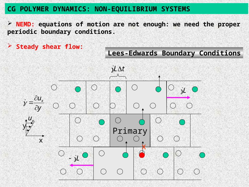
CG POLYMER DYNAMICS: NON-EQUILIBRIUM SYSTEMS

NEMD: equations of motion are not enough: we need the proper periodic boundary conditions.

Steady shear flow:

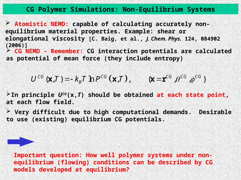
CG Polymer Simulations: Non-Equilibrium Systems

CG NEMD - Remember: CG interaction potentials are calculated as potential of mean force (they include entropy).

In principle UCG(x,T) should be obtained at each state point, at each flow field.

Important question: How well polymer systems under non-equilibrium (flowing) conditions can be described by CG models developed at equilibrium?

Idea: Use an existing equilibrium CG polymer model under non-equilibrium conditions.

Direct comparison between atomistic and CG NEMD simulations for various flow fields. Strength of flow (Weissenberg number, Wi = 0.3 - 200) Wi

Short atactic PS melts (M=2kDa, 20 monomers) are studied by both atomistic and CG NEMD simulations.

( , ) ln , , ( , , )CG CG CG CG CGbonded BU x T k T P x T x r

CG Non-Equilibrium Polymers: Conformations

2

3

eq

R Rc

R

Wi Properties as a function of strength of flow (Weissenberg number)

Conformation tensor:

Atomistic cxx: asymptotic behavior at high Wi because of (a) finite chain extensibility, (b) chain rotation during shear flow.

CG cxx: allows for larger maximum chain extension at high Wi because of the softer interaction potentials.

-- R is the end-to-end vector

CG Non-Equilibrium Polymers: Conformation Tensor

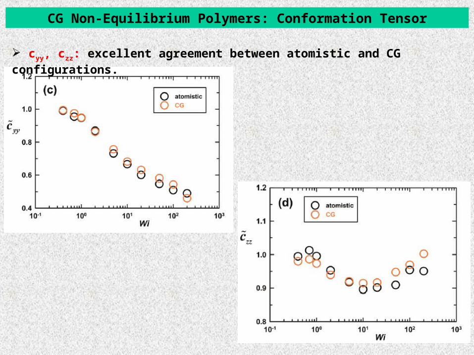
cyy, czz: excellent agreement between atomistic and CG configurations.

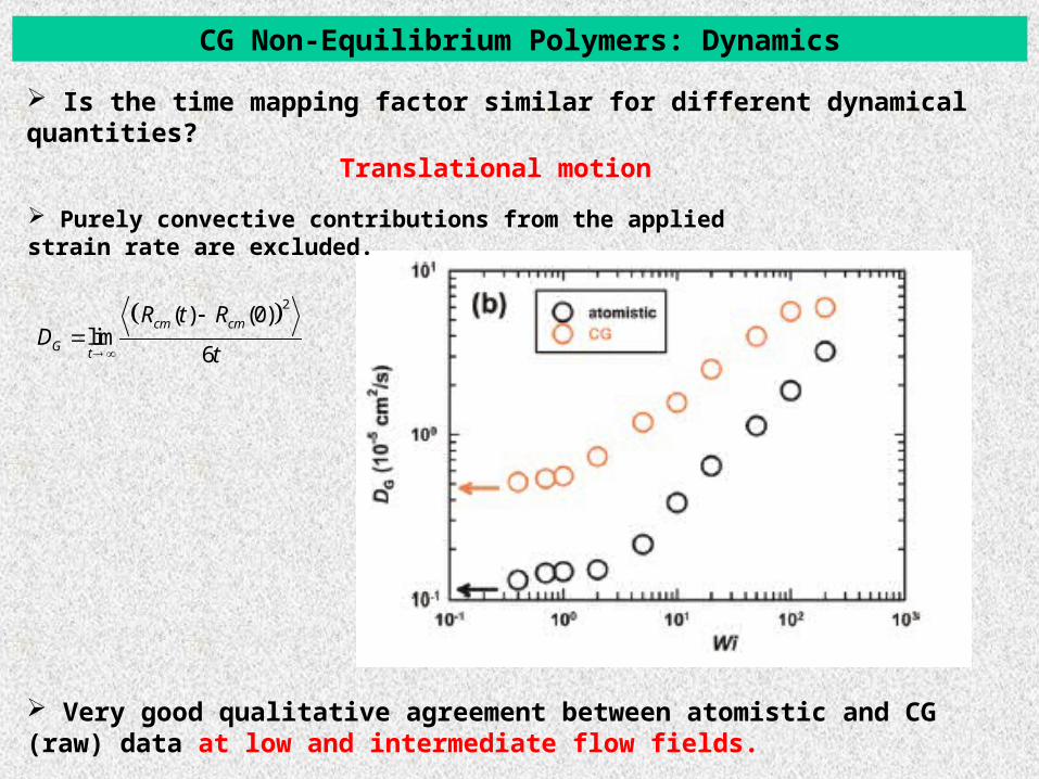
CG Non-Equilibrium Polymers: Dynamics

Translational motion

2( ) (0)

lim6

cm cm

G t

R t RD

t

Is the time mapping factor similar for different dynamical quantities?

Very good qualitative agreement between atomistic and CG (raw) data at low and intermediate flow fields.

Purely convective contributions from the applied strain rate are excluded.


Orientational motion

2( ) (0) ( ) expeq

r

tR t R R t

Rotational relaxation time: small variations at low strain rates, large decrease at high flow fields.

Good agreement between atomistic and CG at low and intermediate flow fields.


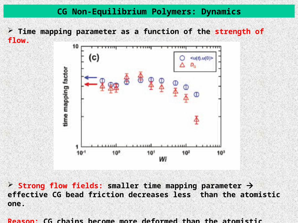
Time mapping parameter as a function of the strength of flow.

Strong flow fields: smaller time mapping parameter effective CG bead friction decreases less than the atomistic one.

Reason: CG chains become more deformed than the atomistic ones.

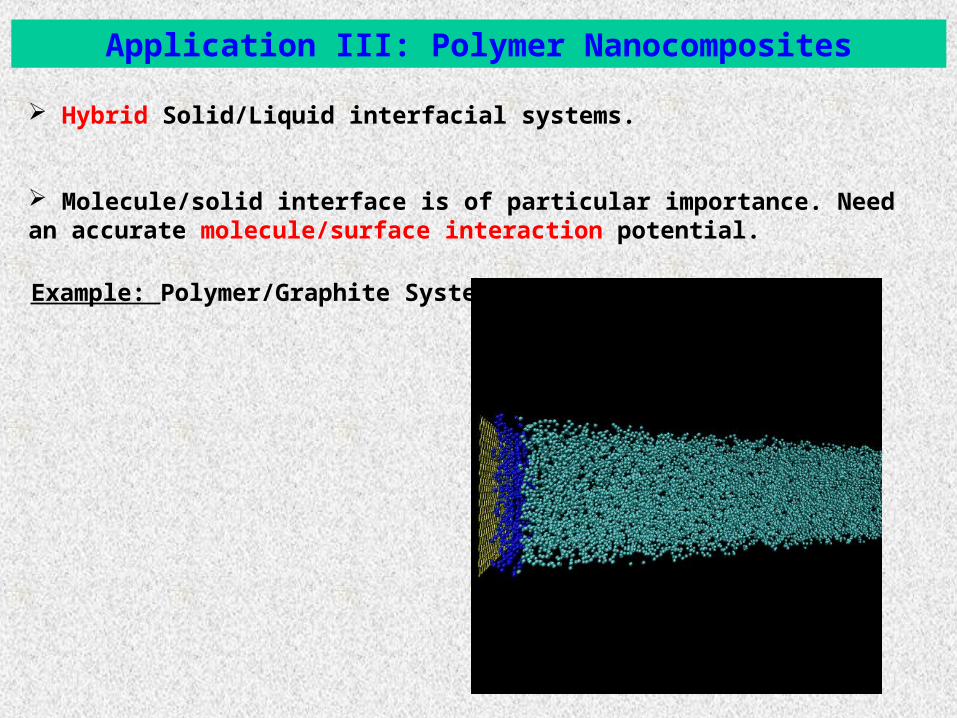
Hybrid Solid/Liquid interfacial systems.

Molecule/solid interface is of particular importance. Need an accurate molecule/surface interaction potential.

Application III: Polymer Nanocomposites

Example: Polymer/Graphite System.

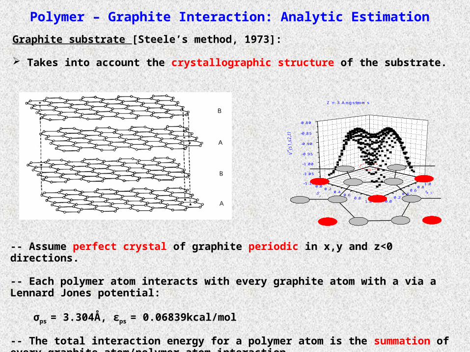
Graphite substrate [Steele’s method, 1973]:

Takes into account the crystallographic structure of the substrate.

-- Assume perfect crystal of graphite periodic in x,y and z<0 directions.

-- Each polymer atom interacts with every graphite atom with a via a Lennard Jones potential:

σps = 3.304Å, εps = 0.06839kcal/mol

-- The total interaction energy for a polymer atom is the summation of every graphite atom/polymer atom interaction.

0.00.2

0.40.6

0.81.0

-1.10

-1.05

-1.00

-0.95

-0.90

-0.85

-0.80

0.00.2

0.40.6

0.81.0

Z = 3 Angstroms

Polymer – Graphite Interaction: Analytic Estimation

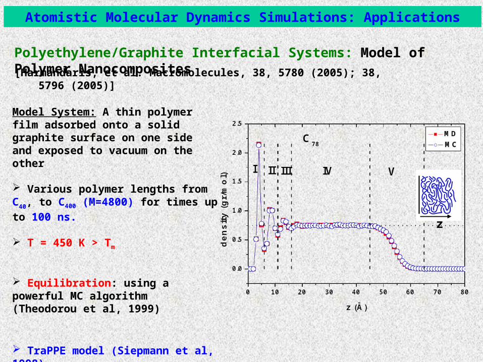
Polyethylene/Graphite Interfacial Systems: Model of Polymer Nanocomposites

Atomistic Molecular Dynamics Simulations: Applications

Model System: A thin polymer film adsorbed onto a solid graphite surface on one side and exposed to vacuum on the other

Various polymer lengths from C40, to C400

(M=4800) for times up to 100 ns.

T = 450 K > Tm

Equilibration: using a powerful MC algorithm (Theodorou et al, 1999)

TraPPE model (Siepmann et al, 1998)Multiple Time Step (Martyna et al., 1996)

[Harmandaris, et al. Macromolecules, 38, 5780 (2005); 38, 5796 (2005)]

z

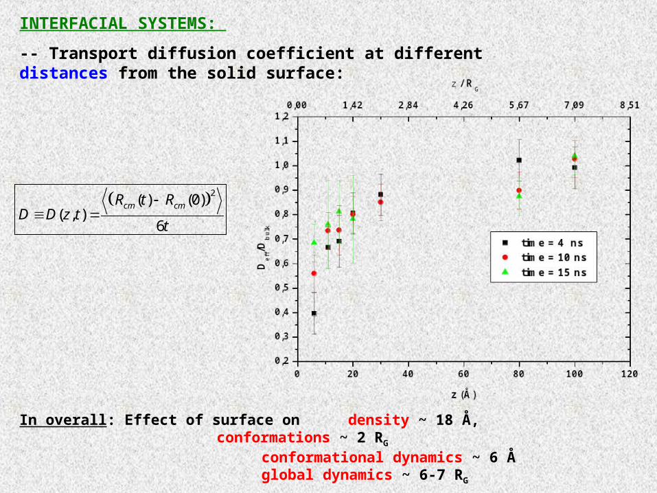
INTERFACIAL SYSTEMS:

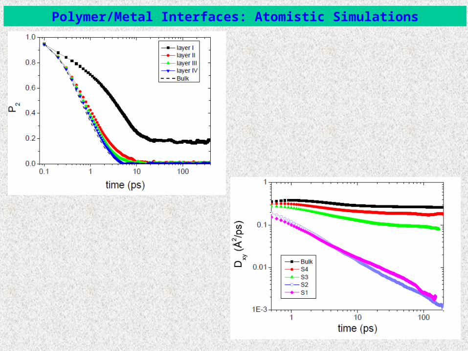
-- Transport diffusion coefficient at different distances from the solid surface:

In overall: Effect of surface on density ~ 18 Å,conformations ~ 2 RG

conformational dynamics ~ 6 Åglobal dynamics ~ 6-7 RG

2( ) (0)

( , )6

cm cmR t RD D z t

t

Test example: Benzene/Au systems

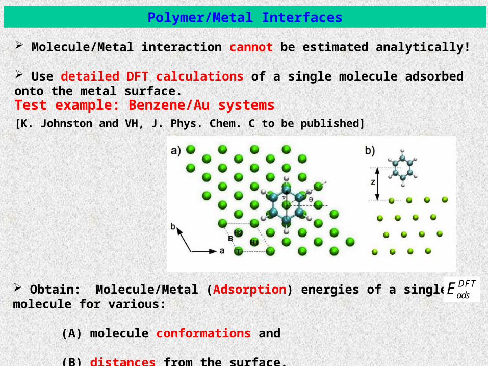
Polymer/Metal Interfaces

[K. Johnston and VH, J. Phys. Chem. C to be published]

Molecule/Metal interaction cannot be estimated analytically!

Use detailed DFT calculations of a single molecule adsorbed onto the metal surface.

Obtain: Molecule/Metal (Adsorption) energies of a single molecule for various:

(A) molecule conformations and

(B) distances from the surface.

DFTadsE

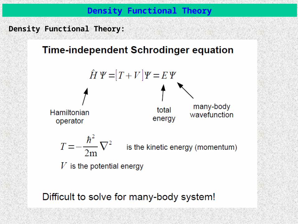
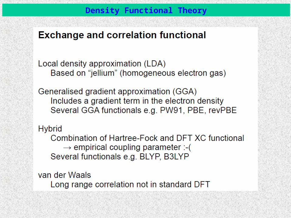
Density Functional Theory

Density Functional Theory:

Density Functional Theory

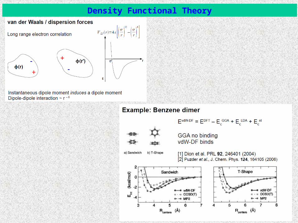
Benzene/Au systems: Density Functional Theory

Adsorption sites, angles, distances and energy for a single benzene molecule:

DFTadsE

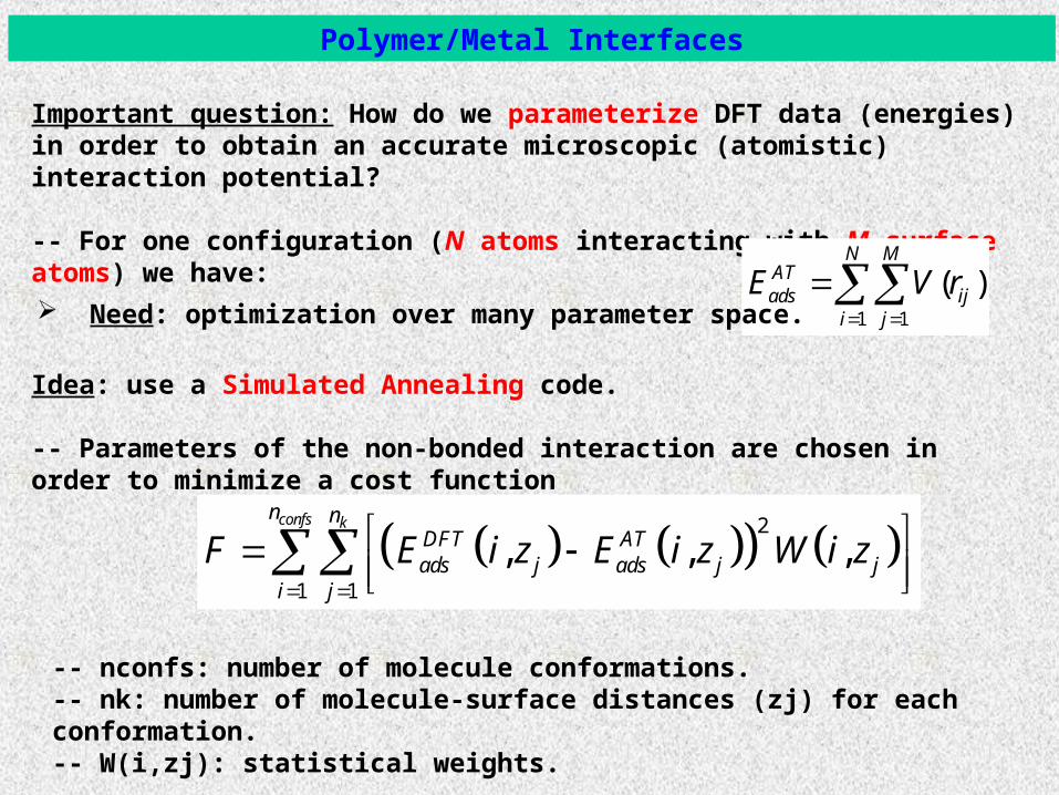
Important question: How do we parameterize DFT data (energies) in order to obtain an accurate microscopic (atomistic) interaction potential?

-- For one configuration (N atoms interacting with M surface atoms) we have:

Polymer/Metal Interfaces

Idea: use a Simulated Annealing code.

-- Parameters of the non-bonded interaction are chosen in order to minimize a cost function

2

1 1

, , ,confs k

n nDFT ATads j ads j j

i j

F E i z E i z W i z

-- nconfs: number of molecule conformations.-- nk: number of molecule-surface distances (zj) for each conformation.-- W(i,zj): statistical weights.

1 1

( )N M

ATads ij

i j

E V r

Need: optimization over many parameter space.

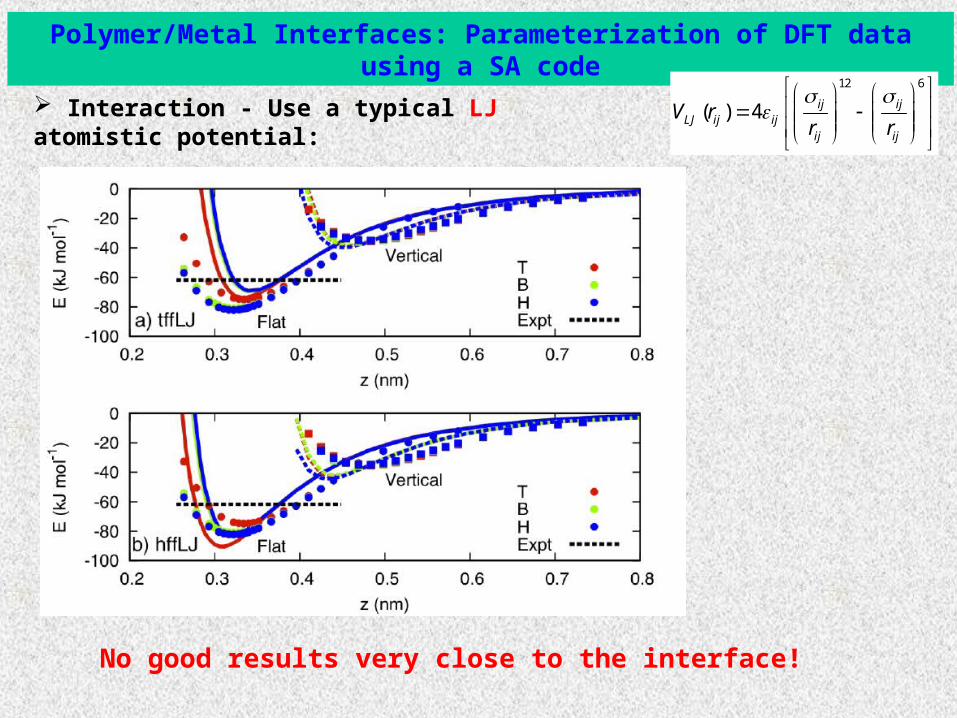
Polymer/Metal Interfaces: Parameterization of DFT data using a SA code

Interaction - Use a typical LJ atomistic potential:12 6

( ) 4 ij ijLJ ij ij

ij ij

V rr r

No good results very close to the interface!

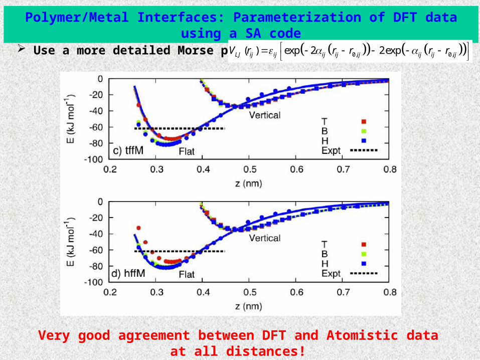
Polymer/Metal Interfaces: Parameterization of DFT data using a SA code

Use a more detailed Morse potential: 0, 0,( ) exp 2 2expLJ ij ij ij ij ij ij ij ijV r r r r r

Very good agreement between DFT and Atomistic data at all distances!

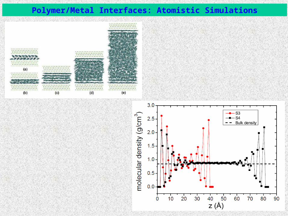
Polymer/Metal Interfaces: Atomistic Simulations

Conclusions Hierarchical systematic CG models, developed from isolated atomistic chains, allow for the good prediction of polymer structure and dimensions.

CG MD: friction forces are not (properly) include, i.e. dynamics is faster but

Time mapping using dynamical information from atomistic description allow for quantitative dynamical predictions from the CG simulations, at least for some cases like homogeneous one component systems.

Overall speed up of the mesoscopic dynamic simulations, compared with the atomistic, is ~ 3-5 orders of magnitude.

Other systems (molecule/polymer blends, …) can also be studied with systematic CC models.

Deviations between atomistic and CG NEMD data at high flow fields.

Molecular systems at non-equilibrium conditions can be accurately studied at low and medium flow fields.

End of the “Good News” ….

Quantitatively inaccurate predictions: -- dynamics, -- phase transitions, -- melt structure, -- crystallization, -- ...

More Conclusions

All the above applications are either qualitative predictions or can be used quantitatively only in small range of states (ρ, T, P, ... etc.)

Make everything as simple as possible but not simpler!

A. Einstein, 1879-1955

Simplicity is theultimate sophistication!

Leonardo da Vinci, 1452-1519

BUT …. What is “simpler” in CG description?

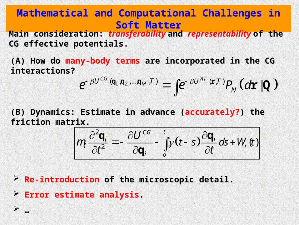
(A) How do many-body terms are incorporated in the CG interactions?

Mathematical and Computational Challenges in Soft Matter

(B) Dynamics: Estimate in advance (accurately?) the friction matrix.

Re-introduction of the microscopic detail.

Error estimate analysis.

…

Main consideration: transferability and representability of the CG effective potentials.

1 2( , ,..., , ) ( , ) |CG AT

MU T U TNP de e q q q r r Q

2

2 ( )tCG

i

o

i ii

i

t s ds W tU

mt t

q qq

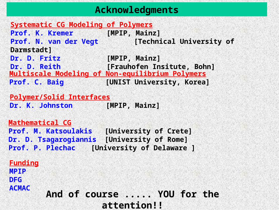
Acknowledgments

Systematic CG Modeling of PolymersProf. K. Kremer [MPIP, Mainz]Prof. N. van der Vegt [Technical University of Darmstadt]Dr. D. Fritz [MPIP, Mainz]Dr. D. Reith [Frauhofen Insitute, Bohn]

FundingMPIPDFGACMAC

Multiscale Modeling of Non-equilibrium PolymersProf. C. Baig [UNIST University, Korea]

And of course ..... YOU for the attention!!

Polymer/Solid InterfacesDr. K. Johnston [MPIP, Mainz]

Mathematical CGProf. M. Katsoulakis [University of Crete]Dr. D. Tsagarogiannis [University of Rome]Prof. P. Plechac [University of Delaware ]

EXTRA SLIDES

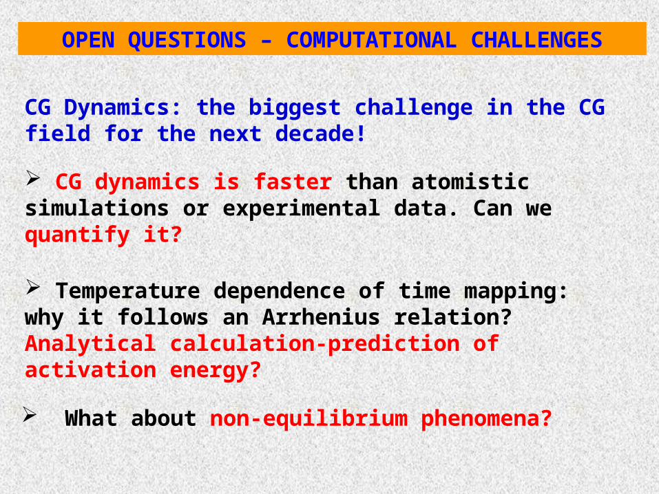
CG dynamics is faster than atomistic simulations or experimental data. Can we quantify it?

Temperature dependence of time mapping: why it follows an Arrhenius relation? Analytical calculation-prediction of activation energy?

OPEN QUESTIONS – COMPUTATIONAL CHALLENGES

CG Dynamics: the biggest challenge in the CG field for the next decade!

What about non-equilibrium phenomena?

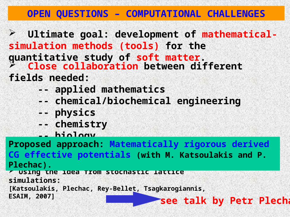
OPEN QUESTIONS – COMPUTATIONAL CHALLENGES

Ultimate goal: development of mathematical-simulation methods (tools) for the quantitative study of soft matter.

Close collaboration between different fields needed:-- applied mathematics-- chemical/biochemical engineering-- physics-- chemistry-- biology

Using the idea from stochastic lattice simulations:[Katsoulakis, Plechac, Rey-Bellet, Tsagkarogiannis, ESAIM, 2007]

Proposed approach: Matematically rigorous derived CG effective potentials (with M. Katsoulakis and P. Plechac).

see talk by Petr Plechac!

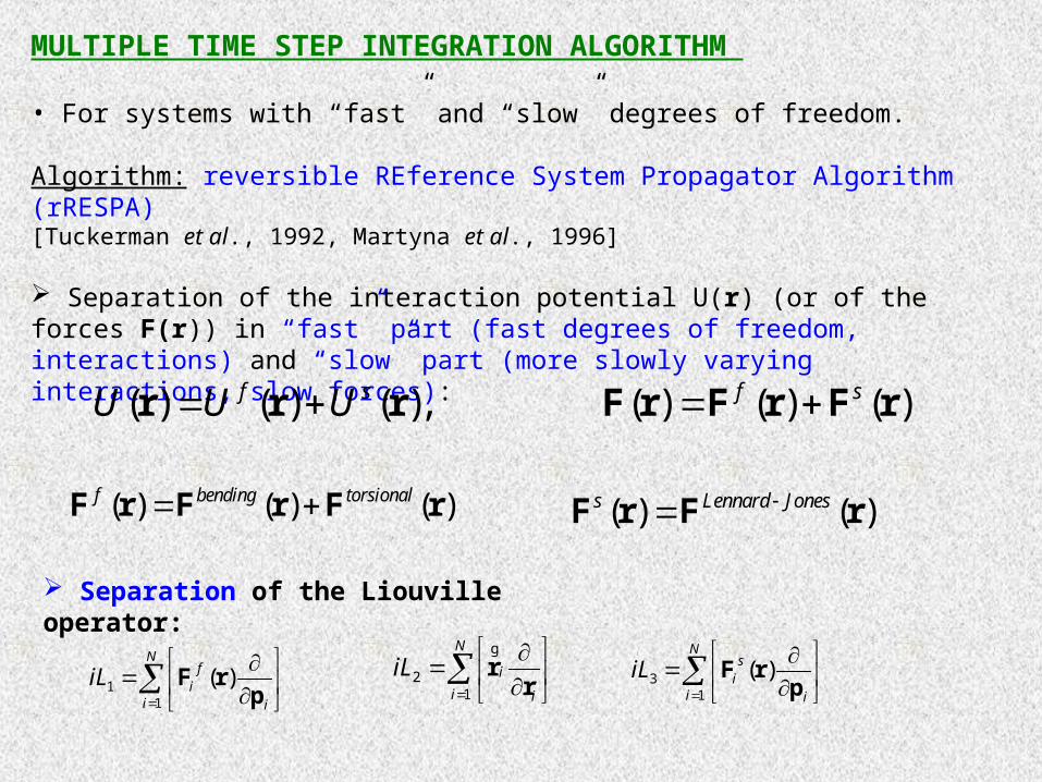
MULTIPLE TIME STEP INTEGRATION ALGORITHM

• For systems with “fast” and “slow” degrees of freedom.

Algorithm: reversible REference System Propagator Algorithm (rRESPA) [Tuckerman et al., 1992, Martyna et al., 1996] Separation of the interaction potential U(r) (or of the forces F(r)) in “fast” part (fast degrees of freedom, interactions) and “slow” part (more slowly varying interactions, slow forces):

( ) ( ) ( ), ( ) ( ) ( )f s f sU U U r r r F r F r F r

( ) ( ) ( )f bending torsional F r F r F r ( ) ( )s Lennard JonesF r F r

Separation of the Liouville operator:

11

( )N

fi

i i

iL F rp

2

1

N

i

i i

iL

r

r

g

31

( )N

si

i i

iL F rp

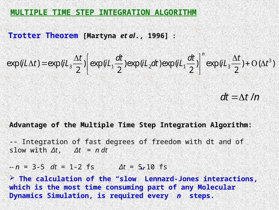
Trotter Theorem [Martyna et al., 1996] :

33 1 2 1 3exp( ) exp( ) exp( )exp( )exp( ) exp( ) ( )

2 2 2 2

nt dt dt t

iL t iL iL iL dt iL iL t

Advantage of the Multiple Time Step Integration Algorithm:

-- Integration of fast degrees of freedom with dt and of slow with Δt, Δt = n dt

/dt t n

So the calculation of the “slow” Lennard-Jones interactions, which is the most time consuming part of any Molecular Dynamics Simulation, is required every n steps.


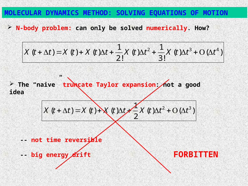
N-body problem: can only be solved numerically. How?

2 3 41 1( ) ( ) ( ) ( ) ( ) ( )

2! 3!X t t X t X t t X t t X t t t

The “naive” truncate Taylor expansion: not a good idea

2 31( ) ( ) ( ) ( ) ( )

2X t t X t X t t X t t t

-- not time reversible

-- big energy drift

MOLECULAR DYNAMICS METHOD: SOLVING EQUATIONS OF MOTION

FORBITTEN

2 4( ) 2 ( ) ( ) ( ) ( )X t t X t X t t X t t t

MOLECULAR DYNAMICS METHOD: SOLVING EQUATIONS OF MOTION

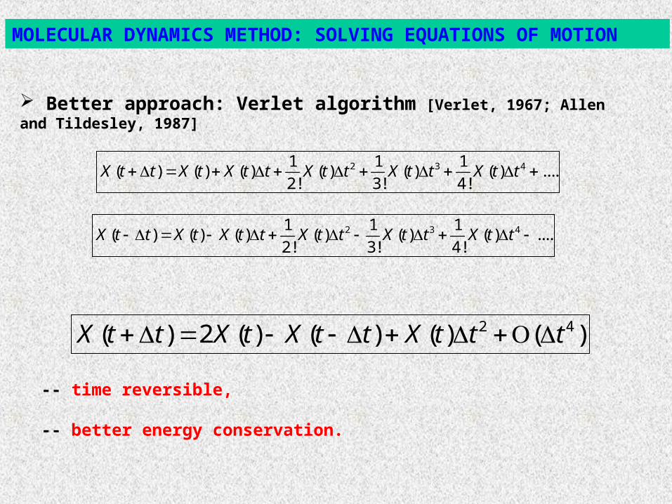
Better approach: Verlet algorithm [Verlet, 1967; Allen and Tildesley, 1987]

2 3 41 1 1( ) ( ) ( ) ( ) ( ) ( ) ....

2! 3! 4!X t t X t X t t X t t X t t X t t

-- time reversible,

-- better energy conservation.

2 3 41 1 1( ) ( ) ( ) ( ) ( ) ( ) ....

2! 3! 4!X t t X t X t t X t t X t t X t t

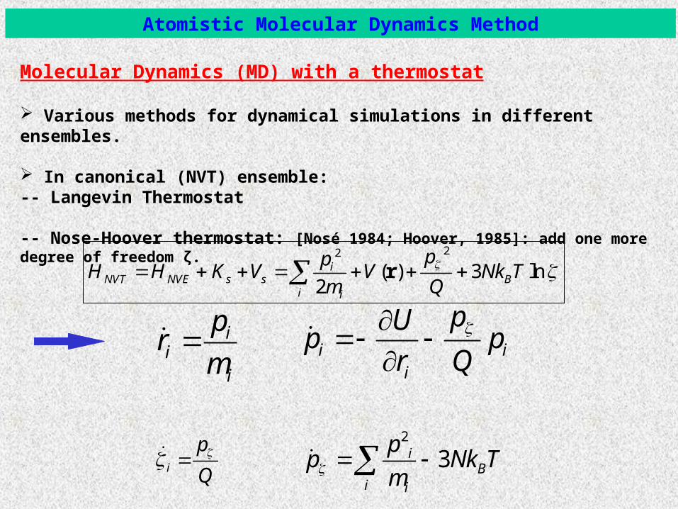
Molecular Dynamics (MD) with a thermostat

Various methods for dynamical simulations in different ensembles.

In canonical (NVT) ensemble:-- Langevin Thermostat

-- Nose-Hoover thermostat: [Nosé 1984; Hoover, 1985]: add one more degree of freedom ζ.

i

p

Q

2

3 iB

i i

pp Nk T

m

ii

i

pr

m

i i

i

pUp p

r Q

22

( ) 3 ln2

iNVT NVE s s B

i i

ppH H K V V Nk T

m Q r


Molecular Dynamics (MD) [Alder and Wainwright, J. Chem. Phys., 27, 1208 (1957)]

Classical mechanics: solve classical equations of motion in phase space (r, p).

In microcanonical (NVE) ensemble:

Liouville operator:

The evolution of system from time t=0 to time t is given by : ( ) exp (0)t iLt

1

,N

i ii i i

iL H

r Fr p

gK

ii

i

pr

m c

ii

Up F

r

2

( )2

iNVE

i i

pH K V V

m rHamiltonian (conserved quantity):


Trotter Theorem [Martyna et al., 1996] :

33 1 2 1 3exp( ) exp( ) exp( )exp( )exp( ) exp( ) ( )

2 2 2 2

nt dt dt t

iL t iL iL iL dt iL iL t

Advantage of the Multiple Time Step Integration Algorithm:

-- Integration of fast degrees of freedom with dt and of slow with Δt, Δt = n dt

-- n = 3-5 dt = 1-2 fs Δt = 5-10 fs

/dt t n

The calculation of the “slow” Lennard-Jones interactions, which is the most time consuming part of any Molecular Dynamics Simulation, is required every n steps.


Bulk Polyethylene

Atomistic MD Simulations: Applications

-- Various polymer lengths from C40, to C300

(M=4800) for times up to 100 ns.

-- T = 450 K > Tm

-- Equilibration: using a powerful MC algorithm (Theodorou et al, 1999)

United-atom (UA) description

TraPPE model (Siepmann et al, 1998)

Multiple Time Step (Martyna et al., 1996)

[Harmandaris et al. Macromolecules, 1998; 2000; 36, 1376, 2003]

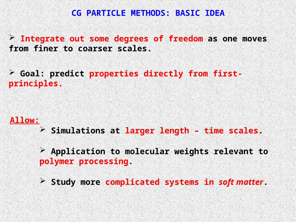
CG PARTICLE METHODS: BASIC IDEA

Integrate out some degrees of freedom as one moves from finer to coarser scales.

Allow: Simulations at larger length – time scales.

Application to molecular weights relevant to polymer processing.

Study more complicated systems in soft matter.

Goal: predict properties directly from first-principles.

MESOSCOPIC BOND STRETCHING POTENTIAL OF PS

Distribution function PCG(r,T)

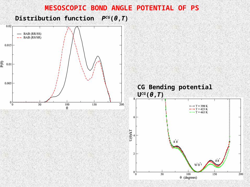
MESOSCOPIC BOND ANGLE POTENTIAL OF PS

Distribution function PCG(θ,T)

CG Bending potential UCG(θ,T)

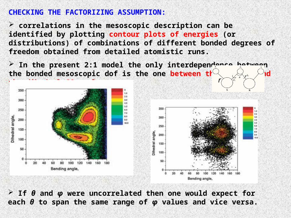
CHECKING THE FACTORIZING ASSUMPTION:

correlations in the mesoscopic description can be identified by plotting contour plots of energies (or distributions) of combinations of different bonded degrees of freedom obtained from detailed atomistic runs.

In the present 2:1 model the only interdependence between the bonded mesoscopic dof is the one between the bending and the dihedral CG angle.

If θ and φ were uncorrelated then one would expect for each θ to span the same range of φ values and vice versa.

r


Reversible work method

[McCoy and Curro, Macromolecules, 31, 9362 (1998)]

Obtained for each CG bead independently:

By calculating the reversible work (potential of mean force) U(r,T) between the centers of mass of two isolated molecules as a function of distance:

exp ,( , ) lnCG ATnb U rU r T

,

,AT ATij

i j

U r U r

Average < > over all degrees of freedom Γ that are integrated out (here orientational ) keeping the two center-of-masses fixed at distance r.

CG NONBONDED EFFECTIVE INTERACTION POTENTIAL

CG effective potential: Different type of CG particles.

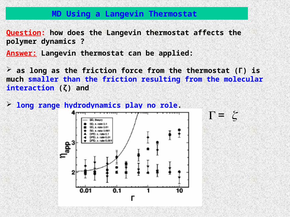
Question: how does the Langevin thermostat affects the polymer dynamics ?

MD Using a Langevin Thermostat

Answer: Langevin thermostat can be applied:

as long as the friction force from the thermostat (Γ) is much smaller than the friction resulting from the molecular interaction (ζ) and

long range hydrodynamics play no role.

Γ

=

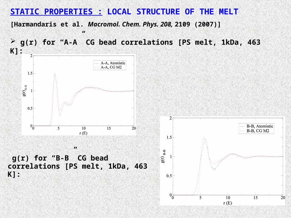
STATIC PROPERTIES : LOCAL STRUCTURE OF THE MELT

[Harmandaris et al. Macromol. Chem. Phys. 208, 2109 (2007)]

g(r) for “A-A” CG bead correlations [PS melt, 1kDa, 463 K]:

g(r) for “B-B” CG bead correlations [PS melt, 1kDa, 463 K]:

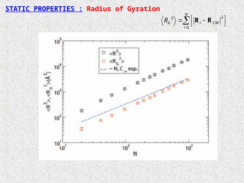
STATIC PROPERTIES : Radius of Gyration22

1

N

G i CMi

R

R R

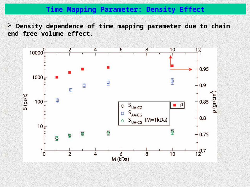
Time Mapping Parameter: Density Effect

Density dependence of time mapping parameter due to chain end free volume effect.

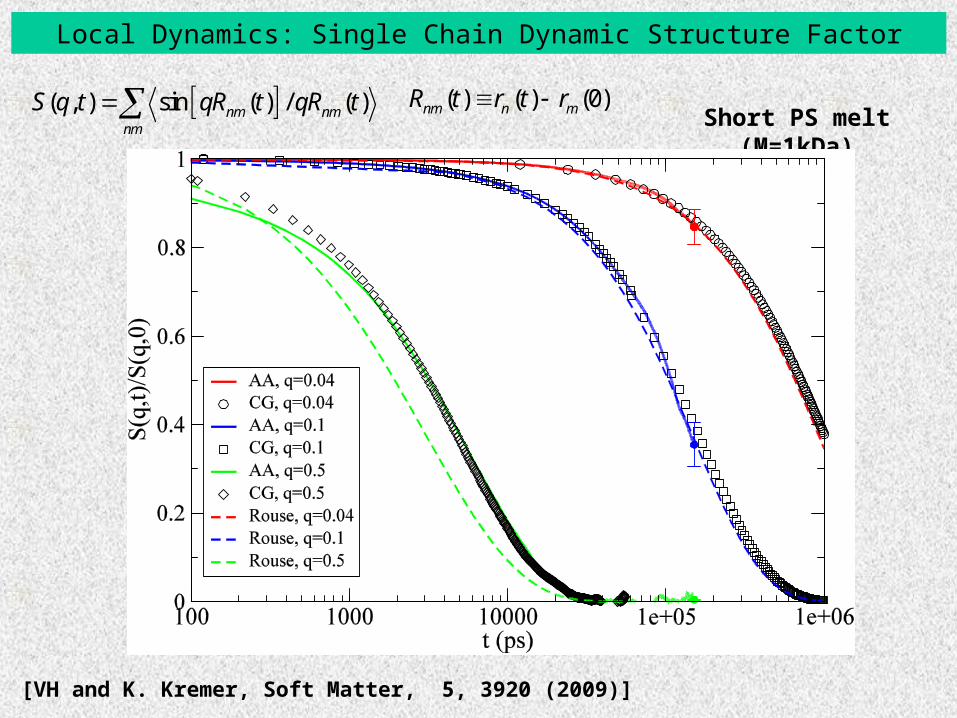
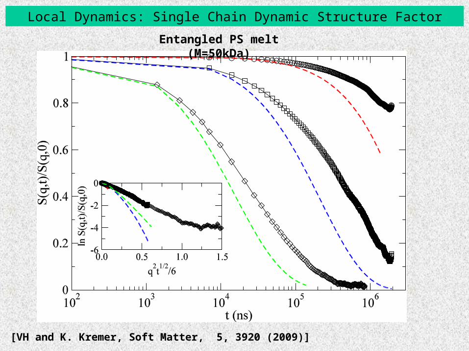
Local Dynamics: Single Chain Dynamic Structure Factor

Short PS melt (M=1kDa)

[VH and K. Kremer, Soft Matter, 5, 3920 (2009)]

( , ) sin ( ) / ( )nm nmnm

S q t qR t qR t ( ) ( ) (0)nm n mR t r t r

Local Dynamics: Single Chain Dynamic Structure Factor

[VH and K. Kremer, Soft Matter, 5, 3920 (2009)]

Entangled PS melt (M=50kDa)

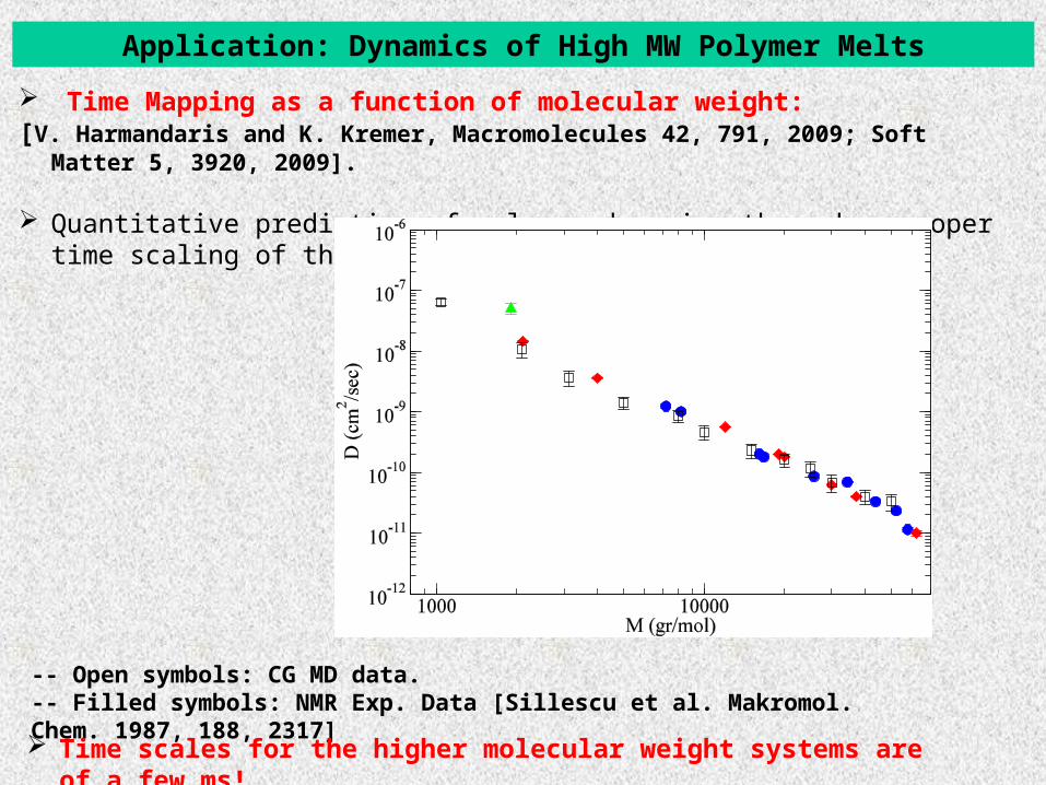
Application: Dynamics of High MW Polymer Melts

Time Mapping as a function of molecular weight: [V. Harmandaris and K. Kremer, Macromolecules 42, 791, 2009; Soft Matter 5, 3920, 2009].

Quantitative prediction of polymer dynamics through a proper time scaling of the CG data.

-- Open symbols: CG MD data.-- Filled symbols: NMR Exp. Data [Sillescu et al. Makromol. Chem. 1987, 188, 2317]

Time scales for the higher molecular weight systems are of a few ms!

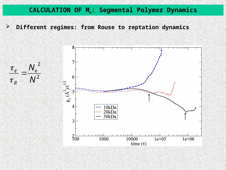
Different regimes: from Rouse to reptation dynamics

2

2

N

Ne

R

e

CALCULATION OF Me: Segmental Polymer Dynamics

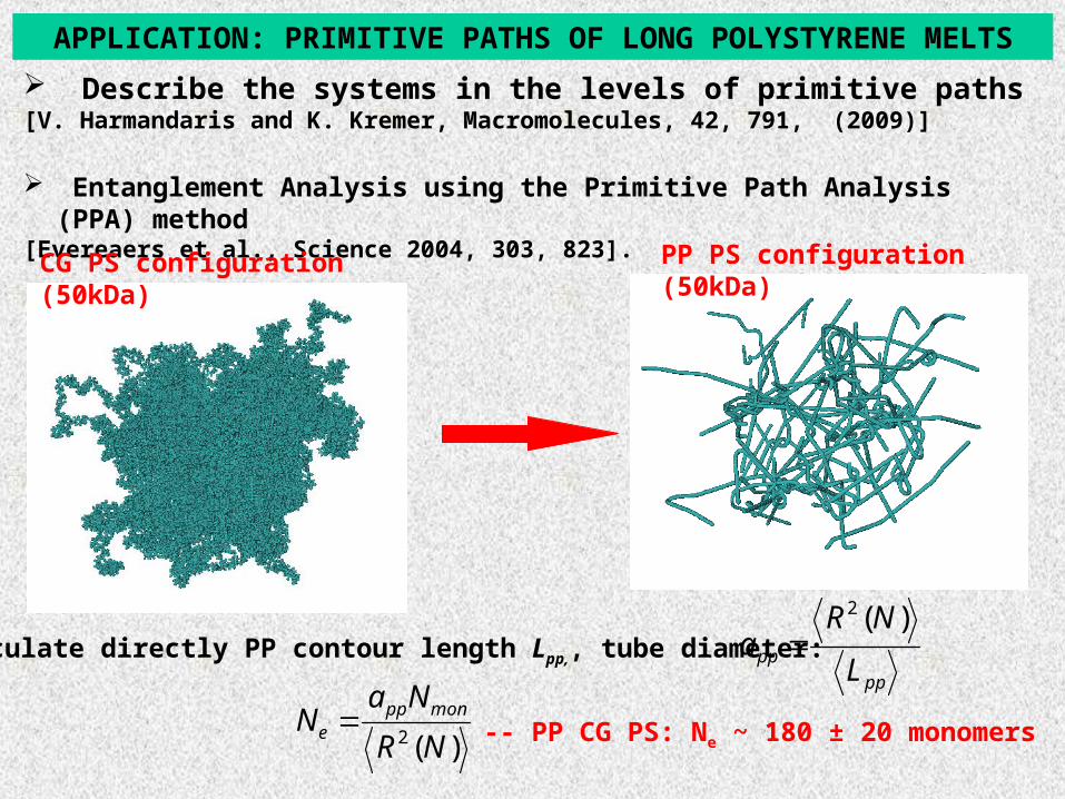
APPLICATION: PRIMITIVE PATHS OF LONG POLYSTYRENE MELTS

Describe the systems in the levels of primitive paths[V. Harmandaris and K. Kremer, Macromolecules, 42, 791, (2009)]

Entanglement Analysis using the Primitive Path Analysis (PPA) method[Evereaers et al., Science 2004, 303, 823].

CG PS configuration (50kDa) PP PS configuration (50kDa)

pp

ppL

NRa

)(2

Calculate directly PP contour length Lpp,, tube diameter:

)(2 NR

NaN monpp

e -- PP CG PS: Ne ~ 180 ± 20 monomers

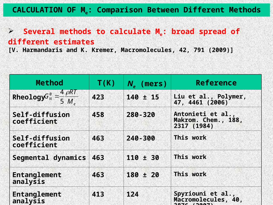
CALCULATION OF Me: Comparison Between Different Methods

Several methods to calculate Me: broad spread of different estimates [V. Harmandaris and K. Kremer, Macromolecules, 42, 791 (2009)]

Method T(K) Ne (mers) Reference

Rheology 423 140 ± 15 Liu et al., Polymer, 47, 4461 (2006)

Self-diffusion coefficient 458 280-320 Antonieti et al., Makrom. Chem., 188, 2317 (1984)

Self-diffusion coefficient 463 240-300 This work

Segmental dynamics 463 110 ± 30 This work

Entanglement analysis 463 180 ± 20 This work

Entanglement analysis 413 124 Spyriouni et al., Macromolecules, 40, 3876 (2007)

eN M

RTG

5

40


Study segmental dynamics as a function of temperature and pressure. [V. Harmandaris, G. Floudas and K. Kremer, Macromolecules 44, 393 (2011)]


2 ( ) exp KWWtt

tP A

Fit with KWW functions:


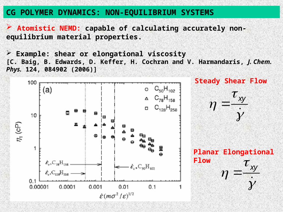
Atomistic NEMD: capable of calculating accurately non-equilibrium material properties.

Example: shear or elongational viscosity[C. Baig, B. Edwards, D. Keffer, H. Cochran and V. Harmandaris, J. Chem. Phys. 124, 084902 (2006)]

CG POLYMER DYNAMICS: NON-EQUILIBRIUM SYSTEMS

xy

xy

Steady Shear Flow

Planar Elongational Flow

Atomistic NEMD: capable of calculating accurately non-equilibrium material properties. Example: shear or elongational viscosity [C. Baig, et al., J. Chem. Phys. 124, 084902 (2006)]

CG Polymer Simulations: Non-Equilibrium Systems

CG NEMD - Remember: CG interaction potentials are calculated as potential of mean force (they include entropy)

Important question: How well polymer systems under non-equilibrium (flowing) conditions can be described by CG models developed at equilibrium?

( , ) ln , , ( , , )CG CG CG CG CGBU T k T P T x x x r

In principle UCG(x,T) should be obtained at each state point, at each flow field.

Very difficult due to high computational demands. Desirable to use (existing) equilibrium CG potentials.

Short atactic PS melts (M=2kDa, 20 monomers) are studied by both atomistic and CG NEMD simulations.

CG NEMD Simulations – Application: Polystyrene under Shear Flow

NVT Ensemble. Nose – Hoover thermostat (T=463K).

Multiple time step method.

Periodic boundary conditions.

Use of existing equilibrium CG polystyrene (PS) model.

Direct comparison between atomistic and CG NEMD simulations for various flow fields.

Strength of flow (Weissenberg number, Wi = 0.3 - 200) Wi

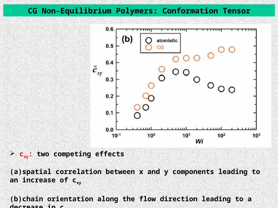
CG Non-Equilibrium Polymers: Conformation Tensor

cxy: two competing effects

(a)spatial correlation between x and y components leading to an increase of cxy

(b)chain orientation along the flow direction leading to a decrease in cxy.

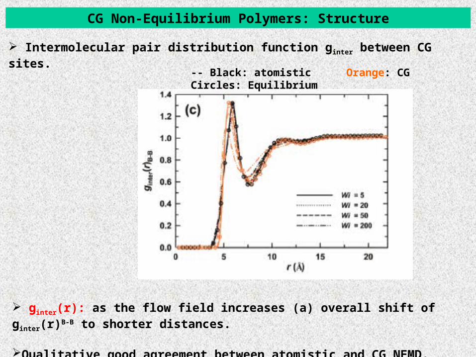
CG Non-Equilibrium Polymers: Structure

Intermolecular pair distribution function ginter between CG sites.

-- Black: atomistic Orange: CG Circles: Equilibrium

ginter(r): as the flow field increases (a) overall shift of ginter(r)B-B to shorter distances.

Qualitative good agreement between atomistic and CG NEMD.

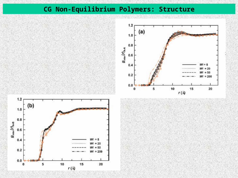
CG Non-Equilibrium Polymers: Structure

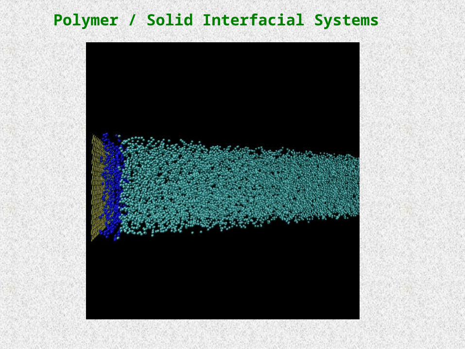
Polymer / Solid Interfacial Systems

COARSE-GRAINED PARTICLE MODELING

Dynamical speed up:

-- Acceleration due to the decrease in the number of freedoms (16 atoms or 8 “united atoms” are replaced by 2 beads).

-- Time step in the mesoscopic dynamic simulations, dtCG = 20-30 fs.

-- Speed up due to faster dynamics: S ~ 10

-- Overall speed up of the mesoscopic dynamic simulations, compared with the atomistic, is ~ 3 orders of magnitude.

Good results: homogeneous systems (melts), high temperatures (systems where many-body terms are not important).

Problematic: low temperatures, mixtures (systems where many-body terms become important)

VAGELIS HARMANDARIS ACMAC Workshop: Coarse-graining of many-body systems: analysis, computations and...

Documents

Transcript of VAGELIS HARMANDARIS ACMAC Workshop: Coarse-graining of many-body systems: analysis, computations and...