CHEMICAL ENGINEERING LABORATORY

CHEG 4137

Osmotic Separations: Reverse and Forward Osmosis

Objective:

The objective of this experiment is to evaluate the performance of various membranes when used for

reverse osmosis (RO) and forward osmosis (FO) applications. The impact of operating conditions such

as solute concentration, pressure, flow rate, and temperature on separation efficacy will be examined.

This experiment combines several aspects of fluid mechanics and mass transport, illustrating how flow

conditions impact mass transport through the membrane. Ultimately, students will be able to determine

which process the provided membranes are best-suited for, as well as optimal operating conditions for

each.

Major Topics Covered: Mass transfer, fluid mechanics, boundary layer theory, colligative properties

Theory:

Osmotic desalination using membranes is a way to remove salts and other solutes from water sources,

ultimately generating fresh, potable water. The benefit of membrane desalination over alternate

desalination methods, such as evaporation, is membrane separations do not cause a phase change

which, as a result, consumes less energy. An established membrane desalination technique is RO,

where a pressure gradient is applied in excess of the feed solution's osmotic pressure to force water

through the membrane while salts are retained. An emerging desalination technique is FO, were the

membrane divides the feed solution and a concentrated draw solution. Water from the feed solution

flows into the draw naturally by osmosis. In an FO system designed for desalination, the draw solution

is either designed to be ingested or easily recoverable. In this experiment, however, the draw solute

will be sodium chloride. For a more technical overview of theory for this experiment, consult the

supplemental osmosis theory document. Additionally, the works of Baker (1), Mulder (2), Sablani (3),

Cath (4), McCutcheon & Elimelech (5,6), and Geankoplis (7) may be useful in the preparation of your

report.

Safety Precautions:

1. Be sure that reservoir tanks are full and all appropriate lines are connected before turning on any

of the pumps.

2. When handling membranes, always wear protective gloves to prevent fouling of the membranes.

3. Systems operate under pressure so safety glasses should be worn at all times.

Available Variables:

For RO: Membrane type (NF90, NF270, BW30, SW30), feed solute concentration, pressure, feed flow

rate, temperature

For FO: Draw solute concentration, feed flow rate, draw flow rate, pressure, temperature

Note: You will not have time to test all possible variables. Be sure to consider which parameters you

think would be most important to permeability and selectivity.

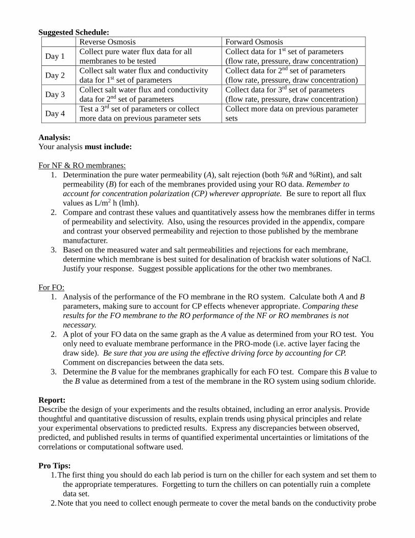
Suggested Schedule:

Reverse Osmosis Forward Osmosis

Day 1 Collect pure water flux data for all

membranes to be tested

Collect data for 1st set of parameters

(flow rate, pressure, draw concentration)

Day 2 Collect salt water flux and conductivity

data for 1st set of parameters

Collect data for 2nd set of parameters

(flow rate, pressure, draw concentration)

Day 3 Collect salt water flux and conductivity

data for 2nd set of parameters

Collect data for 3rd set of parameters

(flow rate, pressure, draw concentration)

Day 4 Test a 3rd set of parameters or collect

more data on previous parameter sets

Collect more data on previous parameter

sets

Analysis:

Your analysis must include:

For NF & RO membranes:

1. Determination the pure water permeability (A), salt rejection (both %R and %Rint), and salt

permeability (B) for each of the membranes provided using your RO data. Remember to

account for concentration polarization (CP) wherever appropriate. Be sure to report all flux

values as L/m2 h (lmh).

2. Compare and contrast these values and quantitatively assess how the membranes differ in terms

of permeability and selectivity. Also, using the resources provided in the appendix, compare

and contrast your observed permeability and rejection to those published by the membrane

manufacturer.

3. Based on the measured water and salt permeabilities and rejections for each membrane,

determine which membrane is best suited for desalination of brackish water solutions of NaCl.

Justify your response. Suggest possible applications for the other two membranes.

For FO:

1. Analysis of the performance of the FO membrane in the RO system. Calculate both A and B

parameters, making sure to account for CP effects whenever appropriate. Comparing these

results for the FO membrane to the RO performance of the NF or RO membranes is not

necessary.

2. A plot of your FO data on the same graph as the A value as determined from your RO test. You

only need to evaluate membrane performance in the PRO-mode (i.e. active layer facing the

draw side). Be sure that you are using the effective driving force by accounting for CP.

Comment on discrepancies between the data sets.

3. Determine the B value for the membranes graphically for each FO test. Compare this B value to

the B value as determined from a test of the membrane in the RO system using sodium chloride.

Report:

Describe the design of your experiments and the results obtained, including an error analysis. Provide

thoughtful and quantitative discussion of results, explain trends using physical principles and relate

your experimental observations to predicted results. Express any discrepancies between observed,

predicted, and published results in terms of quantified experimental uncertainties or limitations of the

correlations or computational software used.

Pro Tips:

1. The first thing you should do each lab period is turn on the chiller for each system and set them to

the appropriate temperatures. Forgetting to turn the chillers on can potentially ruin a complete

data set.

2. Note that you need to collect enough permeate to cover the metal bands on the conductivity probe

for saline feed tests. You shouldn’t have to collect more than 15-20 mL of permeate per sample

cylinder under any circumstances. Budget your time appropriately.

3. The scale for the FO system is sensitive to slight breezes, so to speed up the equilibration process,

it is recommended to leave the system alone for a period of time, and do not touch the tank or

scale. When adding salt, add the stock solution, take appropriate readings, and walk away.

4. Always make sure the computer is collecting data!

5. If you notice water isn’t flowing in the FO system, turn off the pumps and make sure all quick-

disconnect fittings are completely connected. Sometimes these connections stick.

6. Keep in mind that the maximum pressure for the FO systems is 10 psi.

7. The FO review paper by Cath et al (4) is an excellent resource; it contains many equations that

are relevant to both experiments.

References:

1. Baker, Richard W., Membrane Technology and Applications, 2nd Edition, John Wiley & Sons,

Ltd. (2004), Chapters 4 & 5

2. Mulder, Marcel, Basic Principles of Membrane Technology, 2nd Edition, Kluwer Academic

Publishers (1996), Chapters 6 & 7

3. Sablani et al, “Concentration polarization in ultrafiltration and reverse osmosis: a critical

review,” Desalination 141 (2001) 269-89

4. Cath, Childress, and Elimelech. “Review: Forward osmosis: Principles, applications, and recent

developments.” Journal of Membrane Science 281 (2006) 70-87

5. McCutcheon, Jeffrey R. and Elimelech, Menachem. “Modeling Water Flux in Forward

Osmosis: Implications for Improved Membrane Design.” AIChE Journal 53 (2007). 1736-44

6. McCutcheon, Jeffrey R. and Elimelech, Menachem. “Influence of concentrative and dilutive

internal concentration polarization on flux behavior in forward osmosis.” Journal of Membrane

Science 284 (2006) 237-47.

7. Geankoplis, Christie J., Transport Processes and Separation Process Principles, 4th Edition,

Prentice-Hall (2003), Chapters 6 & 13

Supplemental Resources from Dow Water & Process Solutions:

Dow Water & Process Solutions Information for NF270:

http://www.dow.com/PublishedLiterature/dh_0074/0901b803800749e1.pdf?filepath=liquidseps/pdfs/noreg/609-00519.pdf&fromPage=GetDoc

Dow Water & Process Solutions Information for NF90:

http://www.dowwaterandprocess.com/products/membranes/nf90_400.htm

Dow Water & Process Solutions NaCl Rejections for NF Membranes:

NF270: %R = 50%

NF90: %R = 90-96%

Source: http://dow-answer.custhelp.com/app/answers/detail/a_id/4925/~/filmtec-membranes---nanofiltration---mwco

Dow Water & Process Solutions Information for BW30:

http://www.dow.com/PublishedLiterature/dh_0182/0901b80380182f51.pdf?filepath=liquidseps/pdfs/noreg/609-00091.pdf&fromPage=GetDoc

CHEMICAL ENGINEERING LABORATORY

CHEG 4137W/4139W

Osmotic Separations: Reverse Osmosis (RO) Supplemental Theory

The goal of RO desalination is to extract significant quantities of potable water from saltwater using a

selective membrane. The membrane is designed to allow water to pass through while retaining solutes.

As the saltwater is pressurized, pure water passes through the membrane into the permeate stream. The

salt and water that does not permeate the membrane leaves the system as retentate. A basic RO system

block diagram is shown in Figure 1 below:

Figure 1: RO system diagram, the dashed line represents the membrane

The general equation for water flux in a reverse osmosis process is:

In the above equation, Jw is water flux, A is the hydraulic permeability constant of the membrane, P is

the transmembrane hydraulic pressure gradient, and eff is the effective transmembrane osmotic

pressure gradient. Note that flux has units of volume of permeate per area of membrane per time

(either gallons/ft2 day or liter/m2 h). Hydraulic permeance has units of flux per pressure (either gfd/psi

or lmh/bar). The hydraulic permeability constant is a property of the membrane itself and is a function

of membrane thickness, porosity, pore tortuosity, and temperature.

Osmotic pressure is a colligative property that indicates how much solute is dissolved in water. It can

be calculated using the van’t Hoff equation, shown in equation 2. Note that this form of the van’t Hoff

equation is used to determine the osmotic pressure of ideal solutions.

In the van’t Hoff equation, note that C is the molar concentration of solute ions in solution, R is the gas

constant, and T is the temperature. The van’t Hoff equation cannot be used to directly solve for , the

difference between the osmotic pressures of the feed and permeate. Under what conditions could

be equal to the osmotic pressure of the bulk feed solution?

It is important to know that effective osmotic pressure gradient (eff) refers to the osmotic pressure

gradient on both sides of the membrane interface. Note that this gradient is NOT equivalent to the

observed, or bulk, concentration gradient (obs), which is the difference in osmotic pressure between

the bulk feed and permeate. This distinction must be made as a result of concentration polarization

(CP) effects. As water flows through the membrane, salt is brought to the membrane surface via

convection. Unable to pass the membrane, the solute collects at the membrane’s surface, forming a

boundary layer, as shown in Figure 2. The rate of salt diffusion out of the boundary layer, dictated by

the mass transfer coefficient k, is dependent upon fluid flow characteristics within the membrane

channel.

Bulk feed Permeate

Retentate

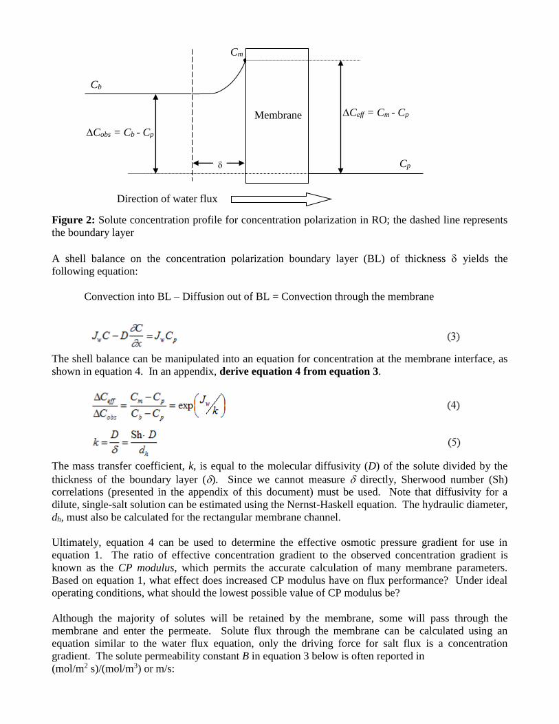
Figure 2: Solute concentration profile for concentration polarization in RO; the dashed line represents

the boundary layer

A shell balance on the concentration polarization boundary layer (BL) of thickness yields the

following equation:

Convection into BL – Diffusion out of BL = Convection through the membrane

The shell balance can be manipulated into an equation for concentration at the membrane interface, as

shown in equation 4. In an appendix, derive equation 4 from equation 3.

The mass transfer coefficient, k, is equal to the molecular diffusivity (D) of the solute divided by the

thickness of the boundary layer (). Since we cannot measure directly, Sherwood number (Sh)

correlations (presented in the appendix of this document) must be used. Note that diffusivity for a

dilute, single-salt solution can be estimated using the Nernst-Haskell equation. The hydraulic diameter,

dh, must also be calculated for the rectangular membrane channel.

Ultimately, equation 4 can be used to determine the effective osmotic pressure gradient for use in

equation 1. The ratio of effective concentration gradient to the observed concentration gradient is

known as the CP modulus, which permits the accurate calculation of many membrane parameters.

Based on equation 1, what effect does increased CP modulus have on flux performance? Under ideal

operating conditions, what should the lowest possible value of CP modulus be?

Although the majority of solutes will be retained by the membrane, some will pass through the

membrane and enter the permeate. Solute flux through the membrane can be calculated using an

equation similar to the water flux equation, only the driving force for salt flux is a concentration

gradient. The solute permeability constant B in equation 3 below is often reported in

(mol/m2 s)/(mol/m3) or m/s:

Cb

Cp

Cm

Membrane Ceff = Cm - Cp

Cobs = Cb - Cp

Direction of water flux

In order to easily quantify the separation effectiveness, salt rejection must be calculated. Rejection is

the difference between the solute concentrations in the feed and permeate streams divided by the solute

concentration of the feed. If concentration cannot be measured directly, solution conductivity () may

be used for this calculation. The observed salt rejection calculation is as follows:

Intrinsic rejection (Rint), the rejection of the membrane based on the concentrations at the membrane

interface, can also be calculated as follows:

Since CP increases the effective solute concentration at the membrane interface, what effect does this

have on , water flux, and overall system performance? If it is assumed that Cp << Cb, how can the

CP modulus equation be simplified? Is this assumption valid given your experimental conditions?

Why or why not?

Knowing Rint allows for a direct calculation of B as follows:

Sherwood Number Correlations (from Mulder):

Source: Mulder, Marcel. Basic Principles of Membrane Technology, 2nd Edition. Kluwer Academic Publishers (1996)

CHEMICAL ENGINEERING LABORATORY

CHEG 4137W/4139W

Osmotic Separations: Forward Osmosis (FO) Supplemental Theory

Osmotic Pressure as a Driving Force:

The goal of FO is to extract water from a feed solution using a concentrated draw solution. The driving

force behind this separation is a difference in osmotic pressure (). Water will flow through the

membrane to the area of greater osmotic pressure in an attempt to decrease the osmotic pressure

gradient, as shown in the diagram below:

Figure 1: Basic FO membrane diagram, the dashed line represents the membrane

Osmotic pressure is a colligative property that is directly proportional to solute concentration. It can be

calculated using the van’t Hoff equation, shown below for an ideal solution:

In the van’t Hoff equation, C is the molar concentration of solute ions in solution, R is the gas constant,

and T is the temperature.

The general equation for water flux in a forward osmosis process is:

In the above equation, Jw is water flux, A is the hydraulic permeability constant of the membrane, D is

the osmotic pressure of the draw solution, and F is the osmotic pressure of the feed. The subscript m

indicates that these osmotic pressure values are evaluated at the membrane interface. Note that flux has

units of volume of permeate per area of membrane per time (i.e. gallons/ft2 day). Hydraulic

permeability is reported as a flux per pressure (i.e. gfd/psi). If the feed is pure water, how will equation

2 simplify? How would you modify this equation to account for a transmembrane pressure gradient?

Concentration Polarization (CP):

As with any membrane process, the performance of a forward osmosis system can be affected by a

phenomenon called concentration polarization (CP). CP occurs as water flows from the feed to the

draw. Unlike reverse osmosis, CP can occur on both sides of the membrane. A diagram of external

concentration polarization phenomena occurring in FO is shown in Figure 2:

Concentrated Draw

Solution

(D)

Dilute Feed Solution

(F)

Direction of water flux

Figure 2: External concentration profile for a membrane operating in FO mode; the dashed line

represents the boundary layers with thickness , C refers to solute concentration

On the feed side, as water permeates the membrane, solutes flow towards the membrane by convection.

As the membrane is designed to reject these solutes, a solute boundary layer forms at the membrane’s

surface. This boundary layer increases the concentration of solute at the membrane surface, resulting

in an osmotic pressure that’s higher at the membrane interface than in the bulk feed solution. This

phenomenon is called concentrative external concentration polarization (ECP). In this experiment,

however, the feed solution is pure water. Under these circumstances, would you expect external CP on

the feed side to have a significant impact on membrane performance?

On the draw side of the membrane, the water flux creates lowers the solute concentration at the

membrane interface. As a result, the osmotic pressure at the membrane surface is lower than the

osmotic pressure in the bulk draw solution. This phenomenon is called dilutive ECP. What is the

overall impact that ECP has on the driving force of the FO process? What effect does this phenomenon

have on water flux and overall membrane performance?

Performing a shell balance on the draw-side boundary layer yields the following:

Convection through membrane = Convection out of BL – Diffusion into BL

Integrating this differential equation with respect to the boundary conditions yields an equation for CP

modulus, which is the ratio of Ceff to Cobs:

Concentrated Draw

Solution Dilute Feed

Solution

D F

Direction of water flux

CD,b

CF

CD,m

Membrane

CF,m

Cobs = CD,b – CF,b Ceff = CD,m – CF,m

This equation assumes the only CP effects are external and on the draw side (i.e. feed side CP is

negligible). The mass transfer coefficient k can be determined using the Sherwood number correlations

presented in the appendix. Diffusivity (D) can be calculated for dilute, single-salt solutions using the

Nernst-Haskell equation. Be sure to calculate the hydraulic diameter, dh, for the rectangular membrane

channel.

A more complex facet of CP is dilutive internal concentration polarization (ICP). ICP is predominantly

observed when the membrane is run in FO mode, where the active layer is placed against the draw

solution (when the active layer is placed against the feed solution, it is called PRO mode). As water

flows through the membrane’s support layer, salt concentration gradually decreases. As a result, the

effective concentration gradient around the active layer becomes much less than the observed

concentration gradient, as shown on the diagram on the next page.

While determining all the parameters required to calculate the degree of ICP in FO mode is beyond the

scope of this experiment, we are still able to quantify the degree of ICP. Using equations 1, 2, and 4,

flux can be predicted using your experimental conditions (concentration, fluid velocity, etc.).

Figure 3: Internal concentration profile for a membrane in FO mode, where C is concentration

What is the actual driving force for forward osmosis when accounting for CP effects? Keeping your

experimental conditions (i.e. feed and draw solution solute concentrations) in mind, how can this

equation be simplified? How can equations 1 and 4 be combined to predict flux values for a membrane

with known hydraulic permeance and given feed and draw solution concentrations? Using the shell

balance presented in the documentation for the RO experiment, present a derivation of equation 4 as an

appendix in your report.

Salt Flux:

Although the membrane is designed to reject salts, some of salt will pass from the draw solution into

the feed. In order to quantify the separation effectiveness, we must calculate salt flux. Salt flux is

governed by the equation below:

In equation 6, B is the salt permeability constant of the membrane and Cd and Cf are the solute

concentration of the draw and feed, respectively. B should be calculated graphically and compared to

the calculation of B based on RO tests. Similar to water flux, salt flux (Js) has units of mass flow rate

of salt through the membrane per unit area of membrane (i.e. kg/ft2 day).

Sherwood Number Correlations (from Mulder):

Source: Mulder, Marcel. Basic Principles of Membrane Technology, 2nd Edition. Kluwer Academic Publishers (1996)

CHEMICAL ENGINEERING LABORATORY

CHEG 4137W

Reverse Osmosis Operation Procedure

Preliminary Preparation:

1. Calibrate the conductivity probe using 8-10 solutions of different concentrations. Make sure

both metal bands on the probe are covered.

a. Tip: Start with a small concentration, such as 0.02M, and increase the concentration until

you reach 2.0M or 3.0M

2. Make sure the water level in the chiller is between the minimum and maximum lines. If you

need to add water, do so using deionized water.

3. Turn on the chiller; the chiller should be set to somewhere between 19.3 and 19.8oC.

4. Fill each cell with a very small amount of deionized water prior to adding the membranes.

5. While wearing gloves, load a membrane into each cell, active layer down. For RO, the shiny

side of the membrane should be facing down.

6. Place the top half of the cell on top of the membrane. Place the washers and nuts on the

designated bolts. Tighten each cell with a wrench or ratchet.

7. Place the permeate tubes into a waste beaker or flask.

8. Fill the feed tank with 9 L distilled water.

9. Making sure all appropriate valves are open/closed and all fittings are connected, turn on the

pump. If using the system with the variable frequency drive, the frequency should be set to 15.

The bypass valves on both systems have an arrow on the handle showing the flow path.

When the flow is bypassing the air purge line, the valve is considered “closed.” See

below for valve “closed” positions for both systems. If you need to change to position of

the valve, do so when the pump is off – otherwise water will jet out of the air purge line.

System A System B

10. Once all the air bubbles are purged from the system, set the pressure by slowly and carefully

adjusting the needle valve and pressure regulator. Also set the desired flowrate. Note that

closing the silver pressure regulator will increase pressure and crossflow rate while closing the

green needle valve will increase pressure while lowering crossflow rate.

11. Allow the membranes to equilibrate at pressure for approximately 10-15 minutes, until all air is

flushed from the permeate lines (water is exiting all the cell outlet tubes).

Starting a Test:

1. Weigh the three graduated cylinders. It’s a good idea to weigh them when dry and when slightly

wetted.

2. Record permeate flow rate for 3-5 different pressures for pure water.

a. The first pressure is already set (from step 10 above). Start collecting the outlet water

from the permeate lines in the graduated cylinders and start the timer.

b. After 5-10 minutes, record the collection time, weigh the graduated cylinders, then dump

the water back into the feed tank. Repeat this step to obtain a second data point.

i. Note: Calculations will be simpler if you keep the collection time constant

throughout your trials

c. Change the pressure to the next setting, allow the system to equilibrate for 5-10 minutes,

then repeat the data collection procedure detailed above.

d. Repeat step 2c for all desired pressure settings.

3. Based on your prelab calculation, create a 1L solution with enough NaCl to create a 2000ppm

saline feed. Add to the feed tank and allow approximately 10 minutes for the feed to mix.

4. Record the permeate flow rate and permeate conductivity at various crossflow rates and/or

pressures. Take these readings every 10-15 minutes for 30 minutes. Don’t forget to record the

conductivity of the feed tank as well.

a. Make sure both metal bands on the conductivity probe are covered when taking

conductivity readings

Shut-Down Procedure: Must be completed before having your exit checklist form signed by the TA.

1. Turn off the pump and chiller, then drain the feed tank using the drain valve. Make sure that no

air enters the pump.

2. Refill the feed tank with about 10L of tap water. Detach the return lines and place them in a

bucket. Flush the system twice with tap water (about 10L each time), then with about 10L of

distilled water.

When flushing the system, do not let any air into the pumps. This can damage the

pump and shorten the pump life. Pay close attention and turn off the pump before air can

reach the pump.

3. Open the bypass valve. Valves in the “open” position can be see below.

System A System B

4. Using a compressed air line, air purge the system using the quick disconnect fittings placed near

the bypass valve. Use a low amount of air pressure (less than 200 kPa) and never fully connect

the fittings – this would damage the pressure gauges.

5. Open each cell and remove the membranes, which can be disposed of once they have been

examined for defects. Leave the cells open.

CHEMICAL ENGINEERING LABORATORY

CHEG 4137W/4139W

Forward Osmosis Operation Procedure

Note: Maximum pressure for the FO systems is 10psi.

Preliminary Preparation:

1. Prepare a 1L volumetric flask of stock solution of 5M NaCl. Do not shake this flask! Place a

stirbar in the flask and stir using a stirplate until all NaCl is in solution. While this is mixing,

move on to the next step. When the mixing is complete, remove the stir bar and dilute to

volume.

2. Place a stir bar in the blue feed tank. Fill the feed and draw tanks with 2L DI water. Make sure

the tanks are disconnected from the lines when filling with water.

3. Make sure the water level in the chiller is between the minimum and maximum lines. If you

need to add water, do so using deionized water.

4. Turn on the chiller.

5. While wearing gloves, load a membrane into the cell, making a note of the membrane’s

orientation. Make sure the membrane fully covers the inner O-ring but does not touch the outer

O-ring.

6. Place the top half of the cell on top of the membrane. Place the washers and nuts on the

designated bolts. Tighten the cell with a wrench or ratchet.

7. Connect all quick-disconnect fittings.

8. Start the data acquisition software.

System A:

Note: Do not open another excel workbook while the program is running.

Double click on Pinnacle USB and press Ctrl+L.

Select “Open Log File” and name your file. You can create a folder for your group’s

data in the “CHEG Lab” folder.

Upon clicking OK, Excel will open. Click “Start Data Log” to begin data acquisition.

Feel free to change the time interval.

System B:

Note: The macro is finicky. Do not open another excel workbook while the macro is running.

Open a new Excel workbook.

Under the Developer tab, select “Visual Basic.”

Under the “File” menu, select “Import.”

The file is located in Documents and is named “Module1.bas” – import this file.

Return to the Excel workbook and select “Macros” under the Developer tab.

Select the macro titled “FO_Test” and click “Run.”

The workbook should look like this:

To being data collection, change the Time Interval to a value greater than 0. This value is

measured in seconds and determines how often the macro collects data from the scale.

9. Turn on the pumps, setting the flow to approximately 1 L/min. You may opt to run at a higher

flow at first to flush air bubbles out, but be sure to keep transmembrane pressure at zero.

10. Allow the membrane to equilibrate until the minute-to-minute change in draw solution mass is

less than 0.05 g/min. This should take roughly 15-20 minutes.

11. While waiting for the system to equilibrate, calibrate the conductivity probe using 8-10

solutions of different concentrations. Make sure both metal bands on the probe are covered.

a. Tip: Start with a small concentration, such as 0.02M, and increase the concentration until

you reach 2.0M or 3.0M

Performing a Test:

1. Calculate the appropriate amount of 5M NaCl stock solution needed to obtain the desired draw

concentration, then add this to the draw tank to start the test. Record feed solution conductivity,

temperature, and appropriate flow rates.

2. Allow the data acquisition software to record the mass of the draw solution every 60 seconds

until the system has reached equilibration; this will take approximately 20-30 minutes.

3. After the system has reached equilibration, add the amount of stock solution needed for the next

draw concentration. Simultaneously record feed conductivity and temperature.

4. Periodically make sure the data acquisition software is running – if the computer goes to sleep,

you may lose data.

Shut-Down Procedure: Must be completed before having your exit checklist form signed by the TA.

1. Turn off the pumps.

2. Click “Stop Data Log” in Pinnacle (System A) or change the Time Interval to “0” in the excel

sheet (System B). Make sure you save your data and quit the program.

3. Drain each tank in the sink and refill each with about 2L tap water. Reconnect all fittings and

run the pumps for approximately five minutes to flush the system. Flush each tank twice with

tap water (2L each tank each time), then once with 2L of DI water each.

4. Using a compressed air line, air purge the system using the quick disconnect fittings placed after

each pump. Use a low amount of air pressure (less than 200kPa) and never fully connect the

fittings – this would damage the pressure gauges.

5. Open the cell and remove the membranes, which can be disposed of once they have been

examined for defects. Leave the cell open.