71

CHAPTER 3

MATERIALS AND METHODS

The thesis work has been carried out to develop the indigenous 3D Radiation Field

Analyzer , dosimetric and commissioning of FFF beam and clinical use of FFF beam

for complex targets. All the measurement of FFF beam was done with Varian True

Beam machine available at Health Care Global Enterprise, Ahmadabad.

3.1 Radiation filed Analyzer

In order to develop an indigenous RFA preliminarily the work was categorically

divided into three parts such as,

i) Development of water phantom, telescopic column lifting assembly, three

stepper motors integration with water phantom and development of hand

control for manual movements of stepper motors.

ii) Development of software for beam data acquisition using Microsoft Visual

basic 6 software and development of data analyzing software for obtaining

data as per International/National protocols.

iii) Integration of dual channel electrometer, the stepper motor Linear Motion

(LM) guide assembly and the data acquisition software.

3.1.1 Design of water phantom

Water phantom was made with 15 mm thick acrylic material with 800 x 750 x 570

mm size. UV pasting were used to ensure „no water leakage‟ when filled with water.

The larger size of the phantom was to accommodate the LM guide and stepper motor

assembly. The Figure 3.1 shows the CAD diagram of indigenous RFA in all three

views.

72

Figure 3.1 : CAD diagram of indigenous RFA.

a) Complete View b) Sagital View

c) Coronal View

73

3.1.2 Telescopic Lifting Mechanism

The Lift table is a separate water phantom carriage with electrically operated lifting

mechanism for the positioning of the water phantom. The carriage has two fixed and

two steerable rollers with breakers. The cabinet has one compartment and two drawers

for storing accessories and is furthermore equipped with a leveling frame for fine

adjustment in vertical and horizontal directions.

The lifting mechanism is capable of lifting 700 kgs with stroke of 40cm and the speed

set at 5 mm/sec on max load (can be increased up to 15mm) intended to avoid any jerk

and wobbling of water phantom during movement. The lifting assembly is provided

with a 2 button pendent for operation. The load bearing frame is fitted with four heavy

duty caster wheels with locking options. The phantom lifting platform has 4 degrees

of adjustment to account for the leveling of floor or phantom. The overall height was

kept at 1450mm for the lifting mechanism.

3.1.3 LM guide and Ball Screw

Linear motion systems are unique motion systems in which linear motion is supported

by rolling contact elements. These linear motion systems can best be described as a

motion system which uses the rotational motion principle of a deep grooved ball

bearing. The combined LM and lead screw is known as linear actuator. A lead screw

also known as a power screw is a screw designed to translate turning motion into

linear motion.

An electric motor was mechanically connected to rotate the lead screw. The lead

screw has a continuous helical thread machined on its circumference running along the

length (similar to the thread on a bolt). Threaded onto the lead screw is a lead nut or

ball nut with corresponding helical threads. The nut is prevented from rotating with

the lead screw (typically the nut interlocks with a non-rotating part of the actuator

body). Therefore, when the lead screw is rotated, the nut will be driven along the

74

threads. The direction of motion of the nut will depend on the direction of rotation of

the lead screw. By connecting linkages to the nut, the motion can be converted to

usable linear displacement. The design and developed in this study used stepper

motor and high precision stainless steel moving mechanism.

3.1.4 Stepper Motor

A stepper motor is a brushless DC electric motor that divides a full rotation into a

number of equal steps. The motor's position can then be commanded to move and hold

at one of these steps without any feedback sensor (an open-loop controller).

Conventional AC and DC motors operate on continuously applied input voltage and

most often produce a continuous (steady state) rotary motion. Most commercial type

motors are single phase, equipped with two lead wires, or three lead wires, the third

lead normally used as a grounding lead. Current flows from one lead wire into the

motor and returns through the other lead wire. Unlike these motors, a Stepper motor

(also called a stepping motor) will not produce continuous motion from a continuous

input voltage. It will stay at a particular position as long as the power is “on”. An

electrical phase change is necessary to make a stepper motor move in a particular

direction. This means that no single phase step motor can exist. A typical three phase

stepper motor has four lead wires. Three of them represent the three phase coils,

normally colored with brown, red, and in orange. The fourth lead is a common lead for

current return, commonly colored with black or in white. Turning one phase “on” will

hold the rotor in one position (called a detent position). Turning “off” this phase and

turning on the second phase will move the rotor to rest at another detent position. This

“on and off” current flow is called a pulse. One pulse into the motor causes the rotor to

increment (move) one precise angle. This movement is repeated with each input pulse.

When properly applied and controlled, the number of output steps is always equal to

the number of input pulses. The widespread acceptance of the digital approach for

overall control of machine and process functions has generated a high demand for

75

mechanical motion devises capable of delivering a discrete incremental motion of

known accuracy. The replacement of less dependable (susceptible to wear) mechanical

devices, such as clutches and breaks, with stepper motors, provides considerably

greater reliability and consistency.

A stepper motor needs to be part of a stepper motor system. A Stepper motor system is

made up of 3 basic elements often combined with some form of user interface

(computer, dumb terminal, PLC) , This interface system is used to send commands to

the system. The Controller/Indexer is a microprocessor that generates the step pulses

and direction signals for the driver. The controller typically performs many other

sophisticated command functions as well. Most controllers have onboard memory so

they can store thousands of commands. In this study, three stepper motor for X, Y and

Z positioning were used which had the speed of 40 mm/s and accuracy of ± 0.5 mm.

All three stepper motor are controlled by the control console system through driver

card. The motors can also be controlled locally by the Human Machine Interface

(HMI) pendent which communicates through the same driver card.

3.1.5 Three - Axis controller driver Card

The Galil motion controller is designed for operation with many different types of

motors. The signal conditioning circuits used to control different types of motors have

been built into the controller and allow the user to interface with different motors

easily.When the controller is powered on with the stepper motor plugged into the

linear stage on, the stepper motor will no longer be able to move. This means that the

stepper motor is energized and is ready to begin motion. Using e DMC smart terminal

software, create a new program named stepper control. When using a stepper motor

there are specific parameters that need to be set to accurately control the motor. One

of the first parameters that should be set are type of motor been connected. Using the

command KSX 2 tells the controller that a stepper motor is being used. KSX 2 is the

command used to tell the controller what type of motor and 2 tells the controller it is a

76

stepper motor. once that the type of motor is selected, the acceleration, deceleration

and speed of the motor must be defined. To set the acceleration of the motor the

command AC defines the acceleration rate of the motor. The deceleration of the

motor is defined using the DC command and the speed of the motor is defined using

the SP command. All of the commands range in value from 1 to 100000 cycles per

second with 1 being the slowest speed and 100000 being the fastest.

Once these parameters are set the motor needs to be provide with the movement

instruction. To move the stepper motor the command PA is used which tells the

controller where to move. These values range from 0 to 2000000 with 0 not moving

the stepper motor at all and 2000000 which will move the motor to the end of the

stage. Once the motor is told where to move the motor starts its motion once the BG

command is entered. An example of the sample code for movement is shown below.

#MOVESTEP

MTX=2; 'Set the type of motor

SPX=11000; 'Set the speed of the motor

ACX=10000; 'Set the acceleration of the motor

DCX=10000000; 'Set the deceleration of the motor

PAX=10000

EN 'End the program

3.1.6 Human Machine Interface (HMI)

Human machine interface(HMI) is the part of the machine that handles the Human-

machine interaction. membrane switches, rubber keypads and touch screens are

examples of Human Machine Interface which we can operate by seeing and touching.

It provides a graphics-based visualization of an industrial control and monitoring

system. An HMI typically resides in an office-based Windows computer that

communicates with a specialized computer in the plant such as a programmable

77

automation controller (PAC), programmable logic controller (PLC) or distributed

control system (DCS).

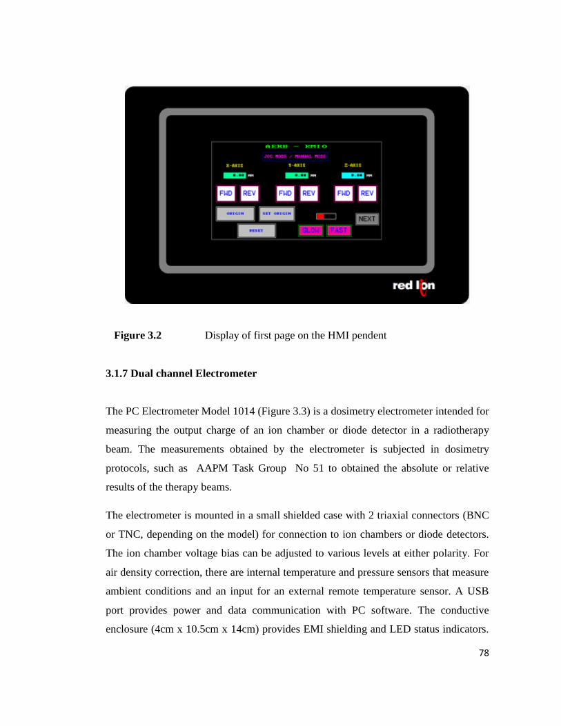
A local pendent to control to adjust the X, Y and Z movements in the LM assembly

was developed using HMI. The pendent was designed with two page operation to

provide all the required functions. The HMI pendent was developed with touch screen

technology. The first page has the following buttons of operation (Figure 3.2 )

a) X, Y,Z forward/reverse switch

b) Virtual home

c) Define home

d) Machine home

e) Speed selection (Fast/Slow)and

f) Next Button

The Next button provided in the first page will take the operator to the second

page, which has the following operations.

a) X, Y, Z value entry for desired movements

b) Start and

c) Speed selection

78

Figure 3.2 Display of first page on the HMI pendent

3.1.7 Dual channel Electrometer

The PC Electrometer Model 1014 (Figure 3.3) is a dosimetry electrometer intended for

measuring the output charge of an ion chamber or diode detector in a radiotherapy

beam. The measurements obtained by the electrometer is subjected in dosimetry

protocols, such as AAPM Task Group No 51 to obtained the absolute or relative

results of the therapy beams.

The electrometer is mounted in a small shielded case with 2 triaxial connectors (BNC

or TNC, depending on the model) for connection to ion chambers or diode detectors.

The ion chamber voltage bias can be adjusted to various levels at either polarity. For

air density correction, there are internal temperature and pressure sensors that measure

ambient conditions and an input for an external remote temperature sensor. A USB

port provides power and data communication with PC software. The conductive

enclosure (4cm x 10.5cm x 14cm) provides EMI shielding and LED status indicators.

79

The calibrated Dual channel electrometer has dose rate of 0.001pA – 500.0 pA, 1 fA

resolution (Low Range) and 0.001nA – 500.0 nA, 1 pA resolution (High Range). In

charge mode the ranges are 0.001pC – 999.9 μC, 1 fC resolution (Low Range) and

0.001 nC – 999.9 μC, 1 pC resolution (High Range). Repeatability of the electrometer

is ± 0.1% (IEC 60731 requirement: ± 0.5%)(10). Three preset bias voltages of 0, ±

150, ± 300 volts can be used.The bias voltages can also be set independently to fulfill

our custom needs. The electrometer was procured along with the calibration

certificate.

Figure 3.3: PC Electrometer

3.1.8 Ionization chamber

The ionization chambers of 0.125cc (Standard Imaging Inc. USA) is used for both

reference and field measurements. The cylindrical chamber has 36mm rigid stem with

inner diameter of 5.5mm. The chamber has an aluminum electrode with 1mm diameter

and 5mm long. The chambers are energy independent from 30KeV to 50 MeV range.

For both the chambers the calibration certificates were obtained.

Figure 3.4 A18 Model cylindrical chamber (0.125cc)

80

The Model A18 chamber features exceptional spatial resolution for relative dosimetry

scanning, and is capable of measuring small field sizes. Calibration caps constructed

with the same material as the major elements of the chamber were available to

provide more than adequate build-up for Cobalt-60 radiation. Its waterproof

construction makes it ideal for use in water phantoms. The chamber vents through a

flexible tube that surrounds the triaxial cable, ensuring the collecting volume is in

pressure equilibrium with the surroundings.

Features and Benefits

Proven guard design yields stable, precise measurements and minimizes

settling time by creating uniform field lines

Shell, collector, and guard are all made of durable, long lasting Shonka

conductive plastic

Use of homogeneous material throughout the chamber minimizes perturbation

of the beam due to the presence of the chamber and optimizes measurements

Axially symmetric design of the chamber provides an uniform, isotropic

response

Inherent waterproof construction eliminates need for additional protective

coverings

Non-removable one piece stem for easy, precise positioning

A matching 2.0 mm thick Cobalt-60 build-up cap of C552 Shonka air-

equivalent plastic is provided for air calibrations and measurements

Ionization collection efficiency is always 99.9% or better

Collecting volume is 0.125 cc

3.1.9 Beam Analysis Software

The software for radiation beam analyzer was developed in the Microsoft Visual basic

6.0 platform. With Visual Basic 6, user will find it easier to capture and analyze

81

information to help them make effective decisions. Visual Basic 6 enables user of

every size to rapidly create more secure, manageable, and reliable applications. The

dosimetry common object module (COM) was developed to support the RFA.

The dosimetry COM object was developed support the following threads and objects:

Each COM object is associated with one and only one apartment. This is

decided at the time the object is created at runtime. After this initial setup, the

object remains in that apartment throughout its lifetime.

A COM thread (i.e., a thread in which COM objects are created or COM

method calls are made) is also associated with an apartment. Like COM

objects, the apartment with which a thread is associated is also decided at

initialization time. Each COM thread also remains in its designated apartment

until it terminates.

Threads and objects which belong to the same apartment are said to follow the

same thread access rules. Method calls which are made inside the same

apartment are performed directly without any assistance from COM.

Threads and objects from different apartments are said to play by different

thread access rules. Method calls made across apartments are achieved via

marshalling. This requires the use of proxies and stubs.

The Graph com object should designed to handle the demanding requirements

of server side usage. It multi-threaded design handles multiple concurrent

requests quickly and efficiently

Linear and Log scales with full font support

Up to 8000 profiles in one chart

Up to 1,000,000 samples per profile

Y scale stacking

X and Y value for each data point

Built-in zoom, scrollbars and pan

Crosshairs and coordinates display

82

Boolean profiles and scales

Stair Mode profiles

Pass data point-by-point

Pass entire arrays directly for best performance with a lot of data

Read/edit/set any value in the data array

Auto and manual scale modes for all scales

Manually set each scale's major tick interval

Set toolbar tool tips for multiple languages Date Time formatting down to ms

Units support for each scale

Grid for each scale

Pan individual scales when no scrollbars

Legend with scrolling when needed

Coordinates available programmatically

Null data points for breaks in a profile

Global number and date time formatting

Full documentation help and sample code

Save chart image to bitmap or metafile

Copy chart image to clipboard

Export chart data to tab delimited text file

Use your own toolbar

Extensive property pages

Flickerless display, even when resizing

Error log file for detailed debugging

Different software modules required by the RFA system that were developed are

i. Beam Scanning module

ii. Beam data analysis

1. Import other vendor file module

83

2. Protocol library module

3. Result display module

3.1.9.1 Beam Scanning Module

Beam scanning module controls the stepper motor, LM guide mechanism and the dual

channel electrometer. Before collecting the radiation beam data, the electrometer can

be reset for residual charges by choosing the „zeroing‟ option. The option to set the

bias voltage is also provided in the window (0,-300,+300 etc,).

Before the commencement of actual data collection, it is mandatory to feed the type

of radiation unit, energy, field size, SSD, wedge angle, gantry angle, collimator angle

etc. to the developed RFA software. The screen shot indicating these options are

shown in Figure 3.5.

In the same window, the provision for direct selection of PDD, In plane profile, Cross

plane profile, Diagonal (Left-Right) profile and Diagonal (Right-Left) profiles can be

obtained for multiple depths and multiple field sizes. All the profiles are displayed in

the same live window. Additionally an option is provided to select the PDD scan

direction (Top-Bottom or Bottom-Top).

84

Figure 3.5 A typical beam scanning module screen

Before obtaining the actual profile, the detector will get aligned to the preset home

position (0, 0, 0 coordinates) and then the collection of data occurs for profile. The

system is programmed in such a way that on completion of each scan the system will

automatically normalize the maximum reading to 100%.

While collecting the in-plane or cross-plane profiles the detector will move to collect

beam data by calculating the scan starting point from the fed field size and the

penumbral margin information. The software is developed in such a way that the

detector checks for the shortest distance from its current position to start the scan.

Beam scan software has the ability to set the speed of chamber, step size and chamber

measurement time and also the developed software provides the option to control or

85

move the chamber in X, Y, and Z direction. The screen shot of the developed

software with all the above said information is provided in Figure 3.6.

Figure 3.6 A typical beam scanning option module screen

3.1.9.2 Beam data analysis

3.1.9.2.1 Import other vendor file module

The scan data of other commercially available RFA can be imported for analyzing in

the developed software. When the scan files of other vendors are imported the data is

programmed to convert those files into file extension format of the developed

software which is .rba (Radiation Beam Analyser) attached to each file. This module

provides option to check the scanned data of other vendors with developed software

and vice-versa.

3.1.9.2.2 Protocol library

Figure 3.7: A typical option menu screen

86

The variable option available to view the profile. Continuous beam option will

provide the value of X and Y in the graph continuously and discrete option will show

only the measured X and Y value. The screen shot of the developed menu option

provided is shown in figure 3.7. Various standard protocol libraries were made

available in the developed software for the convenience of the users such as AERB,

IAEA, DIN, TG 45 etc. A typical screen indicating the selection options is presented

in figure 3.8.

Figure 3.8 A typical protocol selection screen

Analysis parameters for profiles

Beam Flatenss :

The beam flatness is assessed by finding the maximum Dmax and minimum Dmin dose

point values on the beam profile within the central 80% of the beam width and then

using the following relationship:

87

a) Percentage dose difference to IEC 60976 (2007)

(Eq.3.1)

b) Percentage Dose Ratio ( PTW RFA User manual )

(Eq.3.2)

c) Filed Ratio (PTW RFA User manual )

(Eq.3.3)

d) Maximum Variation (PTW RFA User manual )

(Eq.3.4)

Standard linac specifications generally require that flatness to be less than 3% when

measured in a water phantom at a depth of 10 cm with an SSD of 100 cm.

Beam Symmetry :

The beam symmetry is usually determined at Dmax, which represents the most

sensitive depth for assessment of this beam uniformity parameter. A typical symmetry

specification is that any two dose points on a beam profile, equidistant from the central

axis point, are within 2% of each other (Kutcher et.al., 1994 ). Alternately, areas under

the Dmax beam profile on each side (left and right) of the central axis extending to the

88

50% dose level (normalized to 100% at the central axis point) were also determined as

symmetry. Some of the definitions of symmetry are

a) Maximum Dose Ratio to IEC60976 ( 2007)

(Eq.3.5)

D(x) is the dose at point x; x and -x are points within the flattened region, symmetrical

to the central axis. Symmetry is defined as being the maximum ratio within the

flattened region, multiplied with 100.

b) Area Ratio (PTW RFA User manual )

(Eq.3.6)

Where,

a = area to the left of the central axis

b = area to the right of the central axis

The areas are delimited by the central axis and the 50% field limit.

c) Maximum variation (PTW RFA User manual )

(Eq.3.7)

D(x) is the dose at point x; x and -x are points within the flattened region, symmetrical

to the central axis.

Field Size at SID (PTW RFA User manual )

The field size at isocenter determined by

89

(Eq.3.8)

Where ,

SID = Source Isocenter Distance in cm

F = Field Size for 50% dose in cm

SSD = Source Surface Distance in cm

D = Profile depth in cm

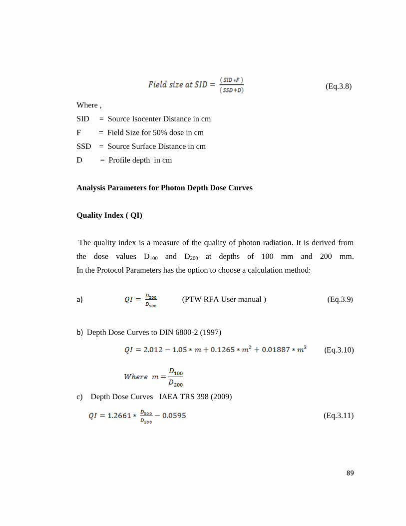
Analysis Parameters for Photon Depth Dose Curves

Quality Index ( QI)

The quality index is a measure of the quality of photon radiation. It is derived from

the dose values D100 and D200 at depths of 100 mm and 200 mm.

In the Protocol Parameters has the option to choose a calculation method:

a) (PTW RFA User manual ) (Eq.3.9)

b) Depth Dose Curves to DIN 6800-2 (1997)

(Eq.3.10)

c) Depth Dose Curves IAEA TRS 398 (2009)

(Eq.3.11)

90

Analysis parameters for electron depth dose curves :

R100 - Depth of the maximum dose

Practical range (Rp ) :

Depth at the intersection of X-ray background line and best fit line on the steep

sloping section of the curve.

Depth of the 50% dose ( R50 ) :

In the Protocol Parameters dialog has the option to choose a calculation method:

R50 = I50 ( Eq.3.12)

Rq : position of the intersection of the tangent at the inflection point of the curve

and the best fit line on the steep sloping section of the curve .

Percentage dose at the surface (Ds) :

IEC 60976 defines the surface dose as the dose at a depth of 0.5 mm.

X-Ray Bckground

X-ray background as a percentage of the maximum dose

In the protocol parameters dialog has option to choose a calculation method for x-ray

backround :

a) X-ray background is the dose of the intersection point of

calculation of Rp

b) X-ray background is the dose of the last measured point

Most probable energy at the phantom surface (Ep0 ) :

In the Protocol Parameters dialog you can choose a calculation method:

Dosimetry protocol to DIN 6800-2 (1997)

E0(mean) < 5: Ep,0 = 2.08 * Rp + 0.176 (Eq.3.13 )

E0(mean) ≥ 5: Ep,0 = 1.947 * Rp + 0.481 (Eq.3.14)

Mean energy at the phantom surface E0(mean) :

The protocol parameters dialog has the option to choose a calculation method for

obtaining E0(Mean) ,

91

a) Dosimetry protocol to DIN 6800-2(1997)

for ion dose:

E0(mean) = 0.348 + 2.2 * R50 + 0.017 * R50² (Eq.3.15)

for energy dose:

E0(mean) = 0.310 + 2.25 * R50 + 0.006 * R50² (Eq.3.16)

b) IPEMB dosimetry protocol

for ion dose:

E0(mean) = 0.818 + 1.935 * R50 + 0.040 * R50² (Eq.3.17)

for energy dose:

E0(mean) = 0.656 + 2.059 * R50 + 0.022 * R50² (Eq.3.18)

c) All other dosimetry protocols

E0(mean) = 2.33 * R50 (Eq.3.19)

Where , E0(mean) in MeV

R50 in cm

Figure 3.9 Graphical representation of parameters.

The figure 3.9 shows that the graphical representation of all electron parameter.

92

3.1.9.2.3 Result display module

The result obtained by the developed software will be displayed as per the parameters

selected by the uses. In single screen, the option of opening multiple profiles or

PDD‟s, Stretching/Skewing of windows were also made available in the developed

software. The displayed results may be converted in to ASCII or any other file format

as required by the any commercial available TPS. A typical 6 MV photon PDD for

10 x 10 cm2 field size obtained at 100 SSD with the display of results is shown in

Figure 3.10.

93

Figure 3.10 Result display screen along with the measured depth dose profile for

6MV photon beam for 10 x 10 cm2

.

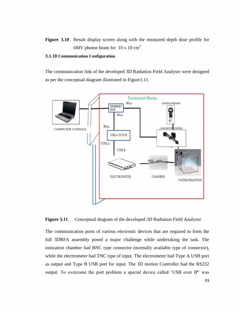
3.1.10 Communication Configuration

The communication link of the developed 3D Radiation Field Analyser were designed

as per the conceptual diagram illustrated in Figure3.11.

Figure 3.11 Conceptual diagram of the developed 3D Radiation Field Analyzer

The communication ports of various electronic devices that are required to form the

full 3DRFA assembly posed a major challenge while undertaking the task. The

ionization chamber had BNC type connector (normally available type of connector),

while the electrometer had TNC type of input. The electrometer had Type A USB port

as output and Type B USB port for input. The 3D motion Controller had the RS232

output. To overcome the port problem a special device called „USB over IP‟ was

COMPUTER CONSOLE

BNC cable

94

introduced in the electronics which will convert the electrometer output to RS232

output. This RS 232 output and the output from the 3D motion controller are

connected to an Ethernet Hub, through which the control console system

communicates with both the electrometer and motion controller uninterruptedly.

The completed RFA system indigenously developed for the study purpose is show in

Figure 3.12.

Figure 3.12 The developed 3D Radiation Field Analyzer.

95

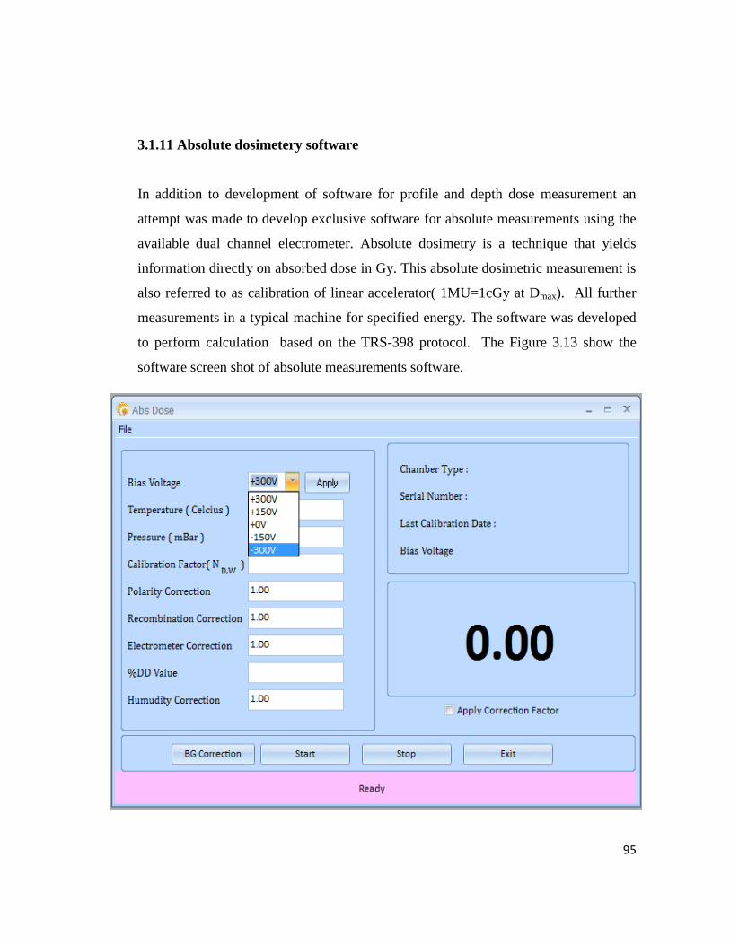
3.1.11 Absolute dosimetery software

In addition to development of software for profile and depth dose measurement an

attempt was made to develop exclusive software for absolute measurements using the

available dual channel electrometer. Absolute dosimetry is a technique that yields

information directly on absorbed dose in Gy. This absolute dosimetric measurement is

also referred to as calibration of linear accelerator( 1MU=1cGy at Dmax). All further

measurements in a typical machine for specified energy. The software was developed

to perform calculation based on the TRS-398 protocol. The Figure 3.13 show the

software screen shot of absolute measurements software.

96

Figure 3.13 Screen shows the absolute dosimetery software.

3.1.12 Premeasurement checks

The premeasruement checks were performed on the developed RFA system as per the

Task Group 106 recommendations (Das et.al., 2008). The noise, signal to noise ratio,

leakage, effect of polarity, effect of sampling time, effect of dose rate, effect of step

size were measured as per TG 106 recommendation.

3.1.13 Validation of the 3DRFA

The premeasurement checks were performed on the developed RFA system as per TG

106 recommendations. The physical parameters of photon PDDs such as Dmax, D10,

D20 and Quality Index, and the electron PDDs such as R50, Rp, E0, Epo and X-ray

contamination values can be obtained instantaneously by using the developed RFA

system. Also the results for profile data such as field size, Central axis deviation,

Penumbra, flatness and symmetry calculated according to various protocols can be

obtained for both photon and electron beams. The result of PDDs for photon beams

were compared with BJR25 (Jorden et al., 1996) supplement values and the profile

data were compared with TG 40 (Kutcher et al., 1994 ) recommendation.

3.1.14 FFF beam analysis using developed software

The characteristic of FFF beams were analyzed using developed RFA as per AERB

protocol. The symmetry of the beam is measured as per the IEC60976 (2007) as

described in Section 3.1.9.2.2.1. The stability of the beam FFF beams, lateral distance

from central axis at 90%, 75% and 60% dose points on either side of the beam profile

were measured using the developed RFA. The profile scan was acquired for 20x20

cm2

FS, SCD 100 cm at 10 cm depth. To find the inflection point , the measured data

97

exported to Microsoft excel file format and determined the field size and penumbra

for FFF as described in Section 3.2.6.

3.2 Commissioning and QA of FFF beam

The commissioning of FFF beams has been carried out for the first time in country.

The irradiation facilities and instruments used to acquire the beam data presented in

chapters 4, 5, 6 are briefed in this chapter.

The following dosimetric equipments were used in this study.

1. FFF linear accelerator (True Beam, Varian inc)

2. Radiation Filed Analyzer (IBA and indigenous

3. Electrometer with ion chambers ( Unidos, PTW)

4. 2D Array detection (Octavius PTW)

A brief description of the above equipments is given below,

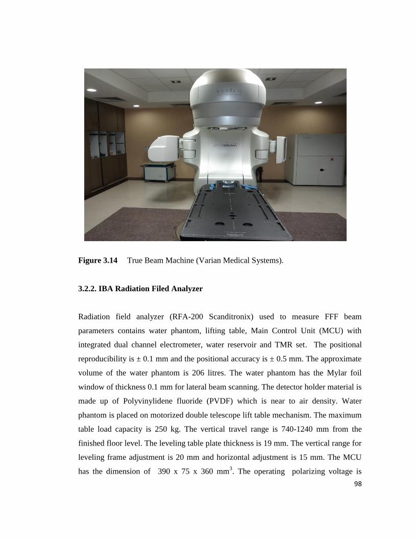
3.2.1 TRUE BEAM LINEAR ACCELERATOR

TrueBeam is the new model of medical linear accelerator from Varian Medical

Systems,USA, which was cleared by the FDA in December 2009. There are two

varieties available with this linac–TrueBeam and TrueBeam STx. The STx model is

intended for stereotactic use in addation to routinue usage of True Beam and has HD

MLC. A new feature for TrueBeam is the availability of the FFF mode. The photon

beams usually have a metal filter on their path to make photon fluence uniform (or

flat). With proliferation of accurate treatment planning algorithms and IMRT the

uniform fluence is not a concern, hence assumed to be advantageous with FFF mode.

When the filter is removed from the photon beam, the intensity increases by a factor of

2 for 6 MV photons and by a factor of 4 for 10 MV photons. A typical True beam

machine is shown in the Figure 3.14.

98

Figure 3.14 True Beam Machine (Varian Medical Systems).

3.2.2. IBA Radiation Filed Analyzer

Radiation field analyzer (RFA-200 Scanditronix) used to measure FFF beam

parameters contains water phantom, lifting table, Main Control Unit (MCU) with

integrated dual channel electrometer, water reservoir and TMR set. The positional

reproducibility is ± 0.1 mm and the positional accuracy is ± 0.5 mm. The approximate

volume of the water phantom is 206 litres. The water phantom has the Mylar foil

window of thickness 0.1 mm for lateral beam scanning. The detector holder material is

made up of Polyvinylidene fluoride (PVDF) which is near to air density. Water

phantom is placed on motorized double telescope lift table mechanism. The maximum

table load capacity is 250 kg. The vertical travel range is 740-1240 mm from the

finished floor level. The leveling table plate thickness is 19 mm. The vertical range for

leveling frame adjustment is 20 mm and horizontal adjustment is 15 mm. The MCU

has the dimension of 390 x 75 x 360 mm3. The operating polarizing voltage is

99

between -400 V to +400 V. The time constant is 40 ms and it contains 14 bit Analog

to Digital Converter (ADC) for optimized gain control. The maximum resolution is

0.1 pC with low range and 30 pC with high range. The leakage current is <0.5 pA with

low range and < 2 pA with high range. The MCU can communicate to computer

through RS232 connectivity.

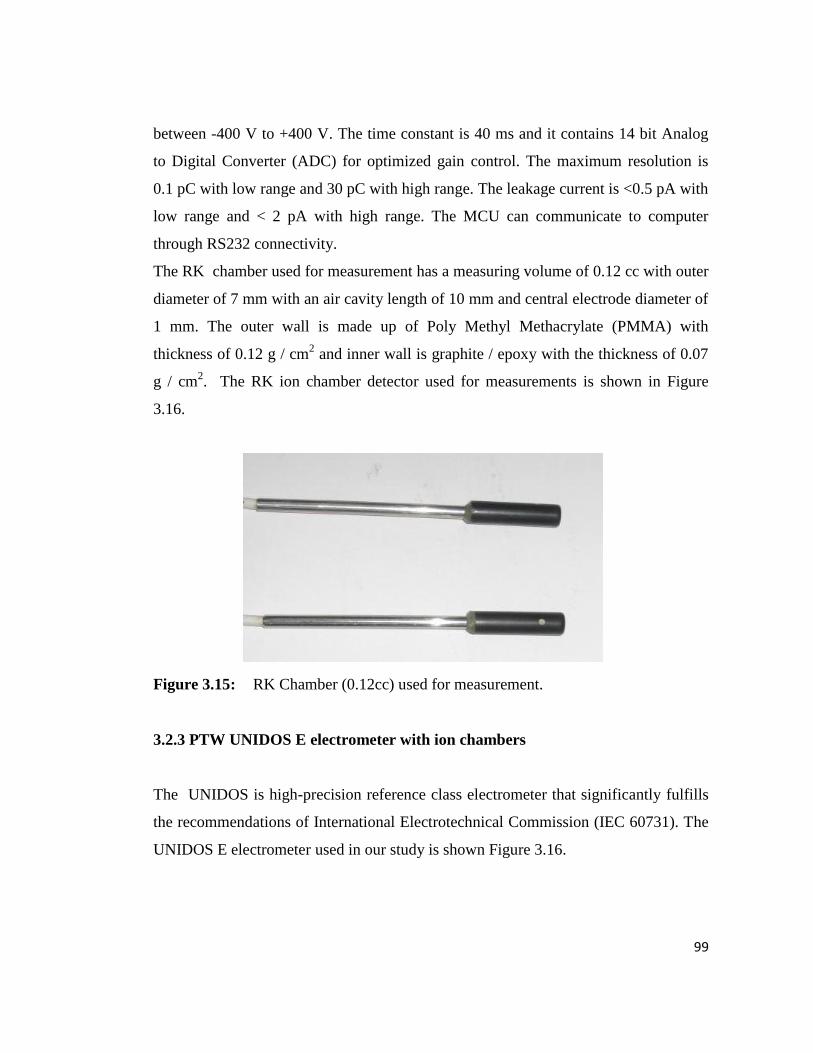
The RK chamber used for measurement has a measuring volume of 0.12 cc with outer

diameter of 7 mm with an air cavity length of 10 mm and central electrode diameter of

1 mm. The outer wall is made up of Poly Methyl Methacrylate (PMMA) with

thickness of 0.12 g / cm2 and inner wall is graphite / epoxy with the thickness of 0.07

g / cm2. The RK ion chamber detector used for measurements is shown in Figure

3.16.

Figure 3.15: RK Chamber (0.12cc) used for measurement.

3.2.3 PTW UNIDOS E electrometer with ion chambers

The UNIDOS is high-precision reference class electrometer that significantly fulfills

the recommendations of International Electrotechnical Commission (IEC 60731). The

UNIDOS E electrometer used in our study is shown Figure 3.16.

100

Figure 3.16: UNIDOS E electrometer

The electrometer has a large and high contrast graphic electro luminescent display

with wide viewing angle for complete and comprehensive display for all measured

values, selected chamber and correction factors in the main screen. It is capable of

displaying the measured dose, dose rate, current, charge, average rate and dose per

monitor unit are all measured and displayed simultaneously. The maximum operating

bias voltage is ± 400 V, programmable in steps of ±50 V. The mains operating power

supply is 90 – 240 V, 50 / 60 Hz, the battery operational is optional. UNIDOS E can

be connected to personal computer through bidirectional Recommended Standard 232

(RS-232) port. The leakage through electrometer is < ±1 fA. The electrometer has a

linearity of < ±0.5% in the whole range. The FC65-G Farmer chamber is a water

proof vented ion chamber suitable for electron and photon beam dosimetry. It‟s

sensitive volume is 0.6 cc. The outer electrode wall material is graphite and the inner

electrode is made up of aluminum. The recommended polarizing voltage is +400 volt

and the leakage < 4 x 10 - 15 A.

101

3.2.4 2D Array detector (PTW Octavius system)

The PTW seven29 2D-Array consists of 729 vented plane-parallel ionization

chambers with a 0.6 g/cm2 graphite wall arranged in a 27 x 27 matrix covering an area

of 27 x 27 cm2 . The 2D array detector used in our study is shown in figure 3.17.

Figure 3.17: Schematic view of PTW Seven29 2D array

Each single chamber is air-filled with a cross section of 5 mm x 5 mm and height of 5

mm. The chambers are separated from each other by 5 mm. The distance between the

centers of adjacent chambers is 10 mm. The 2D array surrounding material is made up

of polymethyl methycrylate (PMMA).

Figure 3.18 PTW Seven29 2D- ARRAY inserted in a Octavious phantom.

102

The measuring system consists of the chamber array itself, which also accommodates

part of the electronic devices, the array interface, and a data acquisition board for the

personal computer. A dedicated phantom for the QA of rotational treatments focusing

primarily on the use of the Seven29 2D ion chamber array, called Octavius was used

during measurements. Octavius is made of polystyrene (physical density 1.04 g/cm3,

relative electron density of 1.00), and is 32 cm wide and has a length of 32 cm. A 30 x

30 x 2.2 cm3 central cavity allows the user to insert the 2D ion chamber array into the

phantom as in figure 3.18. The position of the cavity is such that when the 2D array is

inserted, the plane through the middle of the ion chambers goes through the center of

the phantom. The measurement ranges for 2D array as specified by manufacturer are

200 mGy – 1000 Gy and 500 mGy min-1

to 8 Gy min-1

. The 2D array is calibrated for

absolute dosimetry in a Co - 60 photon beam. An on-site cross calibration factor

correcting for the quality of the beam can be measured and used by the detector

acquisition software. The 2D array was calibrated using a cross-calibration procedure.

In this procedure a known dose was delivered and the response of the central detector

was used to calculate a cross-calibration factor. This factor was applied to the entire

matrix. For planar measurements, the 2D array was set up at an effective depth of 5

cm in solid water (Gammex Inc., Middleton, WI), and with 10 cm solid water

backscatter.

3.2.5 Beam quality specification

Beam quality specification parameters is considered important in determining quality

of a particular beam and are machine specific. Both based on both air kerma standards

and absorbed dose to water standards, have recommended the Tissue-Phantom Ratio

(TPR20,10), as a specifier of the quality of a high-energy photon beam. TPR20,10 is

defined as the ratio of absorbed doses in water on the central axis of the beam at the

depths of 20cm and 10cm, obtained with a constant SCD of 100cm and a 10 x10 cm2

field size at the position of the detector. The parameter TPR20,10 is a measure of the

103

effective attenuation coefficient describing the approximately exponential decrease of

a photon depth-dose curve beyond the Dmax, and more importantly, it is independent of

the electron contamination in the incident beam. The use of dose ratios for specifying

photon beam quality, the nominal accelerator potential was the parameter most

commonly used in photon beam dosimetry. Measured ionization charge or current or

absorbed-dose ratios were first used as a beam quality index in the dosimetry

recommendations of the Nordic Association of Clinical Physicists (NACP).

Other beam quality specifiers have been proposed for photon beam dosimetry which

are, in most cases, related to the depth of maximum absorbed dose and can, therefore,

be affected by the electron contamination at this depth. In addition, the use of

ionization distributions measured with thimble-type ionization chambers is

problematic, as the displacement of phantom material by the detector has to be taken

into account to convert ionization into dose distributions. This is avoided if plane-

parallel ionization chambers are used, but these are not commonly used in photon

beam dosimetry.

3.2.5.1 Quality Index

The purpose of measuring quality index is to ensure that radiation energy has not

changed significantly. By measuring tissue-phantom ratio (TPR) it is possible to

assess the photon beam quality. Three exposures (100 MU each) are made with gantry

angle 0°, SCD 100 cm and FS 10 x 10 cm2 using a calibrated 0.6cc ionization

chamber positioned at the isocentre at depths of 10 and 20 cm in a water phantom. The

ionization ratio at the depth of 20cm to that of 10cm is known as quality index. The

quality index is dependent on beam energy and it increases linearly with photon beam

energy. The measurement was done for both FF and FFF photons (6 and 10MV).

104

3.2.5.2 Percentage Depth Dose at 10 cm (%DD10)

The percentage depth dose value at 10cm in a 10x10cm2 photon beam with a Source

to Surface Distance (SSD ) of 100cm, % DD10 is considered as one of the beam quality

indicator and is endorsed in absolute dose measurement in AAPM TG51 protocol. In

this study, we have analyzed %DD10 for both FF and FFF of 6 and 10MV photon

beams using 0.6cc cylindrical chamber.

3.2.5.3 Depth of dose maximum (Dmax)

Depth of dose maximum (Dmax) depends on the beam energy and beam field size.

Nominal values for Dmax ranges from 0 to 5 cm (orthovoltage Xray beams to 25MV

photon beams). This study presents Dmax for a reference FS 10x10cm2 at SSD 100cm,

for both FF and FFF with 6 and 10MV photon beams.

3.2.6 Beam characteristic

When defining reference parameters of profiles in photon fields, such as flatness,

symmetry , stability and penumbra is an important parameter of influence since the

dose distribution is affected by lateral variations in the beam quality. In megavoltage

photon beams, most of these parameters are commonly specified at 10 cm depth,

corresponding to a typical treatment depth. Moreover, FF are optimized for this depth

and, when measuring profiles at shallow depth, e.g., Dmax, profiles typically exhibit

horns and beam flatness is suboptimal. Without the FF, the lateral dose profiles differ

significantly from the typical flat profiles from conventional linacs that have a FF. The

peak in the profile intuitively associated with FFF beams is pronounced only for

medium to large field sizes and depends on photon beam energy. The higher the

energy, the more pronounced the peak. In order to quantify the magnitude of the peak

of non-flat profiles, the lateral distance from central axis at 90%, 75% and 60% dose

105

points on either side of the beam profile were recorded. Penumbra requires some

special consideration because the conventional definition based on 80%–20% dose

values cannot be applied to FFF beams. In our study, the penumbra is determined

using the inflection point of the profile. For the determination of symmetry, stability of

the beam, field size and penumbra, dose profiles were scanned for a field size (FS) of

20x20 cm2, 10 cm depth and SSD of 100 cm.

3.2.6.1 Output Factor ( Sc,p)

The output factor is defined as the ratio of the absorbed dose for the used collimator

setting to the absorbed dose for the reference or normalization field size for the same

MU. Sc,p were measured with a PTW ionization chamber (0.125cc) and RFA water

phantom. The field size measured from 5 X 5 cm2

to 40 X 40 cm2

and the value were

normalized to the 10 x10 cm2

. The measurement was done for both FF and FFF with

100 cm SSD at Dmax.

3.2.6.2 Scatter Factor ( Sc )

The collimator scatter factor (Sc) is defined as the ratio of the output in air for a given

field to that for a reference field (e.g., 10×10cm2). Sc may be measured with an ion

chamber with a buildup cap of size large enough to provide maximum dose buildup

for the given energy beam. Sc were determined with a PTW ionization chamber (type

31003, volume 0.125 cc) and an in-house polystyrene mini-phantom. Scatter factors

for field sizes (5 X 5 cm2

to 40 X 40 cm2) were normalized to the 10 X 10 cm

2

reference field for FF and FFF beams. The measurement was done for both FF and

FFF with 100cm SCD at 10cm depth for different field sizes.

106

3.2.6.3 Surface dose

The skin dose associated with radiotherapy may be of interest for clinical evaluation or

useful in investigating the risk of late effects. The skin is at risk during radiotherapy

for such effects as erythema, desquamation, and necrosis. The surface dose measured

for collimator settings of 10x10cm2 and 20x20cm

2 and compared with the

corresponding nominal flat beam energy. The measurement done using PTW parallel

plate chamber (PPC40) at 0.5 mm depth with SSD at 100 cm.

3.2.6.4 Symmetry of the beam

Symmetry is defined as the maximum ratio within the flattened region, multiplied

with 100 (IEC 60976 (2007)). The dose profile was acquired for a field size

20x20cm2 at 100 SCD, 10 cm depth using IBA RFA -200. The measurements were

repeated over a period of 9 months to find its stability.

3.2.6.5 Stability of the beam

To quantify the stability of FFF beams, lateral distance from central axis at 90%, 75%

and 60% dose points on either side of the beam profile were recorded. The

measurements were repeated over a period of 9 months to find its consistency. The

profile scan was acquired for 20x20 cm2

FS, SCD 100 cm at 10 cm depth. The

graphical representation quantifying the stability of FFF beam is shown figure 3.19.

107

Figure 3.19 : Diagram showing lateral distances at 90%, 75% and 60% dose points

on the beam profile

3.2.6.6 Field Size

FFF high energy photon beams have radial intensity distribution with high intensity in

the center and progressively falling pattern towards the edge. This is due to the

forward moving nature of high energy photons. In general, field size for FF photon

beams are defined at 50% of intensity level along the central axis. In FFF beam the

108

50% intensity level occurs at high gradient region (sharply descending part) of the

beam profile. Field size for FFF beams does not follow standard definition similar to

FF beams. The geometrical field size was defined by collimator setting and radiation

field size was defined through lateral separation between inflection points (IP) along

the central axis. IP is a point, where the progression of dose deposition changes its

direction geometrically from positive to negative or vice versa. In this study, a simple

physical concept for obtaining IP of FFF beams is proposed. IP calculated with the

new concept was compared with Akima spline interpolation method. The

measurement profile were acquired for collimator field size of 20x20 cm2 with 100cm

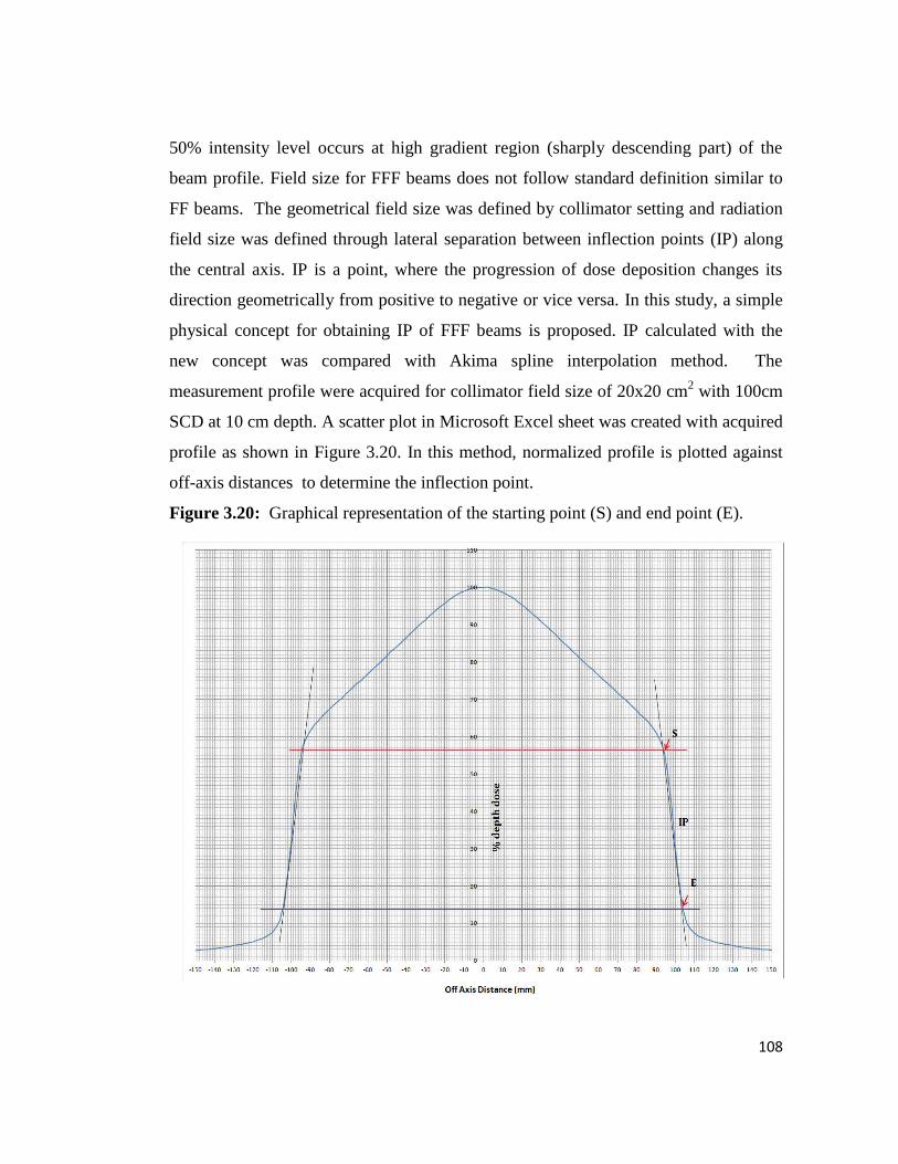
SCD at 10 cm depth. A scatter plot in Microsoft Excel sheet was created with acquired

profile as shown in Figure 3.20. In this method, normalized profile is plotted against

off-axis distances to determine the inflection point.

Figure 3.20: Graphical representation of the starting point (S) and end point (E).

109

The location of starting point (S) and ending point (E) of high gradient region of the

beam profile is described (Figure 3.20). The separation between S and E is the height

(h) of the high gradient region of the beam profile. The mid position of the IP is

located at h/2 from either location (S or E).

To verify our approximation method with mathematical inflection point, we used

Akima Spline Interpolation (ASI) method (InterReg Kroll software, Germany version

2.2.0). It is a special spline which is stable to the outliers. In this study, cubic splines

method was not used since it can oscillate in the neighborhood of an outlier. Figure

3.21 shows the advantage of ASI method.

Figure 3.21: Comparison of Akima Spline and Cubit spline interpolation

110

The cubic spline with boundary conditions is indicated in green-color. On the intervals

which are next to the outlier, the spline noticeably deviates from the given function -

because of the outlier. ASI is indicated in red-color. Compared to the cubic spline, the

ASI is less affected by the outliers. The dose profile (20x20 cm2 FS, 100 SAD, 10 cm

depth) was imported to InterReg software to determine the inflection point. Field size

for a FFF photon beam is the lateral distance between left and right inflection points.

The graphical representation of inflection point determined by the InterReg software

shown in figure 3.22.

Figure 3.22 : Inflection point determined by the InterReg software

111

3.2.6.7 Beam Penumbra

Penumbra requires some special consideration because the conventional definition

based on 80%–20% dose values cannot be applied to FFF beams. In our study , the

penumbra determined from inflection point of the profile. To determine penumbra,

dose value at IP (Mathematical method and manual approximation method) was taken

as Reference Dose Value (RDV). Points Pa and Pb located at 1.6 and 0.4 times of RDV

respectively were identified. The separation between Pa and Pb on either side of the

profile were measured as the penumbra. The penumbra was indicated along central

axis for 6FFF. The measurement profile acquired for field size 20x20cm2

at 100cm

SAD at 10 cm depth. The graphical representation of determination of penumbra is

shown in figure 3.23.

Figure 3.23: Determination of Penumbra.

112

3.2.7 Absolute dosimetry

The International Atomic Energy Agency (IAEA) is an agency in the United Nations

family concerned with the nuclear field. It strives to monitor nuclear technologies and

promote nuclear safety. One of these recommendations is the Technical Report Series

#398 ( TRS398 1990) that is concerned with dose determination based on absorbed

dose to water.

According to IAEA TRS-398, the absorbed dose to water measured with an ionization

chamber is

Dw,Q 0 = MQ0 ND,w,Q0 (Eq.3.20)

In the above formula,MQ0 is the reading of the dosimeter at a standards laboratory, and

ND,w,Q0 is the calibration coefficient obtained for the ionization chamber with respect

to the dosimeter at a standard laboratory at reference beam quality Q0. The calibration

factor is determined in units of μGy/nC. However, equation is only true if conditions

are identical to the conditions at the standards laboratory. This is generally not the

case, which means that some corrections have to be done to compensate for the

differences. The IAEA has a set of factors for the calibration of ionization chambers.

Beam quality factor kQ,Q0 :

The beam quality factor kQ,Q0 is a factor to correct for difference in the ionization

chamber response to the beam quality factor of the user beam Q and reference beam

Q0. It is defined as

(Eq.3.21)

113

For high energy photons with a beam quality Q,KQ,Q0 is specified by the Tissue-

Phantom Ratio TPR20,10 which can be found using the below equation

(Eq.3.22)

where the beam energy E and field size S are held constant. Using a 10 x 10 cm2 field

size and a constant SAD of 100 cm, the absorbed dose is measured at a depth of 10

g/cm2

and then at a depth of 20 g/cm2. From this calculated value of the TPR20,10 a

corresponding beam quality factor KQ,Q0 can be looked up in the table available in the

report. Typically the value for KQ,Q0 ranges from 0.96 to 1.005.

Atmospheric factor KTP :

The gas in the ionization chamber is subject to change with varying temperature and

pressure. Therefore an atmospheric factor KTP, given by below equation, has to be

taken into account if atmospheric conditions are different from the conditions at the

time of calibration.

(Eq.3.23)

where P and T are the pressure and temperature in the chamber at the time of

measurement, while T0 and P0 are the reference conditions of the chamber. The

reference conditions are T0 = 200C and P0 = 101.3 kPa.

114

Ion recombination factor ks :

Some of the ion pairs created inside the chamber volume recombine before they are

registered by the electrodes. The ion recombination factor accounts for this loss

(Eq.3.24)

Where M1 and M2 are the electrometer readouts at V1 and V2 voltage respectively.

Constants a0 , a1 and a2 depend on the value of V1 ,V2 and are retrieved from a table

provided in the report as calculated by Weinhous et al. (1984). Typical values of Ks

range from 1.002 - 1.008.

The ion recombination correction factor, Ks, is defined to account for incomplete

collection of charges and it is a function of dose per pulse in a linear accelerator. Dose

per pulse in the unit of monitor units per pulse (MU/pulse) is dose rate (MU/min)

divided by pulse rate (pulse/min). Since pulse rate of the linear accelerator for the

same nominal energy does not change, Pion becomes a function of the dose rate of the

photon beams. For the FFF X-rays, dose rate increases substantially and hence Ks of

the FFF photons may be different from the conventional flattened photons. Therefore,

ion recombination in the Farmer, PinPoint, or parallel-plate ion chambers may vary in

the FFF beams. The purpose of this study is to evaluate the ion recombination for

typical thimble and plane-parallel chambers in the FFF photon radiation to facilitate

the quality assurance procedure and accurate dose calibrations for the FFF X-rays.

Polarity factor Kp :

This effect is mostly negligible for photon beams, but can b e prominent for charged

particle beams. It is given by

(Eq.3.25)

115

Where M+ and M- are electrometer readings obtained at positive and negative

polarity, respectively. M is the electrometer reading at the routinely used polarity. The

polarity correction was not taken into account for the photon measurements in this

thesis as its effect is assumed to be negligible in photon beams.

In our study , Evaluation of effect for the Farmer, PinPoint, or parallel-plate ion

chambers.

Perturbation factors :

The ionization chamber perturbs the beam due to the cavity inside the chamber, the

chamber wall and the waterproof sleeve. For high energy photon beams in a water

phantom, all of these effects are assumed to b e accounted for in the kQ,Q0 factor.

3.2.8 Beam modeling with AAA for FFF

Before a treatment unit can be put in use, it‟s beam characteristics need to be modeled

accurately in the TPS so that the beam can be reproduced for treatment planning

purposes. The beam model should be general enough to cover all relevant field

shaping techniques and treatment methods, such as 3D-CRT and IMRT. It may also

allow for the possibility to use different dose calculation algorithms, e.g. pencil

kernels and point kernels, or even direct Monte Carlo simulation. For the eclipse

planning system the beam data, including profiles, depth dose curves and output

factors in air and water are collected and modeled for FFF beam.In theory, the

dosimetric characteristic of unflattened beams facilitates dose calculation and might

improve the dose calculation accuracy of advanced algorithms. IMRT, using aperture

based segments with subsequent segment weighting, will benefit from the rather flat

output factor variation with field size.

116

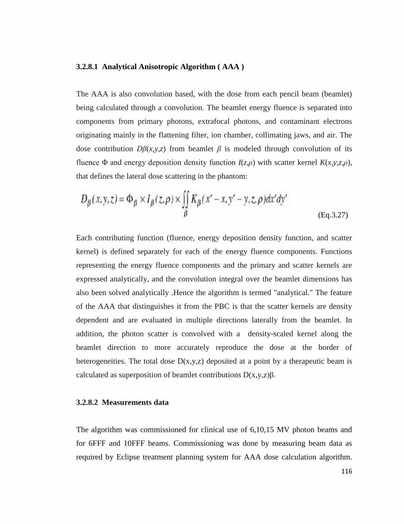
3.2.8.1 Analytical Anisotropic Algorithm ( AAA )

The AAA is also convolution based, with the dose from each pencil beam (beamlet)

being calculated through a convolution. The beamlet energy fluence is separated into

components from primary photons, extrafocal photons, and contaminant electrons

originating mainly in the flattening filter, ion chamber, collimating jaws, and air. The

dose contribution Dβ(x,y,z) from beamlet β is modeled through convolution of its

fluence Φ and energy deposition density function I(z,ρ) with scatter kernel K(x,y,z,ρ),

that defines the lateral dose scattering in the phantom:

(Eq.3.27)

Each contributing function (fluence, energy deposition density function, and scatter

kernel) is defined separately for each of the energy fluence components. Functions

representing the energy fluence components and the primary and scatter kernels are

expressed analytically, and the convolution integral over the beamlet dimensions has

also been solved analytically .Hence the algorithm is termed "analytical." The feature

of the AAA that distinguishes it from the PBC is that the scatter kernels are density

dependent and are evaluated in multiple directions laterally from the beamlet. In

addition, the photon scatter is convolved with a density-scaled kernel along the

beamlet direction to more accurately reproduce the dose at the border of

heterogeneities. The total dose D(x,y,z) deposited at a point by a therapeutic beam is

calculated as superposition of beamlet contributions D(x,y,z)β.

3.2.8.2 Measurements data

The algorithm was commissioned for clinical use of 6,10,15 MV photon beams and

for 6FFF and 10FFF beams. Commissioning was done by measuring beam data as

required by Eclipse treatment planning system for AAA dose calculation algorithm.

117

Machine specific beam data at reference condition were acquired using RFA and other

dosimetric detectors as recommended. Beam data requirements includes PDD, open

beam profiles along cross plane for different field sizes. Smallest field size used for

measurement is 3x3 cm2 and the largest being 40x40cm

2. Moreover, output factors

were also measured by placing the detector at central axis at reference depth.

Additionally, Diagonal profile for the maximum field size 40x40cm2 were also

acquired.

PDD are measured along central axis up to the depth of 30 cm in water. Open beam

profiles are acquired at five different depths ( Dmax, 5,10,20 and 30cm ) and the scan

limit is 35mm beyond 50% dose laterally. Output factors are measured in SSD 95cm

with detector placed at 5cm depth in water deeper than the electron contamination

range. Reference dose in Gy for reference MU at the calibration depth at 10x10 cm2

were measured.

Measurements of profile & PDD for Add-on materials includes MLC transmission

factor for each photon energy, dosimetric leaf gap for modeling of the rounded leaf

edge transmission were also performed.

3.2.8.3 Data Analysis

The analysis of was performed over five regions, as shown in figure 3.24. These

regions are defined below.

Build down (δ1): dose deviation on central axis beyond the depth of

maximum dose (Dmax)

Build-up and penumbra (δ2): dose deviation on central axis before the

depth of Dmax and in penumbra (where dose gradient is larger than 3%

per mm)

Off-axis (δ3): dose deviation in the inner field at off-axis points and

beyond Dmax

118

Tail (δ4): dose deviation in region outside the geometrical beam edges

(less than 7% of the central axis dose)

The percentage difference between measurements and calculations for profile and

PDD is given by

(Eq.3.28)

where Dcalc and Dmeas are the locally calculated and measured doses (absolute for

depth dose curves and relative for profiles). In region δ4, the deviation was determined

with respect to central axis dose as follows,

(Eq.3.29)

Figure 3.24 : Data analysis for Beam modeling parameters

119

3.2.9 Patients specific QA

After patients plan is approved, The plan needs to be verified. This is usually done

through either a composite plan through a field related approach. The patients plan

was transferred to PTW Versoft. The PTW octavius phantom with seven29 array

dector setup as per PTW manual procedure. The senven29 ionization chambers can

sometimes require a warm-up time and/or dose before irradiation.

3.2.9.1 Dose linearity

The dose linearity test was performed by irradiating the detector with 100 MU using a

10 × 10 cm2 field for 6 FFF and 10 FFF under reference conditions. The dose linearity

was evaluated by measuring the array output for deliveries of 10,25,50,75,

100,125,150,175,200,250,300,350,400,450 and 500 MUs for 6 FFF and 10 FFF

photons beams.

3.2.9.2 Dose rate response

The dose linearity test was performed by irradiating the detector with 100 MU using a

10×10cm2 field for 6 FFF and 10 FFF under reference conditions. The dose rate

response was evaluated by measuring the array output for deliveries of 10,25,50,75,

100,125,150,175,200,250,300,350,400,450and 500 for 400 MU/min and

1400MU/min for 6FFF and 2400 MU/min for 10FFF.

3.2.9.3 Gamma analysis 2D

Five patients were used to assess the delivery of treatment plans under typical clinical

conditions. Head and neck IMRT plans using 6 FFF were created with 7 Field. Each

plan was recalculated on a CT dataset of the Octavius phantom using an initial grid

120

spacing of 2.5 mm and then 5 mm. On import into the planning system inhomogeneity

corrections were removed to ensure that no errors were introduced by variations of

Hounsfield units of a static detector/phantom. Following delivery, each plan was

compared to the calculated plans with a 2D global gamma criterion of 3%/3 mm with

a 10% minimum threshold.

3.3 Clinical use of FFF beam in complex treatment

Medulloblastoma is a fast growing tumor of the cerebellum (posterior fossa) that

controls stability, posture, and complex motor functions such as verbal communication

and swallowing. About 400 new patients, primarily children, were diagnosed with

medulloblastoma in the US every year, slightly more often in males than in females. It

is the most common brain tumor in children aged four and younger and the second

most common brain tumor in children aged 5–14 years. Subsequent to surgery,

medulloblastoma is usually treated with CSI. Although radiotherapy had proven

successful, investigators are still looking for new ways to mitigate the potential side

effects of this treatment. Treatment related late complications are usually hearing

disability, declined cognition, cardiomyopathy, cataract formation, retarded growth,

endocrine dysfunction, and second malignancies. Clinicians consider using techniques

such as IMRT and RA that aim to converge beams of radiation directly at the tumor

eventually improving the long term complications free survival. However,

radiotherapy (RT) planning, delivery, and junction dose verification remain exigent

for craniospinal irradiation (CSI) in medulloblastoma patients. Hence investigating the

emerging new RT techniques such as FFF in IMRT and RA on the basis of dose

volume parameters was encouraged to reduce the normal tissue complications.

Conventional two-dimensional planning for CSI involved field shaping using bony

landmarks in X-ray radiographs; later it evolved into CT simulation techniques.

Geometrical field matching was generally followed in such techniques without

computing any dose volume data for the tumor and normal tissues. Modified treatment

121

planning methods were adapted to get better tumor coverage, dose homogeneity, and

conformity. The matching of cranial and spinal fields still poses a problem in adult

patients with larger spinal lengths since it usually exceeds allowable maximum field

size. Helical tomotherapy allows treatment to large cylindrical volumes (40×160 cm2)

that was compromised with the longer BOT. It raises concerns about intrafraction

motion and whole-body integral doses. When the FF was removed from the linear

accelerators head, a marked increase in dose rate up to 1400 MU/min for 6MV and

2400MU/min for 10MV beams is possible. The higher dose rate could make treatment

delivery more accurate, by giving the patient less time to move between setup and

treatment completion. This might be particularly helpful in CSI, where the tissues are

far more mobile than in the cranium. There is no dosimetric comparison between

flattened and unflattened photon beams for CSI. The aim of this study is to determine

the feasibility of using FFF beams in IMRT and RA for CSI in medulloblastoma

patients and to dosimetrically compare it with 3DCRT, IMRT with static segments

(6X SMLC), IMRT with dynamic segments (6X DMLC), Rapid Arc therapy (6X RA)

with FFF IMRT (6F DMLC), and Rapid Arc therapy (6F RA). The Eclipse Planning

System was used in this study for treatment planning.

3.3.1 Target contouring

Patients were CT scanned from the vertex to coccyx in prone position using

immobilization device (Orfit Industries n.v., Belgium) on multislice CT scanner (GE

Healthcare, USA). Axial images of 3mm slice thickness were exported to Mimvista

contouring station (MIMsoftware Inc, USA) where the target volumes (PTV Brain,

PTV Spine) and normal structures were delineated by radiation oncologists as per the

recommended guidelines. PTV spine included the entire spinal canal, including

cerebrospinal extension to spinal ganglia. OARs such as eyes, thyroid, heart, lungs,

esophagus, liver, and kidney were outlined in the axial CT sections. Treatment

planning was performed in Eclipse (Version 11.0; Varian Associates, Palo Alto, CA,

122

USA) treatment planning system (TPS). It is configured for both true beam

millennium 120 multileaf collimator (MLC) and Siemens ARTISTE 160 MLC

treatment units. The range of patients‟ spine length varied from 28.52 cm to 43.75 cm

(median length: 33.4 cm).

A maximum field size of 40 × 40 cm2 can be possible with the 120 millennium MLC

and 160 MLC Artiste machines. AAA was the dose calculation algorithm used for

inverse optimization. We used the CT data set of five randomly selected

medulloblastoma patients (median age:10 yrs), previously treated with conventional

IMRT were used for this retrospective study.

3.3.2 Dose Planning

Conventional 3DCRT plan, 6X_IMRT, 6F_IMRT, 6X_RA, and 6F_RA were iterated

which resulted in six plans for each patient. The total dose prescribed was 28.80Gy in

16 fractions with 1.8Gy per fraction. An evaluation criterion of 98% of the PTV

receiving 100% of the prescription dose and 107% maximum dose was followed as

per our institution protocol. Normal tissue sparing was considered as important as the

tumor coverage.

3.3.2.1 Conformal Photon Beams (3DCRT)

The 3DCRT for CSI comprised three separate treatment plans such as 3d_Brain,

3d_Spine1, and 3d_Spine2. For the whole brain irradiation, 6MV photon beam was

collimated in such a way that the spine field‟s divergence can be easily matched. Spine

1 comprised the region between 2nd

cervical vertebra, 10th

thoracic vertebra and

whereas spine 2 was between 11th

thoracic vertebra and 5th

lumbar vertebra. Spinal

cord treatments were planned with two oblique beam portals 330∘ and 30∘. The 25∘

enhanced dynamic wedges were used to avoid high-dose regions falling beneath the

skin and to improve dose coverage at larger depths. For the three plans, depth from

123

skin where the maximum possible coverage achieved was taken as the reference point

for dose normalization. Plans were summed up in evaluation mode of the TPS to

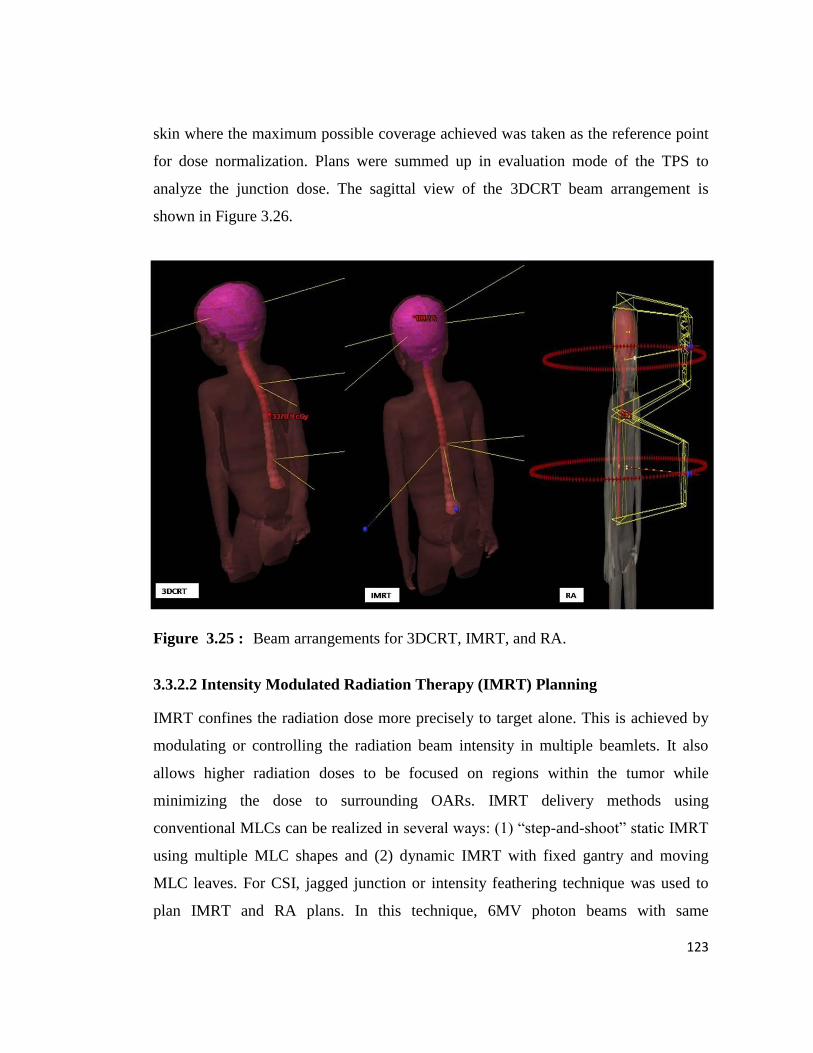
analyze the junction dose. The sagittal view of the 3DCRT beam arrangement is

shown in Figure 3.26.

Figure 3.25 : Beam arrangements for 3DCRT, IMRT, and RA.

3.3.2.2 Intensity Modulated Radiation Therapy (IMRT) Planning

IMRT confines the radiation dose more precisely to target alone. This is achieved by

modulating or controlling the radiation beam intensity in multiple beamlets. It also

allows higher radiation doses to be focused on regions within the tumor while

minimizing the dose to surrounding OARs. IMRT delivery methods using

conventional MLCs can be realized in several ways: (1) “step-and-shoot” static IMRT

using multiple MLC shapes and (2) dynamic IMRT with fixed gantry and moving

MLC leaves. For CSI, jagged junction or intensity feathering technique was used to

plan IMRT and RA plans. In this technique, 6MV photon beams with same

124

optimization can be iterated with multiple isocenters. Thus, summing up of two or

three plans was not needed. The junction evaluation can be avoided which could be a

tedious process involving suitable collimator angles to match dose gradients from the

adjacent field. Since there was no beam matching involved, this treatment technique is

less likely to produce hot or cold spots at the junction, compared to conventional

techniques. Except for one tallest patient, all other cases were planned with two

isocenters and 8 gantry angles. For the tallest of the patients, entire spine was split into

three regions and two separate isocenters apart from the cranial junction were planned

with 12 beam portals. Figure 3.26 shows IMRT beam arrangement. Beam geometry

consisted of four coplanar fields for the whole skull with the gantry angles 225∘,

115∘, 310∘, and 50∘ and upper spine with gantry angles 20∘, 50∘, 340∘, and 310∘. In

case of an additional isocenter for the tallest of all patients, lower spine gantry angles

are 0∘, 30∘, and 60∘. Default smoothing values were used during optimization. To

improve the results, efforts were made to modify constraints and priority factors in

IMRT plans.

3.3.2.3 Rapid Arc Therapy (RA)

RA optimization was performed with version 11.0 from Eclipse (Varian, Palo Alto,

CA, USA). The maximum dose rate (DR) of 600 MU/min for 6X RA and dose rate of

1600MU/Min for 6F RapidArc was selected. All plans were done with 2 isocenters

and 2 full Arcs (179∘–181∘) for each isocenter. These two Arcs were delivered in

opposite rotations (clockwise and counterclockwise). Collimator was set to rotate to a

value other than zero in order to avoid tongue and groove effect. The anisotropic

analytical algorithm (AAA, version 11.00) was the dose calculation algorithm used for

this study.

125

3.3.2.3 Dose-Volume Analysis

Target coverage was quantified with the conformity index (CI) based on International

Commission of Radiation Units report: 50 (ICRU50 1993 ). The dosimetric

parameters such as 𝐷max, 𝐷mean, 𝑉2%, 𝑉98%, 𝑉95%, and 𝑉107% were evaluated for the six

planning techniques. The volumes of each OAR receiving >80% (high; 𝑉80%), >50%

(intermediate; 𝑉50%),>30% (low; 𝑉30%), and >10% (low; 𝑉10%) of the prescribed dose

were extracted from the DVH and compared among the techniques. The techniques

were evaluated for average total BOT.