Chapter 13 INSTRUCTOR GUIDE Pliocene Warmth: Are · PDF fileChapter 13 INSTRUCTOR GUIDE....

Ch 14 Pliocene Warmth: Are We Seeing Our Future? Instructor Guide

of 24

Chapter 13 INSTRUCTOR GUIDE Pliocene Warmth: Are We Seeing Our Future?

SUMMARY The Pliocene Epoch (5.3–2.6 Ma) represents a time interval immediately preceding the growth of large continental ice sheets in the Northern Hemisphere and cyclical glacial–interglacial cy-cles. There is abundant evidence that early to mid-Pliocene time (approximately 5–3 Ma) was warmer and global sea level was higher than today. In addition, plate configurations, moun-tain belts, and ocean circulation were more like today than any other time in the Earth’s his-tory. For these reasons, paleoclimatologists are very interested in studying the Pliocene as a possible analog for the evolving trends of global warming today. In Part 13.1, you will con-sider evidence for global warmth and the role of greenhouse gases in causing this warmth, specifically carbon dioxide (CO2). In Part 13.2, you will consider the magnitude of sea level change during the early to mid-Pliocene, and compare this with ongoing sea level rise today.

FIGURE 13.1. Pliocene paleogeography of North America (left), and modern geography (right). From Dr. Ron Blakey: http://jan.ucc.nau.edu/~rcb7/ Goal: to evaluate the Pliocene as a possible analog for the evolving climate trends of global warming today. Objectives: After completing this exercise, your students should be able to:

1. Describe the paleogeography, climate (the mean annual temperature, latitu-dinal temperature gradient, ice volume, pCO2), and sea level of the early to mid-Pliocene time (approximately 5–3 Ma).

2. Identify what region(s) of the world appear most sensitive to climate forcings and explain why.

3. Differentiate between eustatic and regional sea level, and explain why eustatic and regional rates of sea level change can differ.

http://jan.ucc.nau.edu/~rcb7/�


of 24

4. Discuss the pros and cons of the early to mid-Pliocene as an analog for the evolving trends of global warming today.

I. How Can I Use All or Parts of this Exercise in my Class? (based on Project 2061 instructional materials design.) Part 1 Part 2

Title (of each part) The Last 5 Million Years Sea Level Past, Present & Future

How much class time will I need? (per part)

1 hour 1 hour

Can this be done independently (i.e., as homework

Yes, but should follow-up with class discussion.

Yes, but should follow-up with class discussion.

What content will students be introduced to in this exercise? Science as human endeavour X Science as an evolving process/nature of Science

X

Earth history archives Stratigraphic principles X Climate models X Ocean circulation and sea level changes X Climate changes (it is not static): X X

climate change on human timescales X regional to global scales of change X X

What types of transportable skills will students practice in this exercise? Analysis of authentic data: X X

Making observations X X Recognizing trends and patterns X X

Interpret graphs, diagram, and tables X X Make hypotheses or predictions X

Synthesize, integrate and draw broad conclusions

X X

Math integration: perform calculations and develop quantitative skills

X

Oral and Written Communication X X Recognize and work with uncertainty in data

X X

What general prerequisite knowl-edge & skills are required?

Basic knowledge of stable oxygen isotopes (see be-low)

Calculating rates, convert-ing units.

What Anchor Exercises (or Parts of Exercises) should be done prior to this to guide student interpretation & reasoning?

Completion of Ch 6 (or some knowledge of stable oxygen isotopes), would support questions 1-3, and 5. Completion of Ch 13 on the Plio-Pleistocene Antartic core lithology, would support question 4.

Ch 13 Part 1. Also ques-tions 1 and 2 should rein-force what students learned about the relationship be-tween glacial interglacial cycles and stable benthic oxygen isotopes from Ch 8 part 1 questions 8-13.

What other resources or materials do I need? (e.g., internet access to show on-line video; access to maps, colored pencils)

Internet access for ques-tion 14.

Calculator for question 9.


of 24

What student misconception does this exercise address?

Misconception that atm CO2 levels today are the highest Earth has ever experienced.

Misconception that sea level rise is uniform globally.

What forms of data are used in this? (e.g., graphs, tables, photos, maps)

Graphs, maps Graphs, maps, tables

What geographic locations are these datasets from?

Global, McMurdo Sound Antarctica, Canadian Arctic

Global

How can I use this exercise to iden-tify my students’ prior knowledge (i.e., student misconceptions, com-monly held beliefs)?

Part 1 question 1 helps identify student’s attention to detail and geographic knowledge. Part 1 questions 2-4 and 5 help identify the ability to apply what they learned from Ch 6, and question 4 helps identify their ability to synthesize data. Part 1 question 15 helps iden-tify students’ prior knowledge of CO2 levels today com-pared to the past. In Part 2 questions 6, 7, 10, and 11 will draw out students’ prior knowledge.

How can I encouraging students to reflect on what they have learned in this exercise? [Formative Assess-ment]

Exercise Parts can be concluded by asking: On note card (with or without name) to turn in, answer: What did you find most interesting/helpful in the exercise we did above? Does what we did model scientific practice? If so, how and if not, why not? What did you learn that was new for you or a reinforcement of what you already knew?

How can I assess student learning after they complete all or part of the exercise? [Summative Assess-ment]

See suggestions in Summative Assessment section be-low.

Where can I go to for more informa-tion on the science in this exercise?

See the Supplemental Materials and reference sections below.

II. Annotated Student Worksheets (i.e., the ANSWER KEY)

This section includes the annotated copy of the student worksheets with answers for each Part of this Chapter. This instructor guide contain the same sections as in the student book chap-ter, but also includes additional information such as: useful tips, discussion points, notes on places where students might get stuck, what specific points students should come away with from an exercise so as to be prepared for further work, as well as ideas and/or material for mini-lectures. Pliocene Warmth: Are We Seeing Our Future? Part 13.1. The Last 5 Million Years 1 What’s different about the Pliocene paleogeographic reconstruction (Figure 13.1, left panel), compared with the modern geography (Figure 13.1, right panel)? List ten things that are dif-ferent.

The responses will depend in part on how familiar students are with names for geo-graphic place. You may want them to look up the names of locations (e.g., Spitsber-gen). However they should include these general observations. Specific examples of


of 24

these will easily add up to 10 differences.

• not as much ice cover in the Pliocene (e.g., Greenland, Iceland, Spitsbergen)

• more vegetation in Pliocene (note darker green colour on the mid-continent)

• sea level was higher during the Pliocene (note southern Florida, Hudson Bay, Ire-land, Scotland, Eurasian Arctic shelf, continental shelf around Newfoundland)

• Much fewer lakes in Pliocene (e.g., Great Lakes, and other lakes in the Canadian

shield)

• Fewer islands in Pliocene; more contiguous landmasses (e.g, Canadian Arctic, Newfoundland, Caribbean)

• Possibly more carbonate platforms around Florida and the northeast of South

America

• Possibly more or larger rivers draining into the Gulf of Mexico in Pliocene THE DEEP-SEA BENTHIC FORAMINIFERAL OXYGEN ISOTOPE RECORD In Chapter 6, you were introduced to the δ18O record from benthic foraminifera as a global proxy for seawater temperature and ice volume. In Chapter 8, you identified orbitally driven cycles in these (and other) data and calculated the resulting periodicities. Explore the benthic foraminiferal δ18O record further by examining Figure 13.2 below and an-swering Questions 2–5.

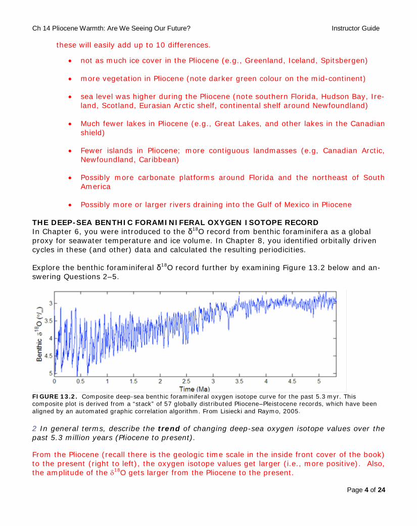
FIGURE 13.2. Composite deep-sea benthic foraminiferal oxygen isotope curve for the past 5.3 myr. This composite plot is derived from a “stack” of 57 globally distributed Pliocene–Pleistocene records, which have been aligned by an automated graphic correlation algorithm. From Lisiecki and Raymo, 2005.

2 In general terms, describe the trend of changing deep-sea oxygen isotope values over the past 5.3 million years (Pliocene to present).

From the Pliocene (recall there is the geologic time scale in the inside front cover of the book) to the present (right to left), the oxygen isotope values get larger (i.e., more positive). Also, the amplitude of the δ18O gets larger from the Pliocene to the present.


of 24

3 The pattern of deep-sea oxygen isotope values shows some distinct differences in fre-quency and amplitude during the past 5.3 million years. Frequency refers to the number of repeated events (cycles) in a certain period of time, whereas amplitude refers to the magni-tude of the changing δ18O values. Characterize the frequency and amplitude of the δ18O data for the following times. Record your answers in the table below.

Time Frequency Amplitude ~1 Ma to the present

Less frequent. 11 cycles

∆δ18O of 1.5-2‰ largest amplitude

3 to ~1 Ma

More frequent. ~44 cycles

∆δ18O 1-1.5‰ large amplitude

~5 Ma to 3 Ma Most frequent.

~44 cycles (but very difficult to count)

∆δ18O ~0.5‰ smallest amplitude

4 If climate change influenced both the deep-sea benthic foram oxygen isotope record (Fig-ure 13.2) and the Antarctic sedimentary record from the McMurdo Sound area (Chapter 12, Figure 12.7), these two datasets should show some similarities. Compare these two records.

(a) How does the up-core general change in lithology in ANDRILL 1-B during the Pliocene and Pleistocene compare with the global trend in δ18O during this time?

This is a great opportunity to have students to compared different datasets from differ-ent location, as well as integrate what they learned in a previous unit with this unit. Be-low is part of figure 12.7 with relevant annotations. You will need to point out to stu-dents which part of the stratigraphic column in Figure 12.7 is the Pleistocene and which is the Pliocene b/c the student version of Figure 12.7 is unfortunately missing the Plio-cene label in the left hand column. The main observation is that: as the global δ18O trend gets more positive, the ANDRILL 1-B lithology becomes dominated by glacial tills. In both the Pliocene and Pleistocene however we see repeated lithologies (cycles), just as we do in the global δ18O record.


of 24

(b)

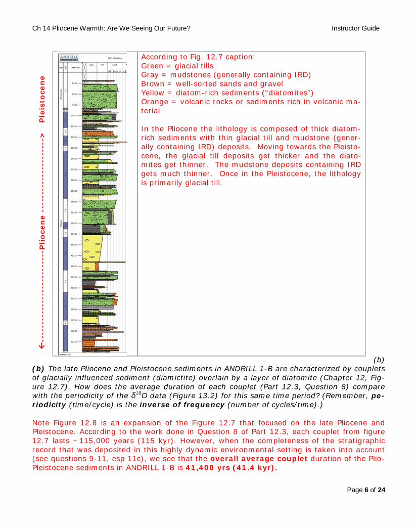
(b) The late Pliocene and Pleistocene sediments in ANDRILL 1-B are characterized by couplets of glacially influenced sediment (diamictite) overlain by a layer of diatomite (Chapter 12, Fig-ure 12.7). How does the average duration of each couplet (Part 12.3, Question 8) compare with the periodicity of the δ18O data (Figure 13.2) for this same time period? (Remember, pe-riodicity (time/cycle) is the inverse of frequency (number of cycles/time).) Note Figure 12.8 is an expansion of the Figure 12.7 that focused on the late Pliocene and Pleistocene. According to the work done in Question 8 of Part 12.3, each couplet from figure 12.7 lasts ~115,000 years (115 kyr). However, when the completeness of the stratigraphic record that was deposited in this highly dynamic environmental setting is taken into account (see questions 9-11, esp 11c), we see that the overall average couplet duration of the Plio-Pleistocene sediments in ANDRILL 1-B is 41,400 yrs (41.4 kyr).

According to Fig. 12.7 caption: Green = glacial tills Gray = mudstones (generally containing IRD) Brown = well-sorted sands and gravel Yellow = diatom-rich sediments (“diatomites”) Orange = volcanic rocks or sediments rich in volcanic ma-terial In the Pliocene the lithology is composed of thick diatom-rich sediments with thin glacial till and mudstone (gener-ally containing IRD) deposits. Moving towards the Pleisto-cene, the glacial till deposits get thicker and the diato-mites get thinner. The mudstone deposits containing IRD gets much thinner. Once in the Pleistocene, the lithology is primarily glacial till.

--

----

----

----

----

----

----

Plio

cen

e -

----

----

----

----

----

>

Ple

isto

cen

e


of 24

To determine the periodicity of the of the δ18O data (Figure 13.2) for this same time period, we can turn to Figure 13.2 and the answer to Part 13.1 question 3. Recall too that Plio-Pleistocene boundary is at 2.6 Ma (see inside front cover of book for time scale). Therefore, we will use the 1-3 Ma data from Part 13.1 question 3, which has ~44 cycles over a ~2 Ma period so... 44 cycles/2 Ma = 22 cycles/Ma But, that is the frequency and we want to determine the periodicity, which is the inverse of the above (this is pointed out to students at the end of question 4b, and was address also in the introduction to Ch 8). So the periodicity is: 1 Ma/22 cycles = 0.045 Ma/cycle And converting to kyr: 0.045 Ma/cycle x 1000 kyr/1Ma = 45 kyr These are fairly similar even though they are from different datasets and location. Both reflect the strong obliquity influence on climate during this time. For more information on obliquity see Ch 8 Part 8.2. THE PLIOCENE RESEARCH, INTERPRETATION AND SYNOPTIC MAPPING (PRISM) PROJECT Data analysis and climate modelling are used to estimate past temperatures. Estimates of global warming during the mid-Pliocene Epoch, early Piacenzian Age (Figure 13.3, shaded in-terval: 3.264–3.025 Ma) suggest that global mean annual temperatures were 2°C warmer than today. The Intergovernmental Panel on Climate Change (IPCC) report of 2007 has predicted that a 2°C warming during the 21st century (i.e., this century) falls within the range of likely global warming in the coming decades (see Chapter 7, Part 7.1). If true, in this century, global average temperatures could reach values, which have not been experi-enced since the mid-Pliocene. The Pliocene Research, Interpretation and Synoptic Map-ping group (PRISM) of the US Geological Survey is a project to understand global warming in the Earth’s recent past under conditions with similar plate configurations, paleogeography, and ocean circulation. Numerical simulations are designed to understand the sensitivity, cli-matic impact, and feedbacks forced by future global warming. Data thus far suggest that Plio-cene warmth was the consequence of elevated greenhouse gases and increased ocean heat transport, together with associated, but yet unresolved, feedback in the ocean–climate system. From: http://geology.er.usgs.gov/eespteam/prism/index.html

http://geology.er.usgs.gov/eespteam/prism/index.html�


of 24

FIGURE 13.3. Geomagnetic polarity time scale and deep-sea benthic foraminiferal oxygen isotope data for the Pliocene Epoch from Lisiecki and Raymo (2005). The shaded interval in the mid-Pliocene is being studied in detail by the Pliocene Research, Interpretation and Synoptic Mapping group (PRISM) of the US Geological Survey (see box above). Note: the International Commission on Stratigraphy has recently moved the Pliocene/Pleistocene Epoch boundary down to the Piacenzian/Gelasian Age boundary (2.6 Ma). The vertical line at approximately 3.2‰ (per mil) δ18O represents present-day oxygen isotope values in the deep-sea.


of 24

5 The vertical line at approximately 3.2‰ (per mil) δ18O represents present day oxygen iso-tope values in the deep-sea. What can we infer about temperature and ice volume during early to mid-Pliocene time compared to today? Are they warmer or colder? Is there less ice or more ice? Explain. The δ18O values ranged from 2.8‰ in early Pliocene to about 3.2‰ by the mid-Pliocene. These values are similar to (3.2‰) or lower (2.8‰) than the modern-day oxygen isotope value. We know from earlier exercises (see Ch 5 Part 5.4 on Greenhouse and Icehouse worlds and Ch 10 on Antarctic glaciation) that that glaciers and ice sheets were present at least in Antarctica since the Oligocene, and we know that glaciers and ice sheets exist today. There-fore it is reasonable to assume that the variation in δ18O values during the Pliocene reflect ice-volume changes in addition to temperature changes. Because the early to mid-Pliocene δ18O values were lower than today we can infer that the early to mid-Pliocene was warmer and had less ice than today. FIGURE 13.4. Modern mean annual sea surface temperature (SST). The Western Pacific Warm Pool (WPWP) is the large pod of 30°C water in the tropical western Pacific and eastern Indian Ocean. From Dowsett and Robinson, 2009. FIGURE 13.5. Pliocene reconstruction map (PRISM3) of mean annual sea surface temperature (SST) based on numerical data and climate modeling. This study focused on the tropical Pacific. From Dowsett and Robinson, 2009.


of 24

6 Compare modern mean annual SST (Figure 13.4) with estimated mid-Pliocene mean annual SST (Figure 13.5). List five differences between the two SST maps:

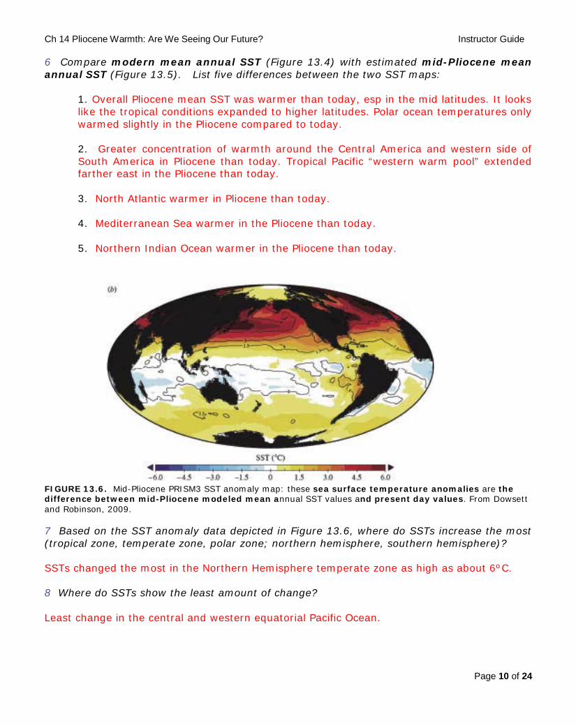
1. Overall Pliocene mean SST was warmer than today, esp in the mid latitudes. It looks like the tropical conditions expanded to higher latitudes. Polar ocean temperatures only warmed slightly in the Pliocene compared to today. 2. Greater concentration of warmth around the Central America and western side of South America in Pliocene than today. Tropical Pacific “western warm pool” extended farther east in the Pliocene than today. 3. North Atlantic warmer in Pliocene than today. 4. Mediterranean Sea warmer in the Pliocene than today. 5. Northern Indian Ocean warmer in the Pliocene than today.

FIGURE 13.6. Mid-Pliocene PRISM3 SST anomaly map: these sea surface temperature anomalies are the difference between mid-Pliocene modeled mean annual SST values and present day values. From Dowsett and Robinson, 2009. 7 Based on the SST anomaly data depicted in Figure 13.6, where do SSTs increase the most (tropical zone, temperate zone, polar zone; northern hemisphere, southern hemisphere)? SSTs changed the most in the Northern Hemisphere temperate zone as high as about 6ºC. 8 Where do SSTs show the least amount of change? Least change in the central and western equatorial Pacific Ocean.


of 24

The above study (Dowsett and Robinson, 2009; Figures 13.4–13.6) focused on sea surface temperatures (SSTs) during the mid-Pliocene. Next, we will consider data from an early Plio-cene peat deposit in the high Canadian Arctic. Peat is a sedimentary deposit rich in decaying terrestrial organic matter and forms in bogs, marshes, and wetlands. Ballantyne et al. (2010; Figure 13.7) estimated mean annual (air) temperature (MAT) for the early Pliocene using multiple proxies for the early Pliocene: (a) oxygen isotopes of fossil wood cellulose and annual tree ring widths, (b) coexistence of paleovegetation, and (c) bacterial tetraether composition in paleosols (ancient soils). The MAT estimates from the three proxies are statistically indis-tinguishable and are plotted together in Figure 13.7 (black filled circles within red oval). The peat deposit provides the highest latitude terrestrial estimates of paleotemperature for the early Pliocene and anchors the northern end of this latitudinal (i.e., meridional) MAT gradient.

FIGURE 13.7. (a) Latitudinal mean annual temperature (MAT) gradients of the past (early Pliocene, solid black line; and early Eocene, dashed black line) compared with the present (Modern; gray line). The three independent temperature estimates from the high Canadian Arctic peat deposit are shown as filled black circles with standard error bars (within red oval). (b) Difference between present day MAT gradient and early Eocene (dashed black line) and early Pliocene (solid black line). 90 = North Pole, −90 = South Pole, 0 = Equator. From Ballantyne et al., 2010.

9 The consequence of global warming of the past can be seen by examining the early Plio-cene latitudinal temperature gradient (solid black line; Figure 13.7). During the early Plio-cene, what latitudes experienced the greatest deviation from modern MAT tempera-tures (i.e., what regions of the planet were most sensitive to rising temperatures during the early Pliocene)? The poles.

10 How much warmer were mean annual temperatures in the Arctic during the early to mid-Pliocene compared with today?


of 24

According to Figure 13.7, the Arctic was ~15 to 18ºC warmer during the early Pliocene than today!

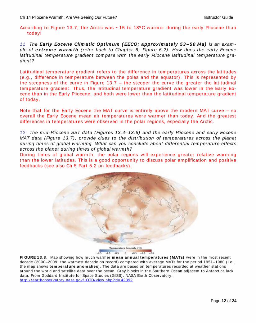
11 The Early Eocene Climatic Optimum (EECO; approximately 53–50 Ma) is an exam-ple of extreme warmth (refer back to Chapter 6; Figure 6.2). How does the early Eocene latitudinal temperature gradient compare with the early Pliocene latitudinal temperature gra-dient? Latitudinal temperature gradient refers to the difference in temperatures across the latitudes (e.g., difference in temperature between the poles and the equator). This is represented by the steepness of the curve in Figure 13.7 – the steeper the curve the greater the latitudinal temperature gradient. Thus, the latitudinal temperature gradient was lower in the Early Eo-cene than in the Early Pliocene, and both were lower than the latitudinal temperature gradient of today. Note that for the Early Eocene the MAT curve is entirely above the modern MAT curve – so overall the Early Eocene mean air temperatures were warmer than today. And the greatest differences in temperatures were observed in the polar regions, especially the Arctic. 12 The mid-Pliocene SST data (Figures 13.4–13.6) and the early Pliocene and early Eocene MAT data (Figure 13.7), provide clues to the distribution of temperatures across the planet during times of global warming. What can you conclude about differential temperature effects across the planet during times of global warmth? During times of global warmth, the polar regions will experience greater relative warming than the lower latitudes. This is a good opportunity to discuss polar amplification and positive feedbacks (see also Ch 5 Part 5.2 on feedbacks). FIGURE 13.8. Map showing how much warmer mean annual temperatures (MATs) were in the most recent decade (2000–2009; the warmest decade on record) compared with average MATs for the period 1951–1980 (i.e., the map shows temperature anomalies). The data are based on temperatures recorded at weather stations around the world and satellite data over the ocean. Gray blocks in the Southern Ocean adjacent to Antarctica lack data. From Goddard Institute for Space Studies (GISS), NASA Earth Observatory: http://earthobservatory.nasa.gov/IOTD/view.php?id=42392

http://earthobservatory.nasa.gov/IOTD/view.php?id=42392�


of 24

13 How do these ancient trends of temperature change (early Pliocene and early Eocene) com-pare with the modern trends of global warming shown in Figure 13.8? The modern, early Pliocene, and early Eocene Northern Hemisphere higher latitude regions are warmed more than low latitudes. And the Southern Hemisphere is not as affected as mcu as the Northern Hemisphere. Also see Ch 7 Part 7.1 question 6 and figure 7.3) to compare the modern, and paleo-temperature model results discussed here, with model results of future temperature change across the globe; again, there are strong similarities. Note too that the models display some differences between the modern Arctic warming com-pared to the Pliocene warm period. In the modern (Figure 13.8) the Arctic region is warmed the most whereas in the Pliocene (Figure 13.6), subpolar (subarctic) region is warmed more than the Arctic. (This may be explained, in part, by limited sample resolution in the Arctic for the Pliocene reconstruction.)

Atmospheric Carbon Dioxide and Global Climate As we have seen in previous exercises, the concentration of greenhouse gases in our atmos-phere, such as carbon dioxide (CO2) and methane (CH4), play a primary role in controlling mean annual temperatures across the planet (see Chapters 5, 9, and 10). 14 What is the concentration of CO2 in the atmosphere today? A good source for up-to-date trends in atmospheric CO2 is http://www.esrl.noaa.gov/gmd/ccgg/trends/

~396 ppm (in 2012) 15 As a first approximation, what do you predict the concentration of CO2 was like during the early to mid-Pliocene relative to today: much higher, somewhat higher, the same, somewhat lower, much lower? This is a good way to gauge students’ prior understanding (if you can keep them looking ahead to the data plotted in Fugre 13.9). Based on the work they’ve done in Ch 13 thus far, (seeing the data supporting a warm early to mid-Pliocene, and the text in the Box on page 434), and knowing the basic relationship between pCO2 and temperature (see Ch 5), student will likely respond that pCO2 levels were probably higher during the early to mid-Pliocene than they are today. Review the data presented in Figure 13.9 below and answer the questions that follow.

http://www.esrl.noaa.gov/gmd/ccgg/trends/�


of 24

FIGURE 13.9. Estimates of Pliocene–Pleistocene atmospheric concentration of carbon dioxide [pCO2 (ppm)] at six different ODP sites (a–f) calculated from alkenone carbon isotope fractionation (εp) and phosphate (PO4

3–) proxies. Upper and lower pCO2 estimates show a calculated range of values based on depth in photic zone (0 to 75 m) of the coccolithophorids (phytoplankton) responsible for the alkenone biomarkers used in this study. The dashed lines are linear regressions of maximum and minimum CO2 estimates. From Pagani et al., 2009. 16 Describe the general trend of atmospheric CO2 from the early Pliocene to the present (Figure 13.9).

Note: age scale goes from right to left, older to younger. The general trend of atmospheric CO2 decreases towards the present (towards 0.5 Ma).

17 Draw a horizontal line on each of the six plots in Figure 13.9 showing present day pCO2 values (see your answer to Question 14). How do early and mid-Pliocene estimated values of pCO2 compare with modern values?

Red horizontal lines are plotted. Note that for 13.9f the line is well above the graph because 396 ppm is off the vertical scale. It would be interesting to plot these 6 sites on a map to determine the regional variability. See the instructor guide in Ch 2 for how to access the GoogleEarth IODP site map, which students could use to find the locations of these 6 sites.

The question asks to compare modern values to those during the early to mid-Pliocene, so

students should focus on the values between 3 and 5 Ma for the early to mid-Pliocene val-ues. Estimated values of pCO2 during the early to mid-Pliocene were similar to or lower than the modern pCO2 value.


of 24

18 What take-away messages do you glean from these Pliocene data relative to present day pCO2 values?

The PRISM data suggests that the early to mid-Pliocene was warmer than today, but the pCO2 levels were similar to or lower than today. These data suggest that the early to mid-Pliocene, climate was highly sensitive to changes in pCO2 – a little change in pCO2 could result is a large

change in atmospheric temperature. In addition, while elevated pCO2 levels are an important driver of global warming, it is NOT the ONLY driver of global warming – other influences (e.g, positive feedbacks, changes in ocean circulation, increase in other greenhouse gases besides CO2) must also be playing a role to augment the pCO2 effect on temperature.

Part 13.2. Sea Level Past, Present, and Future

Onset of Northern Hemisphere Glaciation

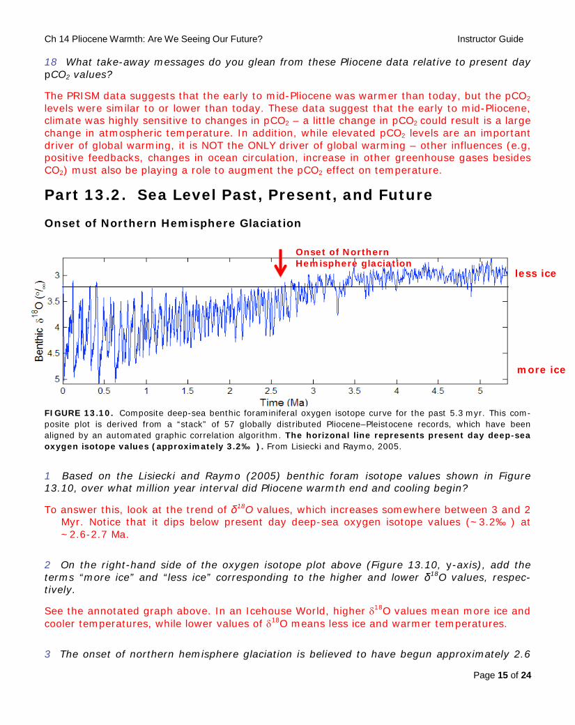
FIGURE 13.10. Composite deep-sea benthic foraminiferal oxygen isotope curve for the past 5.3 myr. This com-posite plot is derived from a “stack” of 57 globally distributed Pliocene–Pleistocene records, which have been aligned by an automated graphic correlation algorithm. The horizonal line represents present day deep-sea oxygen isotope values (approximately 3.2‰). From Lisiecki and Raymo, 2005.

1 Based on the Lisiecki and Raymo (2005) benthic foram isotope values shown in Figure 13.10, over what million year interval did Pliocene warmth end and cooling begin?

To answer this, look at the trend of δ18O values, which increases somewhere between 3 and 2 Myr. Notice that it dips below present day deep-sea oxygen isotope values (~3.2‰) at ~2.6-2.7 Ma.

2 On the right-hand side of the oxygen isotope plot above (Figure 13.10, y-axis), add the terms “more ice” and “less ice” corresponding to the higher and lower δ18O values, respec-tively.

See the annotated graph above. In an Icehouse World, higher δ18O values mean more ice and cooler temperatures, while lower values of δ18O means less ice and warmer temperatures.

3 The onset of northern hemisphere glaciation is believed to have begun approximately 2.6

less ice

more ice

Onset of Northern Hemisphere glaciation


of 24

Ma based on the occurrence of ice-rafted debris in the deep-sea of the northern high lati-tudes, the deep-sea benthic foram record, such as that of Lisiecki and Raymo (2005), and other proxy records (see Chapter 14). With a vertical arrow, mark the point on the Lisiecki and Raymo oxygen isotope curve (Figure 13.10) corresponding to the onset of northern hemi-sphere glaciation. See red arrow on figure 13.10. 4 Changes in ice volume and water temperature can affect the oxygen isotopic composition of deep-sea benthic forams. If the difference between early to mid-Pliocene deep-sea benthic foram δ18O values and those of today (approximately 3.2‰; Figure 13.10) is based solely on ice volume differences and not on changes in deep water temperatures, we can estimate the corresponding change in sea level (since changes in ice volume directly affect sea level). Ap-proximately how different was early to mid-Pliocene sea level compared with today, if 0.11‰ = 10 m of sea level? Show your work. Given that: 0.11‰ = 10 m of sea level, and today δ18O = ~3.2‰ then: 0.11‰/10m = 3.2‰/X X = 3.2‰/0.11‰ × 10 m X = 290.91 m Similarly, given that 0.11‰ = 10 m of sea level, and the early to mid-Pliocene (3 to 5 Ma) δ18O = ~2.8‰ (from question 5 in Part 31.1, or inferred from the graph in Figure 13.10), then: 0.11‰/10m = 2.8‰/X X = 2.8‰/0.11‰ × 10 m X = 254.55 m Therefore, the difference between mid-Pliocene and modern sea level: 290.91 m - 254.55 m = 36.36 m. Therefore the mid-Pliocene sea level was ~36 m higher than today.

5 Based on Figure 13.11, describe the nature of global sea level change since the Pliocene.

Sea level was higher during the Pliocene than today. The mid-Pliocene coastline is marked by light green, and the modern coast line by dark green in Figure 13.11. Therefore during the Pliocene the dark green region would have been flooded (below sea level). It also appears that the eastern coasts of the US and the Gulf of Mexico region were affected by sea level change more so than the islands (e.g., Cuba). This may reflect the slope of the coastal zone in these regions, with more gently sloping (passive margins) along the eastern coasts of the US and Gulf of Mexico regions than along the volcanic and carbonate bank islands.


of 24

FIGURE 13.11. Map of the US East Coast, Gulf Coast, Gulf of Mexico and northern Caribbean depicting the changes in global (eustatic) sea level since the Pliocene. The light blue color shows the area exposed by low-ered sea level during the Last Glacial Maximum (LGM), about 18,000 years ago (18 ka). During the LGM, the continental shelves were completely exposed as sea level fell approximately 125 m (approximately 410 ft.). The dark green color shows the approximate area flooded during the global warmth and related sea level rise of the mid-Pliocene (+35 m), about 3 million years ago. From http://geochange.er.usgs.gov/data/sea_level/ofr96000.html Reproduced with the permission of Peter Schweitzer and Robert Thompson.

6 Is sea level expected to remain static over time?

Obviously not; figure 13.11 is a nice regional example of the changing sea level, since it shows coastlines for 3 time periods: mid-Pliocene, late-Pleistocene (last glacial maximum), and today.

7 What is the principal mechanism that controls global sea level?

The principal mechanism is changes in ice volume (and secondarily changes in sea water temperature since water expands as it gets warmer). All land based ice melt contributes to sea level rise. And the greater the volume of ice, the greater the potential sea level rise should that ice (e.g., ice sheets) melt. However don’t dis-count the small volume glaciers as being significant, and early, contributors to sea level rise during times of global warming. In fact, although glaciers make up a smaller total ice volume than do ice sheets, their faster response time to climate forcing means the glaciers contribute a larger present of the ice melt contribution to recent sea level rise. According to Meier et al., (2007), “the network of lower latitude small glaciers and ice caps, although making up only about four percent of the total land ice area or about 760,000 square kilometers, may have provided as much as 60 percent of the total glacier contribution to sea level change since 1990s” (http://nsidc.org/cryosphere/sotc/sea_level.html, referencing Meier, M.F., M.B. Dyur-gerov, U.K. Rick, S. O'Neel, W.T. Pfeffer, R.S. Anderson, S.P. Anderson, and A.F. Glazovsky.

http://geochange.er.usgs.gov/data/sea_level/ofr96000.html�

http://nsidc.org/cryosphere/sotc/sea_level.html�


of 24

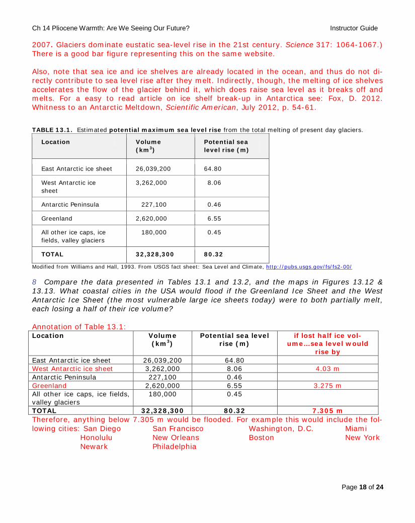
2007. Glaciers dominate eustatic sea-level rise in the 21st century. Science 317: 1064-1067.) There is a good bar figure representing this on the same website. Also, note that sea ice and ice shelves are already located in the ocean, and thus do not di-rectly contribute to sea level rise after they melt. Indirectly, though, the melting of ice shelves accelerates the flow of the glacier behind it, which does raise sea level as it breaks off and melts. For a easy to read article on ice shelf break-up in Antarctica see: Fox, D. 2012. Whitness to an Antarctic Meltdown, Scientific American, July 2012, p. 54-61. TABLE 13.1. Estimated potential maximum sea level rise from the total melting of present day glaciers.

Location Volume (km3)

Potential sea level rise (m)

East Antarctic ice sheet 26,039,200 64.80

West Antarctic ice sheet

3,262,000 8.06

Antarctic Peninsula 227,100 0.46

Greenland 2,620,000 6.55

All other ice caps, ice fields, valley glaciers

180,000 0.45

TOTAL 32,328,300 80.32

Modified from Williams and Hall, 1993. From USGS fact sheet: Sea Level and Climate, http://pubs.usgs.gov/fs/fs2-00/ 8 Compare the data presented in Tables 13.1 and 13.2, and the maps in Figures 13.12 & 13.13. What coastal cities in the USA would flood if the Greenland Ice Sheet and the West Antarctic Ice Sheet (the most vulnerable large ice sheets today) were to both partially melt, each losing a half of their ice volume? Annotation of Table 13.1: Location Volume

(km3) Potential sea level

rise (m) if lost half ice vol-

ume…sea level would rise by

East Antarctic ice sheet 26,039,200 64.80 West Antarctic ice sheet 3,262,000 8.06 4.03 m Antarctic Peninsula 227,100 0.46 Greenland 2,620,000 6.55 3.275 m All other ice caps, ice fields, valley glaciers

180,000 0.45

TOTAL 32,328,300 80.32 7.305 m Therefore, anything below 7.305 m would be flooded. For example this would include the fol-lowing cities: San Diego San Francisco Washington, D.C. Miami

Honolulu New Orleans Boston New York Newark Philadelphia

http://pubs.usgs.gov/fs/fs2-00/�


of 24

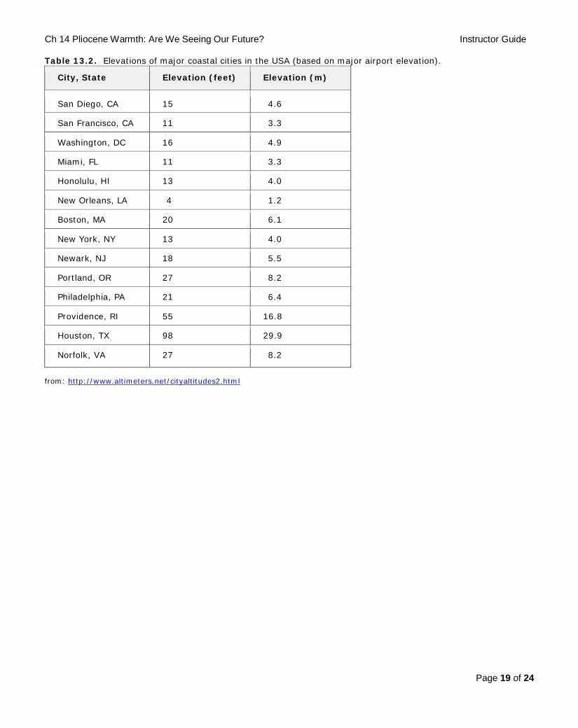
Table 13.2. Elevations of major coastal cities in the USA (based on major airport elevation).

City, State Elevation (feet) Elevation (m)

San Diego, CA 15 4.6

San Francisco, CA 11 3.3

Washington, DC 16 4.9

Miami, FL 11 3.3

Honolulu, HI 13 4.0

New Orleans, LA 4 1.2

Boston, MA 20 6.1

New York, NY 13 4.0

Newark, NJ 18 5.5

Portland, OR 27 8.2

Philadelphia, PA 21 6.4

Providence, RI 55 16.8

Houston, TX 98 29.9

Norfolk, VA 27 8.2

from: http://www.altimeters.net/cityaltitudes2.html

http://www.altimeters.net/cityaltitudes2.html�


of 24

FIGURE 13.12. Series of maps depicting the extent of flooding (red areas) of the southeast USA coastal plain caused by sea level rise: upper left = 1 m, upper right = 2 m, lower left = 4 m, and lower right = 8 m. Courtesy of the National Geophysical Fluid Dynamics Laboratory: http://www.gfdl.noaa.gov/climate-impact-of-quadrupling-co2

http://www.gfdl.noaa.gov/climate-impact-of-quadrupling-co2�


of 24

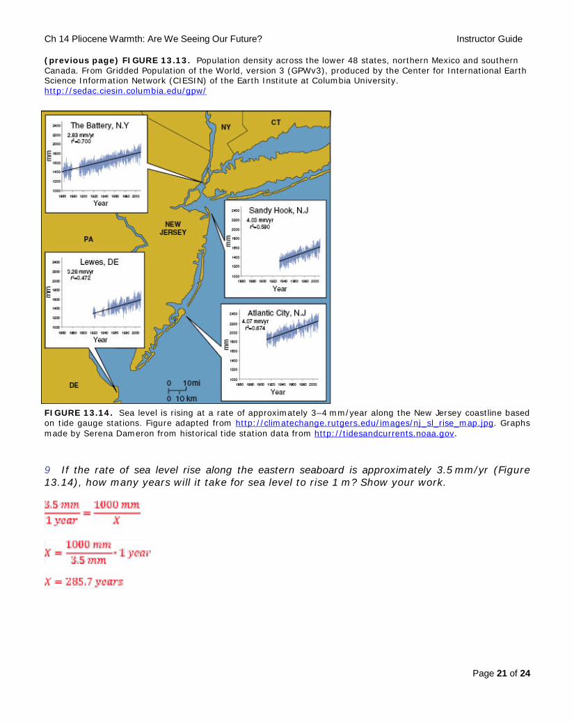
(previous page) FIGURE 13.13. Population density across the lower 48 states, northern Mexico and southern Canada. From Gridded Population of the World, version 3 (GPWv3), produced by the Center for International Earth Science Information Network (CIESIN) of the Earth Institute at Columbia University. http://sedac.ciesin.columbia.edu/gpw/

FIGURE 13.14. Sea level is rising at a rate of approximately 3–4 mm/year along the New Jersey coastline based on tide gauge stations. Figure adapted from http://climatechange.rutgers.edu/images/nj_sl_rise_map.jpg. Graphs made by Serena Dameron from historical tide station data from http://tidesandcurrents.noaa.gov. 9 If the rate of sea level rise along the eastern seaboard is approximately 3.5 mm/yr (Figure 13.14), how many years will it take for sea level to rise 1 m? Show your work.

http://sedac.ciesin.columbia.edu/gpw/�

http://climatechange.rutgers.edu/images/nj_sl_rise_map.jpg�

http://tidesandcurrents.noaa.gov/�


of 24

10 Sea level is rising at a rate of approximately 6 mm/year along the Virginia coastline (Zer-vas, 2009), and approximately 9 mm/year along the periphery of the Mississippi River delta in Louisiana (Miner et al., 2009). The 2007 IPCC Report states that the average global rate of sea level rise for the period of 1950–2000 was approximately 1.8 mm/yr. Speculate about why the rate of sea level rise is so much higher along the eastern and Gulf seaboards of the USA compared to the global average.

This questions aims to have students think about the difference between local changes in sea level and global average (eustatic) changes in sea level. Students may speculate that the land along these coasts is sinking (subsiding, which is cor-rect) there. Others may speculate that rivers are bringing in more water so that it is building up there. This is a good opportunity to determine students’ prior knowledge. 11 Note that sea level is relative to the land surface and, in some places, the land is also subsiding (sinking) in addition to being submerged by the rising global sea level. Speculate about what might cause subsidence in the eastern and Gulf coasts of the USA? Both the eastern and Gulf coasts are passive margins, with large volumes of sediment being transported to, and deposited along the coast. This added weight causes subsidence (sinking) of the coastal zone, which in turn means that the local mean sea level rise is greater along these coasts than the global average. Groundwater, oil, and gas extraction also contribute to land subsidence, especially in the Gulf coast. Along the eastern coast at least, this might also be the result of slow, post-glacial isostatic adjustment of the North American continental crust. Long after the Laurentide Ice Sheet melted the crust beneath it and south of it adjusts. Somewhat like a sea saw, the land be-neath it has been rebounding (rising) as the weight of the ice sheet decreased, while the land south of the ice sheet has been subsiding. III. Summative Assessment

There are several ways the instructor can assess student learning after completion of this ex-ercise. For example, students should be able to answer the following short-answer questions after completing this exercise:

1. Describe the paleogeography, climate (the mean annual temperature, latitudinal tem-perature gradient, ice volume, pCO2), and sea level of the early to mid-Pliocene time (approximately 5–3 Ma).

2. Is the early to mid-Pliocene a good analog for the evolving trends of global warming

today? Why or why not?

3. Describe the evidence (think back to Part 13.1 – δ18O data and lithologic data from ANDRILL 1-B in Antarctica) for orbital influences on climate in the early to mid-Pliocene.

4. What is the PRISM project?

5. What region(s) of the world appear most sensitive to climate forcings? Why?


of 24

6. Challenge: If atmospheric CO2 levels were the same or lower in the early to mid-

Pliocene than today, then how was it that global average temperatures were warmer in the early to mid-Pliocene than today? What lesson does this have for predictions of fu-ture climate?

7. How has sea level changed since the mid-Pliocene? What caused the sea level to change during this time?

8. How does recent regional sea level change along the eastern and Gulf coasts of the US compare to sea level change globally? What drive the differences you describe?

9. Extension: Does the rate sea level rise along the eastern and Gulf coasts warrant con-cern of city planners and local governments in these cities? If not, why not? If so, what actions would you recommend that they take to address the challenge of continued sea level rise?

IV. Supplemental Materials

• For information on the Pliocene Research, Interpretation and Synoptic Mapping (PRISM) project go to: http://geology.er.usgs.gov/eespteam/prism/.

• For very nice interactive maps showing areas potentially impacted by 1 to 3 meter of sea level rise go to the links for “web map visualization tools” at: http://www.geo.arizona.edu/dgesl/research/other/climate_change_and_sea_level/mapping_slr/. Be sure to follow their instructions for optimal visualization and interaction.

• For current data on atmospheric CO2 levels go to the NOAA Earth System Research Laboratory (ESRL) Global Monitoring Division site: http://www.esrl.noaa.gov/gmd/ccgg/.

V. References Ballantyne, A.P., et al., 2010, Significantly warmer Arctic surface temperatures during the

Pliocene indicated by multiple independent proxies. Geology, 38(7), 603–6.

Dowsett, H.J. and Robinson, M.M., 2009, Mid-Pliocene equatorial Pacific sea surface tempera-ture reconstruction: A multi-proxy perspective. Philosophical Transactions of the Royal Soci-ety A, 367, 109–25.

IPCC, 2007, Summary for Policymakers, In Climate Change 2007: The Physical Science Basis. Solomon, S., et al. (eds). Contribution of Working Group I to the Fourth Assessment Report of the Intergovernmental Panel on Climate Change, Cambridge University Press, Cambridge, UK and New York, USA.

Lisiecki, L.E. and Raymo, M.E., 2005, A Pliocene–Pleistocene stack of 57 globally distributed benthic δ18O records. Paleoceanography, 20, doi:10.1029/2004PA001071.

Miner, M.D., et al., 2009, Delta lobe degradation and hurricane impacts governing large-scale coastal behavior, south-central Louisiana. Geo-Marine Letters, 29, 441–53.

Pagani, M., et al., 2009, High Earth-system climate sensitivity determined from Pliocene car-

http://geology.er.usgs.gov/eespteam/prism/�

http://www.geo.arizona.edu/dgesl/research/other/climate_change_and_sea_level/mapping_slr/�

http://www.geo.arizona.edu/dgesl/research/other/climate_change_and_sea_level/mapping_slr/�

http://www.esrl.noaa.gov/gmd/ccgg/�


of 24

bon dioxide concentrations. Nature Geoscience, 3, 27–30, doi:10.1038/ngeo724.

Williams, R.S. and Hall, D.K., 1993, Glaciers, in Chapter on the cryo-sphere. In Atlas of Earth Observations Related to Global Change. Gurney, R.J., et al. (eds), Cambridge University Press, Cambridge, UK, pp. 401–22.

Zervas, C., 2009, Sea level variations of the United States 1854–2006. NOAA Technical Re-port, NOS CO-OPS, US Department of Commerce, National Oceanic and Atmospheric Ad-ministration, National Ocean Service., Silver Spring, MD.

Chapter 13 INSTRUCTOR GUIDE Pliocene Warmth: Are · PDF fileChapter 13 INSTRUCTOR GUIDE....

Documents

Transcript of Chapter 13 INSTRUCTOR GUIDE Pliocene Warmth: Are · PDF fileChapter 13 INSTRUCTOR GUIDE....