BDA 30703

INTRODUCTION

to

INSTRUMENTATION and MEASUREMENT

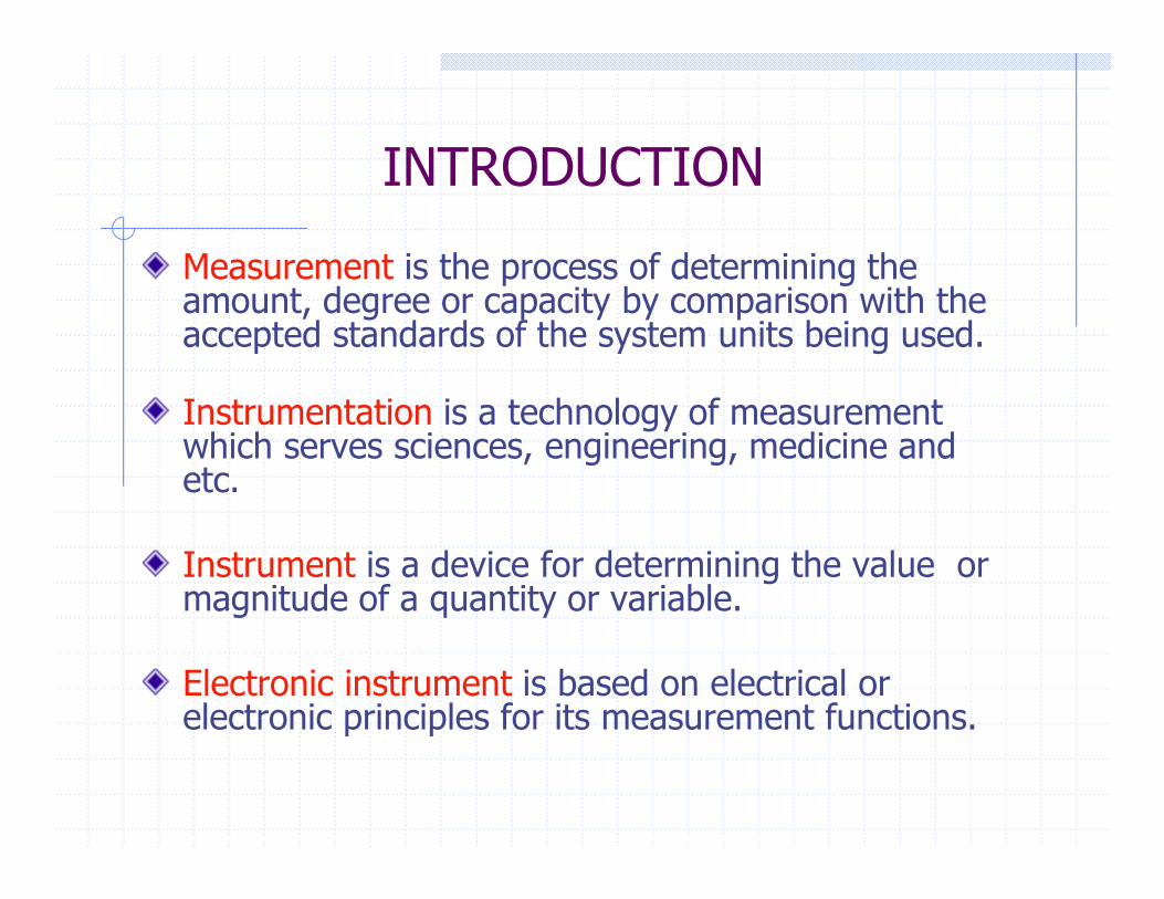
INTRODUCTION

Measurement is the process of determining the amount, degree or capacity by comparison with the accepted standards of the system units being used.

Instrumentation is a technology of measurement which serves sciences, engineering, medicine and etc.

Instrument is a device for determining the value or magnitude of a quantity or variable.

Electronic instrument is based on electrical or electronic principles for its measurement functions.

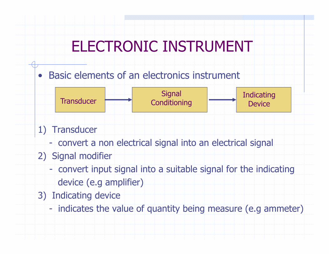
ELECTRONIC INSTRUMENT

1) Transducer

- convert a non electrical signal into an electrical signal

2) Signal modifier

- convert input signal into a suitable signal for the indicating

device (e.g amplifier)

3) Indicating device

- indicates the value of quantity being measure (e.g ammeter)

TransducerSignal

ConditioningIndicating

Device

• Basic elements of an electronics instrument

Transducer/Sensors

An analogue instrument gives an output that varies continuously as the quantity being measured; e.g. Deflection-type of pressure gauge

5

Analogue Instruments

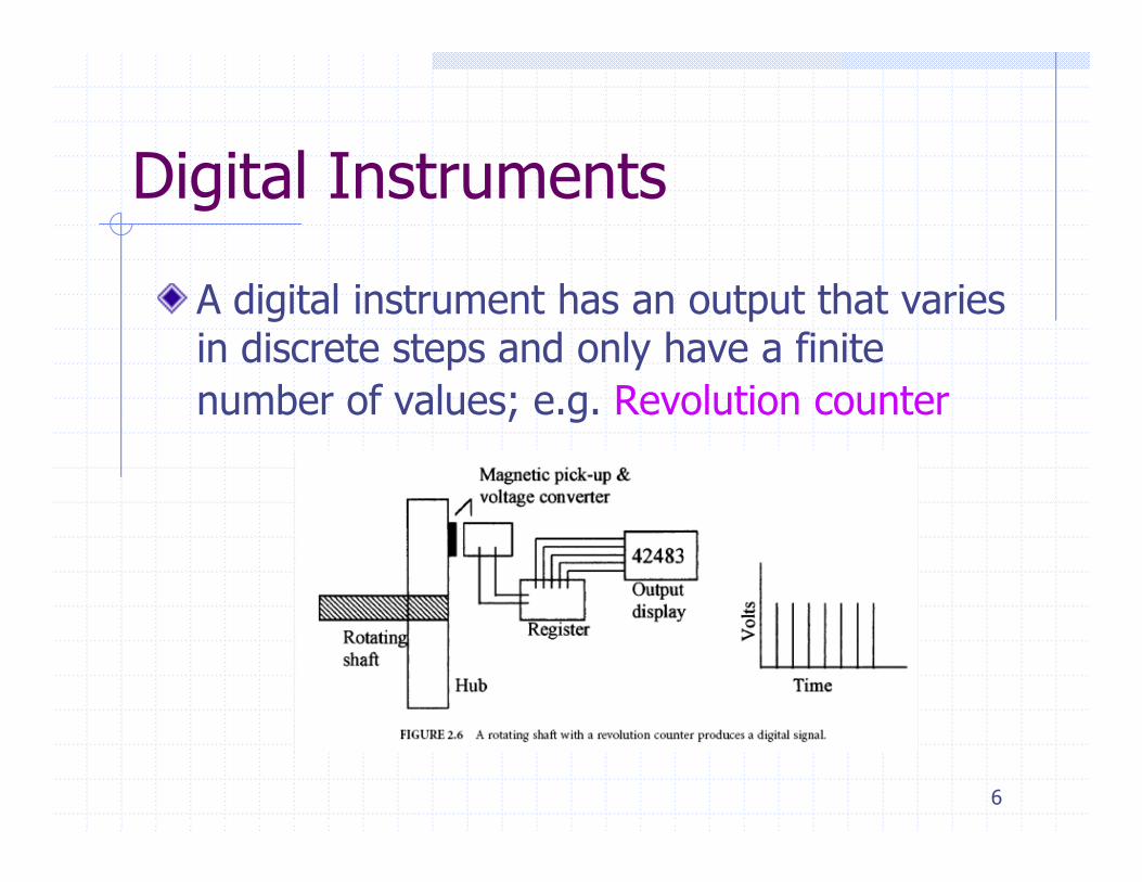
A digital instrument has an output that varies in discrete steps and only have a finite

number of values; e.g. Revolution counter

6

Digital Instruments

Sensor Outputs

FUNCTIONS

The 3 basic functions of instrumentation :-

Indicating – visualize the process/operation

Recording – observe and save the measurement reading

Controlling – to control measurement and process

PERFORMANCE CHARACTERISTICS

Performance Characteristics - characteristics that show the performance of an instrument.

Eg: accuracy, precision, resolution, sensitivity.

Allows users to select the most suitable instrument for a specific measuring jobs.

Two basic characteristics :

Static

Dynamic

Static Characteristic of Instruments

Accuracy – the degree of exactness of measurement compared to the expected value.

Resolution – the smallest change in a measurement variable to which an instrument will respond.

Precision – a measure of consistency or repeatability of measurement.

Error – the deviation of the true value from the desired value.

Sensitivity – ratio of change in the output of instrument to a change of input or measured variable.

Tolerance - maximum deviation of a component from some specified value.

Range or span - minimum and maximum values of a quantity that the instrument is designed to measure.

Linearity - output reading of an instrument that is linearly proportional to the quantity being measured

Measurement Sensitivity -measure of the change in instrument output that occurs when the quantity being measured changes by a given amount.

Threshold – minimum scale of measurement.

Sensitivity to disturbance – measurement magnitude due to disturbance (zero drfit & sensitivity drift).

Zero drift is the measurement reading when no input is given.

Sensitivity drift is the measurement sensitivity difference when the ambient varies.

Hysteresis, Dead space

11

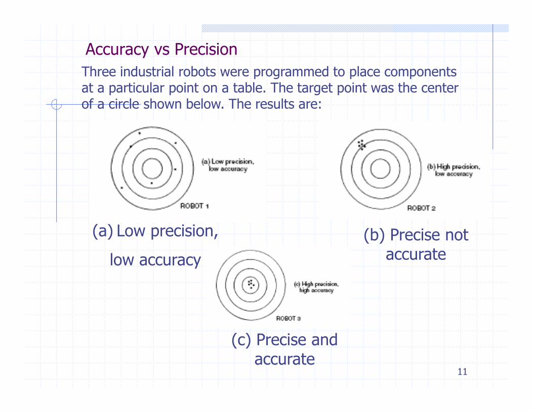
Accuracy vs Precision

(a) Low precision,

low accuracy

(b) Precise not accurate

(c) Precise and accurate

Three industrial robots were programmed to place componentsat a particular point on a table. The target point was the centerof a circle shown below. The results are:

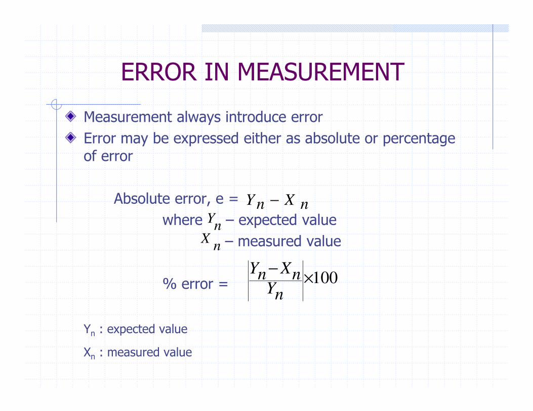
ERROR IN MEASUREMENT

Measurement always introduce error

Error may be expressed either as absolute or percentage of error

Absolute error, e =

where – expected value

– measured value

% error =

Yn : expected value

Xn : measured value

100×−

nY

nX

nY

nXnY −

nX

nY

ERROR IN MEASUREMENT

Relative accuracy,

% Accuracy, a = 100% - % error

=

n

nn

Y

XYA

−−=1

100×A

Example;

Given expected voltage value across a resistor is 80V but the measured voltage is 79V. Calculate,

i. The absolute error

ii. The % of error

iii. The relative accuracy

iv. The % of accuracy

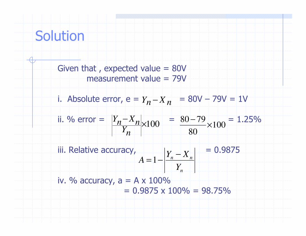
Solution

Given that , expected value = 80Vmeasurement value = 79V

i. Absolute error, e = = 80V – 79V = 1V

ii. % error = = = 1.25%

iii. Relative accuracy, = 0.9875

iv. % accuracy, a = A x 100% = 0.9875 x 100% = 98.75%

nXnY −

10080

7980×

−100×

−

nY

nX

nY

n

nn

Y

XYA

−−=1

STATIC CHARACTERISTICS ~ Measurement Sensitivity

Example 1

The following pressure values, y (mmHg) of a Piezoelectric Device were measured

at a range of temperatures, x (oC). Determine the measurement sensitivity of the

instrument

in mmHg /°C.

Soluition;

For a change in temperature of 5 oC , the change in pressure is 13.1 mmHg. Hence

the measurement sensitivity ;

= 13.1 mmHg/5 oC

= 2.62 mmHg/ oC

STATIC CHARACTERISTICS ~ Sensitivity to disturbance

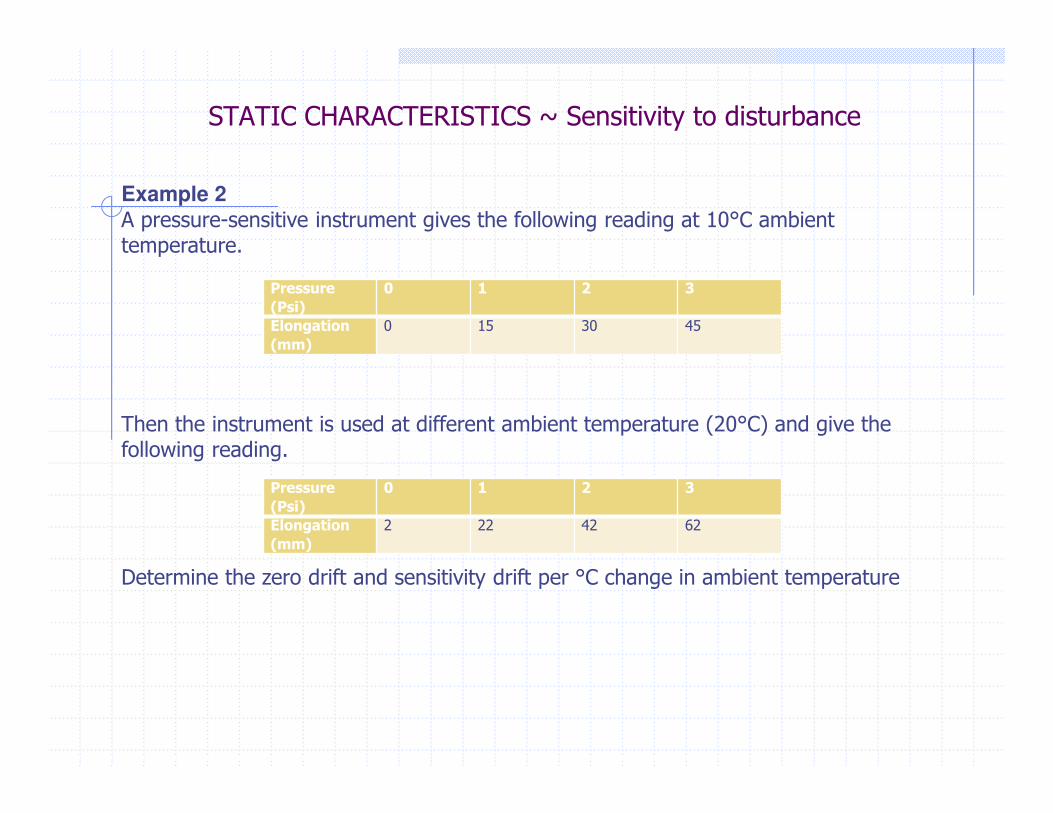
Example 2

A pressure-sensitive instrument gives the following reading at 10°C ambient temperature.

Then the instrument is used at different ambient temperature (20°C) and give the following reading.

Determine the zero drift and sensitivity drift per °C change in ambient temperature

Pressure

(Psi)

0 1 2 3

Elongation

(mm)

0 15 30 45

Pressure

(Psi)

0 1 2 3

Elongation

(mm)

2 22 42 62

STATIC CHARACTERISTICS ~ Sensitivity to disturbance

Example 2 (Solution)

At 10°C, the elongation/pressure is a straight line. Measurement sensitivity is 15 mm/psi.At 20°C, the elongation/pressure is a straight line. Measurement sensitivity is 20 mm/psi.

Zero drift = 2 mm (no-pressure elongation)Sensitivity drift = Difference of Measurement Sensitivity = 20 mm/psi - 15 mm/psi

= 5 mm/psiZero drift/°C = 2 mm / 10°C = 0.2 mm/°C

Measurement Sensitivity/°C =5 mm/psi/ 10°C = 0.5 mm/psi °C

TYPES OF STATIC ERROR

Types of error in measurement:

1) Gross error/human error

2) Systematic Error

3) Random Error

1) Gross Error

- caused by human mistakes in reading/using instruments

- cannot eliminate but can minimize

TYPES OF STATIC ERROR (cont)

2) Systematic Error

- due to shortcomings of the instrument (such as

defective or worn parts)

- 3 types of systematic error :-

(i) Instrumental error

(ii) Environmental error

(iii) Observational error, e.g; parallax error

TYPES OF STATIC ERROR (cont)

3) Random error

- due to unknown causes, occur when all systematic

error has accounted.

- E.g. +ve & -ve errors in approximately equal numbers.

for a series of measurements made of the same quantity

- accumulation of small effect, require at high degree

of accuracy.

- caused by unpredictable variations in the measurement

system.

- can be avoided by;

(a) increasing number of reading

(b) use statistical means to obtain best approximation of true value

Measurement Systems with Electrical Signals

• displacement,• linear velocity,• Angular• velocity,• acceleration,• force,• pressure,• temperature,• heat flux,• humidity, • fluid flow rate,• light intensity,• Chemical

Characteristic• chemical

composition.

• Amplification

• Attenuation

• Filtering (highpass,

Iowpass, bandpass, or

bandstop)

• Differentiation

• Integration

• Linearization

• Converting a resistance to

a voltage signal

• Converting a current signal

to a voltage signal

• gage,• cell,• pickup,• Transmitter

Converts physical changes to electrical pulses

• Display• Screen• Metering• Scales• Systems

More than one signal-conditioning function, such as amplification and filtering, can

be performed on a signal.

Operational Amplifier Applications

Audio amplifiers

Speakers and microphone circuits in cell phones, computers, mpg players, boom boxes, etc.

Instrumentation amplifiers

Biomedical systems including heart monitors and oxygen sensors.

Power amplifiers

Analog computers

Combination of integrators, differentiators, summing amplifiers, and multipliers

What is an Op-Amp? – The

Surface• An Operational Amplifier (Op-Amp) is an integrated circuit that

uses external voltage to amplify the input through a very high

gain.

• We recognize an Op-Amp as a mass-produced component

found in countless electronics.

What an Op-Amp looks

like to a lay-person

What an Op-Amp looks

like to an engineer

Ideal Operational Amplifier

Operational amplifier (Op-amp) is made of many transistors,

diodes, resistors and capacitors in integrated circuit technology.

Ideal op-amp is characterized by:

Infinite input impedance

Infinite gain for differential input

Zero output impedance

Infinite frequency bandwidth

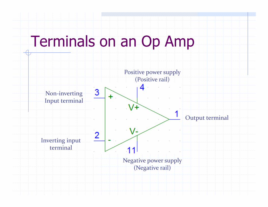
Terminals on an Op Amp

Non-inverting Input terminal

Inverting inputterminal

Output terminal

Positive power supply (Positive rail)

Negative power supply (Negative rail)

Winter 2012

UCSD: Physics 121; 2012

27

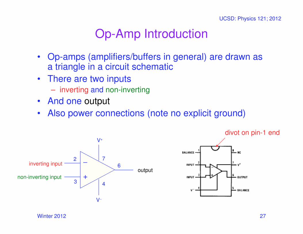
Op-Amp Introduction

• Op-amps (amplifiers/buffers in general) are drawn as a triangle in a circuit schematic

• There are two inputs– inverting and non-inverting

• And one output

• Also power connections (note no explicit ground)

−

+

2

3 4

7

6

divot on pin-1 end

inverting input

non-inverting input

V+

V−

output

Winter 2012

UCSD: Physics 121; 2012

28

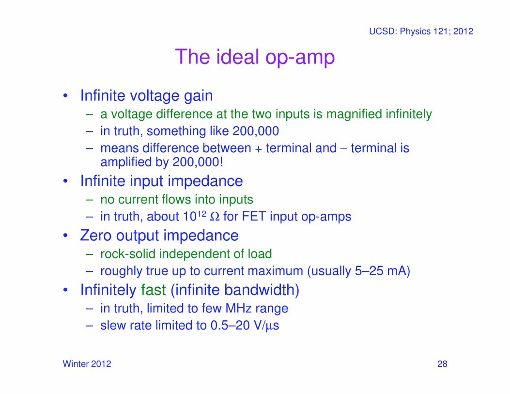
The ideal op-amp

• Infinite voltage gain– a voltage difference at the two inputs is magnified infinitely

– in truth, something like 200,000

– means difference between + terminal and − terminal is amplified by 200,000!

• Infinite input impedance– no current flows into inputs

– in truth, about 1012 Ω for FET input op-amps

• Zero output impedance– rock-solid independent of load

– roughly true up to current maximum (usually 5–25 mA)

• Infinitely fast (infinite bandwidth)– in truth, limited to few MHz range

– slew rate limited to 0.5–20 V/µs

Winter 2012

UCSD: Physics 121; 2012

29

Op-amp without feedback

• The internal op-amp formula is:

Vout = gain×(V+ − V−)

• So if V+ is greater than V−, the output goes positive

• If V− is greater than V+, the output goes negative

• A gain of 200,000 makes this device (as illustrated

here) practically useless

−

+

V−

V+

Vout

Winter 2012

UCSD: Physics 121; 2012

30

Infinite Gain in negative feedback

• Infinite gain would be useless except in the self-

regulated negative feedback regime

– negative feedback seems bad, and positive good—but in electronics positive feedback means runaway or oscillation, and negative feedback leads to stability

• Imagine hooking the output to the inverting terminal:

• If the output is less than Vin, it shoots positive

• If the output is greater than Vin, it shoots negative

– result is that output quickly forces itself to be exactly Vin

−

+Vin

negative feedback loop

Winter 2012

UCSD: Physics 121; 2012

31

Op-Amp “Golden Rules”

• When an op-amp is configured in any negative-

feedback arrangement, it will obey the following two

rules:

– The inputs to the op-amp draw or source no current (true whether negative feedback or not)

– The op-amp output will do whatever it can (within its limitations) to make the voltage difference between the two inputs zero

UCSD: Physics 121; 2012

Inverting Op-Amp

• Applying the rules: − terminal at “virtual ground”

– so current through R1 is If = Vin/R1

• Current does not flow into op-amp (one of our rules)

– so the current through R1 must go through R2

– voltage drop across R2 is then IfR2 = Vin×(R2/R1)

• So Vout = 0 − Vin×(R2/R1) = −Vin×(R2/R1);

Vout = −−−−Vin××××(R2/R1)

• Thus we amplify Vin by factor −R2/R1

– negative sign earns title “inverting” amplifier

−

+

Vin

Vout

R1

R2

UCSD: Physics 121; 2012

33

Inverting Op-Amp example

−

+

Vin

Vout

R1

R2

If Vin is 0.2V, R1 = 10 kΩ and R2 = 150 kΩ , calculate the output voltage Vout

and the current on R1.

Solution.This is an inverting Op-Amp, Vout = -Vin x R2/R1 = -0.2 x 150/10 = - 3 V.

Current on R1,I1 = Vin/R1 = 0.2 V /(10 x 1000 Ω) = 0.00002 A = 20 µA.

Non-inverting Op-Amp

• Now neg. terminal held at Vin

– so current through R1 is If = Vin/R1 (to left, into ground)

• This current cannot come from op-amp input

– so comes through R2 (delivered from op-amp output)

– voltage drop across R2 is IfR2 = Vin×(R2/R1)

– so that output is higher than neg. input terminal by Vin×(R2/R1)

– Vout = Vin + Vin×(R2/R1) = Vin×(1 + R2/R1)

Vout = Vin××××(1+ R2/R1)

– thus gain is (1 + R2/R1), and is positive

−

+Vin

Vout

R1

R2

Non-inverting Op-Amp example.

−

+Vin

Vout

R1

R2

If Vin is 0.2V, R1 = 10 kΩ and R2 = 150 kΩ , calculate the output voltage Vout

and the current on R1.

Solution.This is an inverting Op-Amp, Vout = Vin x (1+ R2/R1 = 0.2 x (1+150/10) = 3.2 V.

Current on R1,I1 = Vin/R1 = 0.2 V /(10 x 1000 Ω) = 0.00002 A = 20 µA.

Applications of Op-Amps• Electrocardiogram (EKG) Amplification

– Need to measure difference in voltage from lead 1 and lead 2

– 60 Hz interference from electrical equipment

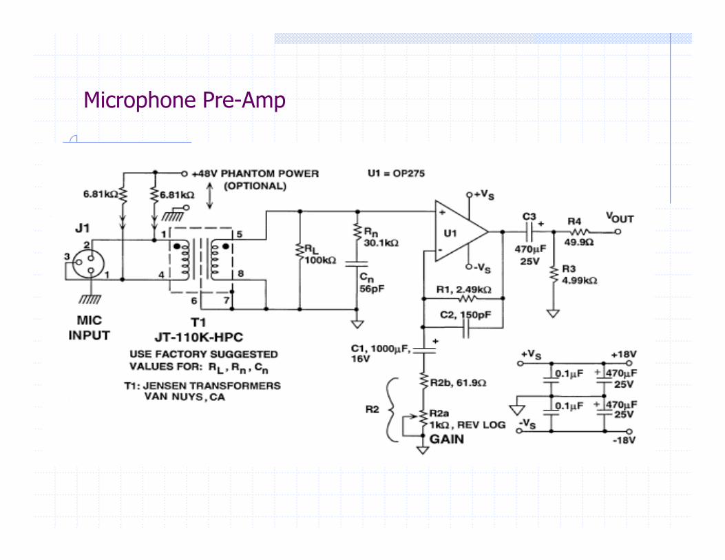
Microphone Pre-Amp

Applications of Op-Amps• Piezoelectric Transducer

– Used to measure force, pressure, acceleration

– Piezoelectric crystal generates an electric

charge in response to deformation

• Use Charge Amplifier

– Just an integrator op-amp circuit

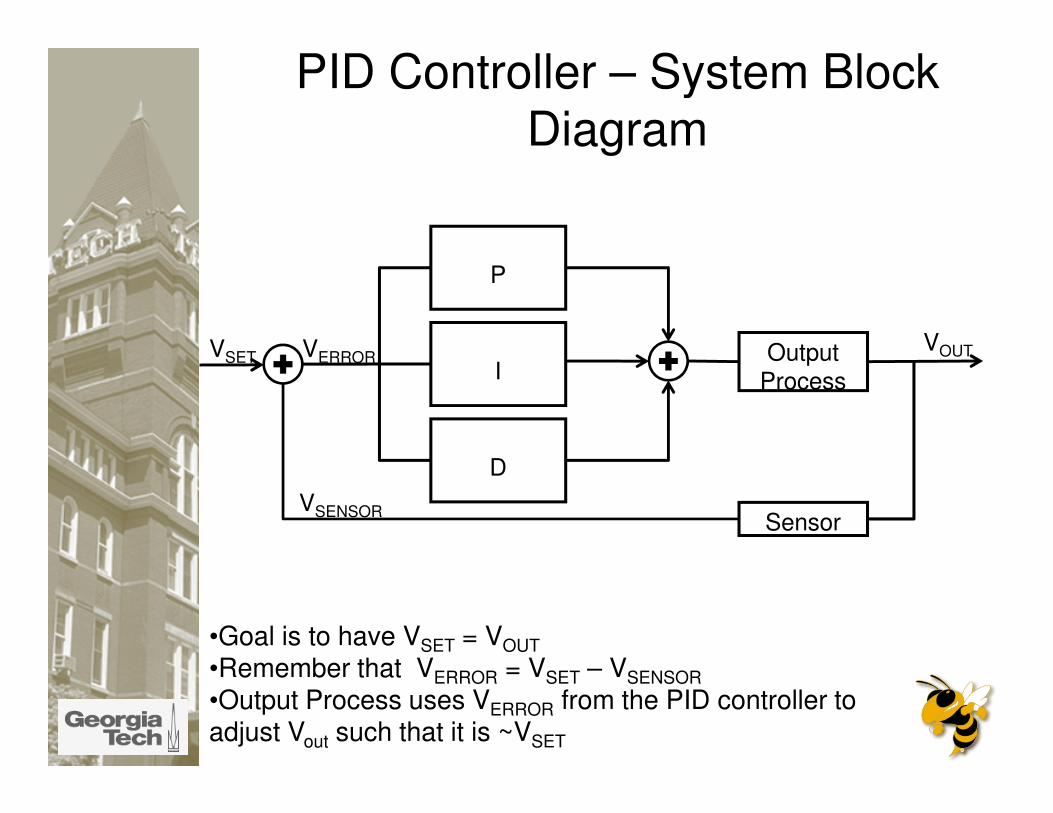
•Goal is to have VSET = VOUT

•Remember that VERROR = VSET – VSENSOR

•Output Process uses VERROR from the PID controller to adjust Vout such that it is ~VSET

P

I

D

Output

Process

Sensor

VERRORVSETVOUT

VSENSOR

PID Controller – System Block

Diagram

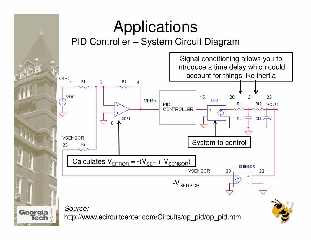
ApplicationsPID Controller – System Circuit Diagram

Source:

http://www.ecircuitcenter.com/Circuits/op_pid/op_pid.htm

Calculates VERROR = -(VSET + VSENSOR)

Signal conditioning allows you to

introduce a time delay which could

account for things like inertia

System to control

-VSENSOR

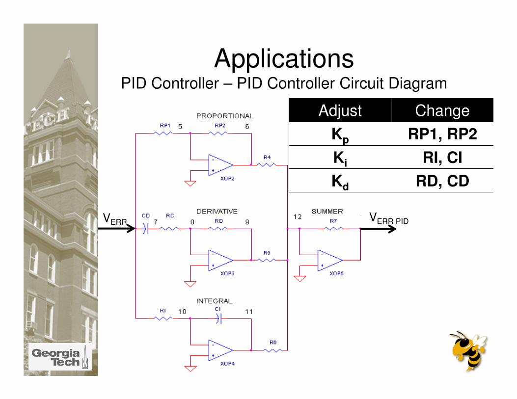
ApplicationsPID Controller – PID Controller Circuit Diagram

VERR

Adjust Change

Kp RP1, RP2

Ki RI, CI

Kd RD, CD

VERR PID

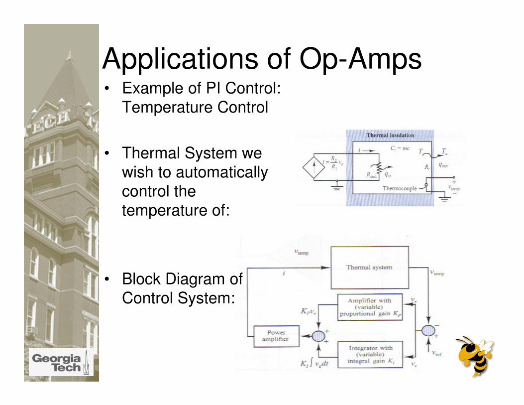
Applications of Op-Amps• Example of PI Control:

Temperature Control

• Thermal System we

wish to automatically

control the

temperature of:

• Block Diagram of

Control System:

Applications of Op-Amps

• Voltage

Error

Circuit:

• Proportion

al-Integral

(PI)

Control

Circuit:

• Example of PI Control: Temperature Control

741 Op-Amp in the Circuit

741 Op-Amp Schematic

differential amplifier high-gain amplifier

voltage

level

shifteroutput

stage

current mirror

current mirror current mirror

Revisit/Recap

1. Parallel/Series spring & damper.2. 2nd order Nyquist plots