CFD Modeling Coolingtower-final2

SRNL-STI-2009-00137

Key Words:

Cooling Tower, Computational Fluid Dynamics, Heat Transfer

Retention: Permanent

CFD MODELING AND ANALYSIS FOR A-AREA AND H-AREA COOLING TOWERS

S. Y. Lee, A. J. Garrett, and J. S. Bollinger

AUGUST 2009

Savannah River National Laboratory Savannah River Nuclear Solutions Aiken, SC 29808

Prepared for the U.S. Department of Energy Under Contract Number DE-AC09-08SR22470

SRNL-STI-2009-00137

DISCLAIMER

This work was prepared under an agreement with and funded by the U.S. Government. Neither the U. S. Government or its employees, nor any of its contractors, subcontractors or their employees, makes any express or implied: 1. warranty or assumes any legal liability for the accuracy, completeness, or for the use or results of such use of any information, product, or process disclosed; or 2. representation that such use or results of such use would not infringe privately owned rights; or 3. endorsement or recommendation of any specifically identified commercial product, process, or service. Any views and opinions of authors expressed in this work do not necessarily state or reflect those of the United States Government, or its contractors, or subcontractors.

Printed in the United States of America

Prepared for

U.S. Department of Energy

SRNL-STI-2009-00137

Key Words:

Cooling Tower, Computational Fluid Dynamics, Heat Transfer

Retention: Permanent

CFD MODELING AND ANALYSIS FOR A-AREA AND H-AREA COOLING TOWERS

S. Y. Lee, A. J. Garrett, and J. S. Bollinger

AUGUST 2009

Savannah River National Laboratory Savannah River Nuclear Solutions Savannah River Site Aiken, SC 29808

Prepared for the U.S. Department of Energy Under Contract Number DE-AC09-08SR22470

SRNL-STI-2009-00137

- iii -

TABLE OF CONTENTS

LIST OF FIGURES ............................................................................................................... iv

LIST OF TABLES ................................................................................................................. vi

LIST OF ACRONYMS ......................................................................................................... vi

1.0 EXECUTIVE SUMMARY .............................................................................................. 1

2.0 INTRODUCTION............................................................................................................. 2

3.0 MODELING APPROACH AND SOLUTION METHOD ........................................... 6

4.0 MODEL BENCHMARKING........................................................................................ 15

4.1 Model benchmarking for Basic Physical Behaviors................................................. 15

4.2 Integral Benchmarking Results for A-area............................................................... 18

4.3 Integral Benchmarking Results for H-area............................................................... 34

5.0 RESULTS AND DISCUSSIONS................................................................................... 49

6.0 CONCLUSIONS AND SUMMARY ............................................................................. 60

7.0 REFERENCES................................................................................................................ 61

SRNL-STI-2009-00137

- iv -

LIST OF FIGURES

Figure 1. Geometry and dimensions for each of the four cells in A-area Mechanical Draft

Cooling Tower (MDCT) .........................................................................................3 Figure 2. Geometry and dimensions for each of the four cells in H-area Mechanical Draft

Cooling Tower (MDCT) .........................................................................................4 Figure 3. Top view showing cell boundary of H-area tower ...................................................5 Figure 5. Mass, momentum, and heat transfer between the continuous gas phase and

discrete water droplet ............................................................................................6 Figure 6. Solution methods for single-phase mixture modeling approach. ..........................13 Figure 8. Comparison of the pressure drops across the drift eliminator with the literature

data (77% porosity). ............................................................................................16 Figure 9. Benchmarking results of non-dimensional horizontal air velocity along the line A-A’

on the plane of y=2H distance from the air inlet plane at Re = 7,100 inlet flow (inlet air velocity, U = 10.371 m/sec) ...................................................................17

Figure 10. Comparison of the predicted droplet cooling with the test data for free-falling water droplet in still air [10]..................................................................................18

Figure 11. Cross-section view of the compartment cell instrumented for the performance measurement for A-area cooling tower. ..............................................................19

Figure 12. Possible range of droplets sizes for various upward flow air velocities ..............21 Figure 13. Comparison of air temperature at shroud exit for Fast1 test conditions .............23 Figure 14. Comparison of air humidity at shroud exit for Fast1 test conditions ...................24 Figure 15. Air flow patterns for the vertical mid-plane crossing the instrumented cell of the

cooling tower for Fast1 case, showing that red-color vector indicates about 9 m/sec air. .............................................................................................................24

Figure 16. Air temperature distributions for the vertical mid-plane crossing the instrumented cell of the cooling tower for Fast1 case, showing that red-color zone indicates about 26oC...........................................................................................................25

Figure 17. Air mass fractions for the vertical mid-plane crossing the instrumented cell of the cooling tower for Fast1 case, showing that red-color zone indicates about 2.1% mass fraction. ......................................................................................................25

Figure 18. Comparison of air velocity distributions between the models with and without flow obstructions at the horizontal plane 4 ft above the ground surface for Fast1 case.....................................................................................................................26

Figure 19. Comparison of vapor mass fraction distributions between the models with and without shed at the mid-plane of 2nd cell for Fast1 case......................................26

Figure 20. Temperature distributions for water droplets under Fast1 case..........................27 Figure 21. Temperature distributions at the exit of the cooling fan shroud under the no fan

conditions of Nofan5............................................................................................28 Figure 22. Humidity distributions at the exit of the cooling fan shroud under the no fan

conditions of Nofan5............................................................................................28 Figure 23. Variation of air exit temperature for different air mass flow rates driven by fan and

wind .....................................................................................................................29 Figure 24. Variation of water exit temperature for different air mass flow rates driven by fan

and wind ..............................................................................................................29 Figure 25. Evaporative cooling performance of A-Area cooling tower for different air

flowrates ..............................................................................................................30 Figure 26. Comparison of the model predictions with the test results for air exit temperature.

............................................................................................................................30

SRNL-STI-2009-00137

- v -

Figure 27. Comparison of the model predictions with test results for vapor mass fractions at shroud exit. ..........................................................................................................31

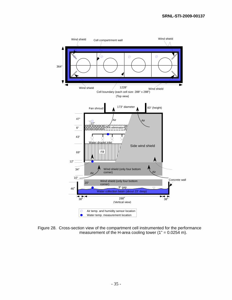
Figure 28. Cross-section view of the compartment cell instrumented for the performance measurement for H-area cooling tower (1” = 0.0254 m). ....................................35

Figure 29. Flow patterns at the plane crossing the vertical center of the 3rd cell under low-speed wind in H-area cooling tower ....................................................................37

Figure 30. Temperature distributions at the plane crossing the vertical center of the 3rd cell under low-speed wind in H-area cooling tower....................................................37

Figure 31. Vapor mass fraction distributions at the plane crossing the vertical center of the 3rd cell under low-speed wind in H-area cooling tower ........................................38

Figure 32. Flow patterns at the plane crossing the vertical center of the 2nd cell under high-speed wind in H-area cooling tower ....................................................................38

Figure 33. Air temperature distributions at the plane crossing the vertical center of the 2nd cell under high-speed wind in H-area cooling tower............................................39

Figure 34. Vapor mass fraction distributions at the plane crossing the vertical center of the 2nd cell under high-speed wind in H-area cooling tower ......................................39

Figure 35. Comparison of flow patterns between fan-on and fan-off cells in H-area cooling tower....................................................................................................................40

Figure 36. Comparison of air temperature distributions between fan-on and fan-off cells at the plane crossing the vertical center of the cell in H-area cooling tower............41

Figure 37. Comparison of vapor mass fractions between fan-on and fan-off cells at the plane crossing the vertical center of the cell in H-area cooling tower..................42

Figure 38. Comparison of flow patterns between high and low wind speeds for H-area cooling tower under the same color scale system...............................................43

Figure 39. Comparison of cell temperature distributions between high and low wind speeds for H-area cooling tower ......................................................................................44

Figure 40. Temperature distributions for water droplets for Aug28 case under H-Area cooling tower .......................................................................................................45

Figure 41. Comparison of predictions with measured air temperatures at exit of H-area cooling tower .......................................................................................................46

Figure 42. Comparison of predictions with measured vapor mass fractions at exit of H-area cooling tower .......................................................................................................46

Figure 43. Comparison of the modeling predictions with the measured air exit temperatures for A-Area and H-Area cooling towers.................................................................50

Figure 44. Comparison of the modeling predictions with the measured vapor mass fractions at exit for A-Area and H-Area cooling towers ......................................................50

Figure 45. Nondimensional velocities at shroud exit as function of wind direction for three different wind speeds in A-Area tower.................................................................51

Figure 46. Nondimensional velocities at shroud exit as function of wind direction for three different wind speeds in H-Area tower.................................................................55

Figure 47. Comparison of the modeling predictions with the measured air exit temperatures for A-Area and H-Area cooling towers under cooling fan-off condition................59

SRNL-STI-2009-00137

- vi -

LIST OF TABLES Table 1. Test conditions and results for the A-Area MDCT..................................................20 Table 2. Comparison of wind velocity predictions around the cooling tower with test data

under the Fast1 conditions .....................................................................................22 Table 3. Comparison of water temperature predictions with test data at 28-in above the

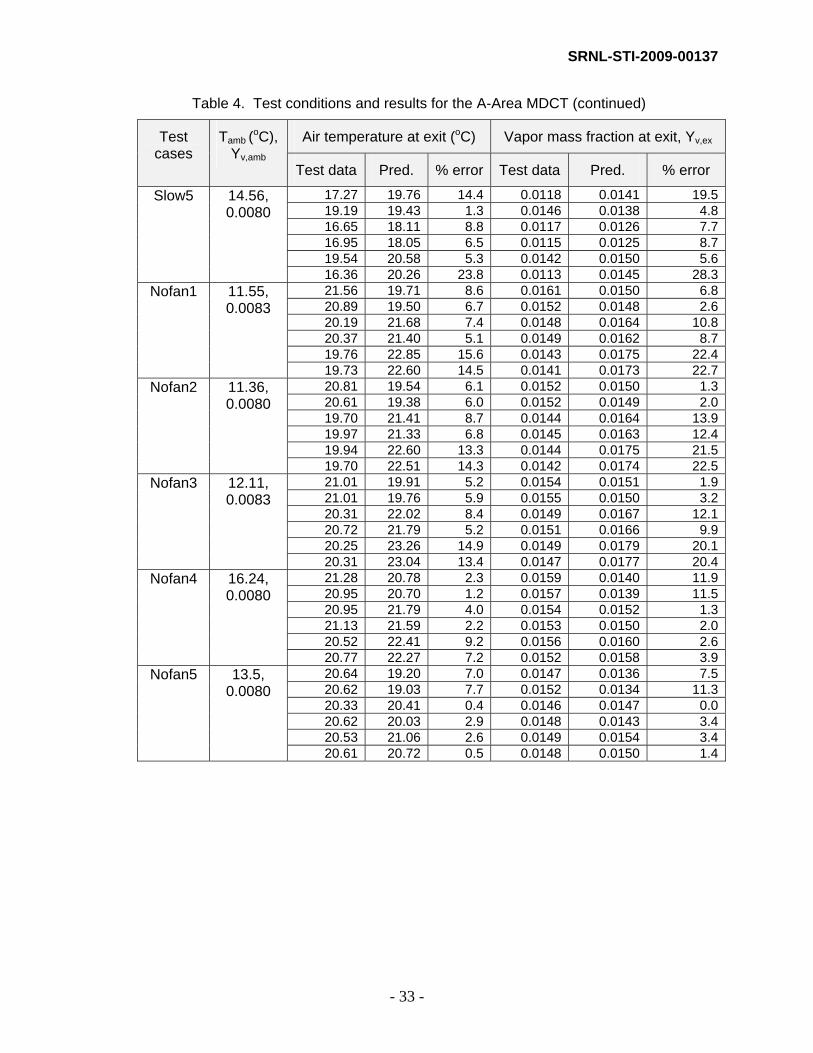
water basin surface under Fast1 operating conditions...........................................27 Table 4. Test conditions and results for the A-Area MDCT..................................................32 Table 4. Test conditions and results for the A-Area MDCT (continued)...............................33 Table 5. Ambient conditions and measurement results for the H-Area MDCT ....................36 Table 6. Comparison of air exit temperatures between the test results and the modeling

predictions for the H-Area MDCT ...........................................................................47 Table 7. Comparison of vapor mass fractions at exit between the test results and the

modeling predictions for the H-Area MDCT ...........................................................48 Table 8. Parametric results for 2 m/sec wind speed with various wind directions under A-

Area cooling tower..................................................................................................52 Table 9. Parametric results for 4 m/sec wind speed with various wind directions under A-

Area cooling tower..................................................................................................53 Table 10. Parametric results for 8 m/sec wind speed with various wind directions under A-

Area cooling tower..................................................................................................54 Table 11. Parametric results for 2 m/sec wind speed with various wind directions under H-



Area cooling tower..................................................................................................58

SRNL-STI-2009-00137

- vii -

LIST OF ACRONYMS °C Degree Centigrade (or Celsius) Cv Vapor mass concentration per unit volume Cvp Vapor mass concentration per unit volume at droplet surface C1ε Constant for turbulent dissipation rate equation (= 1.44) C2ε Constant for turbulent dissipation rate equation (= 1.92) Cµ Constant for turbulent viscosity (= 0.09) d Diameter (m) Dv Vapor diffusion coefficient (m2/sec) F External body force that arises from interaction with the dispersed phase in

porous-media h Air inlet height (m), heat transfer coefficient (W/m2-K) hsm Sensible specific enthalpy of the gas mixture (J/kg) hsv Sensible specific enthalpy of the vapor species (J/kg) H Room height (m) hr Hour

vJv

Diffusion flux of vapor species k Thermal conductivity (W/m-K) kg Kilogram kh,eff Effective thermal conductivity (W/m-K) km Mass transfer coefficient based on driving force of mass density to give mass

flux (m/sec) L Length (m) or latent heat (cal/gm) MH2O Water molecular weight m Meter mm millimeter min Minute R* universal gas constant (= 8.3144x107 erg/(mol-K)) Sv Mass addition to the continuous air phase due to the evaporation of the water

droplets t Air outlet height (m) or time (sec) Tamb Ambient air temperature (oC) Tp Water droplet temperature (oC) Twi Water temperature at water distribution deck (oC) Uo Wind speed (m/sec) v Local air velocity (m/sec) vex Velocity at exit of fan shroud (m/sec) W Room width (m) x, y, z Three coordinate system for the computational domain as shown Fig. 1 Xv Local mole fraction of vapor species Yv,amb Vapor mass fraction of the mixture at ambient condition Yv,ex Vapor mass fraction of the mixture at shroud exit Yv Vapor mass fraction of the mixture at local point θo Wind direction w.r.t. plant north k Turbulence kinetic energy (m2/sec2) g Specific humidity (air mass present in the air per unit air mass) ε Turbulence energy dissipation rate (m2/sec3) ρ Density of the Air and vapor mixture (kg/m3) φ Relative humidity

SRNL-STI-2009-00137

- viii -

φm Vapor mass flux µ Dynamic viscosity (kg/m-sec) µt Turbulent dynamic viscosity (kg/m-sec) σk Turbulent Prandtl number for turbulent kinetic energy (=1.0 for fully

turbulent flow) σε Turbulent Prandtl number for turbulent energy dissipation rate (=1.3 for

fully turbulent flow) CFD Computational Fluid Dynamics DOE U.S. Department of Energy MDCT Mechanical Draft Cooling Tower Nu Nusselt number (=

khd )

Pr Prandtl number (= ρCpµ/k)

Sh Sherwood number (v

pm

Ddk

= )

Pa Pascal (N/m2) PN Plant north Re Reynolds number (dρv/µ) RH Relative humidity RSM Reynolds Stress Model s or sec Second SRNL Savannah River National Laboratory SRS Savannah River Site WSRC Washington Savannah River Company

SRNL-STI-2009-00137

- 1 -

1.0 EXECUTIVE SUMMARY Industrial processes use mechanical draft cooling towers (MDCT’s) to dissipate waste heat by transferring heat from water to air via evaporative cooling, which causes air humidification. The Savannah River Site (SRS) has a MDCT consisting of four independent compartments called cells. Each cell has its own fan to help maximize heat transfer between ambient air and circulated water. The primary objective of the work is to conduct a parametric study for cooling tower performance under different fan speeds and ambient air conditions.

The Savannah River National Laboratory (SRNL) developed a computational fluid dynamics (CFD) model to achieve the objective. The model uses three-dimensional momentum, energy, continuity equations, air-vapor species balance equation, and two-equation turbulence as the basic governing equations. It was assumed that vapor phase is always transported by the continuous air phase with no slip velocity. In this case, water droplet component was considered as discrete phase for the interfacial heat and mass transfer via Lagrangian approach. Thus, the air-vapor mixture model with discrete water droplet phase is used for the analysis.

A series of the modeling calculations was performed to investigate the impact of ambient and operating conditions on the thermal performance of the cooling tower when fans were operating and when they were turned off. The model was benchmarked against the literature data and the SRS test results for key parameters such as air temperature and humidity at the tower exit and water temperature for given ambient conditions. Detailed modeling and test results will be presented here.

SRNL-STI-2009-00137

- 2 -

2.0 INTRODUCTION Mechanical draft cooling towers are designed to cool process water via sensible and latent heat transfer to air. Heat and mass transfer take place simultaneously. Heat is transferred as sensible heat due to the temperature difference between liquid and gas phases, and as the latent heat of the water as it evaporates. Mass of water vapor is transferred due to the difference between the vapor pressure at the air-liquid interface and the partial pressure of water vapor in the bulk of the air. Equations to govern these phenomena are discussed here. The governing equations are solved by taking a computational fluid dynamics (CFD) approach.

The purpose of the work is to develop a three-dimensional CFD model to evaluate the flow patterns inside the cooling tower cell driven by cooling fan and wind, considering the cooling fans to be on or off. Two types of the cooling towers are considered here. One is cross-flow type cooling tower located in A-Area, and the other is counterflow type cooling tower located in H-Area. The cooling tower located in A-Area is mechanical draft cooling tower (MDCT) consisting of four compartment cells as shown in Fig. 1. It is 13.7m wide, 36.8m long, and 9.4m high. Each cell has its own cooling fan and shroud without any flow communications between two adjacent cells. There are water distribution decks on both sides of the fan shroud. The deck floor has an array of about 25mm size holes through which water droplet falls into the cell region cooled by the ambient air driven by fan and wind, and it is eventually collected in basin area. As shown in Fig. 1, about 0.15-m thick drift eliminator allows ambient air to be humidified through the evaporative cooling process without entrainment of water droplets into the shroud exit. The H-Area cooling tower is about 7.3 m wide, 29.3 m long, and 9.0 m high. Each cell has its own cooling fan and shroud, but each of two corner cells has two panels to shield wind at the bottom of the cells. There is some degree of flow communications between adjacent cells through the 9-in gap at the bottom of the tower cells as shown in Fig. 2. Detailed geometrical dimensions for the H-Area tower configurations are presented in the figure.

The model was benchmarked and verified against off-site and on-site test results. The verified model was applied to the investigation of cooling fan and wind effects on water cooling in cells when fans are off and on. This report will discuss the modeling and test results.

SRNL-STI-2009-00137

- 3 -

Cell divider wall

Fan shroud

7.6m

36.8m

6.4m diameter

1.8m

Water collection basin

A

A’

z

x

Water distribution deck

Drift eliminators(0.146m thick)


LouverLouver

Water distribution deck

Water WaterAir driven inby fan and wind

Fan shroud (6.4m diameter)

Air out

Air Air

Centraldivider wall

13.7m

1.2m

Drift eliminators(0.146m thick)

3.2m 3.2m

1.8m

Air driven inby fan and wind

z

y

(Vertical cross-sectional view along the line A-A’)

Figure 1. Geometry and dimensions for each of the four cells in A-area Mechanical Draft

Cooling Tower (MDCT).

SRNL-STI-2009-00137

- 4 -

273“

83“

173“

1152“

288“

38“ 38“

Wind shield

Water basin

Concrete wall

air air

(Side view for the wider section, 1” = 0.0254 m)

Water inlet spray

Drift eliminator

Fan shroud

Water collection basin (about 23“ deep)

Fill

Wind shield (only four bottomcorner)Air Air

Air Air

173“ diameter83“ (height)

47“

6“

43“

69“

12“

34“

10“

20“9“ gap

Side wind shield

46“

Concrete wallWind shield (only four bottomcorner)

288“38“ 38“ (Side view for the narrower section, 1” = 0.0254 m)

Figure 2. Geometry and dimensions for each of the four cells in H-area Mechanical Draft

Cooling Tower (MDCT).

SRNL-STI-2009-00137

- 5 -

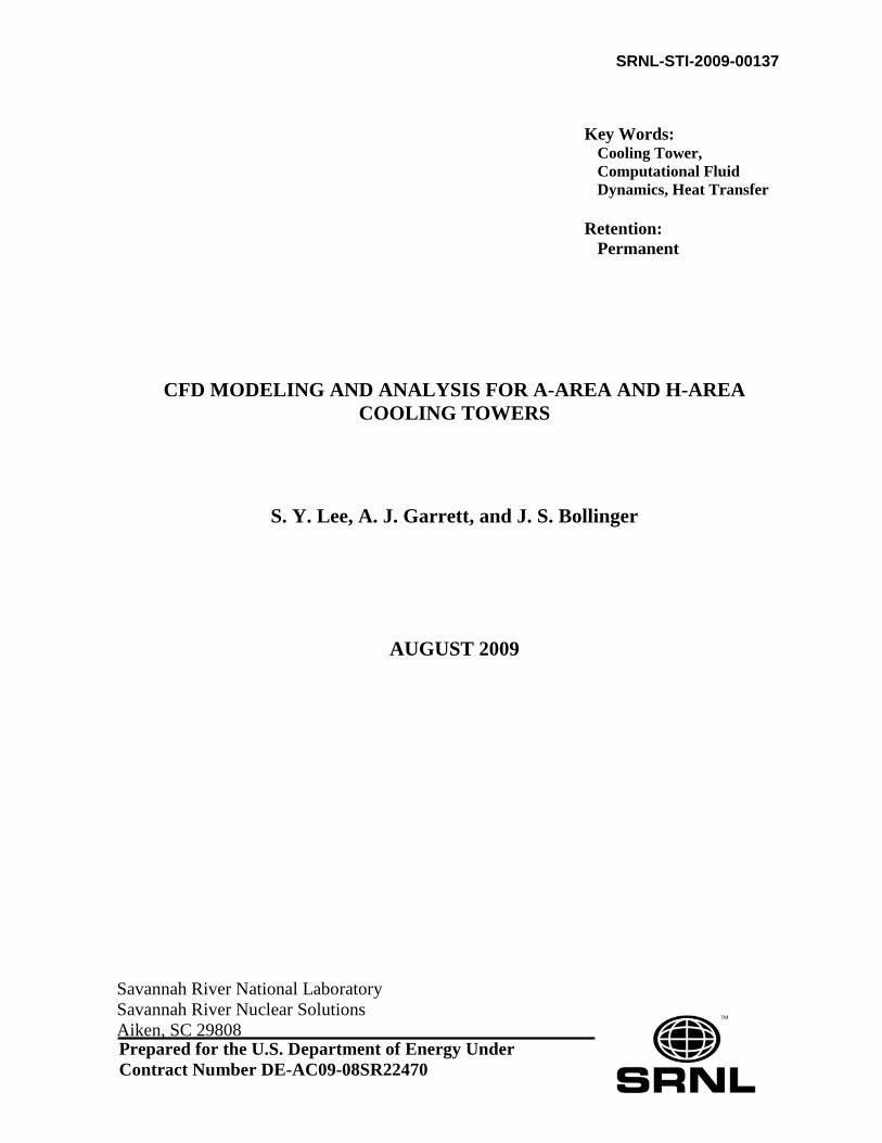
Wind shield Wind shield

Wind shieldWind shield

Cell compartrment wall

1228“

364“

Cell boundary (each cell size: 288“ x 288”)

(1” = 0.0254 m)

Figure 3. Top view showing cell boundary of H-area tower.

Z

Y X

(Cross-flow type MDCT in A-area) (Countercurrent flow type MDCT in H-area)

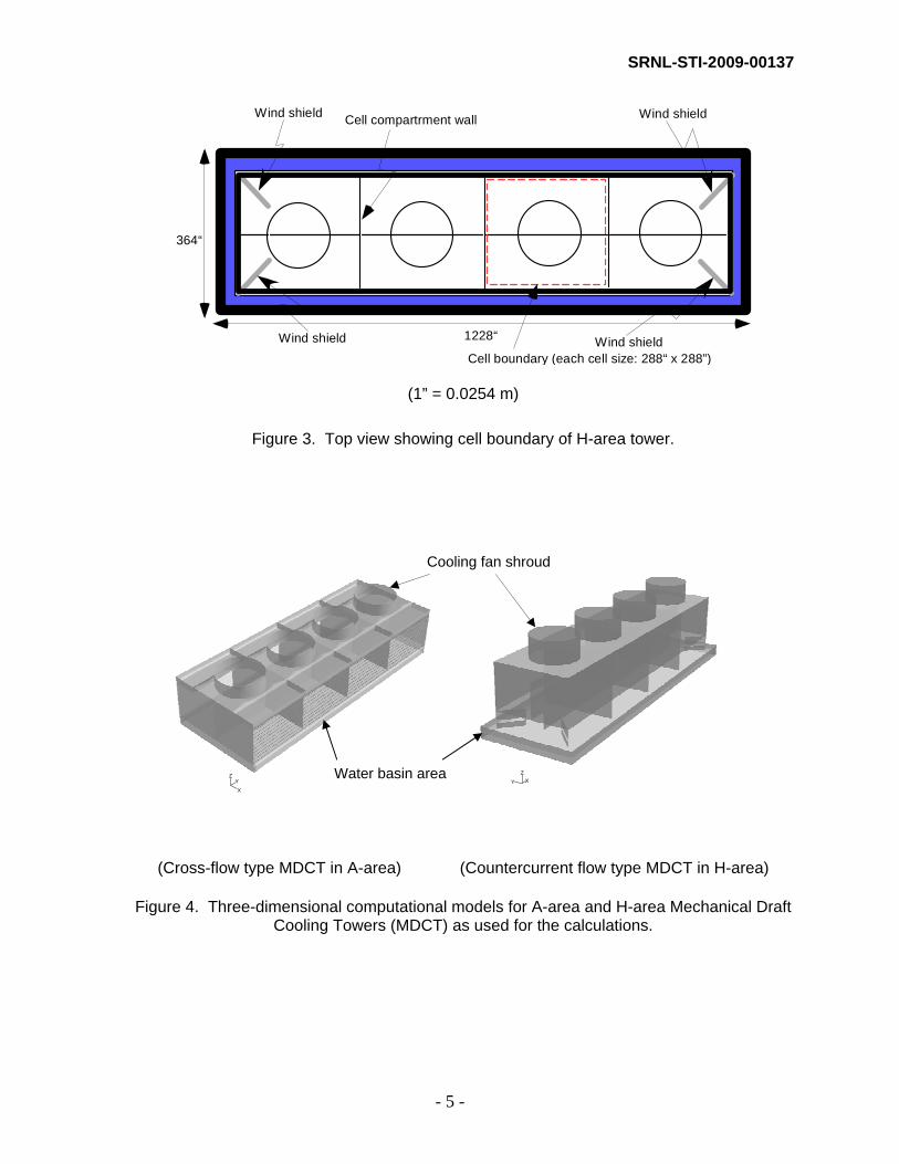
Figure 4. Three-dimensional computational models for A-area and H-area Mechanical Draft

Cooling Towers (MDCT) as used for the calculations.

ZY

X

Cooling fan shroud

Water basin area

SRNL-STI-2009-00137

- 6 -

3.0 MODELING APPROACH AND SOLUTION METHOD The present work took a three-dimensional CFD approach. The modeling domain was parallelepiped, and it was about 8 times larger than the actual size of the four-cell MDCT in Fig. 1 to calculate the air flow patterns inside and outside the tower cells. Cooling fan of each cell was modeled as momentum source at the shroud region since air velocity at shroud exit was continuously measured (only in A-area). The air-vapor mixture model was considered, assuming that vapor phase is always transported by the continuous air phase with no slip. In this situation, water droplet component was considered as discrete phase for the interfacial heat and mass transfer to air via Lagrangian approach as shown in Fig. 5. The force balance for each droplet equates the particle inertia with forces acting on a spherical particle of uniform size, dp. In this work, water distributions at the inlet of the wet deck are assumed to be uniform for computational efficiency although about 20% of non-uniform distributions are shown by the initial test results. Thus, the air-vapor mixture model coupled with discrete water droplet phase is used for the analysis.

Computational cell boundaryof continuous flow domain

Water droplet trajectory

Mass, momentum,energy exchange

Figure 5. Mass, momentum, and heat transfer between the continuous gas phase and discrete water droplet.

The governing equations to be solved for the modeling domain are one air-vapor mixture balance, three momentum conservations, one vapor species transport, along x-, y-, and z- coordinate systems for the modeling domain, turbulence equations, and one air-vapor mixture energy balance. κ−ε standard turbulence model is used for simulation of the turbulent airflow. All governing equations and constitutive relations to be solved for the CFD domain are shown in Eqs. (1) to (28). Droplet momentum balance and heat and mass transfer balance equations, Eq. (8) to (17), are solved by Lagrangian integral approach along the particle trajectory from water droplet inlet to the exit. The modeling constants and

SRNL-STI-2009-00137

- 7 -

gas properties are updated by the constitutive relations as provided by Eqs. (18) to (28). The solution method is summarized in Fig. 6.

The finite volume method with the adoption of an iterative procedure based on semi-implicit method for pressure-linked equations (SIMPLE) of pressure-velocity coupling is used in the present study. The gird distribution was non-uniform with smaller mesh size for the cell regions of the cooling tower as shown in Fig. 7. The present solution is not sensitive to the grid size when the number of total cells is higher than 3 x 106 for the A-Area tower and 2.5 x 106 for the H-Area tower. The iterative solution is considered as converged when the normalized residual errors of all the independent variables solved are reduced at least by three orders and the average exit air temperature is changed less than 0.01 oC. The values of other variables have also been monitored during the iteration to make sure the convergent solution of all the variables at the end of iteration process. Mass conservation equation:

( ) vSv =•∇v

ρ (1) Momentum conservation equation:

( ) ( ) Fgpvvvvvv

++•∇+∇−=•∇ ρτρ (2) Energy conservation equation:

( ){ } ( )vsveffhsm JhTkvhvvv

−∇•∇=+•∇ ,25.0 ρρ (3)

Turbulence equations based on two-equation model:

( ) ( ) ρεµρρ

ρσµµρ +⎟⎟

⎠

⎞⎜⎜⎝

⎛∂∂

⎟⎠

⎞⎜⎝

⎛∂∂

−⎟⎟⎠

⎞⎜⎜⎝

⎛∂

∂−⎟

⎟⎠

⎞⎜⎜⎝

⎛∇⎟⎟

⎠

⎞⎜⎜⎝

⎛+•∇=•∇

it

ti

pi

jji

k

t

xTg

Txu

uukvkPr

1''v (4)

( ) ( ) ⎟⎟⎠

⎞⎜⎜⎝

⎛−

⎥⎥⎦

⎤

⎢⎢⎣

⎡⎟⎟⎠

⎞⎜⎜⎝

⎛∂∂

⎪⎭

⎪⎬⎫

⎪⎩

⎪⎨⎧

⎟⎠

⎞⎜⎝

⎛∂∂

+⎟⎟⎠

⎞⎜⎜⎝

⎛∂

∂⎟⎠

⎞⎜⎝

⎛−⎟⎟⎠

⎞⎜⎜⎝

⎛∇⎟⎟

⎠

⎞⎜⎜⎝

⎛+•∇=•∇

kC

xTg

TC

xu

uuk

Cvit

ti

pi

jji

t2

231 Pr1'' ερµρρ

ρεεσµµρε εεε

ε

v

(5) Species Transport Equation: Conservation equation for vapor species is governed by

( ) vvv SJYv +⋅∇−=⋅∇vv

ρ (6) Yv is local mass fraction of vapor in the continuous air. vJ

v is diffusion flux of vapor species.

Sv in the equation is a source term of vapor species added to the air due to the evaporation of the dispersed water droplets. The diffusion flux of water vapor under turbulent air flow is computed by

vt

tvv Y

ScDJ ∇⎟⎟

⎠

⎞⎜⎜⎝

⎛+−=

µρv

(7)

SRNL-STI-2009-00137

- 8 -

Dv is molecular diffusion coefficient of water vapor in the continuous air medium. Momentum Balance for Discrete Water Droplet Force balance for droplet is considered along the particle trajectory in a Lagrangian reference frame. The force balance equates the particle inertia with forces acting on a spherical particle of uniform size, dp.

xpgxvmxp

pp

ppD

xpgxvmgDip

FFguud

C

FFFFudtd

,,2

,,

Re43

++⎟⎟⎠

⎞⎜⎜⎝

⎛ −+−⎟

⎟

⎠

⎞

⎜⎜

⎝

⎛=

+++=

ρρρ

ρ

(8)

In the above equation, Re and Fvm,x are Reynolds number based on particle diameter dp and additional force due to virtual mass effect, respectively. Coefficient CD in the first term of the right-hand side is drag coefficient on the droplet surface due to the upward air motion. The drag coefficient for the spherical droplet particle as used by FLUENT (Morsi and Alexander, 1972) was applied to the calculations. The last term xpgF , is lift force due to pressure gradient in the fluid side. That is,

µ

ρ pp uud −=Re (9)

( ) 0

21

, ≈−= pp

xvm uudtdF

ρρ since ρp is much larger than the air density ρ. (10)

xuuF p

pxpg ∂

∂=

ρρ

, (11)

Heat and Mass Balance for Discrete Droplet The droplet temperature is updated along the particle trajectory according to a heat balance with no radiation cooling, For boilingpvap TTT <≤

( ) fgp

ppp

pp hdt

dmTThA

dtdT

Cm +−= (12)

Heat transfer coefficient h in the above equation is calculated from a literature correlation [Kessler and Greenkorn, 1999].

315.0

,PrRe6.00.2 d

effh

p

khd

Nu +== (13)

SRNL-STI-2009-00137

- 9 -

Nusselt number, Nu, in Eq. (13) is defined as the ratio of local average convective transfer to conduction-controlled heat transfer, which is very similar to a mass-transfer Sherwood number, Sh, as will be discussed later. Heat transfer coefficient, h, for convective heat flux, the first term in the right-hand-side of Eq. (12), is calculated by the literature correlation Eq. (13). Reynolds number Red is based on the particle diameter dp and the relative velocity as define by Eq. (9). Prandtl number Pr is defined as the ratio of viscous diffusion to conduction for the continuous air phase (Cpµ/k).

Rate of evaporation dt

dmp in Eq. (12) is computed from the mass transfer equation. Mass

transfer at the surface of water droplet is governed by the concentration gradient. The mass flux φ at the surface of each droplet is given by

( )vvpm CCk −=φ (14) In this case the mass concentration of vapor at the droplet surface, Cvp, is estimated by assuming that the partial pressure of vapor at the interface is equal to the saturated vapor pressure, psat, at the droplet temperature, Tp.

( )p

psatvp RT

TpC = , where R is universal gas constant. (15)

The concentration of vapor in the bulk gas, Cv, is known from solution of the transport equation for vapor species when local mole fraction of vapor species is given by Xv at local pressure p and temperature T.

RTpXMC vOHv 2= (16)

where MH2O = molecular weight of water (kg/kgmol) Mass transfer coefficient km in the above equation is calculated from a literature correlation by using the analogy between heat transfer and mass transfer [Kessler and Greenkorn, 1999].

315.0Re6.00.2 Sc

Ddk

Sh dv

pm +== (17)

where Sherwood number, Sh, is defined as the ratio of local average mass transfer to diffusion-controlled mass transfer, which is sometimes called a mass-transfer Nusselt number, Nu. The non-dimensional number, Sc, in the equation is defined as the ratio of viscous to mass diffusion, µ/ρDv, where Dv is diffusion coefficient of vapor in the bulk. Using the mass transfer coefficient, km, calculated by Eq. (17), vapor mass flux φm is computed by Eq. (14). The vapor mass flux becomes a source term of vapor species Sv in the vapor species transport equation Eq. (6). As result of the evaporation of water droplet, the mass of the droplet is reduced after time interval dt according to

SRNL-STI-2009-00137

- 10 -

pmp A

dtdm

φ−= (18)

where mp = mass of the droplet (kg)

Ap = surface area of the water droplet (m2) Change rate of droplet mass due to the evaporation process is coupled with the droplet heat balance equation Eq. (12), resulting in updating the overall energy balance equation for the mixture. Constitutative Relations

• Buoyancy coefficient for turbulent dissipation, C3ε

⎟⎟⎟

⎠

⎞

⎜⎜⎜

⎝

⎛

+=

223 tanhji

k

vv

vC ε (19)

• Turbulent viscosity, µt

⎟⎟⎠

⎞⎜⎜⎝

⎛=

ερµ µ

2kCt (20)

• q’’’ (Amount of sensible heat transfer from water to air inside the cell compartment

excluding the latent of heat under different ambient humidity and operating conditions)

• ρ (Density relations to account for humidity)

Dry air density, ρa, is calculated from the equation of state for ideal gas. That is

RTp

a =ρ (21)

Where p = atmospheric pressure (dynes/cm2) ρa = air density (gm/cm3)

R = gas constant for dry air = 2.8704x106 erg/(gm-K), where 1 calorie = 4.186x107 ergs

T = temperature (K) When vapor mass fraction of the air-vapor mixture, Yv, is computed by the species balance equation, air density including effect of water vapor ρ is obtained by

( )vv

air

YYRTpM

609.1)1( +−=ρ (22)

Humidity ratio γ is computed in terms of partial pressures for water vapor and air.

SRNL-STI-2009-00137

- 11 -

⎟⎟⎠

⎞⎜⎜⎝

⎛

−=⎟⎟

⎠

⎞⎜⎜⎝

⎛−

=⎟⎟⎠

⎞⎜⎜⎝

⎛=⎟⎟

⎠

⎞⎜⎜⎝

⎛⎟⎟⎠

⎞⎜⎜⎝

⎛===

sat

sat

w

w

a

w

a

w

a

w

a

w

a

w

ppp

ppp

pp

pp

MM

mm

φφ

ρργ 622.0622.0622.0 (23)

pw and pa in Eq. (23) are partial pressures for water vapor and air, respectively. By using Dalton’s law, specific humidity γ for a given relative humidity φ is computed in terms of saturation pressure psat.

⎟⎟⎠

⎞⎜⎜⎝

⎛

−=

sat

sat

pppφ

φγ 622.0 (24)

By using Eq. (24), the relationship between vapor mass fraction Yv and relative humidity φ is obtained. The vapor mass fraction is called specific humidity.

⎟⎟⎠

⎞⎜⎜⎝

⎛

−=⎟⎟

⎠

⎞⎜⎜⎝

⎛+

=sat

satv pp

pYφ

φγ

γ378.0

622.01

(25)

The saturated pressure Psat in Eq. (25) is expressed in Pa. The saturation pressure is calculated by Eq. (26) for a temperature T in deg K when water molecular weight MH2O is 18 gm/mol.

⎥⎦

⎤⎢⎣

⎡⎟⎠

⎞⎜⎝

⎛ −=⎥⎦

⎤⎢⎣

⎡⎟⎠

⎞⎜⎝

⎛ −⎟⎠

⎞⎜⎝

⎛=T

LTR

LMp oHsat

115.273

10625.9exp611115.273

1exp611 *2 (26)

where R* = universal gas constant = 8.3144x107 erg/(mol-K), where psat is in unit of Pa. L is latent heat of vaporization in cal/gm, where 1 calorie = 4.186x107 ergs. It is given by L = 597.3 – 0.566(T – 273.15), where T is in deg K. (27) Saturated pressure psat corresponding to droplet temperature, Tp, is computed by Eq. (26). Evaporation temperature, Tvap , is assumed to be saturated at the vapor pressure of the continuous air medium. Note that in the equation above, T will be the ambient dew point temperature if you want to compute the density of the air going into the cooling tower. If you want to compute the density of the air leaving the cooling tower, then T will be the temperature of the air after it has been warmed and moistened by contact with the hot water in the fill zone.

• Momentum Source Term in Flow Momentum Equation, F The present model calculates the superficial velocity based on volumetric flow rate. The porous media model incorporates an empirically determined flow resistance in an isotropic porous region. In essence, the isotropic porous media model is nothing more than an added momentum sink in the governing momentum equation Eq. (2). The source term is composed of two parts, a viscous loss term and an inertial loss term. It was based on Ergun’s equation [3].

⎟⎠

⎞⎜⎝

⎛+−= 2

21

iii vCvF ραµ (28)

SRNL-STI-2009-00137

- 12 -

where ( ) ⎟

⎟

⎠

⎞

⎜⎜

⎝

⎛

−−= 3

32

1150 ε

εα pd , and ( )

⎟⎟

⎠

⎞

⎜⎜

⎝

⎛ −−= 3

15.3ε

ε

pdC .

Fi in Eq. (28) is the momentum sink term in the direction i, where i = 1, 2, or 3, corresponding to the x-, y-, and z-direction, respectively. The coefficients α and C will be determined by the literature data.

• Energy Balance Equation in Porous Media The present model calculates the energy transport equation given by Eq. (3) in porous zone with modifications to the transient terms and the conduction heat flux only. Total energy in the time derivative is used as the fluid-solid mixture energy, which is homogeneously mixed in terms of porosity. Thermal conductivity, kh,eff, used in the conduction heat flux is used as the homogeneous mixture of fluid and solid conductivities.

( ) sfeffh kkk εε −+= 1, (29) kf and ks in Eq. (29) are thermal conductivities for fluid and solid materials in porous media, respectively, assuming isotropic thermal contributions of solid material to the continuous fluid medium. Boundary Conditions: Boundary conditions for the modeling domain are provided for the following:

• Wind speed and direction • Ambient air or dry-bulb temperature • Ambient humidity – vapor mass fraction • Water inlet temperature • Water flow rate • Fan speed • Water basin temperature for cooling tower system

SRNL-STI-2009-00137

- 13 -

Ambient conditions (Wind speed and direction, Temp, Humidity)Water droplet temperatures at inlet, Air velocity at shroud exit

Modified air density dueto evaporation of water

inside cell

Sensible heat to change airtemperature due to heat

transfer from water inside cell

Mass transferfrom water to air

Heat Transfer betweenair and water

1 mass conservation

3 momentum conservations

1 energy conservation2 turbulence equations

Single-component air momentumand energy transport eqs.

1 vapor species transport

Figure 6. Solution methodology for single-phase mixture modeling approach.

SRNL-STI-2009-00137

- 14 -

(3-million nodes for the model of A-Area crossflow cooling tower)

(2.5-million nodes for the model of H-Area counterflow cooling tower)

Figure 7. Computational meshes for the three-dimensional domains representing A-area

and H-area Mechanical Draft Cooling Towers (MDCT).

SRNL-STI-2009-00137

- 15 -

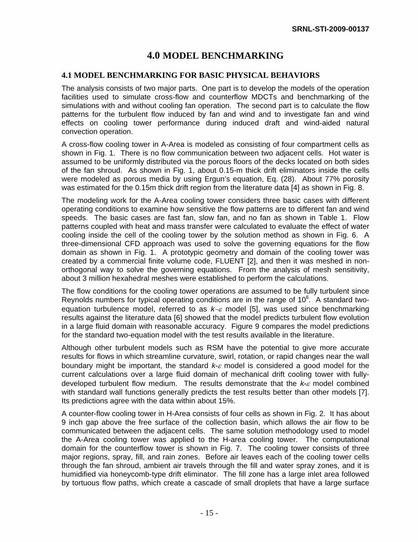
4.0 MODEL BENCHMARKING 4.1 MODEL BENCHMARKING FOR BASIC PHYSICAL BEHAVIORS The analysis consists of two major parts. One part is to develop the models of the operation facilities used to simulate cross-flow and counterflow MDCTs and benchmarking of the simulations with and without cooling fan operation. The second part is to calculate the flow patterns for the turbulent flow induced by fan and wind and to investigate fan and wind effects on cooling tower performance during induced draft and wind-aided natural convection operation.

A cross-flow cooling tower in A-Area is modeled as consisting of four compartment cells as shown in Fig. 1. There is no flow communication between two adjacent cells. Hot water is assumed to be uniformly distributed via the porous floors of the decks located on both sides of the fan shroud. As shown in Fig. 1, about 0.15-m thick drift eliminators inside the cells were modeled as porous media by using Ergun’s equation, Eq. (28). About 77% porosity was estimated for the 0.15m thick drift region from the literature data [4] as shown in Fig. 8.

The modeling work for the A-Area cooling tower considers three basic cases with different operating conditions to examine how sensitive the flow patterns are to different fan and wind speeds. The basic cases are fast fan, slow fan, and no fan as shown in Table 1. Flow patterns coupled with heat and mass transfer were calculated to evaluate the effect of water cooling inside the cell of the cooling tower by the solution method as shown in Fig. 6. A three-dimensional CFD approach was used to solve the governing equations for the flow domain as shown in Fig. 1. A prototypic geometry and domain of the cooling tower was created by a commercial finite volume code, FLUENT [2], and then it was meshed in non-orthogonal way to solve the governing equations. From the analysis of mesh sensitivity, about 3 million hexahedral meshes were established to perform the calculations.

The flow conditions for the cooling tower operations are assumed to be fully turbulent since Reynolds numbers for typical operating conditions are in the range of 106. A standard two-equation turbulence model, referred to as k−ε model [5], was used since benchmarking results against the literature data [6] showed that the model predicts turbulent flow evolution in a large fluid domain with reasonable accuracy. Figure 9 compares the model predictions for the standard two-equation model with the test results available in the literature.

Although other turbulent models such as RSM have the potential to give more accurate results for flows in which streamline curvature, swirl, rotation, or rapid changes near the wall boundary might be important, the standard k-ε model is considered a good model for the current calculations over a large fluid domain of mechanical drift cooling tower with fully-developed turbulent flow medium. The results demonstrate that the k-ε model combined with standard wall functions generally predicts the test results better than other models [7]. Its predictions agree with the data within about 15%.

A counter-flow cooling tower in H-Area consists of four cells as shown in Fig. 2. It has about 9 inch gap above the free surface of the collection basin, which allows the air flow to be communicated between the adjacent cells. The same solution methodology used to model the A-Area cooling tower was applied to the H-area cooling tower. The computational domain for the counterflow tower is shown in Fig. 7. The cooling tower consists of three major regions, spray, fill, and rain zones. Before air leaves each of the cooling tower cells through the fan shroud, ambient air travels through the fill and water spray zones, and it is humidified via honeycomb-type drift eliminator. The fill zone has a large inlet area followed by tortuous flow paths, which create a cascade of small droplets that have a large surface

SRNL-STI-2009-00137

- 16 -

area for upward airflow and fallen water droplets. Based on the product information for a 19-mm standard gap spacing [13], the fill medium in the model was assumed to be a porous media with 90% porosity to consider tortuous flow path and large surface area.

The literature correlation [8] was used to calculate the heat and mass transfer from water droplets to the continuous gas phase at steady state, assuming them to be spherical and uniform. Based on the literature information [10] and SRS experimental observation, the model used the fixed droplet diameter to be 1 mm for the present analysis. Yao and Schrock [11] performed the experimental work to measure the temperature drops for 3 to 5 mm diameter ranges of water droplets falling through a 3m column containing the conditioned air. As shown in Fig. 10, the present model was benchmarked against the test results. The calculation results show that when single droplet has 6 mm diameter, the model under predicts the data by about 18% on the average since the current model assumes spherical droplet. The experimental observations [11] clearly show that when a droplet is larger than 4mm, it becomes non-spherical during free fall.

Air velocity (ft/sec)

Pre

ssu

red

rop

(Pa)

0 2 4 6 8 10 12 14 160

10

20

30

40

50

60

70

80

90

100

Literature data (by Tech Sales Co.)

Predictions (by Ergun’s equation)

Figure 8. Comparison of the pressure drops across the drift eliminator with the literature

data (77% porosity).

SRNL-STI-2009-00137

- 17 -

yx

z

H

t

W

Lh

Air

Air

y = 2H

A

A’

Non-dimensional distance (z/H)

No

n-d

imen

sio

nal

velo

city

(u/U

o)

0 0.2 0.4 0.6 0.8 1-0.6

-0.4

-0.2

0

0.2

0.4

0.6

0.8

1

Nielsen et al. [6]Standard two-equation turbulence model

y = 2H, x = 2.35HRe = 7,100 (inlet flow condition)

(L/H = 3.1, W/H = 4.7, h/H = 0.056, t/H = 0.16, H = 0.0893 m)

Figure 9. Benchmarking results of non-dimensional horizontal air velocity along the line A-A’

on the plane of y=2H distance from the air inlet plane at Re = 7,100 inlet flow (inlet air velocity, U = 10.371 m/sec).

A’ A

SRNL-STI-2009-00137

- 18 -

Falling distance from water droplet inlet (m)

Tem

per

atu

red

rop

ofw

ater

dro

ple

t(d

egC

)

0 0.5 1 1.5 2 2.5 30

1

2

3

4

5

6

7

8

9

10

Test data - 4mm droplet [Yao, 1976]

Model predictions - 4mm droplet

Air temp = 22 deg C36% Relative humidity





Droplet size = 3 mm

Droplet size = 4 mm

Droplet size = 6 mm

Figure 10. Comparison of the predicted droplet cooling with the test data for free-falling

water droplet in still air [10]. 4.2 INTEGRAL BENCHMARKING RESULTS FOR A-AREA

Test Descriptions for Experimental Measurement The second compartment cell of the four-cell cross-flow MDCT at Savannah River Site (SRS) was instrumented at the exit of the shroud region and near the water collection basin. Sensor locations for the measurements of key operating parameters are shown in Fig. 11. Air temperature and relative humidity measurements were made by using a HOBO data logger [1] at six locations near the top of the cooling fan shroud. Water temperatures at the tower exit were also measured by waterproof Tidbit data logger at 0.7 m above the free surface of the collection basin. Water flow rate and temperature at the inlet of the distribution deck were measured by Doppler ultrasonic flow meter and Tidbit, respectively. Measurement data for each sensor location were recorded at a time interval of 15 minutes during a two-month period in 2006. Test data for ambient air temperature and relative humidity including wind speed and direction at the inlet of the second cell were continuously obtained from meteorology stations located north and south of the cooling tower. Wind speed and direction were measured by the A-Wind tower. The data recorded by the data logger were downloaded to a computer and then averaged over 1-hour periods for the benchmarking database used to validate the model. The relative humidity measurements were converted to specific humidity or vapor mass fraction values. The measurement conditions for each test case are summarized in Table 1. Test results were used to benchmark and validate the model.

SRNL-STI-2009-00137

- 19 -

Modeling predictions for turbulent airflow behavior and heat transfer characteristics were benchmarked against the literature data using simple geometrical systems. The verified model was extended to the prototypic MDCT system coupled with air humidification process to perform the integral benchmarking tests. The test cases for the SRS cooling tower consist of three basic cases. From the literature information [10] shown in Fig. 12, droplet size for the A-Area cooling tower was used to be 1 mm diameter for the present calculations since it has an array of thin-rectangular splashing plate inside the cooling cell. As shown in Table 1, there are typically three different air velocities at the shroud exit, depending on the fan speeds of the cooling tower. Average computational time for each of the test cases was about 4 days for a two-cpu parallel run under HP DL585 Linux IBM workstation (IBM).


LouverLouver

Water Water

Air out (uex)

Air Air

Centraldivider wall

Air

A B

Air

CL

0.4096m

1.597m

1.724m

3 m1.2 m1.2 m0.7 m 3 m 1.2 m1.2 m

Air temp. and humidity sensor locationWater temp. measurement location

Plantnorth(PN)

PN

(Top view ofthe instrumentedfan shroud exit)

Figure 11. Cross-section view of the compartment cell instrumented for the performance measurement for A-area cooling tower.

SRNL-STI-2009-00137

- 20 -

Table 1. Test conditions and results for the A-Area MDCT

Ambient conditions Test cases

vex

(m/s) Tamb (oC), Yv,amb Uo(m/s)*, θo

Twi (oC)

Fast1 7.76 16.17, 0.0106 2.14, 85.5 27.78

Fast2 7.72 16.78, 0.0081 6.41, 298.2 27.12

Fast3 7.83 22.18, 0.0125 5.69, 263.5 31.78

Slow1 5.20 11.54, 0.0081 3.36, 306.8 26.90

Slow2 5.20 11.43, 0.0081 2.33, 291.80 26.96

Slow3 5.11 12.94, 0.0082 4.64, 301.3 27.06

Slow4 5.06 17.11, 0.0082 4.98, 299.8 27.92

Slow5 5.12 14.56, 0.0080 5.10, 294.3 27.07

Nofan1 -0.55 11.55, 0.0083 3.32, 305.4 26.79

Nofan2 0.24 11.36, 0.0080 2.88, 287.3 26.88

Nofan3 0.33 12.11, 0.0083 3.27, 291.0 26.95

Nofan4 0.37 16.24, 0.0080 5.23, 296.5 27.01

Nofan5 0.14 13.5, 0.0080 5.46, 303.5 26.80

Note:*Averaged value

SRNL-STI-2009-00137

- 21 -

Upward air flow velocity (m/sec)

Wat

erd

rop

letd

iam

eter

(mm

)

1 2 3 4 5 6 7 810-2

10-1

100

101

102

103

104

Max. possible droplet diameter [Fisenko et al., 2004]Min. possible droplet diameter [Fisenko et al., 2004]

Present analysis

Ranges of upward air velocities inside the cell

Droplet size used for H-Area tower

Droplet size used for A-Area tower

Figure 12. Possible range of droplets sizes for various upward flow air velocities.

The modeling predictions for air velocity around the cooling tower under the Fast1 conditions are compared with the test results obtained from the SRNL meteorology station as shown in Table 2. The results show that the predictions reasonably agree with the test data. Figure 13 compares the predicted air temperatures at the shroud exit with the test results for the Fast1 test condition. As shown in the figure, air temperature at the southwestern side of the shroud exit is very close to the ambient temperature. It may be caused by downwash mixed in ambient air through the fan motor housing, which was not included in the model. The corresponding results for the vapor mass fraction at the shroud exit are shown in Fig. 14. The results show that the model predictions are in agreement with the test data within 15%. As shown in the figure, air temperature at the center of the shroud exit is lower than the peripheral region, which is consistent with the test data. This is mainly due to the higher air velocity at its center so that air phase has smaller contact time with the warmer water phase when air velocity becomes higher as shown in Fig. 15. The air temperature and vapor mass fraction distributions at the vertical plane crossing the second cell are shown in Figs. 16 and 17, respectively. The results show that air temperature increases by about 4oC and humidity increases by about 8% RH (RH or vapor mass fraction?) through the cooling tower. Table 3 shows quantitative comparison of the water exit temperatures between the model predictions and the test data under the Fast1 test condition. As shown in the table, the predicted water temperature at the tower exit is about 6% lower than the data on average.

SRNL-STI-2009-00137

- 22 -

Table 2. Comparison of wind velocity predictions around the cooling tower with test data under the Fast1 conditions

Wind speed (m/sec) Directions (angle) Locations

Predictions Data Predictions Data

Upstream side (North)

1.60 1.35 24.5 29.0*

Downstream side (South)

2.20 1.54 64.1 70.9*

Note: *Both wind directions are toward the cooling tower.

The scoping calculations were based on the model with no flow obstructions near the cooling tower. A storage shed is located 32 inches from the northern side of the 2nd cell. The shed is 8.3 ft wide, 16.7 ft long, and 8.3 ft high. Figure 18 shows a comparison of air velocity distributions between the models with and without the shed at the horizontal plane 4 ft above the ground surface for Fast1 case. The vapor mass fraction distributions of the model with the shed are compared with the one without the shed obstruction at the mid-plane of 2nd cell for the same case in Fig. 19. The results show that there is little impact on the cooling tower performance with the presence of small storage shed. Figure 20 presents temperature distributions of water droplets for the Fast1 test condition.

When cooling fans are turned off, water droplets inside each cell will be cooled by wind, natural convection and sensible heat transfer. As shown in Figs. 21 and 22, the modeling predictions for the air temperature and specific humidity profile at the exit plane of the fan shroud are compared with the test results for the NoFan5 test condition. In this case, the wind direction was northwestern as shown in Table 1. The test results clearly show that when cooling fans are off, air temperatures at the shroud exit are nearly uniform. It is noted that the modeling predictions for Nofan5 have non-zero gradients over the distance from the upstream (north) side of wind to the downstream (south) side since the model did not consider detailed flow obstructions such as splashing plates inside each cell. Thus, the predicted temperatures at the upstream side are slightly lower than the downstream side because of the smaller residence time of air inside the cell. The overall discrepancy between the model predictions and the test data is less than about 10%.

The variations of exit air and water temperatures with air mass flow rate are shown in Figs. 23 and 24, respectively. The test results show that the distribution of exit water temperatures are non-uniform for a given air flow rate. By visual inspection of the A-Area cooling tower from the side and from above, the falling rain is not uniform in droplet size and there is poor flow distribution below the spray zone. The overall predictions are in reasonable agreement with the test results. As shown in the figures, it is noted that the exit air temperature tends to decrease with increasing air mass flow rate, and the exit water temperature decreases as air mass flow rate increases. The performance of a mechanical draft cooling tower can be evaluated in terms of the approach of the exit water temperature to the ambient wet-bulb temperature. The cooling tower performance or temperature ratio is defined in Eq. (30) as

inwbainw

outwinw

TTTT

R,,,

,,

−−

= (30)

SRNL-STI-2009-00137

- 23 -

where Tw,in is the inlet water temperature, Tw,out is the outlet water temperature and Ta,wb,in is the ambient wet-bulb temperature. At given inlet air and inlet water temperatures, and water mass flow rate, the temperature ratio increases with increasing air mass flow rate as shown in Fig. 25.

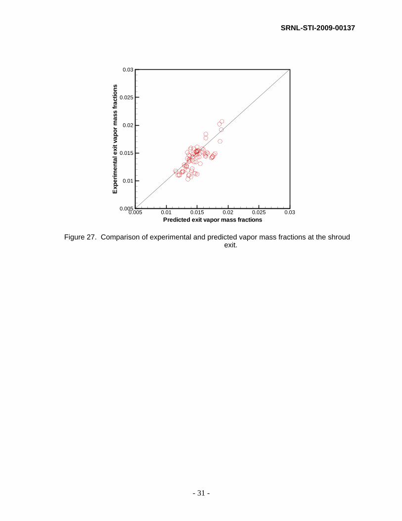
A comparison of the experimental and predicted air temperatures and vapor mass fractions at the shroud exit are shown in Figs. 26 and 27, respectively. The root-mean-square (RMS) errors in air temperatures and vapor mass fractions are 11% and 12%, respectively . Some of the discrepancy between experimental and predicted results can be attributed to the water flow maldistribution on the decking material below the spray zone. It is concluded that the CFD model for the MDCT system captures basic flow patterns and heat transfer characteristics, and it predicts the test results in a reasonably accurate way.

Distance from center (m)

Tem

pera

ture

(deg

C)

-3 -2 -1 0 1 2 35

10

15

20

25

30

35

Predictions - East sidePredictions - West side

North side South side

Test data - East side

Test data - West side

Ambient temperature

Figure 13. Comparison of the air temperature profile at the shroud exit for the Fast1 test condition.

SRNL-STI-2009-00137

- 24 -

Position from center (m)

Vap

orm

ass

frac

tion

-3 -2 -1 0 1 2 30.005

0.01

0.015

0.02

0.025Predictions - East side

Predictions - West side



Ambient vapor mass fraction

Figure 14. Comparison of the vapor mass fraction profile at the shroud exit for the Fast1

test condition.

Velocity Vectors Colored By Velocity Magnitude (m/s)

FLUENT 6.2 (3d, segregated, spe, ske)

Oct 18, 2007

9.23e+00

8.75e+00

8.28e+00

7.80e+00

7.32e+00

6.84e+00

6.37e+00

5.89e+00

5.41e+00

4.93e+00

4.46e+00

3.98e+00

3.50e+00

3.02e+00

2.55e+00

2.07e+00

1.59e+00

1.11e+00

6.37e-01

1.60e-01

Z

Y X

Figure 15. Air flow patterns at the vertical mid-plane crossing the instrumented cell of the

cooling tower for the Fast1 test condition.

SRNL-STI-2009-00137

- 25 -

Contours of t_degc


Feb 29, 2008

2.61e+01

2.56e+01

2.51e+01

2.46e+01

2.41e+01

2.36e+01

2.31e+01

2.26e+01

2.21e+01

2.16e+01

2.11e+01

2.06e+01

2.01e+01

1.96e+01

1.91e+01

1.86e+01

1.81e+01

1.76e+01

1.71e+01

1.66e+01

1.61e+01

Z

Y X

Figure 16. Air temperature distribution at the vertical mid-plane crossing the instrumented

cell of the cooling tower for Fast1 test condition.

Contours of Mass fraction of h2o


Oct 18, 2007

2.13e-02

2.08e-02

2.02e-02

1.97e-02

1.92e-02

1.86e-02

1.81e-02

1.75e-02

1.70e-02

1.64e-02

1.59e-02

1.53e-02

1.48e-02

1.43e-02

1.37e-02

1.32e-02

1.26e-02

1.21e-02

1.15e-02

1.10e-02

Z

Y X

Figure 17. Vapor mass fractions at the vertical mid-plane crossing the instrumented cell of

the cooling tower for Fast1 test condition,.

SRNL-STI-2009-00137

- 26 -

Contours of Velocity Magnitude (m/s)


Feb 26, 2007

4.20e+00

3.99e+00

3.78e+00

3.57e+00

3.36e+00

3.15e+00

2.94e+00

2.73e+00

2.52e+00

2.31e+00

2.10e+00

1.89e+00

1.68e+00

1.47e+00

1.26e+00

1.05e+00

8.40e-01

6.30e-01

4.20e-01

2.10e-01

0.00e+00

ZY

X

Contours of Velocity Magnitude (m/s)


Oct 18, 2007

4.20e+00

3.98e+00

3.76e+00

3.54e+00

3.32e+00

3.09e+00

2.87e+00

2.65e+00

2.43e+00

2.21e+00

1.99e+00

1.77e+00

1.55e+00

1.33e+00

1.11e+00

8.84e-01

6.63e-01

4.42e-01

2.21e-01

0.00e+00

ZY

X

Figure 18. Comparison of air velocity distributions between the models with and without the shed at the horizontal plane 4 ft above the ground surface for the Fast1 test condition.



Feb 26, 2007

2.14e-02

2.09e-02

2.04e-02

1.99e-02

1.94e-02

1.88e-02

1.83e-02

1.78e-02

1.73e-02

1.67e-02

1.62e-02

1.57e-02

1.52e-02

1.47e-02

1.41e-02

1.36e-02

1.31e-02

1.26e-02

1.21e-02

1.15e-02

1.10e-02

Z

Y X



Oct 18, 2007

2.13e-02

2.08e-02

2.02e-02

1.97e-02

1.92e-02

1.86e-02

1.81e-02

1.75e-02

1.70e-02

1.64e-02

1.59e-02

1.53e-02

1.48e-02

1.43e-02

1.37e-02

1.32e-02

1.26e-02

1.21e-02

1.15e-02

1.10e-02

Z

Y X

Figure 19. Comparison of vapor mass fraction distributions between the models with and

without the shed at the mid-plane of 2nd cell for the Fast1 test condition.

SRNL-STI-2009-00137

- 27 -

Particle Traces Colored by t_degc


Feb 27, 2007

2.78e+01

2.72e+01

2.66e+01

2.60e+01

2.54e+01

2.48e+01

2.42e+01

2.37e+01

2.31e+01

2.25e+01

2.19e+01

2.13e+01

2.07e+01

2.02e+01

1.96e+01

1.90e+01

1.84e+01

1.78e+01

1.72e+01

1.67e+01

1.61e+01

Z

YX

Figure 20. Temperature distributions of water droplets for the Fast1 test condition.

Table 3. Comparison of water temperature predictions with test data at 28-in above the water basin surface for the Fast1 test condition.

Temperature (oC) Locations

Predictions Test data

North outer 18.40 19.32

North middle 19.72 22.74

North inner 22.00 24.72

South outer 19.01 18.65

South middle 20.54 21.14

South inner 21.82 22.76

Average 20.25 21.55

Plant North

SRNL-STI-2009-00137

- 28 -

Distance from the center (m)

Tem

pera

ture

(deg

C)

-3 -2 -1 0 1 2 35

10

15

20

25

30

35

Predictions - East sidePredictions - West side



North side Southe side

Ambient temperature

Figure 21. Comparison of the air temperature profile at the shroud exit for the Nofan5 test condition.

Distance from the center (m)

Vap

or

mas

sfr

actio

ns

-3 -2 -1 0 1 2 30.005

0.01

0.015

0.02

0.025

Predictions - East side

Predictions - West side



Ambient vapor mass fraction

Figure 22. Comparison of the vapor mass fraction profile at the shroud exit for the Nofan5 test condition.

SRNL-STI-2009-00137

- 29 -

Air mass flowrate through the cell exit (kg/sec)

Air

tem

per

atu

reat

shro

ud

exit

(deg

C)

0 50 100 150 200 250 3005

10

15

20

25

30

35

40

Test data for Nofan4Test data for Slow4Test data for Fast1

Modeling predictions

Average air temperature

Ambient air temperature

Water flowrate = 62 kg/sec

Figure 23. Variation of exit air temperature with air mass flow rate.

Air mass flowrate through the cell exit (kg/sec)

Wat

erte

mp

erat

ure

atex

it(d

egC

)

0 50 100 150 200 250 3005

10

15

20

25

30

35

40

Test data for Nofan4Test data for Slow4Test data for Fast1

Modeling predictions

Average water temperature at exit

Water temperature at inlet


Figure 24. Variation of exit water temperature with air mass flow rate.

SRNL-STI-2009-00137

- 30 -

Air mass flowrate (kg/sec)

Vap

or

mas

sfr

actio

nin

air

0 50 100 150 200 250 3000

0.005

0.01

0.015

0.02

0.025

0.03Test resultsModeling predictionsAmbient conditions

(100% humidity)

(100% humidity)(100% humidity)

(69% humidity) (67% humidity)(67% humidity)


Ambient air temperature = 16.5 deg CWater inlet temperature = 27.4 deg C

Figure 25. Variation of A-Area cooling tower performance with air mass flow rate.

Predicted exit air temperature (deg C)

Exp

erim

enta

lexi

tair

tem

pera

ture

(deg

C)

10 15 20 25 30 3510

15

20

25

30

35

Figure 26. Comparison of experimental and predicited air temperatures at the shroud exit.

SRNL-STI-2009-00137

- 31 -

Predicted exit vapor mass fractions

Exp

erim

enta

lexi

tvap

orm

ass

frac

tions

0.005 0.01 0.015 0.02 0.025 0.030.005

0.01

0.015

0.02

0.025

0.03

Figure 27. Comparison of experimental and predicted vapor mass fractions at the shroud

exit.

SRNL-STI-2009-00137

- 32 -

Table 4. Test conditions and results for the A-Area MDCT.

Air temperature at exit (oC) Vapor mass fraction at exit, Yv,ex

Test cases

Tamb (oC), Yv,amb

Test data Pred. % error Test data Pred. % error 19.05 19.51 2.4 0.0137 0.0142 3.618.43 19.81 7.5 0.0133 0.0145 9.017.85 18.14 1.6 0.0128 0.0129 0.817.78 18.27 2.8 0.0125 0.0130 4.020.59 19.82 3.7 0.0148 0.0145 2.0

Fast1 16.17, 0.0106

17.21 19.54 13.5 0.0120 0.0142 18.317.31 20.12 16.2 0.0125 0.0133 6.418.45 20.22 9.6 0.0140 0.0134 4.317.52 18.25 4.2 0.0118 0.0115 2.517.86 18.31 2.5 0.0116 0.0116 0.019.00 20.32 6.9 0.0139 0.0137 1.4

Fast2 16.78, 0.0081

16.68 20.19 21.0 0.0119 0.0135 13.424.66 25.40 3.0 0.0202 0.0186 7.923.71 25.59 7.9 0.0192 0.0189 1.623.57 23.49 0.3 0.0184 0.0164 10.923.72 23.51 0.9 0.0177 0.0164 7.324.63 25.64 4.1 0.0207 0.0190 8.2

Fast3 22.18, 0.0125

22.78 25.46 11.8 0.0171 0.0187 9.415.41 18.08 17.3 0.0109 0.0137 24.518.37 18.04 1.8 0.0136 0.0137 0.714.91 16.26 9.1 0.0109 0.0121 9.015.44 16.28 5.4 0.0109 0.0121 10.019.69 18.81 4.3 0.0141 0.0143 0.0

Slow1 11.54, 0.0081

15.32 18.53 21.0 0.0106 0.0138 29.016.02 17.91 11.8 0.0110 0.0136 23.618.09 18.02 0.4 0.0136 0.0137 0.715.21 15.97 5.0 0.0110 0.0119 8.215.57 16.00 2.8 0.0110 0.0119 8.218.85 18.05 4.1 0.0135 0.0137 1.5

Slow2 11.43, 0.0081

14.97 17.82 19.0 0.0103 0.0133 29.116.32 19.35 18.6 0.0114 0.0145 27.218.79 19.03 1.3 0.0143 0.0142 0.015.83 17.49 10.5 0.0116 0.0127 9.516.17 17.44 7.9 0.0117 0.0127 8.519.51 20.26 4.0 0.0143 0.0153 7.0

Slow3 12.94, 0.0082

16.00 19.98 24.9 0.0112 0.0145 29.517.90 21.39 19.5 0.0134 0.0148 10.420.38 21.08 3.4 0.0158 0.0144 8.918.42 19.78 7.4 0.0127 0.0133 4.718.90 19.75 4.5 0.0126 0.0132 3.920.86 22.06 5.8 0.0158 0.0158 0.0

Slow4 17.11, 0.0082

17.90 21.80 21.8 0.0131 0.0155 18.3

SRNL-STI-2009-00137

- 33 -

Table 4. Test conditions and results for the A-Area MDCT (continued)

Air temperature at exit (oC) Vapor mass fraction at exit, Yv,ex Test cases

Tamb (oC), Yv,amb

Test data Pred. % error Test data Pred. % error 17.27 19.76 14.4 0.0118 0.0141 19.519.19 19.43 1.3 0.0146 0.0138 4.816.65 18.11 8.8 0.0117 0.0126 7.716.95 18.05 6.5 0.0115 0.0125 8.719.54 20.58 5.3 0.0142 0.0150 5.6

Slow5 14.56, 0.0080

16.36 20.26 23.8 0.0113 0.0145 28.321.56 19.71 8.6 0.0161 0.0150 6.820.89 19.50 6.7 0.0152 0.0148 2.620.19 21.68 7.4 0.0148 0.0164 10.820.37 21.40 5.1 0.0149 0.0162 8.719.76 22.85 15.6 0.0143 0.0175 22.4

Nofan1 11.55, 0.0083

19.73 22.60 14.5 0.0141 0.0173 22.720.81 19.54 6.1 0.0152 0.0150 1.320.61 19.38 6.0 0.0152 0.0149 2.019.70 21.41 8.7 0.0144 0.0164 13.919.97 21.33 6.8 0.0145 0.0163 12.419.94 22.60 13.3 0.0144 0.0175 21.5

Nofan2 11.36, 0.0080

19.70 22.51 14.3 0.0142 0.0174 22.521.01 19.91 5.2 0.0154 0.0151 1.921.01 19.76 5.9 0.0155 0.0150 3.220.31 22.02 8.4 0.0149 0.0167 12.120.72 21.79 5.2 0.0151 0.0166 9.920.25 23.26 14.9 0.0149 0.0179 20.1

Nofan3 12.11, 0.0083

20.31 23.04 13.4 0.0147 0.0177 20.421.28 20.78 2.3 0.0159 0.0140 11.920.95 20.70 1.2 0.0157 0.0139 11.520.95 21.79 4.0 0.0154 0.0152 1.321.13 21.59 2.2 0.0153 0.0150 2.020.52 22.41 9.2 0.0156 0.0160 2.6

Nofan4 16.24, 0.0080

20.77 22.27 7.2 0.0152 0.0158 3.920.64 19.20 7.0 0.0147 0.0136 7.520.62 19.03 7.7 0.0152 0.0134 11.320.33 20.41 0.4 0.0146 0.0147 0.020.62 20.03 2.9 0.0148 0.0143 3.420.53 21.06 2.6 0.0149 0.0154 3.4

Nofan5 13.5, 0.0080

20.61 20.72 0.5 0.0148 0.0150 1.4

SRNL-STI-2009-00137

- 34 -

4.3 INTEGRAL BENCHMARKING RESULTS FOR H-AREA All compartment cells of the four-cell counterflow MDCT at H-Area were instrumented at the exit of the shroud region and near the water collection basin. Air temperature and relative humidity measurements were made by using a HOBO data logger [1] at four locations near the top of cooling fan shroud. The measurement sensors were located at the northwestern top corner of each compartment cell about 1 ft above the drift eliminator as shown in Fig. 2. Water temperatures at the cell exit were also measured by waterproof Tidbit data loggers near the free surface of the collection basin. Water flow rate and temperature at the inlet of the water supply to the tower were measured by Doppler ultrasonic flow meter and Tidbit, respectively. Measurement data for each sensor location were recorded at a time interval of 15 minutes during a two-month period in 2005. Sensor locations for exit air temperature, exit relative humidity, inlet and exit water temperatures are presented in Fig. 28. The relative humidity measurements were converted to specific humidity or vapor mass fraction values. When the cooling fan is operated, the air speed at the exit of the fan shroud is about 10 m/sec. Test data for ambient air temperature and relative humidity including wind speed and direction were continuously obtained from the meteorology station. Wind speed and direction were measured by the wind tower station at H-Area. The data recorded by the data logger were downloaded to a computer, and then averaged over 1-hour periods for the benchmarking database used to validate the model. The ambient conditions and measurement results for the H-Area MCCT’s are summarized in Table 5. The measurement results for the H-Area cooling towers were used to benchmark the model.

The velocity field at the plane crossing the vertical center of the 3rd cell under low-speed wind of 0.95 m/sec for the Aug28 case is shown in Fig. 29. It is noted that the air plume direction does not change due to the ambient wind. The corresponding air temperature and vapor mass fraction distributions in the plume are shown in Figs. 30 and 31, respectively. As the wind speed increases to about 2 m/sec, the bouyant plume from the 2nd tower cell begins to bend in the direction of the wind as shown in Fig. 32. The air temperature and vapor mass fraction distributions in the plume under higher wind speed are shown in Figs. 32 and 33, respectively.

Under certain operating conditions, the cooling fans are turned off, resulting in natural convective cooling of the water. Figure 35 compares the velocity fields between the induced draught (fan-on) and natural draught (fan-off) cells during the ambient conditions of the Dec5. Comparison of the air temperature and vapor mass fraction distributions between the fan-on and fan-off cells are made in Figs. 36 and 37, respectively.

Figure 38 makes a comparison of the velocity fields between the low and high wind speed conditions during the fan-off cell operation. The corresponding distributions of the air temperature at the vertical mid-plane of the fan-off cell are compared in Fig. 39. It is noted that when the wind speed increases, the air temperature inside the fan-off cell is distributed in a more asymmetrical way across the upstream and downstream sides due to better mass transfer between the water droplets and air. Water droplet temperatures were calculated along the trajectory within each cell via a Lagrangian approach, assuming droplet size to be uniform and 3 mm diameter. The water droplet temperature distribution is shown in Fig. 40. Figure 41 compares the predicted and measured exit air temperatures for the H-area cooling tower. The corresponding vapor mass fractions at the exit of the H-area cooling tower are compared in Fig. 42. Detailed comparisons of the exit air temperature and vapor mass fractions are made quantitatively in Tables 6 and 7, respectively. The results show that the model can predict the exit air temperatures and vapor mass fractions with a maximum error of 15%.

SRNL-STI-2009-00137

- 35 -

Wind shield Wind shield

Wind shieldWind shield

Cell compartrment wall

1228“

364“

Cell boundary (each cell size: 288“ x 288”)(Top view)

Water droplet inlet

Drift eliminator

Fan shroud

Water collection basin (about 23“ deep)

Fill

Wind shield (only four bottomcorner)Air Air

Air Air

173“ diameter 83“ (height)

47“

6“

43“

69“

12“

34“

10“

20“9“ gap

Side wind shield

46“

Concrete wallWind shield (only four bottomcorner)

288“38“ 38“

12"

(Vertical view)

Air temp. and humidity sensor locationWater temp. measurement location

Figure 28. Cross-section view of the compartment cell instrumented for the performance

measurement of the H-area cooling tower (1” = 0.0254 m).

SRNL-STI-2009-00137

- 36 -

Table 5. Ambient conditions and measurement results for the H-Area MDCT’s. Ambient conditions Twi mw Tcell, exit (oC), RH, (fan on:1, fan off:0) Test

cases (2005)

Tamb (oC) RH

Uo(m/s), θo

(oC) kg/sec 1st cell 2nd cell 3rd cell 4th cell

July21 24.40 0.86 0.71, 222.9 28.02 329.4 25.67, 0.99, (1)

25.56,1.0, (1)

25.23,1.0, (1)

28.02, 0.99, (1)

July22 25.17 0.80 0.81, 215.7 27.84 329.41 25.69, 0.98, (1)

25.56, 0.97, (1)

25.17, 0.96, (1)

25.17, 0.98, (1)

July26 28.22 0.68 1.0, 188.6 28.92 337.2 27.21, 0.98, (1)

26.73, 1.0, (1)

26.73, 1.0, (1)

26.73, 0.95, (1)

Aug8 27.44 0.77 1.25, 224.5 28.05 319.42 26.34, 0.97, (1)

26.34, 1.0, (1)

26.02, 1.0, (1)

26.03, 1.0, (1)

Aug14a 24.01 0.94 1.34, 169.4 26.15 316.1 24.40, 0.98, (1)

24.27, 0.97, (1)

24.08, 0.99, (1)

24.40, 0.99, (1)

Aug28 24.40 0.94 0.95, 55.66 27.56 449.2 25.95, 0.98, (1)

25.56, 0.99, (1)

25.46, 0.99, (1)

25.66, 1.0, (1)

Sep2 21.33 0.81 1.32, 343.8 22.72 416.8 21.71, 0.96, (1)

21.33, 0.95, (1)

21.14, 0.95, (1)

21.33, 0.95, (1)

Sep26a 21.33 0.98 2.04, 137.0 23.80 426.7 22.09, 1.0, (1)

22.09, 1.0, (1)

22.09, 1.0, (1)

22.09, 1.0, (1)

Sep28 27.12 0.70 4.06, 101.6 27.25 646.33 26.34, 0.97, (1)

25.76, 1.0, (1)

25.56, 1.0, (1)

25.95, 1.0, (1)

Sep29 19.60 0.97 0.63, 57.28 22.95 562.6 21.12, 1.0, (1)

21.16, 1.0, (1)

20.81, 1.0, (1)

21.02, 0.92, (1)

Sep29p 28.60 0.69 3.51, 278.3 25.46 635.1 25.13, 0.98, (1)

24.69, 1.0, (1)

24.98, 1.0, (1)

25.13, 0.97, (1)

Oct15 16.82 0.78 1.49, 179.0 18.22 369.3 16.95, 0.94, (0)

17.08, 0.95, (1)

16.63, 0.96, (1)

16.70, 0.95, (1)

Oct20 21.22 0.74 1.71, 188.3 22.62 380.74 21.49, 0.91, (0)

21.28, 0.91, (1)

21.11, 0.75, (0)

21.11, 0.87, (1)

Oct22 19.81 0.90 3.04, 274.1 24.19 391.3 22.09, 1.0, (0)

22.25, 1.0, (1)

22.25, 0.98, (0)

22.56, 1.0, (1)

Nov24 19.27 0.72 6.78, 267.8 24.65 477.14 23.24, 1.0, (0)

23.24, 1.0, (0)

23.24, 1.0, (0)

23.63, 1.0, (0)

Nov29 17.52 0.66 2.25, 230.9 20.62 511.6 19.33, 1.0, (1)

18.09, 1.0, (1)

20.19, 0.99, (0)

19.62, 1.0, (1)

Dec3 16.71 0.21 2.85, 159.6 22.07 442.1 22.31, 1.0, (0)

21.38, 1.0, (0)

21.60, 1.0, (0)

21.82, 1.0, (0)

Dec4 22.35 0.96 4.13, 196.6 24.04 549.01 23.57, 1.0, (0)

21.46, 1.0, (1)

22.80, 1.0, (0)

24.01, 1.0, (0)

Dec4m 20.19 1.0 2.43, 186.8 24.36 577.3 23.11, 1.0, (0)

21.58, 0.99, (1)

21.78, 0.97, (0)

21.46, 1.0, (0)

Dec5 17.67 1.0 2.80, 187.8 23.17 676.8 20.57, 1.0, (0)

19.89, 1.0, (1)

20.34, 1.0, (1)

18.96, 1.0, (0)

SRNL-STI-2009-00137

- 37 -

(August 28, wind = 0.95 m/sec, dp = 3 mm)

Figure 29. Velocity field at the plane crossing the vertical center of the 3rd cell during low-

speed wind in the H-area cooling tower.


Figure 30. Air temperature distribution at the plane crossing the vertical center of the 3rd cell

during low-speed wind in the H-area cooling tower.

SRNL-STI-2009-00137

- 38 -


Figure 31. Vapor mass fraction distribution at the plane crossing the vertical center of the

3rd cell during low-speed wind in the H-area cooling tower.

(September 26a, wind = 2.04 m/sec, dp = 3 mm)

Figure 32. Velocity field at the plane crossing the vertical center of the 2nd cell during high-

speed wind in the H-area cooling tower.

SRNL-STI-2009-00137

- 39 -


Figure 33. Air temperature distribution at the plane crossing the vertical center of the 2nd cell

during high-speed wind in the H-area cooling tower.


Figure 34. Vapor mass fraction distribution at the plane crossing the vertical center of the

2nd cell during high-speed wind in H-area cooling tower.

SRNL-STI-2009-00137

- 40 -

(December 5, dp = 3 mm: fan-on cell)

(December 5, dp = 3 mm: fan-off cell)

Figure 35. Comparison of velocity fields between induced draught (fan-on) and natural

draught (fan-off) cells in the H-area cooling tower.

SRNL-STI-2009-00137

- 41 -



Figure 36. Comparison of air temperature distributions between induced draught and

natural draught cells at the plane crossing the vertical center of the cell in the H-area cooling tower.

SRNL-STI-2009-00137

- 42 -



Figure 37. Comparison of vapor mass fractions between induced draught and natural

draught cells at the plane crossing the vertical center of the cell in the H-area cooling tower.

SRNL-STI-2009-00137

- 43 -

(October 22, wind = 3.0 m/sec, fan-off cell)

(November 24, wind = 6.8 m/sec, fan-off cell)

Figure 38. Comparison of velocity fields between the low and high wind speed conditions

for the H-area cooling tower.

SRNL-STI-2009-00137

- 44 -

(October 22, wind = 3.0 m/sec, fan-off cell)

(November 24, wind = 6.8 m/sec, fan-off cell)

Figure 39. Comparison of air temperature distributions between low and high wind speed

conditions for the H-area cooling tower.

SRNL-STI-2009-00137

- 45 -

Figure 40. Temperature distribution of water droplets for Aug28 in the H-Area cooling tower.

Plant north

SRNL-STI-2009-00137

- 46 -

Measured air exit temperature (deg C)

Pre

dict

edai

rex

itte

mpe

ratu

re(d

egC

)

10 15 20 25 30 3510

15

20

25

30

35

Figure 41. Comparison of the predicted and measured exit air temperatures for the H-area

cooling tower.

Measured vapor mass fraction

Pre

dict

edva

por

mas

sfr

actio

n

0.005 0.01 0.015 0.02 0.025 0.03

0.005

0.01

0.015

0.02

0.025

0.03

Figure 42. Comparison of the predicted and measured vapor mass fractions at the exit of the H-area cooling tower.

SRNL-STI-2009-00137

- 47 -

Table 6. Comparison of exit air temperatures between the test results and the modeling predictions for the H-Area MDCT’s.

Amb. conditions Tcell, exit (oC)

1st cell 2nd cell 3rd cell 4th cell Test

cases (2005)

Tamb (oC)

Yv,amb

Data Pred. Data Pred. Data Pred. Data Pred.

Avg.%

error

July21 24.40 0.0163 25.67 25.75 25.56 25.45 25.23 25.25 25.17 25.25 0.1

July22 25.17 0.0158 25.69 26.10 25.56 26.00 25.17 25.75 25.17 25.75 2.0

July26 28.22 0.0161 27.21 28.30 26.73 28.30 26.73 28.30 26.73 28.25 5.4

Aug8 27.44 0.0176 26.34 27.60 26.34 27.50 26.03 27.50 26.03 27.50 5.1

Aug14a 24.01 0.0174 24.40 24.80 24.27 24.70 24.08 24.60 24.40 24.50 1.5

Aug28 24.40 0.0177 25.95 25.90 25.56 25.50 25.46 25.40 25.66 25.40 0.4

Sep2 21.33 0.0128 21.71 21.90 21.33 21.70 21.14 21.70 21.33 21.70 1.7

Sep26a 21.33 0.0155 22.09 22.50 22.09 22.10 22.09 22.00 22.09 22.10 0.4

Sep28 27.12 0.0155 26.34 27.10 25.76 27.00 25.56 27.00 25.95 27.00 4.3

Sep29 19.60 0.0137 21.12 21.50 21.16 21.10 20.81 20.90 21.02 20.90 0.3

Sep29p 28.60 0.0168 25.13 26.59 24.69 26.82 24.98 26.93 25.13 26.93 7.3

Oct15 16.82 0.0092 16.95 16.90 17.08 17.70 16.63 17.20 16.70 17.20 2.4

Oct20 21.22 0.0115 21.49 21.40 21.28 22.00 21.11 21.50 21.11 21.90 2.1

Oct22 19.81 0.0129 22.09 23.60 22.25 22.10 22.25 23.30 22.56 21.90 2.0

Nov24 19.27 0.0100 23.24 23.60 23.24 24.00 23.16 23.80 23.63 23.60 1.9

Nov29 17.52 0.0081 19.33 19.20 18.09 18.70 20.19 17.90 19.62 19.60 2.4

Dec3 16.71 0.0025 22.31 21.00 21.38 21.00 21.60 21.20 21.82 21.40 2.9

Dec4 22.35 0.0161 23.57 23.40 21.46 23.60 22.80 23.90 24.01 23.40 2.7

Dec4m 20.19 0.0147 23.11 21.10 21.58 23.30 21.78 22.20 21.46 21.30 0.0

Dec5 17.67 0.0125 20.57 19.00 19.89 21.80 20.34 20.30 18.96 20.00 1.7

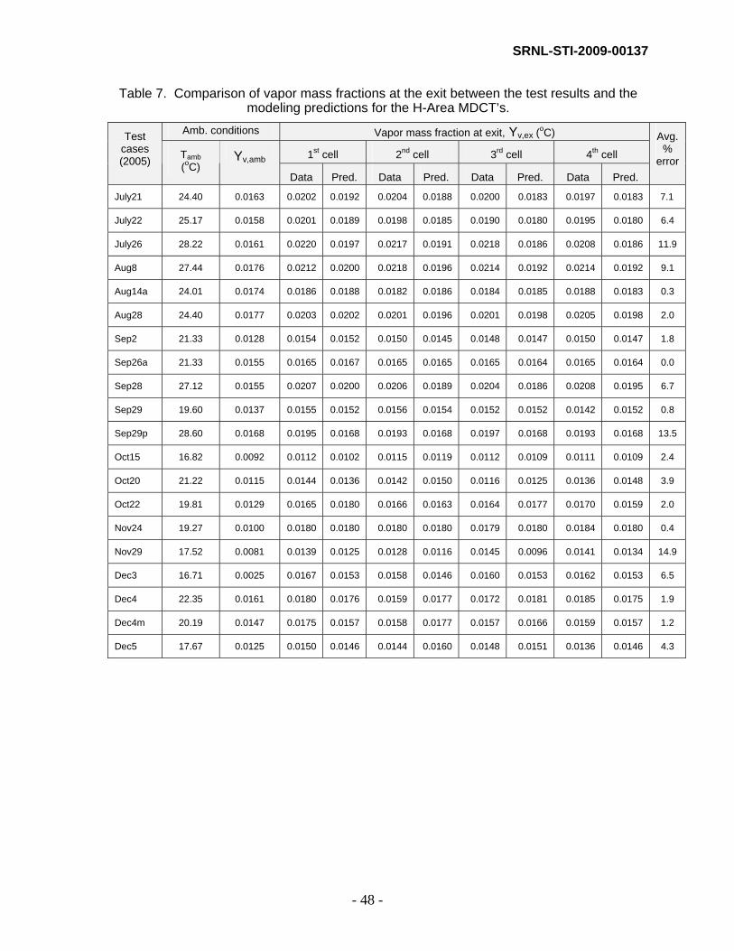
SRNL-STI-2009-00137

- 48 -

Table 7. Comparison of vapor mass fractions at the exit between the test results and the modeling predictions for the H-Area MDCT’s.

Amb. conditions Vapor mass fraction at exit, Yv,ex (oC)

1st cell 2nd cell 3rd cell 4th cell

Test cases (2005) Tamb

(oC) Yv,amb

Data Pred. Data Pred. Data Pred. Data Pred.

Avg.%

error

July21 24.40 0.0163 0.0202 0.0192 0.0204 0.0188 0.0200 0.0183 0.0197 0.0183 7.1

July22 25.17 0.0158 0.0201 0.0189 0.0198 0.0185 0.0190 0.0180 0.0195 0.0180 6.4

July26 28.22 0.0161 0.0220 0.0197 0.0217 0.0191 0.0218 0.0186 0.0208 0.0186 11.9

Aug8 27.44 0.0176 0.0212 0.0200 0.0218 0.0196 0.0214 0.0192 0.0214 0.0192 9.1

Aug14a 24.01 0.0174 0.0186 0.0188 0.0182 0.0186 0.0184 0.0185 0.0188 0.0183 0.3

Aug28 24.40 0.0177 0.0203 0.0202 0.0201 0.0196 0.0201 0.0198 0.0205 0.0198 2.0

Sep2 21.33 0.0128 0.0154 0.0152 0.0150 0.0145 0.0148 0.0147 0.0150 0.0147 1.8

Sep26a 21.33 0.0155 0.0165 0.0167 0.0165 0.0165 0.0165 0.0164 0.0165 0.0164 0.0

Sep28 27.12 0.0155 0.0207 0.0200 0.0206 0.0189 0.0204 0.0186 0.0208 0.0195 6.7

Sep29 19.60 0.0137 0.0155 0.0152 0.0156 0.0154 0.0152 0.0152 0.0142 0.0152 0.8

Sep29p 28.60 0.0168 0.0195 0.0168 0.0193 0.0168 0.0197 0.0168 0.0193 0.0168 13.5

Oct15 16.82 0.0092 0.0112 0.0102 0.0115 0.0119 0.0112 0.0109 0.0111 0.0109 2.4

Oct20 21.22 0.0115 0.0144 0.0136 0.0142 0.0150 0.0116 0.0125 0.0136 0.0148 3.9

Oct22 19.81 0.0129 0.0165 0.0180 0.0166 0.0163 0.0164 0.0177 0.0170 0.0159 2.0

Nov24 19.27 0.0100 0.0180 0.0180 0.0180 0.0180 0.0179 0.0180 0.0184 0.0180 0.4

Nov29 17.52 0.0081 0.0139 0.0125 0.0128 0.0116 0.0145 0.0096 0.0141 0.0134 14.9

Dec3 16.71 0.0025 0.0167 0.0153 0.0158 0.0146 0.0160 0.0153 0.0162 0.0153 6.5

Dec4 22.35 0.0161 0.0180 0.0176 0.0159 0.0177 0.0172 0.0181 0.0185 0.0175 1.9

Dec4m 20.19 0.0147 0.0175 0.0157 0.0158 0.0177 0.0157 0.0166 0.0159 0.0157 1.2

Dec5 17.67 0.0125 0.0150 0.0146 0.0144 0.0160 0.0148 0.0151 0.0136 0.0146 4.3

SRNL-STI-2009-00137

- 49 -

5.0 RESULTS AND DISCUSSIONS

The field test data for the A-Area and H-Area mechanical draft cooling towers were used to benchmark the present simulations. Measurements were taken of the air inlet and exit temperatures, the ambient pressure, the water flow rate and its temperatures at the inlet and outlet. The detailed discussions of the measurement locations were provided in the previous sections. Thirteen sets of the measured data from the A-Area tower and twenty sets of the H-Area test results were compared with the modeling predictions.

Key physical models for turbulence model, evaporative droplet cooling were validated against the literature data. The validated model [14] were applied to the integral benchmarking test against the onsite test results for the A-Area and H-Area cooling towers. Comparison of the predicted and measured exit air temperatures for the A-Area and H-Area cooling towers are made in Fig. 43. The results show that the modeling predictions for the H-Area system are about 10% better than those of the A-Area system because of two potential reasons. One reason is that the model assumes uniform water distributions at the cell inlet, although the test results show that they are not uniform for the ambient and operating conditions (are you referring to the A-Area tower?). The other is probably due to the modeling assumption that an array of the staggered thin-rectangular plates for splitting the water droplets inside each cell has negligible impact on the cell residence time of the ambient air stream to be used for water cooling. Figure 44 compares the predicted and measured vapor mass fractions at the exit for the A-Area and H-Area cooling towers.

The benchmarked model for the A-Area cooling tower was used to the evaluate the impact of wind speed and direction on the air velocity at the exit of the cooling tower. The results indicate that when wind direction is 90 or 270 degrees relative to the plant north, the magnitude of the exit air velocity is only 10 % of the incoming wind speed. For the case with plant-north or plant-south wind direction, the cell exit velocity magnitude will reach a maximum of 34 % of the wind speed. The nondimensional air velocities at the shroud exit, when scaled by the incoming wind speed, collapse to a single curve as shown in Fig. 45. Parametric results for 2, 4, and 8 m/sec wind speeds with various wind directions for the A-Area cooling tower are shown in Tables 8 to 10, respectively.

Figure 46 shows the nondimensional air velocities at the shroud exit as a function of wind direction for three different wind speeds in the H-Area cooling tower. The results show that when the wind direction approaches within 90 or 270 degrees of plant north, the exit air velocity is at a minimum due to the wind shield effect as shown in Fig. 1. Parametric results for 2, 4, and 8 m/sec wind speeds with various wind directions for the H-Area cooling tower are shown in Tables 11 to 13, respectively. Figure 47 shows that the nondimensional air velocities at the shroud exit from the H-Area tower are less sensitive to the wind direction. This is due to a greater inlet flow area and smaller pressure drop in the A-Area cooling tower as compared to the H-Area cooling tower.

SRNL-STI-2009-00137

- 50 -

Measured air exit temperature (deg C)

Pre

dict

edai

rex

itte

mpe

ratu

re(d

egC

)

10 15 20 25 30 3510

15

20

25

30

35

H-Area cooling towerA-Area cooling tower

Figure 43. Comparison of the predicted and measured exit air temperatures for the A-Area

and H-Area cooling towers.

Measured vapor mass fraction

Pre

dict

edva

por

mas

sfr

actio

n

0.005 0.01 0.015 0.02 0.025 0.03

0.005

0.01

0.015

0.02

0.025

0.03

A-Area cooling towerH-Area cooling tower

Figure 44. Comparison of the predicted and measured vapor mass fractions at the exit for

the A-Area and H-Area cooling towers.

SRNL-STI-2009-00137

- 51 -

N

36.3oUoθο

vex

Wind direction, θο

Non-dimensional wind direction

No

n-d

imen

sio

nal

air

exit

velo

city

0 0.2 0.4 0.6 0.8 1 1.2 1.4 1.6 1.8 20

0.1

0.2

0.3

0.4

0.5Wind speed

2 m/sec (A-Area)4 m/sec (A-Area)8 m/sec (A-Area)

(Nondimensional air exit velocity, η = vex/Uo; Nondimensional wind direction, ζ = θo /180o)

Figure 45. Nondimensional air velocities at the shroud exit as a function of wind direction for

three different wind speeds in the A-Area tower.

SRNL-STI-2009-00137

- 52 -

Table 8. Parametric results for a 2 m/sec wind speed with various wind directions for the A-Area cooling tower.

Wind speed (m/sec)

Wind direction (Clockwise angle w.r.t

true north)

Avg. exit vel.

(m/sec)

∆P*

(Pa)

2 0 0.5259 2.7386

2 30 0.3065 1.3267

2 60 0.2064 0.6042

2 90 0.396 2.0678

2 120 0.604 3.2366

2 150 0.6688 3.3762

2 180 0.5373 2.8215

2 210 0.3161 1.4196

2 240 0.2054 0.6099

2 270 0.3906 1.9438

2 300 0.5999 3.0715

2 330 0.6593 3.2601

2 360 0.5255 2.7482

Note:*Difference between area-averaged upstream and downstream pressures of A-Area cooling tower

SRNL-STI-2009-00137

- 53 -


Wind speed (m/sec)


true north)

Avg. exit vel.

(m/sec)

∆P*

(Pa)

4 0 1.0463 11.1044

4 30 0.6025 5.4567

4 60 0.4117 2.3967

4 90 0.7846 8.3673

4 120 1.1958 13.3847

4 150 1.3407 13.4929

4 180 1.0694 11.4903

4 210 0.6268 5.643

4 240 0.3959 2.5589

4 270 0.798 7.7421

4 300 1.2116 12.646

4 330 1.3153 13.4744

4 360 1.0551 11.0535


SRNL-STI-2009-00137

- 54 -


Wind speed (m/sec)


true north)

Avg. exit vel.

(m/sec)

∆P*

(Pa)

8 0 0.2628 44.1814

8 30 0.1500 23.068

8 60 0.1036 10.3504

8 90 0.2014 32.8714

8 120 0.3007 52.6482

8 150 0.3348 54.3577

8 180 0.2678 45.8295

8 210 0.1561 23.811

8 240 0.0993 10.5423

8 270 0.1966 32.4687

8 300 0.3017 50.9955

8 330 0.3312 52.4489

8 360 0.2611 44.3284


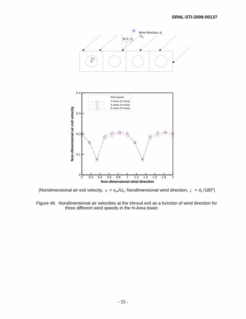
SRNL-STI-2009-00137

- 55 -

N

36.3oUoθο

vex



No

n-d

imen

sio

nal

air

exit

velo

city

0 0.2 0.4 0.6 0.8 1 1.2 1.4 1.6 1.8 20

0.1

0.2

0.3

0.4Wind speed

2 m/sec (H-Area)4 m/sec (H-Area)8 m/sec (H-Area)


Figure 46. Nondimensional air velocities at the shroud exit as a function of wind direction for

three different wind speeds in the H-Area tower.

SRNL-STI-2009-00137

- 56 -

Table 11. Parametric results for a 2 m/sec wind speed with various wind directions in the H-Area cooling tower.

Wind speed

(m/sec)


true north)

Avg. exit vel.

(m/sec)

∆P*

(Pa)

2 0 0.3825 1.3551

2 30 0.3146 0.7552

2 60 0.1416 0.1301

2 90 0.3578 1.0380

2 120 0.3851 1.2220

2 150 0.4038 1.3965

2 180 0.3832 1.1634

2 210 0.3155 0.6535

2 240 0.1439 0.1181

2 270 0.3579 1.1361

2 300 0.3846 1.3686

2 330 0.4033 1.5490

2 360 0.3825 1.3551

Note:*Difference between area-averaged upstream and downstream pressures of cooling tower

SRNL-STI-2009-00137

- 57 -


Wind speed

(m/sec)


true north)

Avg. exit vel.

(m/sec)

∆P*

(Pa)

4 0 0.7961 6.3330

4 30 0.6375 3.8876

4 60 0.3088 0.9486

4 90 0.7438 4.7443

4 120 0.8040 5.8114

4 150 0.8296 6.1010

4 180 0.7994 5.5854

4 210 0.6377 3.4563

4 240 0.3089 0.9062

4 270 0.7444 5.1070

4 300 0.8041 6.5088

4 330 0.8299 6.8331

4 360 0.7961 6.3330


SRNL-STI-2009-00137

- 58 -


Wind speed

(m/sec)


true north)

Avg. exit vel.

(m/sec)

∆P*

(Pa)

8 0 1.6316 27.0904

8 30 1.2560 16.5676

8 60 0.6106 4.3864

8 90 1.5077 21.9085

8 120 1.6504 24.3803

8 150 1.6681 25.0166

8 180 1.6351 24.5042

8 210 1.2556 14.8115

8 240 0.6104 3.9006

8 270 1.5066 23.5050

8 300 1.6499 27.3059

8 330 1.6684 28.0186

8 360 1.6316 27.0904


SRNL-STI-2009-00137

- 59 -

N

36.3oUoθο

vex



No

n-di

men

sio

nala

irex

itve

loci

ty

0 0.2 0.4 0.6 0.8 1 1.2 1.4 1.6 1.8 20

0.1

0.2

0.3

0.4

0.5Wind speed

2 m/sec (A-Area)2 m/sec (H-Area)


Figure 47. Comparison of nondimensional air velocities at the shroud exit at a wind speed

of 2 m/sec for the A-Area and H-Area cooling towers.

SRNL-STI-2009-00137

- 60 -

6.0 CONCLUSIONS AND SUMMARY

A three-dimensional steady-state CFD model was developed for the SRS four-cell MDCT systems in A-Area and H-Area to evaluate the flow patterns and heat transfer characteristics inside the cooling tower during induced draught and wind driven conditions. The CFD model used a standard two-equation turbulence model to capture the turbulent flow behavior of the air inside and outside the tower cells. The model considered a air-vapor mixture that was coupled with water droplet flow, assuming that the vapor phase is always transported by the continuous air phase with no slip velocity. In this work, water droplet flow was considered as discrete phase via a Lagrangian approach for the mass and sensible heat transfer. Simple geometric models were developed to obtain the benchmarking database for verifying the CFD model.

A series of the modeling calculations was performed to investigate the impact of the ambient and operating conditions on flow patterns and heat transfer characteristics inside the cell of the cooling tower. The modeling predictions are in reasonably good agreement with the test results. It was also demonstrated that the CFD method is applicable to the detailed modeling analysis of a cooling tower system.

SRNL-STI-2009-00137

- 61 -

7.0 REFERENCES

1. HOBO Water Temp Pro Logger, www.microdaq.com. 2. FLUENT, 2006, Fluent, Inc., Lebanon, New Hampshire. 3. S. Ergun, 1952, “Fluid through Packed Columns”, Chemical Engineering Progress,

Vol. 18, No. 2, pp. 87. 4. Tech Sales Co. website, “Cooling Tower Drift Eliminators”, www.tech-

sales/Kimre_cooling_tower_drift_eliminators.htm, June 14, 2006. 5. W. P. Jones and P. E. Launder, 1972, “The Prediction of Laminarization with a Two-

Equation Model of Turbulence”, Int. Journal of Heat and Mass Transfer, Vol. 15, pp. 301-314, 1972.

6. P. V. Nielsen, A. Restivo, and J. H. Whitelaw, 1978, “The Velocity Characteristics of Ventilated Rooms”, ASME J. of Fluids Engineering, Vol. 100, pp. 291-298.

7. S. Y. Lee, R. A. Dimenna, R. A. Leishear, D. B. Stefanko, 2008, “Analysis of Turbulent Mixing Jets in a Large Scale Tank”, ASME Journal of Fluids Engineering, Volume 130, Number 1, pp. 011104.

8. W. E. Ranz and W. R. Marshall, Jr., 1952, Part II, Evaporation from Drops”, Chemical Eng. Progress, vol. 48, pp. 173-180.

9. D. P. Kessler and R. A. Greenkorn, Momentum, Heat Mass Transfer Fundamentals, Mercel Dekker, Inc., New York, 1999.

10. S. P. Fisenko, A. A. Brin, and A. I. Petruchik, 2004, “Evaporative Cooling of Water in a Mechanical Draft Cooling Tower”, Int. J. of Heat and Mass Transfer, Vol. 47, pp. 165-177.

11. S. C. Yao and V. E. Schrock, 1976, “Heat and Mass transfer from Freely Falling Drops”, Trans. ASME J. of Heat Transfer, pp. 120-126.

12. S. A. Morsi and A. J. Alexander, 1972, “An Investigation of Particle Trajectories in Two-Phase Flow Systems”, J. of Fluid Mechanics, vol. 55, pp. 193-208.

13. Brentwood Industries, Inc., Pennsylvania, www.brentwoodindustries.com. 14. S. Y. Lee, A. J. Garrett, J. S. Bollinger, and L. D. Koffman, “CFD Modeling Analysis

for Mechanical Draft Cooling Tower”, 2008, ASME 2008 Summer Heat Transfer Conference, HT-2008-56080, Jacksonville, Florida.

CFD Modeling Coolingtower-final2

Documents

Transcript of CFD Modeling Coolingtower-final2