Master Project

Centipede Robot Locomotion

Author:Brian Jimenez

Supervisor:Auke Jan Ikspeert

July 26, 2007

Abstract

This master project introduces a logical evolution of the Salamander Robot de-velopped at Biologically Inspired Robotic Group (BIRG) at Swiss Federal Instituteof Technology of Lausanne (EPFL) and focuses on good locomotion gaits that can beobtained adapting the parameters of the robot.

i

Acknowledgements

Almost two years ago, I decided to move to a foreign country, Switzerland, to havethe opportunity to study in one of the most prestigious technical universities in theworld. Since the beginning, I was fascinated by the swiss working culture and thekindness of the people.

In the first semester, I took one course with professor Auke Jan Ijspeert, Modelsof Biological Sensory-Motor Systems, that shown me the scientist aspect of my ca-reer. Suddenly, I realized that I had the opportunity to develop a project in thebiologically inspired robot context and I decided to take part in this project.In the very first meetings with professor Ijspeert, he proposed me to study the loco-motion of a evolution of the salamander robot: the centipede robot. There was someweeks ago that one article from professor Ijspeert and the BIRG group involved onthe salamander project appeared in Science magazine. To study one of the possibleevolutions of this robot was an honor and a big challenge.

Four months later, I can say I have worked on one of favorite topics I can onlythank professor Ijspeert to bring me this opportunity. I would also thank the peoplewho helped me in this project and was close to me when I much needed: I would liketo thank Yvan Bourquin to answer all my questions about Webots platform, withouthis help I would be still debugging code. To professor Auke Jan Ijspeert for helpingme during this project and always giving me good ideas and invaluable orientation.To my very special friends in Switzerland during this year: Margarida, Risto, Javier,Myriam, Natalia, Cristina because they were always listening to me without condi-tions (and I have to admit that sometimes was a heavy work). To my friends fromSpain: Paula and Neus, they were always at the other side waiting for my boringspeeches. To my family because they were working hard to bring me the opportunityto stay here in this moment. This last year I have lived an invaluable experience. Iwill miss you a lot. Thanks very much for being there and let me learn a lot of things.

Lausanne, July 26, 2007

ii

Contents

Abstract i

Acknowledgements ii

List of Tables v

List of Figures vi

1 Introduction 11.1 State of the Art . . . . . . . . . . . . . . . . . . . . . . . . . . . . . . 2

1.1.1 WhegsTMrobot . . . . . . . . . . . . . . . . . . . . . . . . . . 21.1.2 RHex robot . . . . . . . . . . . . . . . . . . . . . . . . . . . . 21.1.3 Salamander robot . . . . . . . . . . . . . . . . . . . . . . . . . 3

1.2 Objectives . . . . . . . . . . . . . . . . . . . . . . . . . . . . . . . . . 41.3 Tools . . . . . . . . . . . . . . . . . . . . . . . . . . . . . . . . . . . . 4

1.3.1 WebotsTM . . . . . . . . . . . . . . . . . . . . . . . . . . . . . 41.3.2 Art of Illusion . . . . . . . . . . . . . . . . . . . . . . . . . . . 51.3.3 CentipedeScript . . . . . . . . . . . . . . . . . . . . . . . . . . 5

1.4 Structure of the report . . . . . . . . . . . . . . . . . . . . . . . . . . 5

2 Architecture 72.1 Body module . . . . . . . . . . . . . . . . . . . . . . . . . . . . . . . 72.2 Head module . . . . . . . . . . . . . . . . . . . . . . . . . . . . . . . 72.3 Limbs module . . . . . . . . . . . . . . . . . . . . . . . . . . . . . . . 92.4 Centipede robot model . . . . . . . . . . . . . . . . . . . . . . . . . . 92.5 Beyond nature . . . . . . . . . . . . . . . . . . . . . . . . . . . . . . . 10

3 CentipedeScript 123.1 How to build a new robot model? . . . . . . . . . . . . . . . . . . . . 133.2 How to configure the robot model with CentipedeScript? . . . . . . . 133.3 How to extend CentipedeScript? . . . . . . . . . . . . . . . . . . . . . 14

iii

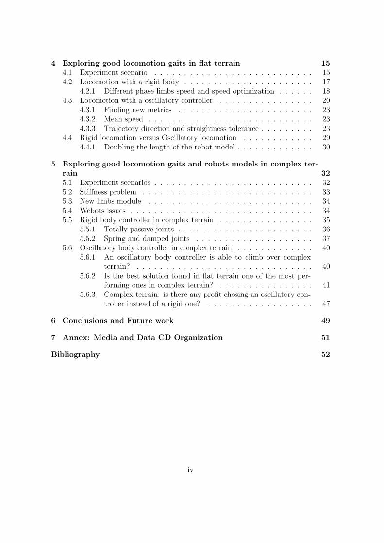
4 Exploring good locomotion gaits in flat terrain 154.1 Experiment scenario . . . . . . . . . . . . . . . . . . . . . . . . . . . 154.2 Locomotion with a rigid body . . . . . . . . . . . . . . . . . . . . . . 17

4.2.1 Different phase limbs speed and speed optimization . . . . . . 184.3 Locomotion with a oscillatory controller . . . . . . . . . . . . . . . . 20

4.3.1 Finding new metrics . . . . . . . . . . . . . . . . . . . . . . . 234.3.2 Mean speed . . . . . . . . . . . . . . . . . . . . . . . . . . . . 234.3.3 Trajectory direction and straightness tolerance . . . . . . . . . 23

4.4 Rigid locomotion versus Oscillatory locomotion . . . . . . . . . . . . 294.4.1 Doubling the length of the robot model . . . . . . . . . . . . . 30

5 Exploring good locomotion gaits and robots models in complex ter-rain 325.1 Experiment scenarios . . . . . . . . . . . . . . . . . . . . . . . . . . . 325.2 Stiffness problem . . . . . . . . . . . . . . . . . . . . . . . . . . . . . 335.3 New limbs module . . . . . . . . . . . . . . . . . . . . . . . . . . . . 345.4 Webots issues . . . . . . . . . . . . . . . . . . . . . . . . . . . . . . . 345.5 Rigid body controller in complex terrain . . . . . . . . . . . . . . . . 35

5.5.1 Totally passive joints . . . . . . . . . . . . . . . . . . . . . . . 365.5.2 Spring and damped joints . . . . . . . . . . . . . . . . . . . . 37

5.6 Oscillatory body controller in complex terrain . . . . . . . . . . . . . 405.6.1 An oscillatory body controller is able to climb over complex

terrain? . . . . . . . . . . . . . . . . . . . . . . . . . . . . . . 405.6.2 Is the best solution found in flat terrain one of the most per-

forming ones in complex terrain? . . . . . . . . . . . . . . . . 415.6.3 Complex terrain: is there any profit chosing an oscillatory con-

troller instead of a rigid one? . . . . . . . . . . . . . . . . . . 47

6 Conclusions and Future work 49

7 Annex: Media and Data CD Organization 51

Bibliography 52

iv

List of Tables

2.1 Dimensions of body module. . . . . . . . . . . . . . . . . . . . . . . . 72.2 Dimensions of limbs module. . . . . . . . . . . . . . . . . . . . . . . . 9

5.1 Hill’s measures . . . . . . . . . . . . . . . . . . . . . . . . . . . . . . 325.2 Triangle mesh rendering errors . . . . . . . . . . . . . . . . . . . . . . 355.3 Travelled distance with passive joints . . . . . . . . . . . . . . . . . . 365.4 Travelled distance with passive joints and an extra tail module. . . . 375.5 Travelled distance (m) depending on ω and µ in scenario A. . . . . . 395.6 Travelled distance mean (µ), standard deviation (σ) and maximum value. 425.7 Complex terrain test parameters. . . . . . . . . . . . . . . . . . . . . 475.8 Covered distance (m) . . . . . . . . . . . . . . . . . . . . . . . . . . . 47

v

List of Figures

1.1 Amphibot II . . . . . . . . . . . . . . . . . . . . . . . . . . . . . . . . 11.2 WhegsTMII robot. . . . . . . . . . . . . . . . . . . . . . . . . . . . . . 21.3 RHex cockroach robot. . . . . . . . . . . . . . . . . . . . . . . . . . . 31.4 Salamander robot. . . . . . . . . . . . . . . . . . . . . . . . . . . . . 31.5 Webots representation of the 16-legs centipede robot. . . . . . . . . . 41.6 Art of Illusion screenshot modelling a hill object. . . . . . . . . . . . 5

2.1 Webots representation of the body module and real module. . . . . . 82.2 Webots representation of the head module. . . . . . . . . . . . . . . . 82.3 Webots representation of the limbs module and real module. . . . . . 92.4 Proposed architectures . . . . . . . . . . . . . . . . . . . . . . . . . . 102.5 Section schema of the scolopendra heros. Image reprinted from [2]. . . 11

3.1 CentipedeScript GUI. . . . . . . . . . . . . . . . . . . . . . . . . . . . 123.2 Different architectures created with CentipedeScript. . . . . . . . . . 14

4.1 Ground contact points in scolopendra heros locomotion over time. Im-age reprinted from [2]. . . . . . . . . . . . . . . . . . . . . . . . . . . 16

4.2 Flat terrain example. . . . . . . . . . . . . . . . . . . . . . . . . . . . 164.3 Speed obtained changing the phase angle between legs. . . . . . . . . 184.4 Zero phase difference angle with a rigid body controller. . . . . . . . . 194.5 Mean Phase Bias Speed depending on Ak and ∆ϕ. . . . . . . . . . . . 224.6 Motion obtained with the maximum found in simulations. . . . . . . 224.7 Mean speed versus amplitude and body and limbs difference phase

angle. Each subgraph represents a modules phase angle step of π4

witha frequency of 0.25Hz. . . . . . . . . . . . . . . . . . . . . . . . . . . 24

4.8 Mean speed versus amplitude and body and limbs difference phaseangle. Each subgraph represents a modules phase angle step of π

4with

a frequency of 0.5Hz. . . . . . . . . . . . . . . . . . . . . . . . . . . . 254.9 Mean speed versus amplitude and body and limbs difference phase

angle. Each subgraph represents a modules phase angle step of π4

witha frequency of 0.75Hz. . . . . . . . . . . . . . . . . . . . . . . . . . . 26

vi

4.10 Mean speed versus amplitude and body and limbs difference phaseangle. Each subgraph represents a modules phase angle step of π

4with

a frequency of 1.0Hz. . . . . . . . . . . . . . . . . . . . . . . . . . . . 274.11 Best solution locomotion behaviour found. . . . . . . . . . . . . . . . 284.12 Straightness tolerance . . . . . . . . . . . . . . . . . . . . . . . . . . . 284.13 Mean Speed examples with frequency equal to 1.0Hz and corrected by

an error of ε = 10%. . . . . . . . . . . . . . . . . . . . . . . . . . . . 294.14 The 32-legs centipede robot. . . . . . . . . . . . . . . . . . . . . . . . 304.15 16-legs robot speed versus 32-legs robot speed. . . . . . . . . . . . . . 31

5.1 Complex terrain scenarios: (a) 14.2% slope, (b) 16.4% slope, (c) 22.3%slope. . . . . . . . . . . . . . . . . . . . . . . . . . . . . . . . . . . . . 33

5.2 The head is blocked and the limbs can not touch the ground. . . . . . 335.3 New limbs module. The red line represents the new y-axis rotation DOF. 345.4 Bounding box models: (a)cylinder and (b)box. . . . . . . . . . . . . . 355.5 (a) not enough triangle density, (b)sufficient triangle density. . . . . . 365.6 (a) Head stuck (b) Tail stuck. . . . . . . . . . . . . . . . . . . . . . . 375.7 (a) 16.4% slope. Red arrow points to the extra module. (b) Final

position of the extra module added model in a 22.3% slope scenario.The robot is not able to climb. . . . . . . . . . . . . . . . . . . . . . . 38

5.8 Simple mass-spring-damper system. Reprinted from [13] with permission. 385.9 Model explosion in Webots simulation. . . . . . . . . . . . . . . . . . 395.10 The red line delimits the obstacles area. . . . . . . . . . . . . . . . . 425.11 Complex terrain scenarios: (a) 14.2% slope, (b) 16.4% slope, (c) 22.3%

slope. . . . . . . . . . . . . . . . . . . . . . . . . . . . . . . . . . . . . 435.12 Travelled distance in scenario A with oscillatory controller. . . . . . . 445.13 Travelled distance in scenario B with oscillatory controller. . . . . . . 455.14 Travelled distance in scenario C with oscillatory controller. . . . . . . 46

vii

Chapter 1

Introduction

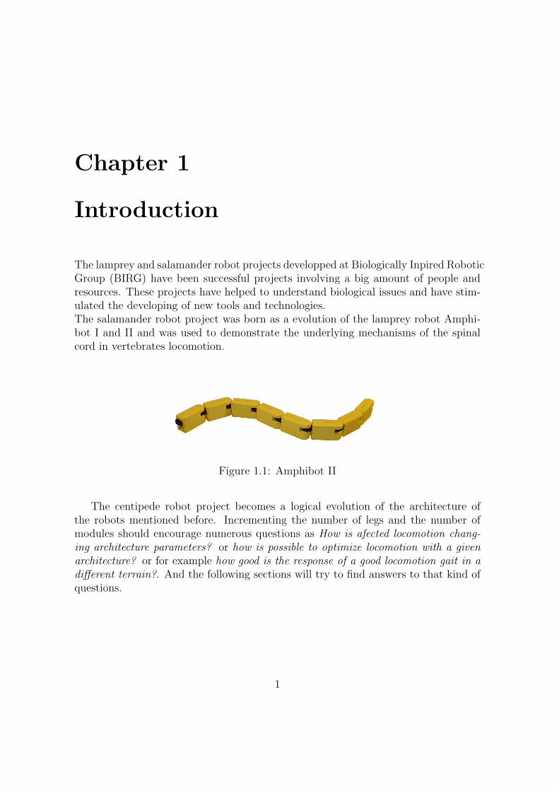
The lamprey and salamander robot projects developped at Biologically Inpired RoboticGroup (BIRG) have been successful projects involving a big amount of people andresources. These projects have helped to understand biological issues and have stim-ulated the developing of new tools and technologies.The salamander robot project was born as a evolution of the lamprey robot Amphi-bot I and II and was used to demonstrate the underlying mechanisms of the spinalcord in vertebrates locomotion.

Figure 1.1: Amphibot II

The centipede robot project becomes a logical evolution of the architecture ofthe robots mentioned before. Incrementing the number of legs and the number ofmodules should encourage numerous questions as How is afected locomotion chang-ing architecture parameters? or how is possible to optimize locomotion with a givenarchitecture? or for example how good is the response of a good locomotion gait in adifferent terrain?. And the following sections will try to find answers to that kind ofquestions.

1

(a) (b)

Figure 1.2: WhegsTMII robot.

1.1 State of the Art

This section presents some of the newest developments in robots models that areproximal to the centipede robot model presented in this project. The robot modelpresented in this project has been inspired in some of these robots and some goodsolutions and ideas to similar problems have been considered and incorporated to ourmodel.

1.1.1 WhegsTMrobot

WhegsTMrobot is an interesting robotic project developed in the Biologically InspiredRobotic Group of the Case Western Reserve University, USA. Whegs I and II, [11], [1]and [3], are hexapod robots with the particularity that incorpores wheel-legs insteadof traditioanl legs. Salamander robot inherits the concept of rotational legs from theWhegs robot. Whegs II incorporates a body joint that allows the robot to climbobstacles.

1.1.2 RHex robot

RHex robot has been developed at PolyPEDAL Laboratory of the Department ofIntegrative Biology in the Berkeley University of California. RHex is a cockroachinspired robot and has been used to study insect locomotion and mechanical aspectsof legged locomotion. In [12] and [7] articles, RHex appears as a model solution toa universal problem that is legged comotion and the conversion of solutions betweeninsects and vertebrates.

2

Figure 1.3: RHex cockroach robot.

(a) (b)

Figure 1.4: Salamander robot.

1.1.3 Salamander robot

At the introduction of this chapter was firstly mentioned that the centipede robotappears as a obvious evolution of the salamander robot developed at BiologicallyInpired Robotic Group in the Swiss Federal Institute of Technology of Lausanne(EPFL). Salamader robot was driven by a Central Pattern Generator (CPG) con-troller and has different locomotion gaits depending on the environment (swimmingor walking). Salamander robot, [4], [5] and [6], investigates the transition from swim-ming to walking during vertebrate evolution. The basic centipede robot modules arebased on the salamander robot modules.

3

1.2 Objectives

The main objective of this project is to explore the possibility of adding and extendingthe actual salamander robot increasing the number of limbs of the robot. Differentarchitectures based on a centipede-shape robot have to be proposed and studied.Then, the chosen architecture locomotion has to be tested on different scenarios, flatterrain and complex terrain. In flat terrain the project has to focus on the goodlocomotion gaits and in complex terrain the robot model has to be validated and,possibly, changed according to problems and restrictions that can appear on thesecomplex terrain scenarios.

1.3 Tools

In this section the tools used during this project will be presented.

1.3.1 WebotsTM

WebotsTMplatform from Cyberbotics is a fast prototyping environment for program-ming, modelling and testing mobile robots. The main reasons to have chosen Webotsas a preferred platform are:

Figure 1.5: Webots representation of the 16-legs centipede robot.

• Use of the standard VRML language to define the robot and world models in3D.

• Total control over the physics of the simulated world and robot model.

4

• Use of the capabilities of the real hardware to run the simulations as fast aspossible (multiple times the real speed).

1.3.2 Art of Illusion

Art of Illusion (AOI) is a 3D modelling tool written in Java, cross-platform and hasbeen released under General Public License (GPL). Art of Illusion tool has beenused in this project to model the complex terrain scenario for the complex terrainlocomotion experiments.

Figure 1.6: Art of Illusion screenshot modelling a hill object.

1.3.3 CentipedeScript

Besides the use of Webots and AOI, a script has been developed to automate theworld creation and fast selecting the attributes of the robot. For further informationlook up at Chapter 3.

1.4 Structure of the report

The following sections of the report are organized as:

5

Chapter 2 describes the centipede robot architecture and presents the modules in-volved in the construction of the robot model.

Chapter 3 presents the custom script to configure and build the centipede robotmodel.

Chapter 4 explains the experiments and the results obtained finding good loco-motion gaits in a flat terrain scenario.

Chapter 5 explains the experiments and the results obtained finding good loco-motion gaits in complex terrain scenarios.

6

Chapter 2

Architecture

The proposed robot architecture is based on the real hardware developped for theSalamander robot. In the following sections, an exhaustive description of each modulewill be given.

2.1 Body module

The body module incorpores a servo motor on the front (curved part) and an attachingpoint at the back. This servo introduces a new degree of freedom in the horizontalplane with an amplitude of 130. The dimensions are detailed at table 2.1

Table 2.1: Dimensions of body module.

Dimensions (cm)Height 5.6Width 3.8Deep 9.5

2.2 Head module

The head module is a normal body module, but with two CCD cameras on the top-front of the module. This module is added to the model to include some visionfeedback on the robot controller in the future.

7

(a) (b)

Figure 2.1: Webots representation of the body module and real module.

Figure 2.2: Webots representation of the head module.

8

(a) (b)

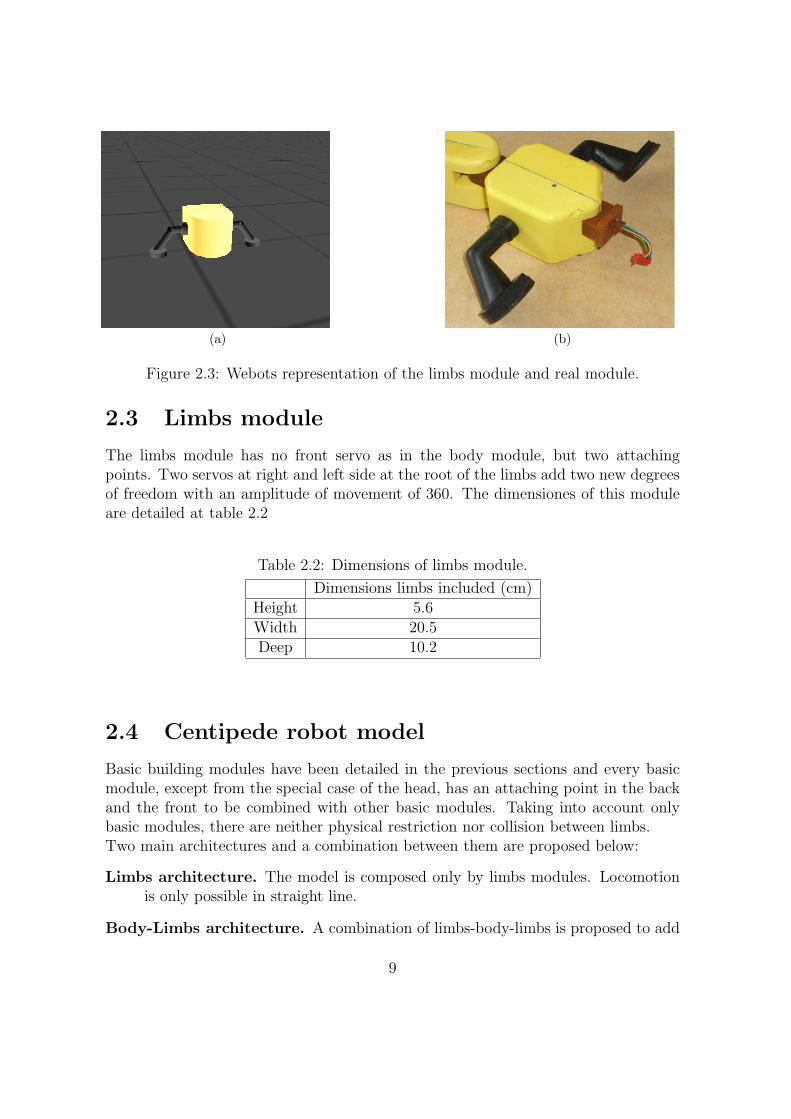
Figure 2.3: Webots representation of the limbs module and real module.

2.3 Limbs module

The limbs module has no front servo as in the body module, but two attachingpoints. Two servos at right and left side at the root of the limbs add two new degreesof freedom with an amplitude of movement of 360. The dimensiones of this moduleare detailed at table 2.2

Table 2.2: Dimensions of limbs module.

Dimensions limbs included (cm)Height 5.6Width 20.5Deep 10.2

2.4 Centipede robot model

Basic building modules have been detailed in the previous sections and every basicmodule, except from the special case of the head, has an attaching point in the backand the front to be combined with other basic modules. Taking into account onlybasic modules, there are neither physical restriction nor collision between limbs.Two main architectures and a combination between them are proposed below:

Limbs architecture. The model is composed only by limbs modules. Locomotionis only possible in straight line.

Body-Limbs architecture. A combination of limbs-body-limbs is proposed to add

9

(a) Only Limbs (b) Limb-body-limb (c) Mixed

Figure 2.4: Proposed architectures

the possibility to oscillate (body servos) to the model to help locomotion andlet the model changing direction.

Mixed architecture. A combination of limbs-body-limbs with subsections com-posed only by limbs modules.

Figure 2.4 shows a schema of the architectures mentioned before.

2.5 Beyond nature

This work is without question inspired by real centipedes and a comparison betweenthe centipede robot model and the animal is inevitable. So, the most importantstructural differences are:

• Number of segments. In nature, centipede have between 15 and 173 segmentsaproximately. The number of modules in the robot model is not fixed, but itwill depend on the architecture and due to bigger size of the modules on thecentipede robot, it will not have as many modules as segments on the nature.

• One segment, two limbs. In nature, each segment has two limbs in each side.Taking into account limbs modules’ restrictions (no possibility of oscillation inthe xz plane), it is necessary to combine limb-body-limb modules. To sum up,in the robot model there are modules without limbs.

• Segment size. In the robot model, each kind of segment has a constant size,whereas in nature the segment size is not constant.

• Limbs. In nature, real limbs have an up and down motion, whereas in theactual robot model, limbs have a rotation motion in the xy plane.

10

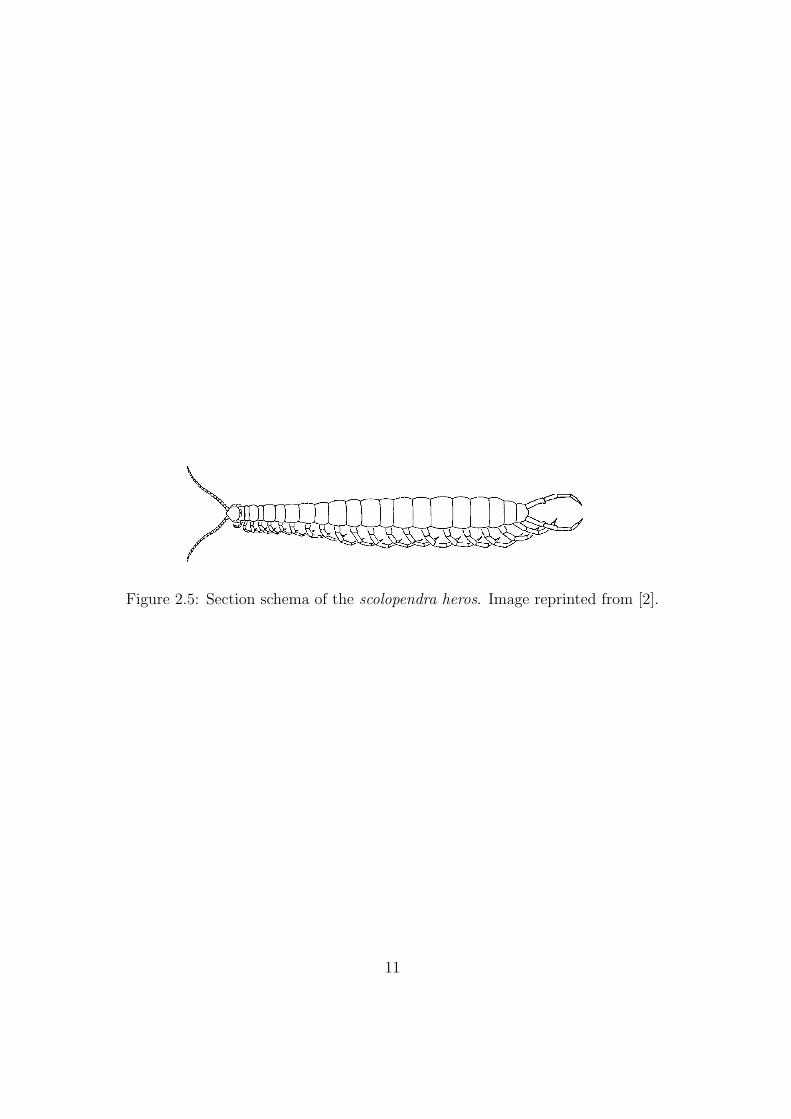
Figure 2.5: Section schema of the scolopendra heros. Image reprinted from [2].

11

Chapter 3

CentipedeScript

CentipedeScript is the name of the application developped in the scope of thisproject for fast building new centipede robot models compatibles with Webots soft-ware. This application has been written in C++ and using Trolltech c© Qt librariesas a cross-platform application capable of being recompiled in most Unix, Windowsand MacOS platforms. Figure 3.1 shows a screenshot of the application.

Figure 3.1: CentipedeScript GUI.

CentipedeScript application is based on the original salamander robot scriptwritten by Yvan Bourquin in the salamader robot project scope.

12

3.1 How to build a new robot model?

To build a new centipede robot model four simple steps:

1. Select a robot module in the Robot Modules frame and click to the button Add toadd the selected module to the robot model. Every module has a representativeimage in the right side of the Robot Modules frame. It is mandatory to select ahead module as a first module of the robot model.

2. Every module has only one-letter shortening and it appears when a module isadded to the robot model in the Actual Configuration frame. Modules can beadded and removed dinamically using the Add and the Cross buttons.

3. Select the scenario in the combo-box from the Scenario frame.

4. Click to Generate and select the location of the output world .wbt file.

3.2 How to configure the robot model with Cen-

tipedeScript?

Appart from the possibilities of selecting several modules, CentipedeScript can beconfigured from a file called centipede.conf. This file has to be found in the samedirectory that the executable. The following parameters can be tuned:

• Dimensions. Femur, tibia and foot dimensions and parameters can be changed.For example, femur length, femur radius and tibia angle variables.

• Physics. According to Webots physics parameters as density, coulomb friction,max speed and mass for example can be configured.

• Additional robots. An extra fly robot can be activated.

• Environment. In this section the dimensions of the aquarium (in case that anaquarium scenario had been selected) can be tuned and even the water level.

• Start position. The start position of the robot can be selected manually.

13

(a) (b) (c)

Figure 3.2: Different architectures created with CentipedeScript.

3.3 How to extend CentipedeScript?

It is possible to extend the original CentipedeScript modules with new ones, but arecompilation of the source code will be required. The steps to extend the Cen-tipedeScript application with new modules are detailed below:

• Add a new entry in the centipedescript.conf configuration file. The file for-mat is

〈 Module Name; Abbrevation; Image Path 〉.

This information is required by the main executable.

• Modify the function isLeg( QString s ) in the source code filecentipescriptv2.cpp to take into account if the new module has limbs or not.

• Create a new function in the source code file centipescriptv2.cpp with theformat

void CentipedeScript::function name( QTextStream *t )

and modify the function void CentipedeScript::generate( QTextStream *t)

according to.

14

Chapter 4

Exploring good locomotion gaits inflat terrain

In this chapter, several locomotion controllers for the centipede robot model willbe explored. First of all, one scenarios will be defined: flat terrain. Then, a fixedarchitecture will be tested in this scenario. This architecture will be a limb-body-limbmodel composed by eight limbs modules, seven body modules and one head module.The advantage of using this architecture is obvious: it is possible to write controllerswith the possibility of changing direction thanks to the extra degree of freedom addedby the body modules. The number of modules is not trivial to be explained, but thereare three main reasons:

1. Eight limbs or more. Less limbs will turn the centipede model in an hexapod,well-known model and tested and studied many times.

2. Aliasing. A small limbs number could entail an aliasing effect when the bodymodel oscillates with a traveling wave from the head to the tail.

3. Too many modules. A big number of modules will increase enourmously thetotal length of the robot without a clear application. As a direct consequence,simulations will take more time due to the increase of modules to be taken intoaccount in physics calculations.

Moreover, in real scolopendra heros locomotion, only a few number of limbs are touch-ing the ground at the time as shown in figure 4.1.So it seems reasonable to have an initial number of limbs of sixteen. Figure 1.5represents the experimental robot model in Webots.

4.1 Experiment scenario

First of all, it is important to define and build the scenario where the experimentswill take place.

15

Figure 4.1: Ground contact points in scolopendra heros locomotion over time. Imagereprinted from [2].

Flat terrain is a 100x100 meters horizontal plane big enough to be able to run thesimulations without having the noise due to have reached the limits of the scenario.Figure 4.2 shows this scenario.

Figure 4.2: Flat terrain example.

16

4.2 Locomotion with a rigid body

A limbs controller was written and the servos from the body modules were fixed toavoid any motion. Equations 4.1 and 4.2 give at each simulation timestep the angleof the servo that controls the limb i in the right and left sides respectively (ϕright andϕleft).

ϕright = ω · t + φr + φ · i (4.1)

ϕleft = ω · t + φl + φ · i (4.2)

Where ω is the angular speed, t the timestep, φr and φl the initial phase angleof right and left limbs respectively and φ the phase angle between limbs of the sameside. All the units are in SI units.

To obtain the results of the graph from Figure 4.3 the parameters of the simulationwere:

• Simulation time of 20 seconds.

• Phase angle between limbs parameter searching interval from −π to π with astep of π

16.

• The variables φr and φl are fixed to π2

and 3π2

due to building characteristicsand a constant phase angle difference between both sides of π radians.

• Frequency (angular speed ω) search of 0.25, 0.5, 0.75 and 1.0 Hz.

• Repetitions of the experiment equal to five.

• Speed is integrated at each timestep as a continuous speed and not as a meanspeed.

Analyzing the data obtained from the experiment, it is possible to draw the followingconclusions:

1. Speed is directly proportional to the frequency.

2. Speed is stable except in the interval [−π4

, π4].

3. Locomotion is (quite near) in forward straight line.

So, the question to be answered is what is happening in that interval? Actually, itwas a expected behaviour because the center of the interval [−π

4, π

4] is the zero phase

angle. When the difference of phase angle between limbs of the same side is zero, all

17

the limbs from the right and left side are in a phase difference of |φr − φl| equal toπ radians. Then, the robot is trying to get up from the ground in a reiterate way asshown in Figure 4.4. The rest of the valours of the interval are less worse than thezero phase angle but useless.

Another good observation is that speed is proportional to frequency, but highfrequencies on the real salamander robot were the cause of slipping between the robotand the ground. Slipping is not desirable because can introduce error in trajectorycalculation, so there is a theoretical top-valour for the frequency that most of timeshas to be found empirically working with real hardware. In this document, the 1Hzfrequency is considered the top-level valour.

Figure 4.3: Speed obtained changing the phase angle between legs.

4.2.1 Different phase limbs speed and speed optimization

As shown in [5], increasing the time that the limb spends on the ground and, in conse-quence, increasing the fly-speed of the limb (the time that the limb is not contactingthe ground) affects the global speed of the robot increasing it. It is possible to apply

18

(a) (b)

(c) (d)

(e) (f)

(g) (h)

Figure 4.4: Zero phase difference angle with a rigid body controller.

19

the same concept on the centipede robot, but it increases enormoursly the computa-tion time of the simulation because for each limb and timestep an angle check has tobe done. This angle check is a comparison between the actual limb rotational angleand the angles Θ1 and Θ2 that are the starting and ending ground touching for thelimbs. This computation takes a long time because is a comparison between floatsand a float module is required to be computed.Because of the big similarities between salamander robot and centipede robot models,the optimization before is recommended, but not tested in this document.

4.3 Locomotion with a oscillatory controller

In [2] the scolopendra heros centipede locomotion is studied to demonstrate Manton’smodels, [8], [9] and [10]. Manton considered a straight rigid body as an optimal forefficient forward locomotion and in [2] and after the study of the electromyograms(EMGs) signals capted in the muscle activity of the scolopendra heros, they concludethat lateral muscles are not resistive to lateral bending, but promoting it. Is the goalof this section to study if the lateral bending and the propagation of a traveling waveamong the body length can optimize the forward locomotion.

Again, the limb controller is based on equations 4.1 and 4.2. The body modulesservos are controlled by the expression 4.3.

f(k) = Ak sin(ω · t + ϕ + ∆ϕ · k) (4.3)

In Equation 4.3, ω represents the angular speed, t the timestep, ϕ is the phaseangle difference between the limbs and body, ∆ϕ is the phase angle difference be-tween the body modules and Ak is the amplitude of the servo, a valour in the interval[0.0, 1.1] that are the physical limits of the body servo. Again, all parameters areexpressed in SI units.

Again, the goal is to find good valours for the variables of equation 4.3, speciallyfor ϕ, ∆ϕ and Ak. The parameters of the simulations were:

• Simulation time of 20 seconds.

• Phase angle difference between limbs fixed to π2, a valour found in previous

section.

• Limbs controller parameters rest with the same valour as in the previous section.

• Frequency (angular speed ω) search of 0.25, 0.5, 0.75 and 1.0 Hz.

20

• Phase angle between limbs and body (ϕ) parameter searching interval from −πto π with a step of π

4.

• Phase angle between body modules (∆ϕ) parameter searching interval from −πto π with a step of π

4.

• Amplitude of the body servo (Ak) parameter searching interval from 0.1 to 1.0with a granularity of 0.05.

• Speed is integrated at each timestep as a continuous speed and is also savedmean speed, total distance traveled and angle between origin and final position.

A simulation at each searching frequency (0.25,0.5,0.75 and 1.0 Hz) has been exe-cuted. Due to large simulation times (over 12 hours of exhaustive computation time),each simulated has been executed only once.

Figure 4.5 shows the results from the simulations. Subgraphs (a), (b), (c) and(d) represent the variation of speed with frequencies 0.25, 0.5, 0.75 and 1.0Hz respec-tively. The speed in z axis is the mean between the eight different possibilities in thephase angle difference between body and limbs, ϕ, search space (from −π to π witha step of π

4).

Interpreting the results, some observations can be made:

• Again, it seems that speed increases with frequency. The same observation asin the rigid body can be applied in this case.

• For different phase angle difference between limbs and body, ϕ, the speed valuesare very similar and grow in the same proportion.

• There seems to exist a maximum point in the function without being functionof the frequency or ϕ.

If the simulation is rerun with the values of the maximum found, the motionrepresented in Figure 4.6. This motion seems not to be an optimal one as the topvalour of the speed shows. In fact, the locomotion found is a bizarre case where thedifference phase angle between limbs is set to zero and different valours for amplitudemake the robot bend in a coordinate way to reach even a circular shape in the worsecase. This bending causes high-peaks in the instant speed and points to a new changeof quantitative and qualitative metric to found good locomotion gaits in oscillatorymode.

21

(a) (b)

(c) (d)

Figure 4.5: Mean Phase Bias Speed depending on Ak and ∆ϕ.

(a) (b) (c) (d)

(e) (f) (g) (h)

Figure 4.6: Motion obtained with the maximum found in simulations.

22

4.3.1 Finding new metrics

Total distance traveled, initial and final positions, angle between initial and finalpositions and mean speed are calculated at the end of each simulation. It seemsreasonable to emphasize mean speed as a quantitative metric and angle difference asa qualitative metric of the found behaviour.

4.3.2 Mean speed

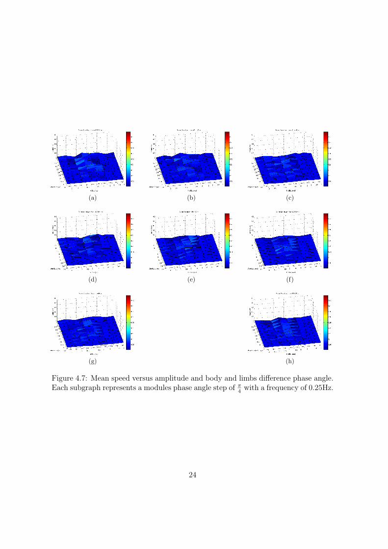
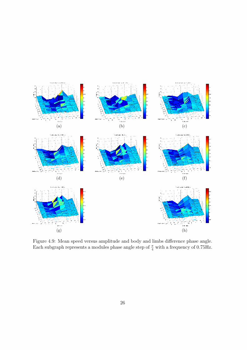
Mean speed as traveled distance are good metrics to quantify the quality of thelocomotion gait found. Figures 4.7, 4.8, 4.9 and 4.10 show with equal scale meanspeed versus amplitude and body and limbs difference phase angle for each bias stepand frequencies of 0.25, 0.5, 0.75 and 1.0 Hz respectively.Analyzing the data, several observations can be made again:

• Again, speed seems to be proportional to frequency.

• Speed function shape depending on amplitude and difference phase angle be-tween limbs and body seems to be less chaotic and more stable for positivevalues of body modules phase angle.

• Best solutions have been found at high frequencies.

If the best solution found is rerun (Ak = 1.0, ∆ϕ = −π2

and ϕ = 0), a locomotionbehaviour as shown in the Figure 4.11 can be observed.These parameters develop a well-defined traveling wave along the robot body andthe length of this traveling wave is exactly the 2

3length of the body. In fact, ϕ = 0

also contributes to speed up the robot avoiding any interference between the travelingwave and the limbs rotation.Next section will try to investigate if it is still possible to optimize the quality of thebest solution found.

4.3.3 Trajectory direction and straightness tolerance

If it is important the straightness of the trajectory, the angle between the initialposition and the final position has to be proximal to 90 (π

2rad). For example, it will

be interesting to filter the best solutions by this angle. The filter could follow theexpression 4.4.

α ∈ [π − ε

2,π + ε

2] (4.4)

Variable ε can be interpreted as the tolerance that can be assumed. In Figure 4.12can be appreciated a tolerance error of ϕ = 4% and Θ = 12.5%.

23

(a) (b) (c)

(d) (e) (f)

(g) (h)

Figure 4.7: Mean speed versus amplitude and body and limbs difference phase angle.Each subgraph represents a modules phase angle step of π

4with a frequency of 0.25Hz.

24

(a) (b) (c)

(d) (e) (f)

(g) (h)

Figure 4.8: Mean speed versus amplitude and body and limbs difference phase angle.Each subgraph represents a modules phase angle step of π

4with a frequency of 0.5Hz.

25

(a) (b) (c)

(d) (e) (f)

(g) (h)

Figure 4.9: Mean speed versus amplitude and body and limbs difference phase angle.Each subgraph represents a modules phase angle step of π

4with a frequency of 0.75Hz.

26

(a) (b) (c)

(d) (e) (f)

(g) (h)

Figure 4.10: Mean speed versus amplitude and body and limbs difference phase angle.Each subgraph represents a modules phase angle step of π

4with a frequency of 1.0Hz.

27

(a)

(b)

(c)

(d)

Figure 4.11: Best solution locomotion behaviour found.

Figure 4.12: Straightness tolerance

28

(a) (b)

(c) (d)

Figure 4.13: Mean Speed examples with frequency equal to 1.0Hz and corrected byan error of ε = 10%.

Figure 4.13 shows two examples of the mean speed corrected with an error ε = 10%.The results that are outside the error cone are set to zero in (b) and (d) subgraphs.It seems to be a pattern in the corrected results, but it depends on the toleranceerror chosen and in the phase angle difference between body modules (∆ϕ) negativeor proximal to zero.

4.4 Rigid locomotion versus Oscillatory locomo-

tion

As was mentioned in the last section, the goal was to demostrate if the lateral bendingin the centipede robot model was able to optimize the forward locomotion. If the bestsolutions found in rigid and oscillatory locomotion in terms of speed are compared,it seems that the oscillatory controller is improving the speed over a 80% (0.25 m/s

29

in rigid body locomotion versus 0.45 m/s in oscillatory locomotion). It is possible tocompare both visually on the BIRG website at url.

4.4.1 Doubling the length of the robot model

One interesting question that can be asked is if we double the length, how good willbe the best solution found in a 16-legs centipede robot?.

Figure 4.14: The 32-legs centipede robot.

The new model has been built and the speed from the 16-legs and the 32-legs havebeen compared for ten simulations. Figure 4.15 shows the speeds obtained. As it canbe observed, speeds obtained for both robot models are quite similar, so it seemsreasonable to conclude that doubling the length of the robot the speed is preserved.

30

Figure 4.15: 16-legs robot speed versus 32-legs robot speed.

31

Chapter 5

Exploring good locomotion gaitsand robots models in complexterrain

In this chapter, the experimental results obtained in last chapter will be used to findgood robot models and good locomotion gaits in complex terrain. In the first section,complex terrain scenarios will be proposed. Then, the problem of the stiffness in therobot model will be explained together with changes in the architecture to avoid thisproblem. Moreover, some experiments to evaluate the validity of these propositionswill be made. Finally, the results will be analyzed and they will be provide somefeedback to the models proposed before.

5.1 Experiment scenarios

Three different scenarios have been designed: a 14.2% (A), a 16.4% slope (B) and a22.3% slope (C). Every scenario is formed by a matrix of NxM hills with the measuresreflected in table 5.1.

Table 5.1: Hill’s measures

Scenario A Scenario B Scenario Cx (m) 2.27 2.27 2.27y (m) 0.25 0.55 0.75z (m) 3.35 6.70 6.70

In scenario A N = 3 and M = 4, in scenario B N = 3 and M = 2 and in scenarioC is also N = 3 and M = 2. Figure 5.1 shows both scenarios.

32

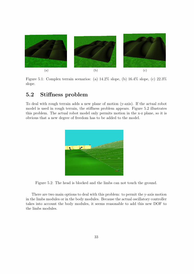
(a) (b) (c)

Figure 5.1: Complex terrain scenarios: (a) 14.2% slope, (b) 16.4% slope, (c) 22.3%slope.

5.2 Stiffness problem

To deal with rough terrain adds a new plane of motion (y-axis). If the actual robotmodel is used in rough terrain, the stiffness problem appears. Figure 5.2 illustratesthis problem. The actual robot model only permits motion in the x-z plane, so it isobvious that a new degree of freedom has to be added to the model.

Figure 5.2: The head is blocked and the limbs can not touch the ground.

There are two main options to deal with this problem: to permit the y-axis motionin the limbs modules or in the body modules. Because the actual oscillatory controllertakes into account the body modules, it seems reasonable to add this new DOF tothe limbs modules.

33

5.3 New limbs module

The new DOF of the limbs module has a rotation motion between [−1.3, 1.3] radians.This new servo can be modeled as a complete passive joint or as a elastic joint.In Webots there exist three basic parameters to model this behaviour: maxForce,springConstant and dampingConstant. It seems obvious that if a totally passivebehaviour is desired, then maxForce, springConstant and dampingConstant haveto be set to zero. In the other hand, the optimal values of springConstant anddampingConstant are not known a priori. Moreover, it is not known which behaviourwill be better in any of the scenarios designed or which motion, rigid or oscillatory,will be optimal. This questions will try to be answered in next sections.

Figure 5.3: New limbs module. The red line represents the new y-axis rotation DOF.

5.4 Webots issues

Until experimenting in rough terrain, collisions were calculated taking into accountthe body shape of the module and the foot shape. The bounding object shape ofthe body and limbs module was a box, but the foot was considered as a cylinder.Webots can not calculated collisions between a triangle mesh and a cylinder so itwas mandatory to change the limbs boundingObject node. Figure 5.4 illustrates thisissue.

After correcting the model to make it able to climb over rough terrain, anotherproblem was discovered. Every hill is modeled as a triangle mesh and if the trianglesdensity is not enough high, the centipede’s foots would be able to go through the

34

(a) (b)

Figure 5.4: Bounding box models: (a)cylinder and (b)box.

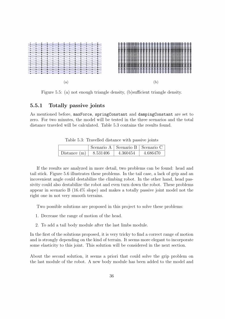
hill object. This was a serious problem because of the incorrectness of the simula-tion. Fortunately, the problem was solved re-modeling the hills with a high triangledensity. Table 5.2 contains the triangle mesh error and the conversion error used inArt of Illusion application. Figure 5.5 illustrates the difference triangle density in therendering of the hill. The density of triangles was also a critical parameter in thesimulation time, so it was a trade off between accuracy of collisions and time spendton 3D rendering. The values from table 5.2 represent a good rendering density and agood simulation time.

Table 5.2: Triangle mesh rendering errors

Scenario A Scenario B Scenario CTriangle mesh error 0.0025 0.005 0.005

Object rendering error 0.05 0.05 0.05

5.5 Rigid body controller in complex terrain

First of all, the totally passive joints will be tested in the three different scenarios.Then, a quick search over the spring and damper constants will be made and the bestresults found will be compared with the totally passive results.

35

(a) (b)

Figure 5.5: (a) not enough triangle density, (b)sufficient triangle density.

5.5.1 Totally passive joints

As mentioned before, maxForce, springConstant and dampingConstant are set tozero. For two minutes, the model will be tested in the three scenarios and the totaldistance traveled will be calculated. Table 5.3 contains the results found.

Table 5.3: Travelled distance with passive joints

Scenario A Scenario B Scenario CDistance (m) 8.531406 4.360454 4.686470

If the results are analyzed in more detail, two problems can be found: head andtail stick. Figure 5.6 illustrates these problems. In the tail case, a lack of grip and anincovenient angle could destabilize the climbing robot. In the other hand, head pas-sivity could also destabilize the robot and even turn down the robot. These problemsappear in scenario B (16.4% slope) and makes a totally passive joint model not theright one in not very smooth terrains.

Two possible solutions are proposed in this project to solve these problems:

1. Decrease the range of motion of the head.

2. To add a tail body module after the last limbs module.

In the first of the solutions proposed, it is very tricky to find a correct range of motionand is strongly depending on the kind of terrain. It seems more elegant to incorporatesome elasticity to this joint. This solution will be considered in the next section.

About the second solution, it seems a priori that could solve the grip problem onthe last module of the robot. A new body module has been added to the model and

36

(a) (b)

Figure 5.6: (a) Head stuck (b) Tail stuck.

the experiments have been run again. This tail module could be rigid or passive. Arigid joint in the last module could produce again a stiffness problem in some kind ofterrains, so a passive joint is proposed. Table 5.4 shows the obtained results.

Table 5.4: Travelled distance with passive joints and an extra tail module.

Scenario A Scenario B Scenario CDistance (m) 6.840540 3.412944 3.122146

These results have to be analyzed in context. Scenario A is obviously worse withthe extra tail module. In both scenarios the robot is able to climb. But in scenariosB and C without the extra tail module, the robot was unable to climb. In scenarioB with the extra tail module, the robot is able to climb, so it seems to solve theproblem. Again, in scenario C, the slope is as pronunciate as the robot is unable toclimb, with or without this new tail module. It is not absurd to confront the robotwith a 22.3% slope in a real world scenario so finally the solution of the extra tailmodule has to be discarded.

5.5.2 Spring and damped joints

In a model with a single spring and a single damper, the torque can be expressed asequation 5.1.

T = −ωθ − µθ̇ (5.1)

37

(a) (b)

Figure 5.7: (a) 16.4% slope. Red arrow points to the extra module. (b) Final positionof the extra module added model in a 22.3% slope scenario. The robot is not able toclimb.

Where ω is the spring constant and µ the damping constant.

Figure 5.8: Simple mass-spring-damper system. Reprinted from [13] with permission.

A priori, it is not known which values of ω and µ could be the best performingones. But there exist some restrictions in their values that can delimit the search:

• Variable ω ∈ (0, 20] (Nm).

• Variable µ ∈ (0, 0.1] (Nsm).

Values of this variables higher than the interval maximums could cause a explosionof the model in Webots and the incorrectness of the simulation or even the turning

38

down of the robot because of the up and down oscillations.

Figure 5.9: Model explosion in Webots simulation.

Table 5.5: Travelled distance (m) depending on ω and µ in scenario A.

ω/µ 0.0 0.01 0.03 0.05 0.1 0.20 – 8.6878 10.3678 12.3852 19.9515 Unstable10 Unstable 25.6199 24.8168 24.9136 Unstable Unstable20 Unstable 25.5145 24.9341 Unstable Unstable Unstable

A quick search over the possible values of the spring and damping constant (limbsfrequency equal to 1.0 Hz and phase difference between limbs of π

2, best results ob-

tained for the rigid body controller in Chapter 4) gives the results from table 5.5. Thelabel Unstable means that there was some problem in the simulation as high changeof motion direction due to the high oscillations introduced by the new DOF or evena turning down of the robot.

Some observations can be remarked analyzing the data:

• For bigger values of the spring and damping constants, the behaviour becomesunstable.

• When the spring constant is set to zero and for small values of the dampingconstant, the behaviour is quite similar to the totally passive joints.

• Higher values of the spring constant introduces oscillations that propagate fromthe head to the tail causing undesirable changes of the direction.

39

In conclusion, only elasticity is desirable in rough terrain, not in flat terrain. Asmall value of the spring constant could help to improve the total performance and ahigh value of the damping constant cushions undesirable oscillations along the bodyshape and could help to adapt to the terrain maintaining some stiffness. Taking thisassumptions into consideration, some recommended values for the spring and damp-ing constants are ω ∈ [1, 5] and µ ∈ [0.05, 0.1]. These values between the intervalsalmost perform in the same way in the three different scenarios and they remain opento depend on real physics characteristics of the material used to build the joint.

The stiffness problem has been solved thanks to the new spring-damped joint. Thequality of the locomotion behaviour using springs and dampers has been found usinglow values for the spring constant and high values (taking into account the allowedinterval) of the damping constant. Some quick simulations using that parametershave performed in a similar way, but this performance depends on the terrain: biggerslope, lower traveled distance. In next sections the values of ω and µ will be fixed to2 Nm and 0.1 Nsm respectively.

5.6 Oscillatory body controller in complex terrain

In Chapter 4 has been demonstrated that the oscillations along the body shape of therobot were able to improve the speed of locomotion. A very good solution was found,improving the performance over a 80% of the speed using the oscillatory controllerinstead of the rigid body one. In last section the spring-damped joints have beenincorporated to the model allowing the robot to climb over slopes till 22.3%, so itseems reasonable to incorporate this joints to the model using the oscillatory bodycontroller. The questions that have to be answered in this section are:

• An oscillatory body controller is able to climb over complex terrain?

• Is the best solution found in flat terrain one of the most performing ones incomplex terrain?

• An oscillatory body controller can improve again the performance obtained withthe rigid body controller, this time in complex terrain?

5.6.1 An oscillatory body controller is able to climb overcomplex terrain?

The answer is yes, it is able, but it seems to be totally depending on the amplitude ofthe travalling wave over the body length. The straight line seems to be the faster wayto climb over the obstacles that take part of the designed scenarios, so the value ofthe parameters of the oscillatory controller that can guarantee a locomotion proximalto the straight line will be the best ones.

40

5.6.2 Is the best solution found in flat terrain one of the mostperforming ones in complex terrain?

To answer this question, a new experiment has been designed. This experiment isexactly the same experiment as in section 4.3, but now testing in different complexterrain scenarios. Experiment parameters are presented below:

• Simulation time of 20 seconds.

• Phase angle difference between limbs fixed to π2.

• Limbs controller parameters rest with the same valour as in section 4.3.

• Frequency (angular speed ω) fixed to 1.0 Hz.

• Phase angle between limbs and body (ϕ) parameter searching interval from −πto π with a step of π

4.

• Phase angle between body modules (∆ϕ) parameter searching interval from −πto π with a step of π

4.

• Amplitude of the body servo (Ak) parameter searching interval from 0.1 to 1.0with a granularity of 0.05.

• Speed is integrated at each timestep as a continuous speed and is also savedmean speed, total distance traveled and angle between origin and final position.

In section 4.3 experiment, the mean speed was the interesting parameter. Incomplex terrain, to measure the quality of the solution the total distance traveled(end position minus start position) and the heading angle between initial and finalposition will be the studied variables. Before continuing, the obstacles area has tobeen defined. Obstacles area is the hills matrix NxM zone. In the experimentscenarios, a sufficient large obstacles are has been designed to ensure that in theexperiment simulation time (fixed to 20 seconds) the robot if is able to climb, it willbe inside this region.

To ensure that the solutions found are the most performing ones, two filters fordata have been designed:

• Not in the obstacle area. This rule filters the solutions that at the final of thesimulation are not inside of the obstacle area. Note that is impossible to reachthe opposite region of the obstacle area in less than 20 seconds (simulationexperiment time).

• Error angle. This rule filters the solutions that the angle between initial andfinal positions don’t respect the tolerable straightness error. Solutions betweenthe interval [π

2− π

3, π

2+ π

3] radians will be only accepted (ε = 16.6%).

41

Figure 5.10: The red line delimits the obstacles area.

In a first iteration of the experiment one new problem is found: due to N=3 inobstacles area, in oscillatory mode the robot is very probable thats falls down the hillor even turn, increasing the noise of the results found. To avoid this problem, N isfixed to 1, but preserving the same slope. Figure 5.11 shows the new scenarios.

Figures 5.12, 5.13 and 5.14 present the results of the experiment in scenarios A,Band C respectively and corrected with the filters mentioned before. Table 5.6 showsthe mean and the standard deviation of the traveled distance in every scenario.

Table 5.6: Travelled distance mean (µ), standard deviation (σ) and maximum value.

Scenario A Scenario B Scenario Cµ 3.4417 2.7773 3.2338σ 1.2224 1.2029 1.2357

max 7.0620 7.9857 7.6415

At first sight, a high standard deviation on every scenario is emphasized. Thisis due to the high variability of locomotion gaits tested on the experiment. Themaximum values can be also quite confusing if there are not put in context. Itseems reasonable to cover less distance with a higher slope. This issue is followed onscenarios B and C. The maximum of the traveled distance is the smaller in scenario

42

(a) (b) (c)

Figure 5.11: Complex terrain scenarios: (a) 14.2% slope, (b) 16.4% slope, (c) 22.3%slope.

A because of its construction: M = 4 and in scenarios B and C, M = 2. While inscenario A, in the established simulation time, the robot can cover two hills and climbtwo times, in scenarios B and C this possibility does not exist.

Another good appreciation is that the filters seems to affect in each scenario in thesame variables interval (regions set to zero). This is a proof of the future robustness ofthe best solutions found because they will perform almost in the same way in differentscenarios. For every scenario, the best solutions are analyzed below:

Scenario A . The best solution found is the same as in flat terrain (Ak = 1.0,∆ϕ = −π

2and ϕ = 0) and is consistent with the data found in Chapter 4, due

to the slight slope of this scenario.

Scenario B . In this scenario, the best solution found in flat terrain is one of themost performing ones, but not the best: traveled distance of 6.38 meters versus7.98 meters of the best. In this scenario the most performing solutions have incommon the property of a small lateral bending on the oscillation motion. Thisissue points that the rigid body could be the best solution in obstacles areas.

Scenario C . In this scenario, the best solution found in flat terrain is again themost performing one.

Whom could ask himself which is the critical difference between scenarios B andC to explain this difference. It seems to be a lot of parameters playing an importantrole in the best solution: characteristics of the terrain that can be profited by theundulations to climb in a better way, the chosen joints stiffness, etc. Next sectionwill try to explain this issues comparing the behaviour between the rigid body andthe oscillatory body controllers.

43

(a) (b) (c)

(d) (e) (f)

(g) (h)

Figure 5.12: Travelled distance in scenario A with oscillatory controller.

44

(a) (b) (c)

(d) (e) (f)

(g) (h)

Figure 5.13: Travelled distance in scenario B with oscillatory controller.

45

(a) (b) (c)

(d) (e) (f)

(g) (h)

Figure 5.14: Travelled distance in scenario C with oscillatory controller.

46

5.6.3 Complex terrain: is there any profit chosing an oscil-latory controller instead of a rigid one?

To answer this question, both controllers will be tested again on scenarios from Fig-ure 5.11. The parameters used in this test are detailed in Table 5.7.

Table 5.7: Complex terrain test parameters.

Rigid Body Oscillatory BodyFrequency (Hz) 1.0 1.0

Phase angle between limbs (rad) π2

π2

Amplitude Body (Ak) (rad) – 1.0Phase angle between body modules (∆ϕ) (rad) – −π

2

Phase angle between body and limbs (rad) – 0.0Spring Constant (Nm) 2.0 2.0

Damping Constant (Nsm) 0.1 0.1Simulation time (s) 20 20

The traveled distance covered by both controllers is detailed in Table 5.8.

Table 5.8: Covered distance (m)

Rigid Body Oscillatory BodyScenario A 3.94 6.37Scenario B 3.73 6.48Scenario C 3.43 5.97

It is interesting to observe that the improve is near 70%, but this improveness dif-fers slightly depending on the terrain and scenario. Before running the experiments,it was not obvious that an oscillatory controller perform better than the rigid one.One possible explanation could be that the oscillatory controller really increases thespeed of the robot and makes him climbing in a faster way than in a rigid controllercase.

The focus of this section was finding the relation between the rigid body and theoscillatory controller, but an important problem about the values found appeared.If the results are compared with the previous found, results from Table 5.8 in theoscillatory controller are slightly smaller. To find out the problem, the simulationswere rerun again, but without any difference. In any case, we have always been inter-ested in the qualitative solutions and the relationship between results and not in the

47

absolute values. The differences between hardware, triangle mesh density and ran-dom numbers generation inside the simulation could point to this difference betweenresults.

48

Chapter 6

Conclusions and Future work

Centipede robot locomotion is an approach to the extension of the salamander robot.During this project, different architectures have been presented and analyzed. Toreduce the research scope, one architecture was chosen because of its reliability andfeasibility: 16-legs centipede robot.Next step was finding good locomotion gaits in flat terrain. This work was inspiredin Manton theories [9] and Anderson group work [2]. The main goal was finding goodbehaviours and demonstrate if the oscillations along the body of the robot were beable to improve locomotion speed. Finally, a pure rigid body controller and the bestoscillatory gait were compared, with an increasing in the performance of the secondaround 80%. An increment of the speed was expected, but not as higher as has beenfound.After the work in flat terrain, the model and the best solution found in flat terrainwere confronted to complex terrain scenarios. Complex terrain implied a change inthe architecture of the robot to face irregularities of the terrain. New modules weredesigned taking into account actual constraints and two possible solutions were tested:totally passive joints and spring and damped joints. Finally, the second one repre-sented higher quality solutions and performance, so the spring and damped jointswere incorporated to the robot model.After that, different locomotion gaits were generated along the searching variablesspace of the oscillatory controller and, again, they were compared to a pure rigidbody controller. Oscillatory controller performance was over a 70% better than therigid body controller. This result was quite surprising because it not seems obviousa priori than an oscillatory controller could perform better in complex terrain thana rigid one. Moreover, best solution found in flat terrain was always one of the mostperforming locomotion gaits, a sign that confirm the robustness of this locomotiongait.

Due to the characteristics of Webots platform, all the experiments are easily re-producible again and this work will be a start point for real implementations of the

49

centipede robot model. Robot model physics have been simulated in detail, so it willbe reasonable to find the same behaviour in real hardware implementations. Futurework in the same scope of this project will imply research in:

• Developing of new central pattern generators (CPG) controllers based on thegood locomotion gaits found in this project to improve the robustness of thelocomotion.

• Including spring and damped joints in salamander robot to make it able towandering in complex terrain.

• Reproducing the experiments in real scenarios to validate simulations.

• Developing new legs modules and to check if the new models perform in thesame way.

50

Chapter 7

Annex: Media and Data CDOrganization

Several videos can be viewed and dowloaded from the project website at BIRG inhttp://birg.epfl.ch/page66520.html.

The data CD that encloses this project is organizated as:

• centipedescriptv2. Contains the source code and the CentipedeScript ex-ecutable.

• complex terrain models. Art of Illusion models files.

• controllers. Contains Webots controllers.

• doc. Bibliography used in this project.

• matlab. Matlab .m files scripts and figures obtained.

• media. Some graphical material.

• plugins. Physics plugin for Webots (standar centipede worlds do not use thisplugin).

• presentation. Mid-presentation of the project.

• report. This document, LATEXsources and figures.

• salamander. Salamander robot Webots project.

• videos. Generated videos and real scolopendra heros movies.

• worlds. Webots .wbt files.

51

Bibliography

[1] T. Allen, R. Quinn, R. Bachmann, and R. Ritzmann. Whegs ii: A mobile robotusing abstracted biological principles. 2004.

[2] B. D. Anderson, J. W. Schultz, and B. C. Jayne. Axial kinematics and muscleactivity during terrestrial locomotion of the centipede scolopendra heros. TheJournal of Experimental Biology, 198:1185–1195, 1995.

[3] K. Daltorio, S. Gorb, A. Peressadko, A. Horchler, R. Ritzmann, and R. Quinn.Wall-climbing mini-whegs. 2004.

[4] A. Ijspeert. A connectionist central pattern generator for the aquatic and ter-restrial gaits of a simulated salamander. Biological Cybernetics, 84(5):331–348,2001.

[5] A. Ijspeert, A. Crespi, and J. Cabelguen. Simulation and robotics studies ofsalamander locomotion. applying neurobiological principles to the control of lo-comotion in robots. Neuroinformatics, 3(3):176–196, 2005.

[6] A. Ijspeert, A. Crespi, D. Ryczko, and J. Cabelguen. From swimming to walkingwith a salamander robot driven by a spinal cord model. Science, 315:1416–1420,March 2007.

[7] D. E. Koditscheka, R. J. Fullb, and M. Buehler. Mechanical aspects of leggedlocomotion control. Arthropod Structure and Development, 33:251–272, 2004.

[8] S. Manton. The evolution of arthropodan locomotory mechanisms. iii. the lo-comotion of the chilopoda and pauropoda. J. Linn. Soc. (Zool.), 42:118166,1952.

[9] S. Manton. The evolution of arthropodan locomotory mechanisms. viii. func-tional requirements and body design in chilopoda, together with a comparativeaccount of their skeleto-muscular systems and an appendix on a comparisonbetween burrowing forces of annelids and chilopods and its bearing upon theevolution of the arthropodan haemocoel. J. Linn. Soc. (Zool.), 46:251484, 1965.

52

[10] S. Manton. The arthropoda: Habits, functional morphology and evolution. Ox-ford: Clarendon Press., 1977.

[11] R. Quinn, D. Kingsley, J. Offi, and R. Ritzmann. It’s got whegs. May 2002.

[12] R. E. Ritzmanna, R. D. Quinnb, and M. S. Fischer. Convergent evolution andlocomotion through complex terrain by insects, vertebrates and robots. ArthropodStructure and Development, 33:361–379, 2004.

[13] Wikipedia. Damping. 2007.

53