Calculation Techniques to Acquire Displacement

from Seismic Acceleration Records Y. Murono & H. Motoyama Earthquake and Structural Engineering, Structures Technology Division, Railway Technical Research Institute

SUMMARY: Computing displacement from measured acceleration is important for understanding the characteristics of an earthquake. However, to obtain such displacement with a good accuracy is difficult. It is partly because the low-frequency component dominating the behavior of the displacement is often affected by the sensor’s tilt and the measurement error. To avoid these, a high pass filter is usually applied; however, since this operation often distorts the acceleration record itself, we should apply it in a careful manner. In this paper, one methodology to obtain displacement from seismic acceleration records is hereby proposed. This method is composed with two methods; one to identify and remove the sensor's tilt motion, and the other to integrate a record by using only a real part of the Fourier transformation in consideration of causality. The adequacy of this technique is confirmed by applying the method to estimate the ground displacement of 2008 Iwate-Miyagi Inland Earthquake. Keywords: Residual displacement, Integration method in frequency domain, Tilt motion of sensors 1. INTRODUCTION In Japan, the high-density network of seismic stations has been developed to acquire vast of seismic data of earthquakes. Among the data, displacement of the ground is useful to estimate the earth motion. We often obtain displacement by twice integration of acceleration. However, while the low-frequency amplitude of acceleration is weak and easy to be damaged by noise, it dominates the behavior of the displacement, and through the process of the twice integration, the trend component appears in displacement wave which has no meaning in the term of physics. On the contrary, there are trend components, which we can describe physically. Near the fault, since the permanent displacement of the ground arises by the tectonic deformation, displacement waves do not return to zero. Moreover, although it is assumed that the seismometer has sensitivity only about the translation motion; the records from common pendulum type seismometer are affected by the rotation and the tilt motion. Simple integration of records including the rotation or tilt component generate displacement wave with trend component. Unlike the trend component caused by noise, these are not the physically meaningless. Incidentally, high-pass filter is commonly used for remove the trend component in displacement waveform. However, in recent digital strong-motion seismographs, the error factor is restricted, and applying a filter without careful consideration may distort the record obtained with sufficient accuracy. In this study, we propose the method focusing on (1) separating the rotation and translation motion and (2) removing the noise with careful consideration of not damaging the original waveform. 2. THE FACTOR OF TREND COMPONENT 2.1. Effect of the translation and rotation motion The most common sensor used in order to record earth motion is the pendulum type accelerometer. In most cases, it is assumable that the seismograph has sensitivity only about the translation motion. However, pendulum type seismographs produce the output also by (tilt or rotation) motion of the ground. Graizer has derived the equation of motion of the pendulum including rotation and tilt motion,

estimated the degree of incidence of each term from the sensitivity analysis by numerical analysis, and approximated equation of motion Equation (1).

211211111 2 ϕωω gxyyDy +−=++ &&&&&

122222222 2 ϕωω gxyyDy +−=++ &&&&&

33233333 2 xyyDy &&&&& −=++ ωω

(1)

where, iy : seismic records( i = 1,2: horizontal two directions, i = 3: vertical direction),

iω and iD :

the character frequency and the critical damping ratio of a converter, g : acceleration due to gravity,

ix&& : ground acceleration of i-th direction, and iϕ : rotation angle of ground motion around

ix . It can be said, the horizontal seismograph records the response to both the horizontal acceleration and tilt change, and the vertical seismograph records the response only to the vertical acceleration. Then, we briefly consider the effect of tilt change incorporated into the acceleration record. First, one acceleration record having only translation motion, as named a basic acceleration waveform, was prepared. The tilt component expressed by Equation (2) is added to this basic acceleration waveform.

( )( ) ( ) ( )[ ]

( ) ( )( )

<<>−+−−⋅−+−<

= 21

21

111

1

sin

expsin

0 0

ttt

ttttAB

ttttAttb

t

Tilt (2)

Where, A , B and b are constants, and 1t and

2t are the started and ended time of tilt component, respectively. Figure 1 shows a basic acceleration waveform and the incorporated tilt component. Although the tilt component is 0.045 degree which is equivalent to 0.5 gal and less than 1% of translation motion, the displacement waveform integrated simply from the waveform incorporated tilt change increases rapidly as shown in Figure 2. It can be checked that simple integration make a big trend component, even if the tilt component contained in the acceleration waveform is small. 2.2. Influence of FFT to a step function 2.2.1. Evaluation of a step function by the Fourier transform It is well known that the permanent displacement by the tectonic deformation, which is similar to a step function, is included in earthquake record in the hypocentral region of fault. Graves models acceleration and a displacement waveform as follows:

( ) ( )

−⋅⋅= 12

max 2sin

2tt

TT

Dta

ff

ππ

( ) ( ) ( )

−⋅−−= 1

max1

max 2sin

2tt

T

Dtt

T

Dtd

ff

ππ

(3)

In Equation (3), the displacement ( )td waveform as 1t = 0, fT =2, and Dmax=10 is considered (Figure

3). Figure 4 shows the waveform reproduced by IFFT of D(w), which is the theoretical Fourier spectrum of d(t). The dotted line shows original waveform and the solid line shows the waveform obtained by IFFT. Although step function is not a periodic function, the discrete Fourier transform (or FFT) treats the waveform as a periodic function. Therefore, this operation produces a big error and makes the waveform distorted. Thus, in treating a waveform including permanent displacement by the limited Fourier transform of FFT/IFFT, it turns out that an inescapable trend arises inevitably.

2.2.2. Influence of a high-pass filter A displacement waveform is calculated by integrating with the acceleration waveform given by Equation (3) using FFT. Figure 5 shows the acceleration waveform as

1t = 0, fT =2, and

maxD =10 in

Equation (3) and the displacement waveform integrated with the acceleration using FFT/IFFT. In this calculation, the high-pass filter often used is applied. The cutoff frequency

cf is 0.05 Hz. Permanent

displacement cannot be reproduced clearly but the meaningless long-period component has occurred. The real part ( )( )ωDℜ and the imaginary part ( )( )ωDℑ of the Fourier spectrum( )ωD , which are calculated theoretically from the displacement waveform, ( )td are as shown in Figure 6. The real part

( )( )ωDℜ has an upper limit in the low-frequency area. On the contrary, the amplitude of imaginary part ( )( )ωDℑ is greater in the lower-frequency area. When a high-pass filter removes the amplitude of low-frequency area, this operation has bigger influence to the imaginary part ( )( )ωDℑ than the real part ( )( )ωDℜ . Therefore, it can be considered that the less accurate reproducibility of permanent displacement as shown in Figure 5 is mainly caused by the cutoff of imaginary part. Hayashi et al. also pointed out this the same. 3. THE PROPOSAL OF THE CALCULATION METHOD OF DISPLACEMENT 3.1. The integration method

0 2 4 6 8 1002468

10

Dis

p (c

m)

Time (sec)

-10 0 1002468

10

Dis

p (c

m)

Time (sec) Figure 3 Step function Figure 4 Step function made by IFFT

-10

0

10

Dis

p(cm

)

0 2 4 6 8 10-20-10

01020

Acc

(ga

l)

Time(sec)0 2 4 6 8 10

Time(sec) Figure 5 Acceleration waveform( left) and Displacement waveform integrated by the usual FFT using

the high-pass filter( right)

0 10 20 30 400

1

2

Acc

(gal

)

Time (sec)

0 10 20 30 40-40-20

02040

Acc

(gal

)

Time (sec)

basic acceleration waveformtilt component

tilt component

0 10 20 30 40-1

0

1

2

3

Dis

p (c

m)

Time (sec)

basic waveformtilt component

Figure 2 Displacement waveform integrated from the acceleration waveform Figure 1 Basic acceleration waveform

and tilt component

In view of the above consideration, the following integration method is proposed by this research. Now, the target acceleration waveform is set to ( )ta . 3.1.1. Correction of baseline gap The arrival time of P wave is set to

pt , and then the baseline gap ε can be calculated from the data

before pt which is the area without any signal. The waveform ( )ta2

with correction of baseline gap

can be calculated by removing ε from the target acceleration waveform ( )ta . This baseline gap is interpreted as noise, which should be removed throughout the data. 3.1.2. Removal of a tilt component (refer to Section 3.2) The Fourier transform of ( )ta2

whose continuation time is dT is calculated. In order to clarify a step

function in acceleration waveform, many zero should be added after the data, and the number of total data is set to N= 1048576. By specifying the mixed tilt component from the obtained Fourier spectrum and removing this from acceleration waveform ( )ta2

, the waveform without the tilt component is calculated. 3.1.3. Integration using only Real part in frequency domain (refer to Section 3.3, 3.4) From the acceleration waveform ( )ta3

obtained above, the noise, which is defined by the cutoff

frequency, cf is removed (section 3.3). In addition, in order to make influence of a high-pass filter

into the minimum, displacement waveform d is calculated with integration in frequency domain only using the real part with consideration of causality (section 3.4). 3.2. Removal of the trapezoidal function resulting from tilt change As Section 2.1 described, a trend component occurs in a displacement waveform by the tilt motion. In order to argue simply, the tilt component expressed by Equation (2) is considered to be a step function (amplitudeA , and started time

0t ). Since the number of data for FFT FFTN should be involution of

two, zeros are generally added after earthquake record whose number of data is N .

Figure 7 Fourier spectrum of the acceleration waveform mixed tilt component

Figure 6 Real part and imaginary part of Fourier spectrum of step function

10-1 100 1010

1

2

Am

plit

ude

Frequency (Hz)

Real partImaginary part

10-4 10-3 10-2 10-1 100 10110-4

10-3

10-2

10-1

100

101

102

Am

plitu

de

Frequency (Hz)

Figure 8 Result of estimation of tilt component

0 10 20 30 400

1

2

Acc

(gal

)

Time (sec)

Mixed tilt component

Estimated tilt component

When the step function showing tilt change is mixing, to add zeros after the data is equivalent to add zeros after a step function, which makes the step function the trapezoidal function ( )ts . Fourier transform of trapezoidal function is as follows.

( )( )

0

02

1sin2

tid

e

tTA

S ω

ω

ωω −⋅

−⋅=

(4)

From Equation (4), the period of the Fourier spectrum of trapezoidal function is ( ) 20tTd − , Fourier

amplitude as 0=ω is ( )0tTA d − , and as ( )01 tTf d −= , Fourier amplitude is zero. By using these

information, the amplitude and the started time of the trapezoidal function (A and 0t respectively)

can be determined. Here, it verifies about the above-mentioned contents using the acceleration waveform (Figure 1) as used by examination of 2.1 and which is mixed tilt change artificially. Figure 7 shows the Fourier spectrum of the data which is made by adding zeros after Figure 1. Since

dT =59.99(sec),

( ) 0=ωSf =0.02345(Hz), and ( )0=ωS =21.11, we can obtain

st and A , as st =17.19(sec), A= 0.493. In

this case, tilt component is as shown in Figure 8. It turns out that the feature of the tilt component given artificially is estimated in general. 3.3. Removal of the noise in low-frequency area Generally, the low frequency content of observation record has the small signal to noise ratio, and the acceleration value of low frequency content acquired with the seismograph has a possibility of being polluted by the noise. In that case, when it integrates with acceleration waveform as it was and changes into a displacement waveform, a noise unrelated to the original earth motion is emphasized,

Figure 10 Estimated displacement for each level of the noise

Figure 9 Fourier spectrum of acceleration and noise

Figure 11 Decomposition of function with causality to odd function and even function

0 ,0 =< mym

my

omy

emy

10-2 10-1 100 10110-4

10-3

10-2

10-1

100

101

102A

mpl

itude

Frequency (Hz)

Level of noise:1 time

Basic waveformNoiseNoise mixed waveform

10-2 10-1 100 101 10-2 10-1 100 101

Level of noise:10 time Level of noise:100 time

Frequency (Hz) Frequency (Hz)

02468

10

Dis

(cm

)

Original wavefrom

0 20 40 60 8002468

10

Time (sec)0 20 40 60 80

Dis

(cm

)

Time (sec)

Level of noise: 10 times

Level of noise: 1 time Level of noise: 100 times

and it becomes totally different to the true displacement waveform. When the signal to noise ratio is large, simple integration works well, but when the signal to noise ratio is small, it is needed to apply a high-pass filter to remove the low-frequency content polluted by the noise. However, since there is a problem as described in section 2.2, cautions are required. Then, it will be examined what signal to noise ratio is needed for evaluating true displacement. Here, the basic acceleration waveform accompanied by permanent displacement is considered to an example. A noise is artificially added to this basic acceleration waveform. The level of the noise is made into 1 time, 10 times, and 100 times. The Fourier spectrum of each is as shown in Figure 9. Moreover, the displacement waveform by the proposed method is as shown in Figure 10. When a noise level is 100 times, the trend, which originated in the noise at the displacement waveform arises, and the amplitude of Fourier spectrum in the low-frequency area is crooked in V formation, which means that in this area the noise level is larger than the true signal. Therefore, when a spectrum is crooked, the high-pass filter whose cutoff frequency

cf is the crooked frequency should be applied.

3.4. Integration in consideration of causality Authors have drawn the relation between the real part and imaginary part of a Fourier transform of functions in time domain having causality. Here, details are passed over and the concept is shown briefly. The real time function my , which fills the causality, is defined by the sum of the even function

emy and the odd function o

my of Equation (5), as shown in Figure 11.

om

emm yyy += (5)

At this time, the even function emy and the odd function omy are related to the real part and imaginary

part of Fourier spectrum of the my by Fourier transform or Fourier inverse transform respectively. Furthermore, each function in time domain can be decomposed into a time restriction function and super function as shown in Fig. 11. Regarding real part, the operation of FFT/IFFT is possible, however, in the imaginary part a step function is contained and the Fourier transform has restriction for no periodic function; a linear trend will arise like a dotted line. That is, it turns out that the cause of the problem as described in 2.2.1 is using the imaginary part of the Fourier transform. Moreover, the imaginary part of a Fourier transform can be denoted by Equation (6) using a real part.

( ) ( )∑+−=

ℜ⋅=ℑ2

12

N

Nkklkl CC β

−= ∑−

= N

lm

N

km

N

N

mlk

ππβ 2sin

2cos

2 12

1

(6)

The Fourier spectrum of an acceleration waveform is calculated, and the Fourier spectrum of the displacement waveform ( )ωD is calculated by multiplying ( )21 ωi to the Fourier spectrum of an acceleration waveform. Then, the imaginary part ( )[ ]ωDℑ can be calculated from the real part

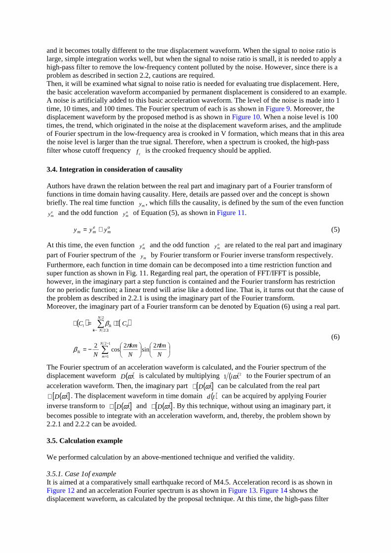
( )[ ]ωDℜ . The displacement waveform in time domain ( )td can be acquired by applying Fourier inverse transform to ( )[ ]ωDℜ and ( )[ ]ωDℑ . By this technique, without using an imaginary part, it becomes possible to integrate with an acceleration waveform, and, thereby, the problem shown by 2.2.1 and 2.2.2 can be avoided. 3.5. Calculation example We performed calculation by an above-mentioned technique and verified the validity. 3.5.1. Case 1of example It is aimed at a comparatively small earthquake record of M4.5. Acceleration record is as shown in Figure 12 and an acceleration Fourier spectrum is as shown in Figure 13. Figure 14 shows the displacement waveform, as calculated by the proposal technique. At this time, the high-pass filter

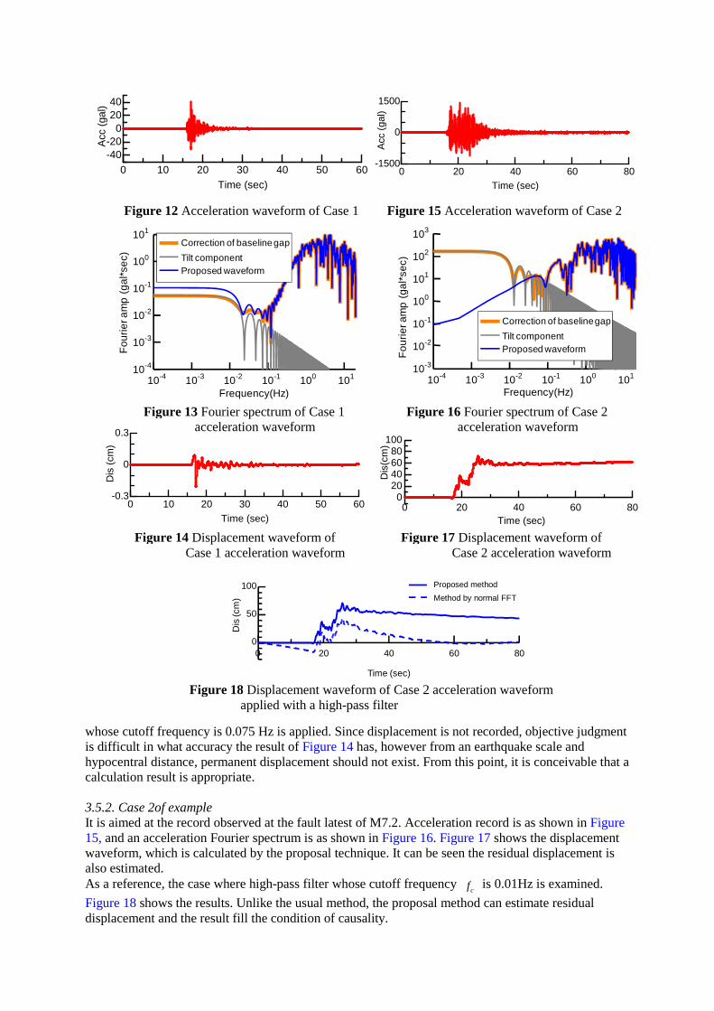
whose cutoff frequency is 0.075 Hz is applied. Since displacement is not recorded, objective judgment is difficult in what accuracy the result of Figure 14 has, however from an earthquake scale and hypocentral distance, permanent displacement should not exist. From this point, it is conceivable that a calculation result is appropriate. 3.5.2. Case 2of example It is aimed at the record observed at the fault latest of M7.2. Acceleration record is as shown in Figure 15, and an acceleration Fourier spectrum is as shown in Figure 16. Figure 17 shows the displacement waveform, which is calculated by the proposal technique. It can be seen the residual displacement is also estimated. As a reference, the case where high-pass filter whose cutoff frequency

cf is 0.01Hz is examined.

Figure 18 shows the results. Unlike the usual method, the proposal method can estimate residual displacement and the result fill the condition of causality.

Figure 13 Fourier spectrum of Case 1 acceleration waveform

Figure 12 Acceleration waveform of Case 1

0 10 20 30 40 50 60-40-20

02040

Acc

(ga

l)

Time (sec)

Figure 14 Displacement waveform of Case 1 acceleration waveform

0 10 20 30 40 50 60-0.3

0

0.3

Dis

(cm

)

Time (sec)

Figure 16 Fourier spectrum of Case 2 acceleration waveform

Figure 15 Acceleration waveform of Case 2

Figure 17 Displacement waveform of Case 2 acceleration waveform

0 20 40 60 80-1500

0

1500

Acc

(ga

l)

Time (sec)

0 20 40 60 800

20406080

100

Dis

(cm

)

Time (sec)

Figure 18 Displacement waveform of Case 2 acceleration waveform applied with a high-pass filter

10-4 10-3 10-2 10-1 100 10110-4

10-3

10-2

10-1

100

101

Fou

rier a

mp

(gal

*se

c)

Frequency(Hz)

Correction of baseline gap

Tilt componentProposed waveform

10-4 10-3 10-2 10-1 100 10110-3

10-2

10-1

100

101

102

103

Fou

rier a

mp

(ga

l*se

c)Frequency(Hz)

Correction of baseline gap

Tilt componentProposed waveform

0 20 40 60 800

50

100

Dis

(cm

)

Time (sec)

Proposed method

Method by normal FFT

4. APPLICATION TO IWATE-MIYAGI NAIRIKU EARTHQUAKE In this Chapter, the technique proposed in the preceding chapter is applied to the actually measured seismic waves. 2008 Iwate-Miyagi Inland Earthquake is selected. In the earthquake, the fault, which runs from north to south, shows the action of the reversed fault, and it has been one feature that earth motion seems opposite direction bordering on a fault. Applying the observation wave at this time, which residual displacement is calculated and compared with the earth motion. Six records from K-NET are tried and Figure 19 shows the results. Figure 19 also shows the measured displacement by GPS observation by Geographical Survey Institute. The argument concerning the accuracy is difficult; however, it is visible that the tendency can be estimated in general. The proposed integration technique is sufficiently practical, we conclude.

5cm

Higashi-NaruseMizusawa

Hiraizumi

Kurigoma

Naruko

Figure 19 Residual displacement of the calculation by proposal technique (left) and the measured

displacement by GPS (right) 5. CONCLUSION In integrating with acceleration record, it turned out that a trend occurs by the rotational component of earthquake record and by the noise in the low-frequency area where the signal to noise ratio is less. Then, we proposed the method to separate a rotation motion from the earthquake record, and extract only an translational motion, and the calculation technique to integrate acceleration waveform only using the real part of the Fourier spectrum for preventing a high-pass filter damaging the low-frequency component which the original records has as much as possible. We also verified applicability of proposed method by performing trial calculation to a real earthquake records. AKCNOWLEDGEMENT The K-NET records as used in this paper were observed by the National Research Institute for Earth Science and Disaster Prevention. REFERENCES Robert W. Graves: Processing issues for near source strong motion, Invited workshop on strong-motion record

processing, Convened by The Consortium of Organizations for Strong-Motion Observation Systems (COSMOS), Richmond, CA, 2004.

T. Sato and Y. Murono: Simulation of non-stationalry earthquake motion based on phase information, Journal of Japan Society of Civil Engineers, No.752, 2004.

Vladimir M. Graizer: Effects of tilt on strong motion data processing, Soil Dynamics and Earthquake Engineering, 25, pp.197-204, 2005.

Vladimir M. Graizer: Record processing considerations for the effects of tilting and transients, Proc. of COSMOS Strong Motion Workshop, Richmond, CA., 2004.

Vladimir M. Graizer: Tilts in strong ground motion, Bulletin of the Seismological Society of America, Vol.96, pp.2090-2102, 2006.

Y. Hayashi, H. Katsukura, T. Watanabe, S. Kataoka, H. Yokota and T. tanaka: Reliability of integrated displacements from accelerograms by digital accelerographs, Journal of Struct, No.419, 1991.