Acquiring Intangible Assets value calculation is even an ...€¦ · value of $54 million to...

Acquiring Intangible Assets

Intangible assets are important for corporations and their owners. The book value of intangible assets as a

percentage of total assets for all COMPUSTAT firms grew from 6% in 1990 to 13% in 2014. This book

value calculation is even an understatement, because assets on the balance sheet almost always excludes

intangible assets created within firms. Based on estimated values, Corrado and Hulton (2010) and Peters

and Taylor (2015) report that intangible assets constitute 34% to 45% of total assets. For the

unavailability of data on intangible assets, there is however little understanding on how they create value

to shareholders.

From June 2001, Statement of Financial Accounting Standards No. 141 requires that an acquirer allocates

purchase price to the fair value of identifiable intangible assets of the target (FASB, 2001), allowing us to

evaluate the importance of intangible assets in a merger and acquisition (M&A) context. Because

acquiring firms report the fair value based on their expected cash flow generated from intangibles, this

measure provides an unbiased expectation. We use data generated by this reporting requirement to answer

such important questions as: Why do firms acquire intangible assets? Do such acquisitions create value?

What is the exact channel of value creation?

Two commonly cited motivations of M&A activities focus on the creation and destruction of shareholder

wealth. We apply them to study the acquisition of intangibles. The neoclassical view argues that firms

purchase assets efficiently across industries they operate, so M&A activities benefit shareholders

(Maksimovic and Phillips, 2002). The other influential view in the literature is that entrenched managers

undertake M&A activities that reduce shareholder wealth (Jensen, 1986; Morck, Shleifer, and Vishny,

1990). Although there is a large literature supporting both views, almost all papers consider acquired

assets homogeneously. Said differently, the valuation effects of acquiring tangible assets are well known,

but the effects of acquiring intangible assets are still an unresolved question.

It also remains an unresolved question as to what creates value. Under the neoclassical view, shareholder

value is created either through wealth transfers from other stakeholders or through economies of scale,

synergistic gains, and better managerial skills. Kim and Singal (1993) analyze the airline mergers and find

that merged firms immediately gain from less competitive pricing, which is consistent with the increased

market power hypothesis. Focarelli and Panetta (2003) emphasize analysis on longer periods to test the

efficiency hypothesis, because realizing improvements in efficiency takes time. They find that efficiency

gains dominate over the market power effect in the long run. Analyzing product quality and price of

merged firms, Sheen (2014) also documents that operational efficiencies materialize in two to three years.

Considering a long-term horizon, Healy, Palepu, and Ruback (1992) similarly document post-merger

improvements in operational efficiency. On the entrenchment view, Harford, Humphery-Jenner, and

Powell (2012) find that managers choose low synergy targets and avoid all-equity payments when

acquiring private firms or public firms with blockholders.

This paper evaluates the above hypotheses in relation to intangible assets. After 2001, firms report

significant prices to purchase intangibles. For example, Procter & Gamble paid nearly 50% of the deal

value of $54 million to acquire Gillette’s brand in 2005. Using hand-collected data on 1,481 mergers and

acquisitions between 2002 and 2005, we also find that a typical acquirer in our sample pays 25% of the

deal value to purchase intangible assets, which includes brands, trademarks, service marks, patents, legal

contracts, etc.

Our analysis begins with investigating the determinants of acquiring intangibles. Modeling the likelihood

of intangible assets acquisition, we find lower levels of debt, operating performance, and capital

expenditures as important acquirer characteristics. However, when we model the amount of intangible

assets as a percentage of deal value, we find that acquirers of intangibles are smaller in size and incur less

capital expenditures, but spend more on R&D expenses. Overall, the finding that intangible asset

acquirers allocate significantly lower amount of resources on capital expenditures leading to acquisitions

resonates across models. Along with our later finding that these acquirers continue reducing capital

expenditures after the acquisition, this result suggests the tightening of acquirer industry.

We next explore market reactions of intangible asset acquisition. While the five day cumulative abnormal

return (CAR) of the whole sample is 0.85%, there is significant variability across acquisition of intangible

assets. Specifically, firms that do not acquire intangibles experience only 0.07% abnormal return. The

acquirer CAR then monotonically increases across terciles, ending with the highest CAR of 1.56% (p-

value = 0.00) for the third tercile of firms acquiring the highest amount of intangible assets. The

multivariate regression analysis that controls for a host of control variables also documents a similar

result. Specifically, we find that a 10% increase in the acquisition of intangible assets is associated with a

2.73% higher CAR, which is significant at the 1% level. Moreover, the effect is significantly more

pronounced if the target is a public firm, suggesting that acquirer shareholders benefit more from the

management of intangible assets of public targets. Overall, we document that acquiring intangible assets

monotonically increases shareholder wealth.

Our subsequent tests analyze the sources of value creation. To evaluate the effect of intangible asset

acquisition to subsequent performance, we categorize acquirers at the time of M&A announcements. We

create terciles of acquirers based on their purchase of intangibles and track their performance after

acquisitions. We also assign firms that do not acquire any intangible assets to a different portfolio and use

it as a cross-sectional benchmark. We then calculate different ratios based on acquirer three year average

performances before and after acquisition to measure the effect of intangible asset acquisitions. Beginning

with return on asset (ROA), we find that firms not acquiring intangibles experience increased

performance that is not statistically significant. However, post-merger firm ROA improves monotonically

with higher amount of intangible asset acquisition. We document the highest ROA increase of 8.8% for

the third tercile, which is significant at the 5% level.

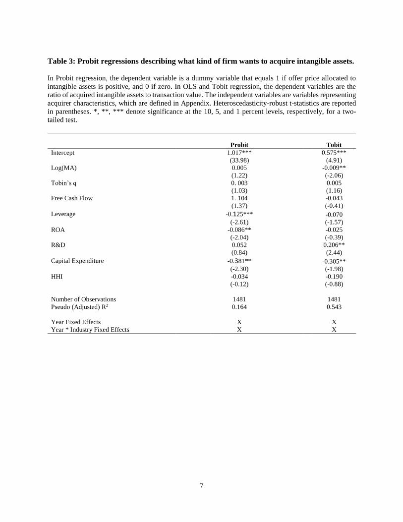
To further investigate the underlying mechanism of the increased ROA, we calculate its two components:

pre-tax operating margin and asset turnover. The pre-tax operating margin measures profits on a dollar of

sales and the asset turnover ratio indicates operational efficiency. We again do not find any significant

changes for acquirers that do not purchase intangible assets. However, we find significant improvements

in the pre-tax operating margin that increases with more acquisition of intangible assets. The asset

turnover ratio reduces for all acquisitions of intangible assets. These results do not support Healy, Palepu,

and Ruback (1992)’s finding on the efficiency gains after M&A activity. We also find that firms

acquiring the most intangible assets reduce R&D and capital expenditures drastically: R&D expenses

reduce from 9% before the year of acquisition to 4.2% after ten years, whereas capital expenditures drop

from 7% to 2.7%. During the same event time period, the average acquirer in the third tercile increases its

market share from 8.3% to 14.1% while the number of firms in the acquirer industry drops by 26%. These

results suggest that acquirers of intangible assets benefit from

Table 1: Sample Distribution by announcement year and intangible assets acquisition.

The table describes our sample of merges and acquisitions from 2002 to 2005 listed on SDC where U.S.

public acquirer who discloses offer price allocation gains control of a public, private, or subsidiary target

whose transaction value is at least $1 million and 1% of the acquirer’s market value.

Panel A:

Announcement

Year

Number of

deals

Acquirer

market

value

($mil)

Deal

value

($mil)

Acquired

Intangible

Assets

($mil)

Acquired

Intangible

Assets

/ Deal value

(%)

5-days CAR

(%)

2002 295 1,987 188 154 24 1.457

2003 336 2,477 248 63 27 0.842

2004 406 2,397 353 51 25 0.647

2005 444 3,793 446 195 26 0.642

Overall 1481 2,752 324 117 25 0.850

5

Table 2: Acquirer, target, and deal characteristics.

The sample consists of 1481 completed U.S. mergers and acquisitions listed on SDC from 2002 to 2005

made by acquirers who disclose offer price allocations.

Panel A: Whole Sample Mean St Dev Q1 Median Q3

Acquirer characteristics

Market value of equity ($mil) 2,752 8,782 178 507 1,455

Market value of assets ($mil) 4,478 15,285 223 707 2,082

Leverage 0.183 0.178 0.028 0.132 0.301

Tobin’s q 2.461 2.210 1.141 1.727 2.733

Free cash flow -0.004 0.157 -0.014 0.034 0.078

Stock price run-up 0.186 0.564 -0.146 0.068 0.325

Deal characteristics

Transaction value 324 1,010 17 50 166

Relative size 0.204 0.278 0.046 0.102 0.244

Competed deals (dummy) 0.009 0.093 0.000 0.000 0.000

Cash in payment (%) 0.626 0.411 0.210 0.810 1.000

Pure cash deals (%) 0.429 0.495 0.000 0.000 1.000

Pure equity deals (%) 0.092 0.289 0.000 0.000 0.000

Tender-offers (%) 0.020 0.141 0.000 0.000 0.000

Hostile 0 0 0 0 0

Public target (%) 0.228 0.420 0.000 0.000 0.000

Private target (%) 0.504 0.500 0.000 1.000 1.000

Subsidiary target (%) 0.268 0.443 0.000 0.000 1.000

High tech (dummy) 0.314 0.464 0.000 0.000 1.000

Diversifying (dummy) 0.207 0.405 0.000 0.000 0.000

Industry M&A 0.052 0.038 0.026 0.040 0.082

Panel B: Sample with intangible assets Mean St Dev Q1 Median Q3




Leverage 0.176*** 0.174 0.026 0.126 0.286

Tobin’s q 2.505*** 2.239 1.147 1.780 2.774

Free cash flow -0.004 0.159 -0.013 0.035 0.078




Relative size 0.196*** 0.265 0.046 0.099 0.241


Cash in payment (%) 0.627 0.410 0.210 0.810 1.000

Pure cash deals (%) 0.430 0.495 0.000 0.000 1.000


Tender-offers (%) 0.021 0.144 0.000 0.000 0.000

6

Hostile 0 0 0 0 0

Public target (%) 0.232 0.422 0.000 0.000 0.000

Private target (%) 0.511* 0.500 0.000 1.000 1.000

Subsidiary target (%) 0.257*** 0.437 0.000 0.000 1.000

High tech (dummy) 0.332*** 0.471 0.000 0.000 1.000


Industry M&A 0.052 0.038 0.026 0.042 0.085

Panel C: Sample without intangible assets Mean St Dev Q1 Median Q3




Leverage 0.268 0.208 0.076 0.262 0.424

Tobin’s q 1.923 1.748 1.127 1.359 1.950

Free cash flow 0.004 0.134 -0.016 0.030 0.076




Relative size 0.297 0.393 0.051 0.124 0.447


Cash in payment (%) 0.611 0.418 0.100 0.795 1.000

Pure cash deals (%) 0.420 0.496 0.000 0.000 1.000


Tender-offers (%) 0.009 0.094 0.000 0.000 0.000

Hostile 0 0 0 0 0

Public target (%) 0.179 0.385 0.000 0.000 0.000

Private target (%) 0.420 0.496 0.000 1.000 1.000

Subsidiary target (%) 0.402 0.492 0.000 0.000 1.000

High tech (dummy) 0.098 0.299 0.000 0.000 1.000


Industry M&A 0.050 0.040 0.023 0.040 0.075

7

Table 3: Probit regressions describing what kind of firm wants to acquire intangible assets.

In Probit regression, the dependent variable is a dummy variable that equals 1 if offer price allocated to

intangible assets is positive, and 0 if zero. In OLS and Tobit regression, the dependent variables are the

ratio of acquired intangible assets to transaction value. The independent variables are variables representing

acquirer characteristics, which are defined in Appendix. Heteroscedasticity-robust t-statistics are reported

in parentheses. *, **, *** denote significance at the 10, 5, and 1 percent levels, respectively, for a two-

tailed test.

Probit Tobit

Intercept 1.017*** 0.575***

(33.98) (4.91)

Log(MA) 0.005 -0.009**

(1.22) (-2.06)

Tobin’s q 0. 003 0.005

(1.03) (1.16)

Free Cash Flow 1. 104 -0.043

(1.37) (-0.41)

Leverage -0.125*** -0.070

(-2.61) (-1.57)

ROA -0.086** -0.025

(-2.04) (-0.39)

R&D 0.052 0.206**

(0.84) (2.44)

Capital Expenditure -0.381** -0.305**

(-2.30) (-1.98)

HHI -0.034 -0.190

(-0.12) (-0.88)

Number of Observations 1481 1481

Pseudo (Adjusted) R2 0.164 0.543

Year Fixed Effects X X

Year * Industry Fixed Effects X X

8

Table 4: Regression analysis of announcement abnormal returns.

The dependent variable is the bidder’s five day cumulative abnormal return measured using the market

model. The independent variables are variables representing acquired intangible assets, product market

completion, acquirer characteristics, and deal characteristics, which are defined in Appendix.

Heteroskedasticity-robust t-statistics are reported in parentheses. *, **, *** denote significance at the 10,

5, and 1 percent levels, respectively, for a two-tailed test.

Panel A: Acquirers 5-days CAR

CAR (%) p-value N

without intangible assets 0.07 0.88 112 with intangible assets 1.26 0.00 1369

Low 0.26 0.29 457 1.23 0.00 456

High 1.56 0.00 456

Panel B: Regression Results

Variables

Intercept -0.313 0.450

(-0.08) (0.11)

Intangible/transaction_value 2.732***

(2.76)

Intangible/transaction_value * Public 5.037**

(1.96)

Intangible/transaction_value * Non-public 2.318***

(2.80)

Competitive Industry 0.226 0.231

(0.54) (0.55)

Unique Industry -0.679 -0.701

(-1.23) (-1.27)

Log(MA) -0.342*** -0.330***

(-2.58) (-2.48)

Tobin’s q 0.163 0.156

(1.16) (1.11)

Free Cash Flow -1.250 -1.200

(-0.61) (-0.58)

Leverage 2.938** 2.757**

(2.21) (2.08)

Stock Price Runup -1.533*** -1.514***

(-3.31) (-3.25)

Industry M&A 37.978 30.951

(0.99) (0.80)

Relative Size 3.040*** 3.117***

(2.93) (3.02)

High Tech 0.813 0.885

(0.91) (0.98)

High Tech * Relative Size -8.954*** -9.070***

(-2.70) (-2.73)

Diversifying -0.155 -0.143

(-0.28) (-0.26)

Tender Offer 0.145 0.032

(0.12) (0.03)

Competed 2.677 2.479

(1.21) (1.15)

9

Public -2.846*** --3.406***

(-4.84) (-4.79)

All Cash 0.220 0.193

(0.50) (0.44)

All Equity -1.388 -1.374

(-1.62) (-1.60)

Number of Observations 1481 1481

Adjusted R2 0.114 0.116

Year Fixed Effects X X

10

Table 5: Operating performance and investment policy

ROA Pre-tax operating margin Asset turnover

%intangible

Pre-merge

Post-merge

Difference N Pre-

merge Post-

merge Difference N

Pre-merge

Post-merge

Difference N

without intangible

0.028 0.097 0.069 34 -0.014 0.113 0.127 34 0.911 0.919 0.008 34

Low 0.011 0.035 0.024 140 0.096 0.146 0.050 140 0.770 0.567 -0.203** 140

-0.023 0.045 0.068** 139 -0.124 0.047 0.171** 139 1.088 0.760 -0.328*** 139

High -0.056 0.032 0.088** 139 -0.483 -0.037 0.446** 139 1.259 0.970 -0.289*** 139

R&D rate Capital Expenditure rate Non-debt tax shield

Pre-merge

Post-merge

Difference N Pre-

merge Post-

merge Difference N

Pre-merge

Post-merge

Difference N

without intangible

0.039 0.025 -0.014 35 0.096 0.065 -0.031 35 0.042 0.045 0.003 35

Low 0.045 0.024 -0.021* 152 0.045 0.020 -0.025*** 152 0.020 0.024 0.004 152

0.101 0.060 -0.041*** 152 0.061 0.027 -0.034*** 152 0.039 0.043 0.004 152

High 0.124 0.085 -0.039** 152 0.064 0.034 -0.03*** 152 0.041 0.052 0.011** 152

11

Table 6: Information Asymmetry

whole without

intangible Low Median High

Number of estimate 7 10 7 7 7 (8) (7) (8) (8) (7)

Forecast dispersion 0.09 0.09 0.07 0.10 0.12 (0.275) (0.081) (0.098) (0.349) (0.365)

N 226 12 72 71 71

Equity only (%) 21.1 21.6 24.6 20.0 18.5 (40.8) (41.4) (43.1) (40.0) (38.9)

Cash only (%) 40.6 40.5 34.7 40.1 46.9 (49.1) (49.3) (47.7) (49.1) (50.0)

Cash/deal (%) 63.9 62.5 56.3 64.7 71.0 (43.9) (41.9) (41.7) (40.0) (49.0)

Equity/deal (%) 36.1 37.5 43.7 35.3 29.0 (43.9) (41.9) (41.7) (40.0) (49.0)

Completion days 64 67 86 61 45 (73) (75) (84) (63) (62)

N 1481 112 457 456 456

12

Figure 2.Long-term activities

0.060

0.080

0.100

0.120

0.140

0.160

0.180

-1 0 1 2 3 4 5 6 7 8 9 10

Market Share

0

1

2

3

60

80

100

120

140

160

180

-1 0 1 2 3 4 5 6 7 8 9 10

# firms

0

1

2

3

0.000

0.020

0.040

0.060

0.080

0.100

0.120

-1 0 1 2 3 4 5 6 7 8 9 10

R&D

0

1

2

3

0.000

0.010

0.020

0.030

0.040

0.050

0.060

0.070

0.080

-1 0 1 2 3 4 5 6 7 8 9 10

Capex

0

1

2

3

13

0.02

0.025

0.03

0.035

0.04

0.045

-1 0 1 2 3 4 5 6 7 8 9 10

NDTS

0

1

2

3

-0.100

-0.080

-0.060

-0.040

-0.020

0.000

0.020

0.040

0.060

0.080

0.100

-10 -8 -6 -4 -2 0 2 4 6 8 10

ROA

0

1

2

3

-0.600

-0.500

-0.400

-0.300

-0.200

-0.100

0.000

0.100

0.200

0.300

-10 -8 -6 -4 -2 0 2 4 6 8 10

Healy

0

1

2

3

0.000

0.200

0.400

0.600

0.800

1.000

1.200

1.400

1.600

1.800

-10 -8 -6 -4 -2 0 2 4 6 8 10

turnover

0

1

2

3

14

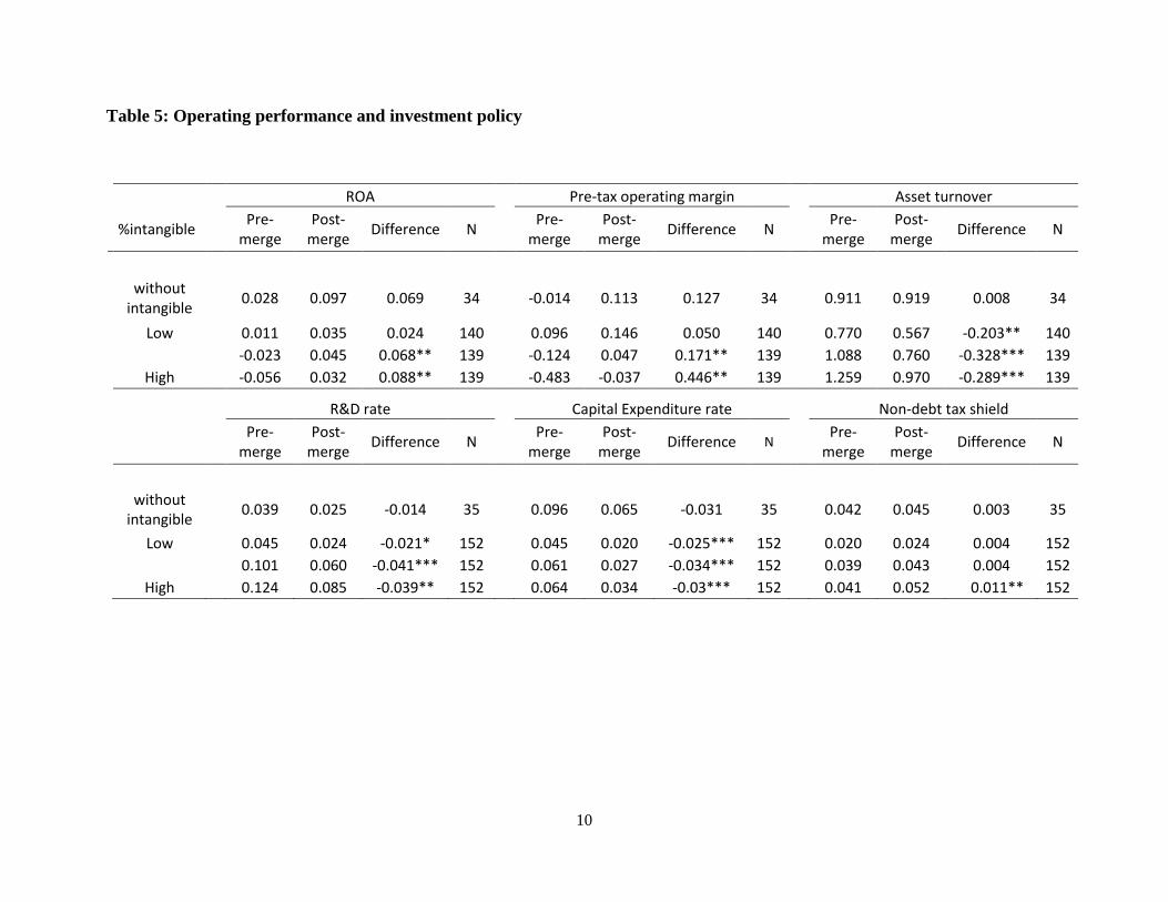
Appendix. Variable Definitions

CAR(-2,+2) Five-day cumulative abnormal return (in percentage points) calculated using the market model. The market model parameters

are estimated over the period (−210, −11) with the CRSP equally-weighted return as the market index.

Log(MA) Log(bookvalueoftotalassets + Fiscal-year-end market value of equity –book value of equity).

Tobin’s q (bookvalueoftotalassets + Fiscal-year-end market value of equity –book value of equity)/ book value of total assets.

Leverage (Long-termdebt + debt incurrentliabilities)/ book value of total assets.

Free cash flow (Operating income before depreciation– interest expenses– income taxes – capital expenditures)/ book value of total assets.

Stock price runup Bidder’s buy-and-hold abnormal return (BHAR) during the period (−210, −11). The market index is the CRSP value-weighted

return.

Pre-tax profit margin (EBIT + depreciation)/ sales.

ROA sales/market value of assets at the beginning of year (bookvalueoftotalassets + Fiscal-year-end market value of equity –book

value of equity).

R&D Research expenditures/ book value of assets at the beginning of year.

Capital expenditure Capital expenditures/ book value of assets at the beginning of year.

HHI

Public Dummy variable: 1 for public targets, 0 otherwise.

Private Dummy variable: 1 for private and subsidiary targets, 0 otherwise.

All cash Dummy variable: 1 for purely cash-financed deals, 0 otherwise.

All equity Dummy variable: 1 for purely equity-financed deals, 0 otherwise.

Diversifying acquisition Dummy variable: 1 if bidder and target do not share a Fama–French 12 industry, 0 otherwise.

Relative size Transaction value (from SDC)/acquirer market value of equity (Number of shares outstanding * the stock price at the 11th

trading day prior to announcement date).

High tech Dummy variable: 1 if bidder and target are both from high tech industries defined by Loughran and Ritter (2004), 0 otherwise.

Industry M&A The value of all corporate control transactions from SDC for each prior year and Fama–French 12 industry divided by the total

book value of assets of all Compustat firms in the same Fama–French 12 industry and year.

Tender offer Dummy variable: 1 for tender offer, 0 otherwise.

competed Dummy variable: 1 if there are multiple acquirers according to SDC, 0 otherwise.

Competitive industry

Dummy variable: 1 if the bidder’s industry is in the bottom quartile of allFama-French 48 industries' Herfindal-Hirschman

Index in the year prior to announcement, 0 otherwise. (calculated as the sum of squared market shares of all Compustat firms in

each industry ).

Unique industry Dummy variable: 1 if the bidder’s industry is in the top quartile of allFama–French 48 industries annually sorted by industry-

median product uniqueness, 0 otherwise. (calculated as selling expense scaled by sales).

Acquiring Intangible Assets value calculation is even an ...€¦ · value of $54 million to...

Documents

Transcript of Acquiring Intangible Assets value calculation is even an ...€¦ · value of $54 million to...