Building Cross-Sectional Systematic Strategies by Learning ...

*All articles are now categorized by topics and subtopics. View at PM-Research.com.

Building Cross-Sectional Systematic Strategies by Learning to RankDaniel Poh, Bryan Lim, Stefan Zohren, and Stephen Roberts

KEY FINDINGS

n Contemporary approaches (e.g., simple heuristics) used to score and rank assets in portfolio construction are sub optimal as they do not learn the broader pairwise and listwise relationships across instruments.

n Learning to rank algorithms can be used to address this shortcoming, learning the broader links across assets, which consequently allow them to be ranked more accurately.

n Using Cross-sectional Momentum as a demonstrative use-case, we show that more precise rankings produce long/short portfolios that significantly outperform traditional approaches across various financial and ranking-based measures.

ABSTRACT

The success of a cross-sectional systematic strategy depends critically on accurately ranking assets before portfolio construction. Contemporary techniques perform this ranking step either with simple heuristics or by sorting outputs from standard regression or classification models, which have been demonstrated to be suboptimal for ranking in other domains (e.g., information retrieval). To address this deficiency, the authors propose a framework to enhance cross-sectional portfolios by incorporating learning-to-rank algorithms, which lead to improvements in ranking accuracy by learning pairwise and listwise structures across instruments. Using cross-sectional momentum as a demonstrative case study, the authors show that the use of modern machine learning ranking algorithms can substantially improve the trading performance of cross-sectional strategies—providing approximately threefold boosting of Sharpe ratios compared with traditional approaches.

TOPICS

Big data/machine learning, portfolio construction, performance measurement*

Cross-sectional strategies are a popular style of systematic trading, with numer-ous flavors documented in the academic literature across different trading insights and asset classes (Baz et al. 2015). In contrast to time-series

approaches (Moskowitz, Ooi, and Pedersen 2012), which consider each asset inde-pendently, cross-sectional strategies capture risk premiums by trading assets against each other—buying assets with the highest expected returns and selling those with the lowest. The classical cross-sectional momentum (CSM) strategy of Jegadeesh and Titman (1993), for instance, selects stocks by ranking their respective returns over

Daniel Pohis a DPhil student with the Machine Learning Research Group and the Oxford-Man Institute of Quantitative Finance at the University of Oxford in Oxford, UK. [email protected]

Bryan Limis an associate member with the Machine Learning Research Group and the Oxford-Man Institute of Quantitative Finance at the University of Oxford in Oxford, [email protected]

Stefan Zohrenis an associate professor (research) with the Machine Learning Research Group and the Oxford-Man Institute of Quantitative Finance at the University of Oxford in Oxford, [email protected]

Stephen Robertsis the RAEng/Man Professor of Machine Learning at the University of Oxford and the director of the Oxford-Man Institute of Quantitative Finance at the University of Oxford in Oxford, [email protected]

It is illegal to make unauthorized copies, forward to an unauthorized user, post electronically, or store on shared cloud or hard drive without Publisher permission., by guest on February 14, 2022. Copyright 2021 With Intelligence Ltd. https://jfds.pm-research.com/content/3/2Downloaded from

http://www.PM-Research.com

https://www.iijournals.com/topic/big-datamachine-learning

https://www.iijournals.com/topic/portfolio-construction

https://www.iijournals.com/topic/performance-measurement-0

mailto:[email protected]




The Journal of Financial Data Science | 71Spring 2021

the past year and betting that the order of returns will persist into the future—buying assets in the top decile and selling the bottom decile. By trading winners against losers, cross-sectional strategies have been shown to be more insulated against common market moves and to perform even when assets have non-negligible cor-relations (e.g., equity markets) (Baz et al. 2015; Jusselin et al. 2017; Roncalli 2017).

With the rise of machine learning in recent years, many cross-sectional system-atic strategies that incorporate advanced prediction models have been proposed (Kim 2019; Gu et al. 2018, 2019), often demonstrating significant improvements over traditional baselines. In general, these machine learning models are trained in a supervised fashion and aim to minimize the mean squared error (MSE) of forecast returns over the holding period. Although the regression models under this frame-work accurately provide a mean estimate of future asset returns, they do not explic-itly consider the expected ordering of returns, which is at the core of the design of cross-sectional strategies. This could have a negative impact on strategy performance and consequently lead to suboptimal investment decisions.

The limits of standard regression methods for ranking have been extensively stud-ied in information retrieval applications, with a number of metrics and methodologies proposed (Pasumarthi et al. 2019). Collectively referred to as learning to rank (LTR) (Li 2011), today’s variants make use of modern learning techniques, such as deep neural networks and tree-based methods (Wang and Klabjan 2017; Li et al. 2019; Wu et al. 2010)—leading to dramatic improvements in accuracy over simpler baselines. Although LTR algorithms have also been used to a small degree in finance, the majority of papers focus on their use in simple stock recommendations (Wang et al. 2019) and lack a framework for the development and evaluation of general cross-sectional strategies.

In this article, we show how LTR models can be used to enhance traditional cross-sectional systematic strategies, adopting CSM as a demonstrative use case. We first start by casting stock selection as a general ranking problem, which allows for the flexibility of switching between different LTR algorithms and incorporating state-of-the-art models developed in other domains. Next, we concretely evaluate LTR models against a mixture of standard supervised learning methods and heuristic benchmarks. Through tests on US equities, we demonstrate that the pairwise and listwise models substantively improve the ranking accuracy of stocks, leading to over-all improvements in strategy performance with the adoption of LTR methods. Finally, although our ranking algorithms make use of momentum predictors, their modular nature allows these inputs to be adapted to incorporate other feature sets, thus providing a novel and generalizable framework for general cross-sectional strategies.

RELATED WORKS

Cross-Sectional Momentum Strategies

Momentum strategies can be categorized as (univariate) either time series or (mul-tivariate) cross-sectional. In time series momentum, an asset’s trading rule depends only on its own historical returns. It was first proposed by Moskowitz, Ooi, and Pedersen (2012), who documented the profitability of the strategy in trading nearly 60 different liquid instruments individually over 25 years. This has prompted numerous subsequent works (Baz et al. 2015; Rohrbach and Suremann 2017; Lim, Zohren, and Roberts 2019) that explore various trading rules alongside different trend estimation and position sizing techniques that are aimed at refining the overall strategy.

CSM employs a similar idea but focuses on comparing the relative performance of assets. It is characterized by first sorting the instruments by performance (typically taken to be returns) and then buying some fraction of top performers (winners) while selling a similar-sized fraction of underperformers (losers). Since the earlier work by Jegadeesh and Titman (1993), who considered this strategy for US equity markets, the


72 | Building Cross-Sectional Systematic Strategies by Learning to Rank Spring 2021

literature has been replete with a spectrum of works, ranging from those that report the existence of the momentum phenomenon in other markets and asset classes (LeBaron 1996; Rouwenhorst 1998; Griffin, Ji, and Martin 2003; Erb and Harvey 2006; Chui, Titman, and Wei 2010; de Groot, Pang, and Swinkels 2012) to others that propose new ways to improve various aspects of the strategy. For instance, Kim (2019) performed ranking with the forward-looking Sharpe ratio instead of historical returns. Pirrong (2005) constructed rankings based on returns standardized by their respective volatilities, arguing that this allows for a fairer comparison of instrument performance; Baz et al. (2015) employed a similar but more sophisticated approach by using volatility-normalized moving-average convergence divergence (MACD) indicators as inputs. A common thread across recent works is their use of a regress-then-rank approach (Wang and Rasheed 2018)—minimizing return predictions against targets before ranking the outputs and finally constructing a zero-investment portfolio by trading the tails of the sorted results. Notably, the loss commonly employed is the MSE, which is a pointwise function; some examples of works training with the MSE include papers by Kim (2019) and Gu et al. (2019).

Surveying works related to CSM, we believe that this is the first article to consider the use of ranking algorithms to enhance CSM strategies. Instead of ranking based on heuristics or on outputs produced by models trained on pointwise losses, we propose using LTR algorithms, demonstrating that learning the pairwise and listwise structure across securities produces better ranking and consequently better out-of-sample strategy performance.

LTR in Finance

LTR is a key area of research in information retrieval that focuses on using machine learning techniques to train models to perform ranking tasks (Li 2011; Liu 2011). The information explosion along with modern computing advances on both the hardware (cloud-based GPUs and TPUs; see Google Cloud Cloud TPU documen-tation) and software (open-source deep learning frameworks such as TensorFlow [Abadi et al. 2015] and PyTorch [Paszke et al. 2019]) fronts have induced a shift in how machine learning algorithms are designed, going from models that required handcrafting and explicit design choices toward those that employ neural networks to learn in a data-driven manner. This has prompted a parallel trend in the space of ranking models, with researchers migrating from using probabilistic varieties such as the BM25 and Language Model for Information Retrieval that required no training (Li 2011) to sophisticated architectures that are built on the aforementioned devel-opments (Pasumarthi et al. 2019).

Today, LTR algorithms play a key role in a myriad of commercial applications such as search engines (Liu 2011), e-commerce (Santu, Sondhi, and Zhai 2017), and entertainment (Pereira et al. 2019). These algorithms have been explored to a more limited degree in finance, with specific applications in equity sentiment anal-ysis and ranking considered by Song, Liu, and Yang (2017) and Wang and Rasheed (2018). Song, Liu, and Yang (2017) applied RankNet and ListNet to 10 years of market and news sentiment data, demonstrating higher risk-adjusted profitability over the S&P 500 Index return, the HFRI Equity Market Neutral Index (HFRI EMN), and pure sentiment-based techniques. On the other hand, Wang and Rasheed (2018) documented the superiority of LambdaMART over standard neural networks in predicting intraday returns on the Shenzhen equity exchange, adopting order book–based features.

Despite the initial promising results, we note that these applications do not con-sider comparisons to traditional styles of systematic trading—with comparisons only performed against market returns by Song, Liu, and Yang (2017) and neural network models by Wang and Rasheed (2018)—making it difficult to evaluate the true value



added by LTR methods. The ranking methodologies are also customized to specific sentiment trading applications, making generalization to other types of cross-sectional trading strategies challenging. We address these limitations explicitly in our article, proposing a general framework for incorporating LTR models in cross-sectional strat-egies and evaluating their performance.

PROBLEM DEFINITION

Given a securities portfolio that is rebalanced monthly, the returns for a CSM strategy at τm can be expressed as follows:

rn

X rCSM i

i

ntgti

i

m m

m

m

m

m

m m

1,,

( )

1( ) ,

( )

1 1∑=σστ τ

ττ

= ττ τ+

τ

+ (1)

where τm, τm+1 ∈ T ⊂ 1, …, t - 1, t, t + 1, …, T and T denotes the set of indexes coinciding with the last trading day of every month; τ τ +

rCSM

m m, 1 is the realized portfolio

returns from month τm to τm+1; τnm refers to the number of stocks in the portfolio; and

∈ −τX i

m 1,0,1( ) characterizes the CSM signal or trading rule for security i. We rebal-

ance monthly to avoid excessive transaction costs that come with trading at higher frequencies (e.g., daily). We also fix the annualized target volatility stgt at 15% and scale asset returns with στ

i

m

( ), which is an estimator for ex ante monthly volatility. In this article, we use a rolling exponentially weighted standard deviation with a 63-day span on daily returns for στ

i

m

( ), but we note that more sophisticated methods (e.g., GARCH [Bollerslev 1986]) can be used.

Strategy Framework

The general framework for the CSM strategy comprises the following four com-ponents.

Score calculation. Presented with an input vector τui

m

( ) for asset i at τm, the strat-egy’s prediction model f computes its corresponding score τY i

m

( ):

uY fi i

m m( ).( ) ( )=τ τ (2)

For a cross-sectional universe of size τNm at τm, the list of scores of assets con-

sidered for trading is represented by the vector =τ τ ττY Y Y N

m m m

m , ..., (1) ( ) .Score ranking. The second component is computed as follows:

Z Yi i

m m( ) ,( ) ( )=τ τR (3)

with ∈τ τZ Ni

m m1, ..., ( ) being the position index for asset i after applying the operator

R(·) to sort scores in ascending order.Security selection. Selection is usually a thresholding step in which some frac-

tion of assets is retained to form the respective long–short portfolios. Equation 4 assumes that we are using the typical decile-sized portfolios for the strategy (i.e., top and bottom 10%).

=

− ≤ ×

> ×

τ

τ τ

τ τX

Z N

Z Ni

i

i

m

m m

m m

1 0.1

1 0.9

0 Otherwise

( )

( )

( ) (4)



Portfolio construction. Finally, simple portfolios can then be constructed by vola-tility scaling the selected instruments based on Equation 1.

In the following section, we provide an overview of score calculation techniques for both current strategy approaches and LTR models.

SCORE CALCULATION METHODOLOGIES

Most CSM strategies adhere to this framework and are generally similar over the last three steps (i.e., how they go about ranking scores, selecting assets, and constructing the portfolio). However, they are particularly diverse in their choice of the prediction model f used to calculate scores, ranging from simple heuristics (Jegadeesh and Titman 1993) to sophisticated architectures on an expansive list of macroeconomic inputs (Gu et al. 2018). Although numerous techniques to compute scores exist, they can be grouped into three categories: classical momentum and regress-then-rank (both of which are current approaches) and LTR, which is our pro-posed method.

Classical Cross-Sectional Momentum

Classical variants of the CSM tend to lean toward the use of comparatively simple procedures for the score calculation.

Jegadeesh and Titman (1993). The authors who first documented the CSM strategy proposed scoring an asset with its raw cumulative returns, computed over the past 3 to 12 months:

Y ri i

m m m: ,( )

252,( )=τ τ − τScore Calculation (5)

where τ − τr i

m m252,( ) is the raw returns over the previous 252 days (12 months) from τm

for asset i.Baz et al. (2015). A sophisticated alternative uses volatility-normalized MACD

indicators as an intermediate signal, forming the final signal by combining indicators computed over different time scales. The indicator is given as

= ξτ τ τ − τY zi i i

m m m m/std( )( ) ( )

252:( ) (6)

ξ = ττ τ − τi S L pim

i

m m mMACD( , , , )/std( )( )

63:( ) (7)

i S L m i S m i LmMACD( , , , ) ( , ) ( , ),τ = − (8)

where τ τp i

m mstd( )–63:

( ) represents the 63-day rolling standard deviation of security i, m(i, S) is an exponentially weighted moving average of prices for asset i, and S translates to a half-life decay factor HL = log(0.5) ⁄ log(1 - 1 ⁄S). The final composite signal com-bines different volatility-scaled MACDs over different time scales involving a response function f(·) and a set of short and long time scales Sk ∈ 8, 16, 32 and Lk ∈ 24, 48, 96 as set out by Baz et al. (2015):

∑= φτ=

τScore Calculation Y Y S Li

k

ik km m

( ): ( , ) .( )

1

3( ) (9)



Regress-Then-Rank Method

Newer works employing a regress-then-rank approach typically compute the score via a standard regression (refer to the “Cross-Sectional Momentum Strategies in the Related Works” section):

uY fi i

m m: ( ; ),( ) ( ) θθ=τ τScore Calculation (10)

where f characterizes a machine learning prediction model parameterized by q pre-sented with some input vector τu

i

m

( ) . Using the volatility normalized returns as the target, the model is trained by minimizing the loss, which is typically the MSE:

MY

r

Y r Y r

ii

i

N N N

m

m m

m

m

m

m m

m

m

m

( )1

( , / ), ..., ( , / ) ,

( ) ,( )

( )

2

(1),

(1) (1) ( ),

( ) ( )

1

1 1 2 1 1

1

1

1

1

1

∑θθ

= −σ

Ω = σ σ

ττ τ

τΩ

τ τ τ τ τ τ τ τ

+

−

τ −

−

τ −

−

τ −

L

(11)

where W represents the set of all M possible forecasted and target tuples over the set of instruments and relevant time steps.

LTR Algorithms

LTR methods can be categorized as being pointwise, pairwise, or listwise. The pointwise (pairwise) approach casts the ranking problem as a classification, regres-sion, or ordinal classification of individual (pairs of) samples, whereas the listwise approach learns the appropriate ranking model by using ranking lists as inputs. In terms of ranking performance, the pointwise method has been observed to be inferior relative to the last two techniques (Li 2011). Additionally, the loss function is not just the key difference across these models (Li 2011)—incorporating the pairwise and listwise information across assets makes LTR models collectively distinct from both the classical styles and regress-then-rank methods outlined previously.

We provide a high-level overview of four LTR algorithms that we use in conjunction with the momentum strategy, highlighting the loss function but omitting technical details to keep our exposition brief. For details on adapting the LTR framework for the momentum strategy, please refer to the section titled “Learning to Rank for Cross-Sectional Momentum” in the Appendix.

Burges et al. (2005) (RankNet). Although techniques that apply neural networks to the ranking problem already exist, RankNet was the first to train a network based on pairs of samples. Similar to contemporary methods, RankNet uses a neural net-work. Instead of minimizing the MSE, however, RankNet focuses on minimizing the cross-entropy error from classifying sample pairs, optimizing the network based on the probability that one element has a higher rank than the other. Because training is conducted on individual pairs using stochastic gradient descent, RankNet has a complexity that scales quadratically with the number of securities at rebalance time.

Burges (2010) (LambdaMART). LambdaMART is a state-of-the-art (Nguyen, Wang, and Kalousis 2016; Bruch 2020) pairwise method that combines LambdaRank (Burges, Ragno, and Le 2006) with multiple additive regression trees (MART). Inter-estingly, training in LambdaMART via LambdaRank does not involve directly optimizing a loss function but rather making use of heuristic approximations of the gradients (referred to as λ-gradients), exploiting the fact that only the gradients and not actual loss values are required to train neural networks. This allows the models to circumvent dealing with the often flat, discontinuous, and nondifferentiable losses such as the



normalized discounted cumulative gain (NDCG; Järvelin and Kekäläinen 2000), which is simultaneously a popular position-sensitive information retrieval metric and one that LambdaRank has been shown to locally optimize (Yue and Burges 2007; Donmez, Svore, and Burges 2009). Given the formulation of λ-gradients, the loss involves the product of a pairwise cross-entropy loss and the gain on some information retrieval metric (typically taken to be NDCG) (Wu et al. 2010). MART, on the other hand, is a tree boosting method known for its flexibility. It also offers a simple way to trade off speed and accuracy via truncation, which is important for time-critical applications such as search engines (Wu et al. 2010). LambdaMART, which is the result of mar-rying these methods, thus combines LambdaRank’s observed empirical optimality (with respect to NDCG) (Donmez, Svore, and Burges 2009) with the flexibility and robustness of MART.

Cao et al. (2007) (ListNet). ListNet was developed to address the practical issues inherent to pairwise techniques, such as their prohibitive computational costs and their mismatched objective of minimizing errors related to pairs classification instead of the overall ranking itself. ListNet resolves these problems by making use of a list-wise loss, adopting a probabilistic approach based on permutations. By first computing “top one” probability distributions over a list of scores and ground truth labels and then normalizing each with a softmax operator, the loss is defined to be the cross entropy between both distributions. By using the entire cross section of securities as inputs, ListNet has a complexity of ( )τO N

m—making it more efficient than RankNet,

which has a quadratic complexity of τO Nm

( )2 because training is conducted on pairs.Xia et al. (2008) (ListMLE). Seeking to analyze and provide more theoretical support

linking the choice of a ranking model’s listwise loss function to its corresponding performance, Xia et al. (2008) proposed the use of the likelihood loss owing to its nice properties of consistency, soundness, and linear complexity. Additionally, the like-lihood loss is continuous, differentiable, and convex (Boyd and Vandenberghe 2004). This culminated in the development of ListMLE, a probabilistic ranking approach that casts the ranking problem as minimizing the likelihood loss, or equivalently as maximizing the likelihood function of a probability model. ListMLE has been shown to outperform other listwise methods on benchmark datasets (Xia et al. 2008) and shares the same linear complexity as ListNet. Given our results, which we further discuss later in the article, we note that the benefit of the linear complexity possessed by both ListMLE and ListNet might be relevant for larger datasets.

Training Details

RankNet, ListNet, and ListMLE were trained with the Adam optimizer based on each model’s respective ranking loss function. Backpropagation was conducted for a maximum of 100 epochs in which, for a given training set, we partition 90% of the data for training and leave the remaining 10% for validation. As a matter of practicality, we set our target to be the returns 21 days ahead instead of the next month for training and validation. For LTR models using neural networks (i.e., RankNet, ListNet, and ListMLE), we used two hidden layers but treated the width as a tunable hyperparame-ter. Early stopping was used to prevent model overfitting; this was triggered when the model’s loss on the validation set did not improve for 25 consecutive epochs. We also used dropout regularization (Srivastava et al. 2014) in the networks-based models as an additional safeguard against overfitting and similarly treated the dropout rates as a hyperparameter to be calibrated over model learning. Across all models, hyper-parameters were tuned by running 50 iterations of search using HyperOpt (Bergstra et al. 2015). Further details on calibrating the hyperparameters can be found in the “Additional Training Details” section of the Appendix.



PERFORMANCE EVALUATION

Dataset Overview

We construct our monthly portfolios using data from the Center for Research in Security Prices (CRSP 2019). Our universe comprises actively traded firms on the NYSE from 1980 to 2019 with a CRSP share code of 10 and 11. At each rebalancing interval, we only use stocks that are trading above $1. Additionally, we only consider stocks with valid prices that have been actively trading over the previous year. All prices are closing prices.

Backtest and Predictor Description

With the exception of both classical strategies employing heuristic rankings, all models were retuned at 5-year intervals. The weights and hyperparameters of the calibrated models were then fixed and used for out-of-sample portfolio rebalancing for the following 5-year window. The rebalancing takes place on the last trading day of each month. Focusing on ranking, we trade 100 stocks for each long and short portfolio at all times—amounting to approximately 10% of all tradeable stocks at each rebalancing interval. For predictors, we use a simple combination of the predictors employed by the classical approaches in the “Score Calculation Methodologies” section:

1. Raw cumulative returns: Returns as per Jegadeesh and Titman (1993) over the past 3-, 6-, and 12-month periods.

2. Normalized returns: Returns over the past 3-, 6-, and 12-month periods stan-dardized by daily volatility and then scaled to the appropriate time scale.

3. MACD-based indicators: Retaining the final signal as defined in Equation 9 from Baz et al. (2015), we also augment our set of predictors by including the set of raw intermediate signals τY S Li

k km( , )( ) in Equation 6 for k = 1, 2, 3

computed at t as well as for the past 1-, 3-, 6-, and 12-month periods—giving us a total of 16 features for this group.

Models and Comparison Metrics

The LTR and reference benchmarks models (with their corresponding shorthand in parentheses) studied in this article are as follows:

1. Random (Rand): This model selects stocks at random and is included to provide an absolute baseline sense of what the ranking measures might look like when assuming portfolios are composed in such a manner.

2. Raw returns (JT): Heuristics-based ranking technique based on the work of Jegadeesh and Titman (1993), among the earliest to document the CSM strategy.

3. Volatility normalized MACD (Baz): Heuristics-based ranking technique with a relatively sophisticated trend estimator proposed by Baz et al. (2015).

4. Multilayer perceptron (MLP): This model characterizes the typical regress-then-rank techniques used by contemporary methods.

5. RankNet (RNet): Pairwise LTR model by Burges et al. (2005). 6. LambdaMART (LM): Pairwise LTR model by Burges (2010). 7. ListNet (LNet): Listwise LTR model by Cao et al. (2007). 8. ListMLE (LMLE): Listwise LTR model by Xia et al. (2008).



The performance of the various algorithms is finally evaluated using two sets of metrics, the first involving those commonly found in finance (Metrics 1 to 3 in the following) and the latter from the information retrieval and ranking literature (Metric 4):

1. Profitability: Expected returns (E[Returns]) and the percentage of positive returns at the portfolio level obtained over the out-of-sample period.

2. Risks: Monthly volatility, maximum drawdown (MDD), and downside deviation. 3. Financial performance: ESharpe( )[Returns]

Volatility , ESortino( )[Returns]MDD , and ECalmar( )[Returns]

Downside deviation ratios are used as a gauge to measure risk-adjusted performance. We also include the average profit divided by the average loss ( )Avg. profits

Avg. loss . 4. Ranking performance: Kendall’s Tau, the normalized discounted cumulative

gain at k (NDCG@k) (Järvelin and Kekäläinen 2000), which is suited for nonbi-nary relevance (scoring) measures while also emphasizing top returned results (Wu et al. 2010). We note that k is a predefined threshold, which we set at k = 100 in our article to cover the size of each of our long–short portfolios.

Results and Discussion

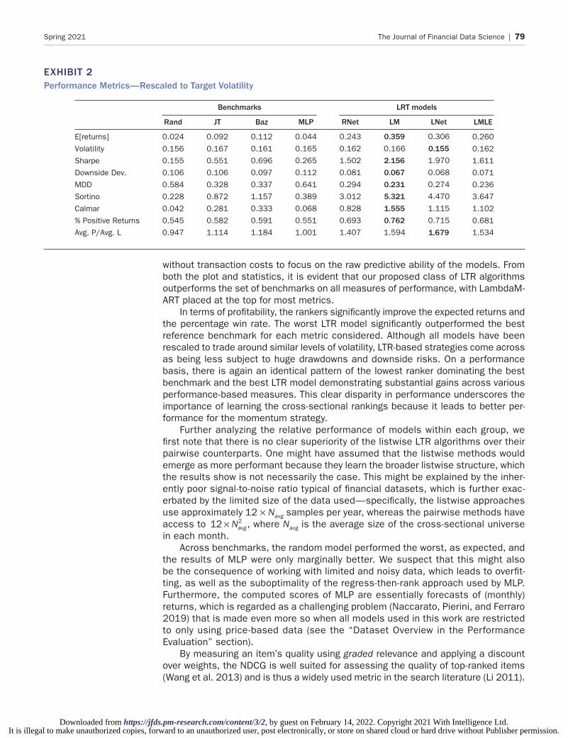
To study the out-of-sample performance across various strategies, we chart their cumulative returns in Exhibit 1 and tabulate key measures of financial performance in Exhibit 2. To allow for better comparability of strategy performance, we also apply an additional layer of volatility scaling at the portfolio level, bringing overall returns for each strategy in line with our 15% target. All returns in this section are computed

EXHIBIT 1Cumulative Returns—Rescaled to Target Volatility

104

103

102

101

100

1992 1996 2000 2004

Time

Cum

ulat

ive

Ret

urns

(log

-sca

le)

2008 2012 2016 2020

Rand JT Baz MLP

RNet LM LNet LMLE



without transaction costs to focus on the raw predictive ability of the models. From both the plot and statistics, it is evident that our proposed class of LTR algorithms outperforms the set of benchmarks on all measures of performance, with LambdaM-ART placed at the top for most metrics.

In terms of profitability, the rankers significantly improve the expected returns and the percentage win rate. The worst LTR model significantly outperformed the best reference benchmark for each metric considered. Although all models have been rescaled to trade around similar levels of volatility, LTR-based strategies come across as being less subject to huge drawdowns and downside risks. On a performance basis, there is again an identical pattern of the lowest ranker dominating the best benchmark and the best LTR model demonstrating substantial gains across various performance-based measures. This clear disparity in performance underscores the importance of learning the cross-sectional rankings because it leads to better per-formance for the momentum strategy.

Further analyzing the relative performance of models within each group, we first note that there is no clear superiority of the listwise LTR algorithms over their pairwise counterparts. One might have assumed that the listwise methods would emerge as more performant because they learn the broader listwise structure, which the results show is not necessarily the case. This might be explained by the inher-ently poor signal-to-noise ratio typical of financial datasets, which is further exac-erbated by the limited size of the data used—specifically, the listwise approaches use approximately 12 × Navg samples per year, whereas the pairwise methods have access to × Navg12 2 , where Navg is the average size of the cross-sectional universe in each month.

Across benchmarks, the random model performed the worst, as expected, and the results of MLP were only marginally better. We suspect that this might also be the consequence of working with limited and noisy data, which leads to overfit-ting, as well as the suboptimality of the regress-then-rank approach used by MLP. Furthermore, the computed scores of MLP are essentially forecasts of (monthly) returns, which is regarded as a challenging problem (Naccarato, Pierini, and Ferraro 2019) that is made even more so when all models used in this work are restricted to only using price-based data (see the “Dataset Overview in the Performance Evaluation” section).

By measuring an item’s quality using graded relevance and applying a discount over weights, the NDCG is well suited for assessing the quality of top-ranked items (Wang et al. 2013) and is thus a widely used metric in the search literature (Li 2011).

EXHIBIT 2Performance Metrics—Rescaled to Target Volatility

Benchmarks LRT models

E[returns]

Volatility

Sharpe

Downside Dev.

MDD

Sortino

Calmar

% Positive Returns

Avg. P/Avg. L

Rand

0.024

0.156

0.155

0.106

0.584

0.228

0.042

0.545

0.947

JT

0.092

0.167

0.551

0.106

0.328

0.872

0.281

0.582

1.114

Baz

0.112

0.161

0.696

0.097

0.337

1.157

0.333

0.591

1.184

MLP

0.044

0.165

0.265

0.112

0.641

0.389

0.068

0.551

1.001

RNet

0.243

0.162

1.502

0.081

0.294

3.012

0.828

0.693

1.407

LM

0.3590.166

2.1560.0670.2315.3211.5550.7621.594

LNet

0.306

0.1551.970

0.068

0.274

4.470

1.115

0.715

1.679

LMLE

0.260

0.162

1.611

0.071

0.236

3.647

1.102

0.681

1.534



The NDCG is particularly appropriate for the CSM strategy because it determines the extent to which models are able to accurately rank stocks by profitability; using a model that is able to rank in a more precise manner makes it likelier that top-ranked assets will be selected for inclusion in the respective long–short portfolio. Given this, we assess all models based on the NDCG and set the cutoff k = 100 to match the size of each of our long–short1 portfolios. From the set of compiled rank-ing metrics that is averaged across all months in Exhibit 3, all LTR models surpass the benchmarks when measured using NDCG@100, thus highlighting their ability to produce rankings that are more accurate, leading to better out-of-sample portfolio performance. With Kendall’s Tau (rank correlation coefficient), we also see the same pattern of outperformance, noting that this time ranking quality is assessed across the entire list of assets.

To further examine how rankings quality is linked to out-of-sample results, we con-struct long-only decile portfolios: At each month, these are formed by partitioning the asset universe into equally weighted deciles based on the signals/scores produced by their respective models. For instance, assets in the top (long) decile for MLP would contain the highest 10%2 of the model’s predictions. Returns are computed similarly to Equation 1 but with a decile membership indicator τD i

m

( ) used in place of τX i

m

( ) :

rn

D rDEC i

i

ntgti

i

m m

m

m

m

m

m m

1,,

( )

1( ) ,

( )

1 1∑=σστ τ

ττ

= ττ τ+

τ

+ (12)

where =τD i

m0,1( ) and takes the value of 1 for the decile of interest and 0 otherwise.

We also perform an additional level of scaling at the portfolio level. Referring to the summary results (Exhibit 4), there is a general trend of returns and Sharpe ratios increasing from decile 1 to decile 10 across all strategies except random, which emphasizes the consistency of the momentum factor. More important is the steeper rise of these figures for the LTR models, stemming from their ability to place assets in their appropriate deciles with a greater degree of precision—leading to a greater difference in returns between the decile 1 and decile 10 portfolios. The plot of decile portfolio returns across strategies (Exhibit 5) reinforces this observation, illustrating the connection between the model’s ranking ability and the dispersion across return streams. This relationship is most pronounced for the group of LTR models, which echoes the preceding statistics, thus validating our hypothesis that better asset rankings improve strategy performance.

1 To compute NDCG for shorts, we reversed our relevance scores, which allows the most negative returns to attain the highest scores.

2 This differs from our earlier approach of using 100 instruments for each long and short portfolio at all times.

EXHIBIT 3Ranking Metrics—Average over All Rebalancing Months

Benchmarks LTR Models

Kendall’s TauNDCG@100 (longs)NDCG@100 (shorts)

Rand

0.0000.5490.552

JT

0.0160.5550.562

Baz

0.0130.5620.555

MLP

0.0080.5500.564

RNet

0.0320.5760.575

LM

0.0320.5760.585

LNet

0.0330.5780.579

LMLE

0.0200.5650.567



CONCLUSIONS

Focusing on CSM as a demonstrative use case, we introduce LTR algorithms as a novel way of ranking assets, which is an important step required by cross-sec-tional systematic strategies. Additionally, the modular framework underpinning these algorithms allows additional feature inputs to be flexibly incorporated, thus providing a generalizable platform for a broader set of cross-sectional strategies. In learning the relational (pairwise or listwise) structure across assets that both heuristics and regress-then-rank approaches only superficially capture, we obtain a more accu-rate ranking across instruments. This translates to Sharpe ratios being boosted approximately threefold over traditional approaches and provides clear and significant improvements in both performance and ranking quality–related measures.

Some directions for future work include innovating in terms of architecture or model ensembling to further improve strategy performance, as well as studying the effectiveness of these ranking techniques on higher-frequency data (e.g., order book) and asset classes.

EXHIBIT 4Performance Metrics—Decile Portfolios Rescaled to Target Volatility

Decile

RandE[returns]VolatilitySharpe

JTE[returns]VolatilitySharpe

BazE[returns]VolatilitySharpe

MLPE[returns]VolatilitySharpe

RNetE[returns]VolatilitySharpe

LME[returns]Volatility

LMLEE[returns]VolatilitySharpe

1

0.1100.1620.675

0.0590.1650.360

0.0950.1630.582

0.0720.1630.443

0.0430.1640.263

0.0120.161

0.0590.1650.360

2

0.1200.1630.737

0.0710.1640.435

0.0940.1630.573

0.1120.1610.697

0.0670.1640.405

0.0740.165

0.0800.1640.489

3

0.1180.1640.721

0.0960.1650.581

0.0830.1620.510

0.1220.1630.751

0.0790.1640.480

0.0970.162

0.0880.1640.537

4

0.1240.1620.769

0.1080.1640.661

0.0940.1620.579

0.1140.1620.703

0.0950.1640.580

0.0980.163

0.1100.1650.671

5

0.1140.1640.697

0.1220.1630.746

0.0920.1630.566

0.1270.1630.780

0.1150.1640.698

0.1170.164

0.1090.1610.677

6

0.1230.1620.763

0.1270.1630.780

0.1090.1620.671

0.1260.1620.779

0.1210.1630.742

0.1320.162

0.1230.1640.750

7

0.1260.1630.772

0.1370.1630.840

0.1240.1620.765

0.1300.1630.800

0.1400.1610.870

0.1310.164

0.1260.1620.782

8

0.1150.1610.710

0.1510.1620.928

0.1370.1620.849

0.1350.1630.825

0.1470.1620.906

0.1410.162

0.1510.1610.937

9

0.1260.1630.772

0.1460.1600.910

0.1600.1630.984

0.1240.1630.758

0.1630.1611.014

0.1710.163

0.1630.1601.016

10

0.1150.1640.702

0.1460.1560.938

0.1850.1631.130

0.1320.1640.806

0.2020.1631.238

0.2010.162

0.1930.1631.186

L–S

0.0280.1560.177

0.0940.1670.565

0.1070.1610.664

0.0970.1680.578

0.2460.1611.527

0.3490.155

0.2440.1601.530

Sharpe 0.075 0.449 0.599 0.606 0.716 0.806 0.800 0.868 1.053 1.232 2.107

LNetE[returns] 0.037 0.069 0.089 0.102 0.116 0.117 0.137 0.152 0.151 0.186 0.296Volatility 0.161 0.165 0.162 0.163 0.164 0.162 0.164 0.162 0.163 0.162 0.155Sharpe 0.232 0.416 0.549 0.628 0.711 0.720 0.837 0.938 0.929 1.148 1.911



APPENDIX

LEARNING TO RANK FOR CROSS-SECTIONAL MOMENTUM

LTR is a supervised learning task involving training and testing phases. Document retrieval is the standard problem setting to make specific the LTR framework, and we follow this convention. For training, we are provided with a set of queries Q = q1, …, qm. Each query qi has an associated list of documents =d d di i i

ni , ..., (1) ( ) , where ni is the total number of documents for qi, and an accompanying set of document labels

=y y yi i ini , ..., (1) ( ) , where the labels represent grades. Letting Y = Y1, …, Yℓ be the label

set, we have Y∈yij( ) for ∀ i, j. We also have Yℓ Yℓ-1 … Y1 , where stands for

the order relation—a higher grade on a given document implies a stronger relevance of the document with respect to its query. For each query–document pair, a feature vector

= φx q dij

i ij( , )( ) ( ) can be formed, noting that f(·) is a feature function, i ∈ 1, …, m and j ∈

1, …, ni. Letting =x x xini , ..., (1) ( ) , we can assemble the training set =x yi i i

m , 1. The goal of LTR is to learn a function f that predicts a score =+ +f x zm

imi( )1

( )1

( ) when presented with an out-of-sample input +xm

i1

( ) . For more details, we point the reader to Li (2011).Transposing the preceding framework to the momentum strategy, we can treat each

query as being analogous to a portfolio rebalancing event, whereas an associated doc-ument and its accompanying label can be thought of, respectively, as an asset and its assigned decile at the next rebalance based on some performance measure (convention-ally taken to be returns). Exhibit A1 provides a schematic of this adaptation, which we further make concrete. For training, let B = b1, …, bm-1 be a series of monthly rebalances in which at each bi we have a set of equity instruments , ..., (1) ( )=e e ei i i

ni and the set of assigned deciles , ..., 1 1

(1)1

( )δδ = δ δ+ + +i i ini , where D D Dδ ∈ =+i

j , ..., 1( )

1 10 for ∀ i, j. Similar

to earlier, k > l ⇒ Dk Dl for k, l ∈ 1, …, 10. With each rebalance–asset pair, we can form the feature vector = φu b ei

ji i

j( , )( ) ( ) and the broader training set , 1 11δδ + =

−ui i im , where

=u u ui i ini , ..., (1) ( ) . Note that other features can be incorporated for ui

j( ), allowing different types of cross-sectional strategies to be developed. Presented with sets of feature vec-tors for testing at interval m with a trained function g produced by the learning system,

EXHIBIT 5Cumulative Returns—Decile Portfolios Rescaled to Target Volatility

JT

LM

Baz

LNet

MLP

LMLE

Rand

102

101

100

RNet

102

101

100

Cum

ulat

ive

Ret

urns

(log

-sca

le)

1995

2000

2005

2010

2015

2020

1995

2000

2005

2010

2015

2020

1995

2000

2005

2010

2015

2020

1995

2000

2005

2010

2015

2020

1 2 3 4 5 6 7 8 9 10



we compute the set of scores ug m( ) in the score calculation phase and then go on to form the long–short portfolios by following the instructions described in the “Strategy Framework” under the section on “Problem Definition.”

ADDITIONAL TRAINING DETAILS

Python libraries: LambdaMART uses XGBoost (Chen and Guestrin 2016), and the oth-ers—RankNet, ListNet, and ListMLE—are developed using TensorFlow (Abadi et al. 2015).

Hyperparameter optimization: Hyperparameters assume discrete values and are tuned using HyperOpt (Bergstra et al. 2015). For LambdaMART, we refer to the hyperpa-rameters as they are named in the XGBoost library.

Multilayer perceptron (MLP):

§Dropout rate: [0.0, 0.2, 0.4, 0.6, 0.8]§Hidden width: [64, 128, 256, 512, 1024, 2048]§Max gradient norm: [10–3, 10–2, 10–1, 1, 10]§Learning rate: [10–6, 10–5, 10–4, 10–3, 10–2, 10–1, 1]§Minibatch size: [64, 128, 256, 512, 1024]

RankNet:

§Dropout rate: [0.0, 0.2, 0.4, 0.6, 0.8]§Hidden width: [64, 128, 256, 512, 1024, 2048]§Max gradient norm: [10–3, 10–2, 10–1, 1, 10]§Learning rate: [10–6, 10–5, 10–4, 10–3, 10–2, 10–1, 1]§Securities used to form pairs for minibatch: [64, 128, 256, 512, 1024]

LambdaMART:

§objective: rank:pairwise§eval_metric: ndcg§eta: [10–6, 10–5, 10–4, 10–3, 10–2, 10–1, 1]§num_boost_round: [5, 10, 20, 40, 80, 160, 320]

EXHIBIT A1Learning to Rank for Cross-Sectional Momentum

ScoreCalculation

LearningSystem

ScoreRanking

SecuritySelection

PortfolioConstruction

bm

em

(nm)e

mem

(1),•••,=

•••

g(um )(1)

g(um

)(nm)

em(1)

•••

em

(nm)

e1(1)

e1

(n1)

•••

em–1(1)

em–1

(nm–1)

•••

b1 bm–1

,•••,

g(•)

Zm

Xm

Training Data Out-of-Sample Data



§max_depth: [2, 4, 6, 8, 10]§tree_method: gpu_hist

ListMLE, ListNet:

§Dropout rate: [0.0, 0.2, 0.4, 0.6, 0.8]§Hidden width: [64, 128, 256, 512, 1024, 2048]§Max gradient norm: [10–3, 10–2, 10–1, 1, 10]§Learning rate: [10–8, 10–7, 10–6, 10–5, 10–4]§Minibatch size: [1, 2, 4, 8, 16]

REFERENCES

Abadi, M., A. Agarwal, P. Barham, E. Brevdo, Z. Chen, C. Citro, G. S. Corrado, A. Davis, J. Dean, M. Devin, S. Ghemawat, I. Goodfellow, A. Harp, G. Irving, M. Isard, Y. Jia, R. Jozefowicz, L. Kaiser, M. Kudlur, J. Levenberg, D. Mané, R. Monga, S. Moore, D. Murray, C. Olah, M. Schuster, J. Shlens, B. Steiner, I. Sutskever, K. Talwar, P. Tucker, V. Vanhoucke, V. Vasudevan, F. Viégas, O. Vinyals, P. Warden, M. Wattenberg, M. Wicke, Y. Yu, and X. Zheng. “TensorFlow: Large-Scale Machine Learning on Heterogeneous Systems.” 2015. https://www.tensorflow.org.

Baz, J., N. M. Granger, C. R. Harvey, N. Le Roux, and S. Rattray. 2015. “Dissecting Investment Strategies in the Cross Section and Time Series.” SSRN Electronic Journal. Available at SSRN: https://ssrn.com/abstract=2695101 or http://dx.doi.org/10.2139/ssrn.2695101.

Bergstra, J., B. Komer, C. Eliasmith, D. Yamins, and D. D. Cox. 2015. “Hyperopt: A Python Library for Model Selection and Hyperparameter Optimization.” Computational Science & Discovery 8 (1): 014008.

Bollerslev, T. 1986. “Generalized Autoregressive Conditional Heteroskedasticity.” Journal of Econo-metrics 31 (3): 307–327.

Boyd, S., and L. Vandenberghe. 2004. Convex Optimization. USA: Cambridge University Press.

Bruch, S. 2020. “An Alternative Cross Entropy Loss for Learning-to-Rank.” arXiv:1911.09798, 2020.

Burges, C. “From RankNet to LambdaRank to LambdaMART: An Overview.” Microsoft Research, Technical report MSR-TR-2010-82, 2010.

Burges, C., R. Ragno, and Q. Le. 2006. “Learning to Rank with Nonsmooth Cost Functions.” Pro-ceedings of the 19th International Conference on Neural Information Processing Systems. NIPS’06, 193–200. Cambridge, MA: MIT Press, 2006.

Burges, C., T. Shaked, E. Renshaw, A. Lazier, M. Deeds, N. Hamilton, and G. Hullender. “Learning to Rank Using Gradient Descent.” Proceedings of the 22nd International Conference on Machine Learning. ICML ’05, 89–96. New York: Association for Computing Machinery, 2005.

Cao, Z., T. Qin, T.-Y. Liu, M.-F. Tsai, and H. Li. 2007. “Learning to Rank: From Pairwise Approach to Listwise Approach.” Proceedings of the 24th International Conference on Machine Learning—ICML ’07, 129–136. Corvalis, OR: ACM Press, 2007.

Center for Research in Security Prices (CRSP), The University of Chicago Booth School of Business. “NYSE Equity Data from 1980 to 2019.” Calculated (or derived) based on data from CRSP Daily Stock, 2019.

Chen, T., and C. Guestrin. “XGBoost: A Scalable Tree Boosting System.” Proceedings of the 22nd ACM SIGKDD International Conference on Knowledge Discovery and Data Mining. KDD ’16, 785–794. New York: Association for Computing Machinery, 2016.


https://www.tensorflow.org

https://ssrn.com/abstract=2695101

http://dx.doi.org/10.2139/ssrn.2695101


Chui, A. C. W., S. Titman, and K. C. J. Wei. 2010. “Individualism and Momentum around the World.” The Journal of Finance 65 (1): 361–392.

de Groot, W., J. Pang, and L. Swinkels. 2012. “The Cross-Section of Stock Returns in Frontier Emerging Markets.” Journal of Empirical Finance 19 (5): 796–818.

Donmez, P., K. M. Svore, and C. Burges. “On the Local Optimality of LambdaRank.” Proceedings of the 32nd International ACM SIGIR Conference on Research and Development in Information Retrieval—SIGIR ’09, 460–467. Boston: ACM Press, 2009.

Erb, C. B., and C. R. Harvey. 2006. “The Strategic and Tactical Value of Commodity Futures.” Financial Analysts Journal 62 (2): 69–97.

Griffin, J. M., X. Ji, and J. S. Martin. 2003. “Momentum Investing and Business Cycle Risk: Evidence from Pole to Pole.” The Journal of Finance 58 (6): 2515–2547.

Gu, S., B. Kelly, and D. Xiu. Empirical Asset Pricing via Machine Learning. Technical report w25398, National Bureau of Economic Research, 2018.

——. “Autoencoder Asset Pricing Models.” Yale ICF Working Paper No. 2019-04, Chicago Booth Research Paper No. 19-24, 2019. https://ssrn.com/abstract=3335536.

Järvelin, K., and J. Kekäläinen. “IR Evaluation Methods for Retrieving Highly Relevant Documents.” Proceedings of the 23rd Annual International ACM SIGIR Conference on Research and Development in Information Retrieval—SIGIR ’00, 41–48. Athens, Greece: ACM Press, 2000.

Jegadeesh, N., and S. Titman. 1993. “Returns to Buying Winners and Selling Losers: Implications for Stock Market Efficiency.” The Journal of Finance 48 (1): 65–91.

Jusselin, P., E. Lezmi, H. Malongo, C. Masselin, T. Roncalli, and T.-L. Dao. “Understanding the Momentum Risk Premium: An In-Depth Journey through Trend-Following Strategies.” SSRN Elec-tronic Journal, 2017. https://ssrn.com/abstract=3042173.

Kim, S. 2019. “Enhancing the Momentum Strategy through Deep Regression.” Quantitative Finance 19 (7): 1121–1133.

LeBaron, B. Technical Trading Rule Profitability and Foreign Exchange Intervention. Technical report w5505, National Bureau of Economic Research, 1996.

Li, H. 2011. “Learning to Rank for Information Retrieval and Natural Language Processing.” Syn-thesis Lectures on Human Language Technologies 4 (1): 1–113.

Li, P., Z. Qin, X. Wang, and D. Metzler. “Combining Decision Trees and Neural Networks for Learn-ing-to-Rank in Personal Search.” Proceedings of the 25th ACM SIGKDD International Conference on Knowledge Discovery & Data Mining, 2032–2040. Anchorage, AK: Association for Computing Machinery, 2019.

Lim, B., S. Zohren, and S. Roberts. “Enhancing Time Series Momentum Strategies Using Deep Neural Networks.” SSRN Electronic Journal, 2019. https://ssrn.com/abstract=3369195.

Liu, T.-Y. Learning to Rank for Information Retrieval. Berlin, Germany: Springer, 2011.

Moskowitz, T. J., Y. H. Ooi, and L. H. Pedersen. 2012. “Time Series Momentum.” Journal of Finan-cial Economics 104 (2): 228–250.

Naccarato, A., A. Pierini, and G. Ferraro. 2019. “Markowitz Portfolio Optimization through Pairs Trad-ing Cointegrated Strategy in Long-Term Investment.” Annals of Operations Research 276 (1–2): 1–19.

Nguyen, P., J. Wang, and A. Kalousis. 2016. “Factorizing LambdaMART for Cold Start Recommen-dations.” Machine Learning 104 (2): 223–242.

Pasumarthi, R. K., S. Bruch, X. Wang, C. Li, M. Bendersky, M. Najork, J. Pfeifer, N. Golbandi, R. Anil, and S. Wolf. “TF-Ranking: Scalable TensorFlow Library for Learning-to-Rank.” Proceed-ings of the 25th ACM SIGKDD International Conference on Knowledge Discovery & Data Mining, 2970–2978. Anchorage, AK: Association for Computing Machinery, 2019.






Paszke, A., S. Gross, F. Massa, A. Lerer, J. Bradbury, G. Chanan, T. Killeen, Z. Lin, N. Gimelshein, L. Antiga, A. Desmaison, A. Kopf, E. Yang, Z. DeVito, M. Raison, A. Tejani, S. Chilamkurthy, B. Steiner, L. Fang, J. Bai, and S. Chintala. “PyTorch: An Imperative Style, High-Performance Deep Learning Library.” In Advances in Neural Information Processing Systems 32, edited by H. Wallach, H. Larochelle, A. Beygelzimer, F. dAlché-Buc, E. Fox, and R. Garnett, 8024–8035. Lake Tahoe, NV: Curran Associates, 2019.

Pereira, B. L., A. Ueda, G. Penha, R. L. T. Santos, and N. Ziviani. 2019. “Online Learning to Rank for Sequential Music Recommendation.” Proceedings of the 13th ACM Conference on Recommender Systems, 237–245. Copenhagen, Denmark: Association for Computing Machinery.

Pirrong, C. 2005. “Momentum in Futures Markets.” SSRN Electronic Journal, 2005.

Rohrbach, J., and S. Suremann. 2017. “Momentum in Traditional and Cryptocurrencies Made Simple.” SSRN Electronic Journal, 2017.

Roncalli, T. 2017. “Keep Up the Momentum.” SSRN Electronic Journal, 2017. https://ssrn.com/abstract=3751012.

Rouwenhorst, K. G. 1998. “International Momentum Strategies.” The Journal of Finance 53 (1): 267–284.

Santu, S. K. K., P. Sondhi, and C.-X. Zhai. 2017. “On Application of Learning to Rank for E-Commerce Search.” Proceedings of the 40th International ACM SIGIR Conference on Research and Development in Information Retrieval, 475–484.

Song, Q., A. Liu, and S. Y. Yang. 2017. “Stock Portfolio Selection Using Learning-to-Rank Algorithms with News Sentiment.” Neurocomputing 264 (November): 20–28.

Srivastava, N., G. Hinton, A. Krizhevsky, I. Sutskever, and R. Salakhutdinov. 2014. “Dropout: A Simple Way to Prevent Neural Networks from Overfitting.” Journal of Machine Learning Research 15 (56): 1929–1958.

Wang, B., and D. Klabjan. 2017. “An Attention-Based Deep Net for Learning to Rank.” 2017. arXiv:1702.06106 [cs].

Wang, L., and K. Rasheed. “Stock Ranking with Market Microstructure, Technical Indicator and News.” Proceedings on the International Conference on Artificial Intelligence (ICAI), 322–328. New York: Springer, 2018.

Wang, P., C. Liu, Y. Yang, and S. Huang. “A Robo-Advisor Design Using Multiobjective Rank-nets with Gated Neural Network Structure.” 2019 IEEE International Conference on Agents (ICA), 77–78. Piscataway, NJ: IEEE, 2019.

Wang, Y., L. Wang, Y. Li, D. He, and T.-Y. Liu. “A Theoretical Analysis of NDCG Type Ranking Mea-sures.” 26th Annual Conference on Learning Theory. Proceedings of Machine Learning Research, vol. 30, edited by S. Shalev-Shwartz and I. Steinwart, 25–54. Princeton, NJ: PMLR, 2013.

Wu, Q., C. Burges, K. M. Svore, and J. Gao. 2010. “Adapting Boosting for Information Retrieval Measures.” Information Retrieval 13 (3): 254–270.

Xia, F., T.-Y. Liu, J. Wang, W. Zhang, and H. Li. 2008. “Listwise Approach to Learning to Rank: Theory and Algorithm.” Proceedings of the 25th International Conference on Machine Learning. ICML ’08, 1192–1199. New York: Association for Computing Machinery.

Yue, Y., and C. Burges. “On Using Simultaneous Perturbation Stochastic Approximation for Learn-ing to Rank, and the Empirical Optimality of LambdaRank.” Microsoft Research, Technical report MSR-TR-2007-115, 2007.

To order reprints of this article, please contact David Rowe at [email protected] or 646-891-2157.




Building Cross-Sectional Systematic Strategies by Learning ...

Documents

Transcript of Building Cross-Sectional Systematic Strategies by Learning ...