1

CROSS-SECTIONAL MIXTURE MODELINGShaunna L. ClarkAdvanced Genetic Epidemiology Statistical WorkshopOctober 23, 2012

2

OUTLINE What is a mixture? Introduction to LCA (LPA)

Basic Analysis Ideas\Plan and Issues How to choose the number of classes

How do we implement mixtures in OpenMx? Factor Mixture Model What do classes mean for twin modeling?

3

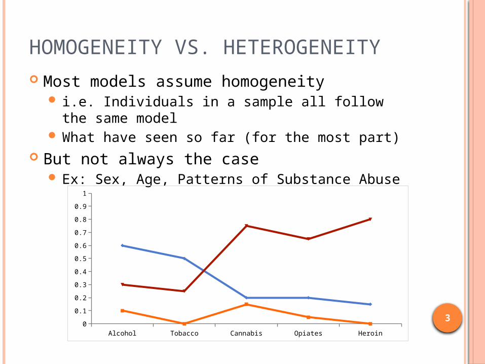
HOMOGENEITY VS. HETEROGENEITY Most models assume homogeneity

i.e. Individuals in a sample all follow the same model

What have seen so far (for the most part) But not always the case

Ex: Sex, Age, Patterns of Substance Abuse

Alcohol Tobacco Cannabis Opiates Heroin0

0.10.20.30.40.50.60.70.80.9

1

4

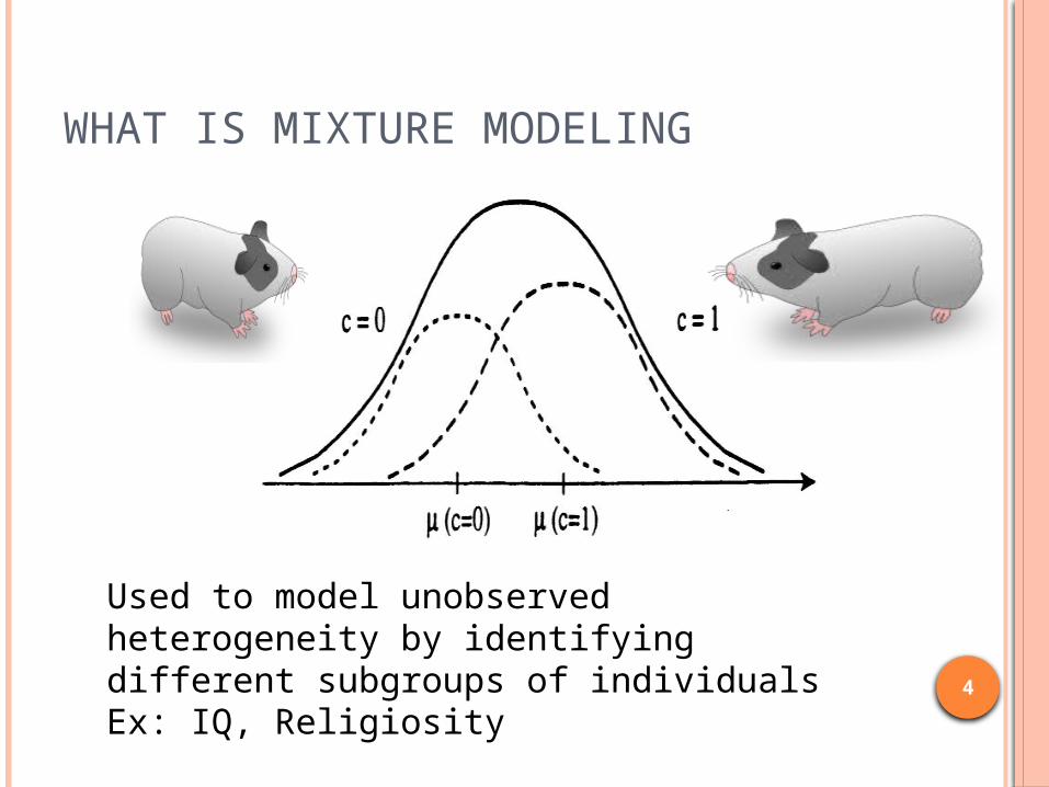
WHAT IS MIXTURE MODELING

Used to model unobserved heterogeneity by identifying different subgroups of individuals

Ex: IQ, Religiosity

5

LATENT CLASS ANALYSIS (LCA)Also known as Latent Profile Analysis (LPA) if you have continuously distributed variables

6

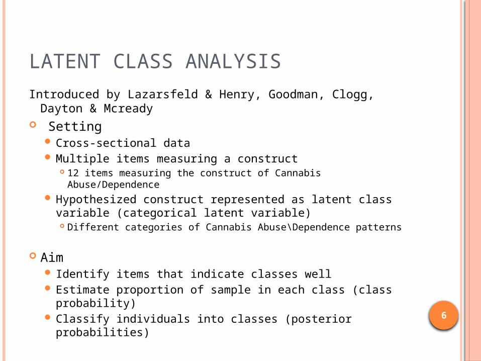
LATENT CLASS ANALYSISIntroduced by Lazarsfeld & Henry, Goodman, Clogg, Dayton

& Mcready Setting

Cross-sectional data Multiple items measuring a construct

12 items measuring the construct of Cannabis Abuse/Dependence Hypothesized construct represented as latent class

variable (categorical latent variable) Different categories of Cannabis Abuse\Dependence patterns

Aim Identify items that indicate classes well Estimate proportion of sample in each class (class

probability) Classify individuals into classes (posterior probabilities)

7

LATENT CLASS ANALYSIS CONT’D

x1 x2 x3 x4 x5

C

Alcohol Tobacco Cannabis Opiates Heroin0

0.1

0.2

0.3

0.4

0.5

0.6

0.7

0.8

0.9

1

Non UsersLegal Drug UsersMultiple Illicit Users

8

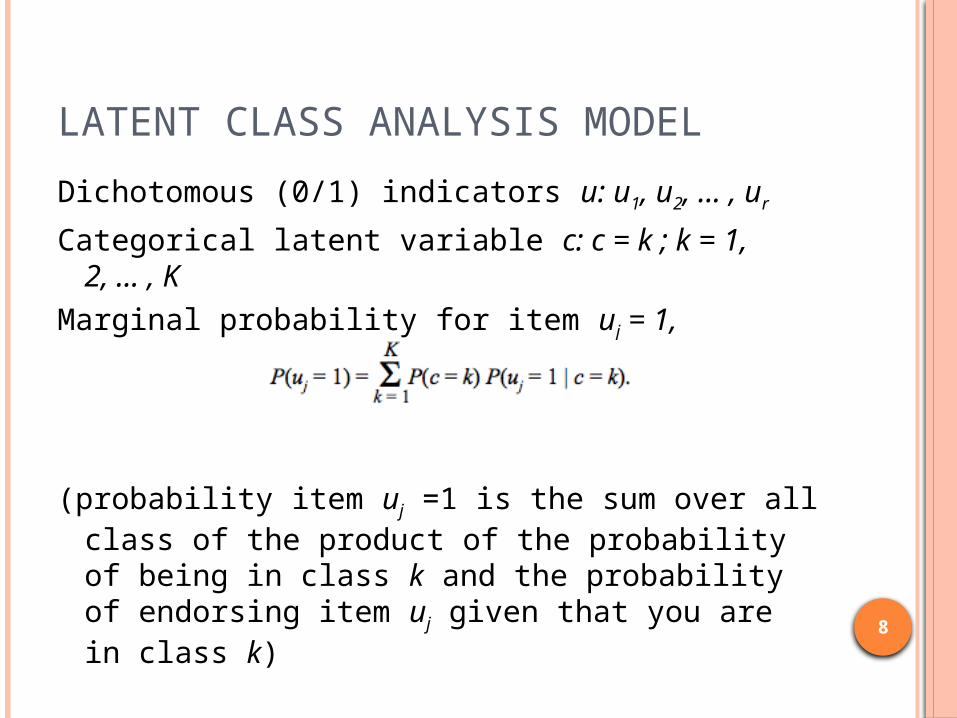
LATENT CLASS ANALYSIS MODELDichotomous (0/1) indicators u: u1, u2, ... , ur

Categorical latent variable c: c = k ; k = 1, 2, ... , K

Marginal probability for item uj = 1,

(probability item uj =1 is the sum over all class of the product of the probability of being in class k and the probability of endorsing item uj given that you are in class k)

9

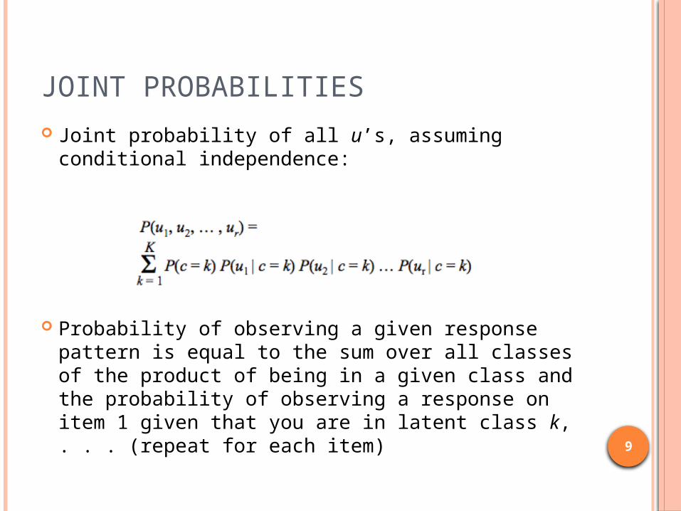
JOINT PROBABILITIES Joint probability of all u’s, assuming conditional

independence:

Probability of observing a given response pattern is equal to the sum over all classes of the product of being in a given class and the probability of observing a response on item 1 given that you are in latent class k, . . . (repeat for each item)

10

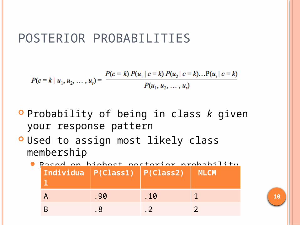
POSTERIOR PROBABILITIES

Probability of being in class k given your response pattern

Used to assign most likely class membership Based on highest posterior probability

Individual P(Class1) P(Class2) MLCMA .90 .10 1B .8 .2 2

11

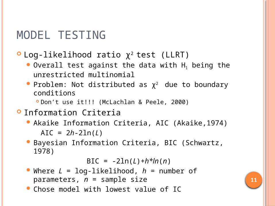
MODEL TESTING Log-likelihood ratio χ2 test (LLRT)

Overall test against the data with H1 being the unrestricted multinomial

Problem: Not distributed as χ2 due to boundary conditions Don’t use it!!! (McLachlan & Peele, 2000)

Information Criteria Akaike Information Criteria, AIC (Akaike,1974)

AIC = 2h-2ln(L) Bayesian Information Criteria, BIC (Schwartz, 1978)

BIC = -2ln(L)+h*ln(n) Where L = log-likelihood, h = number of parameters,

n = sample size Chose model with lowest value of IC

12

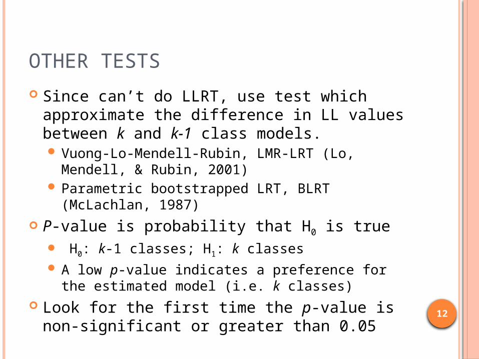
OTHER TESTS Since can’t do LLRT, use test which

approximate the difference in LL values between k and k-1 class models. Vuong-Lo-Mendell-Rubin, LMR-LRT (Lo, Mendell, &

Rubin, 2001) Parametric bootstrapped LRT, BLRT (McLachlan,

1987) P-value is probability that H0 is true

H0: k-1 classes; H1: k classes A low p-value indicates a preference for the

estimated model (i.e. k classes) Look for the first time the p-value is non-

significant or greater than 0.05

13

ANALYSIS PLAN1. Fit model with 1-class

Everyone in same class Sometimes simple is better

2. Fit LCA models 2-K classes3. Chose best number of classes

Seems simple right???

14

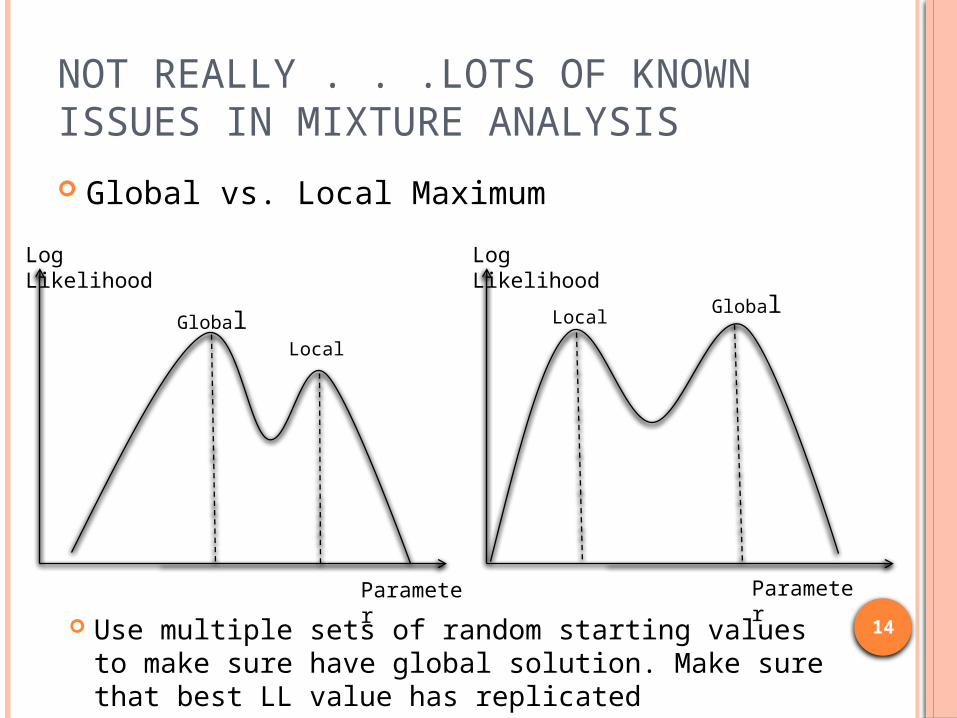
NOT REALLY . . .LOTS OF KNOWN ISSUES IN MIXTURE ANALYSIS Global vs. Local Maximum

Log Likelihood

Parameter

GlobalLocal

Log Likelihood

GlobalLocal

Use multiple sets of random starting values to make sure have global solution. Make sure that best LL value has replicated

Parameter

15

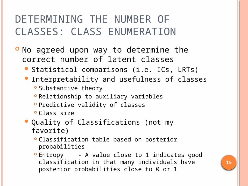
DETERMINING THE NUMBER OF CLASSES: CLASS ENUMERATION No agreed upon way to determine the correct

number of latent classes Statistical comparisons (i.e. ICs, LRTs) Interpretability and usefulness of classes

Substantive theory Relationship to auxiliary variables Predictive validity of classes Class size

Quality of Classifications (not my favorite) Classification table based on posterior probabilities Entropy - A value close to 1 indicates good

classification in that many individuals have posterior probabilities close to 0 or 1

16

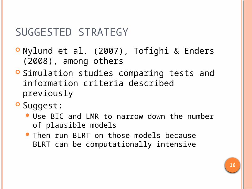
SUGGESTED STRATEGY Nylund et al. (2007), Tofighi & Enders (2008),

among others Simulation studies comparing tests and

information criteria described previously Suggest:

Use BIC and LMR to narrow down the number of plausible models

Then run BLRT on those models because BLRT can be computationally intensive

17

OPENMX: LCA EXAMPLE SCRIPTLCA_example.R

18

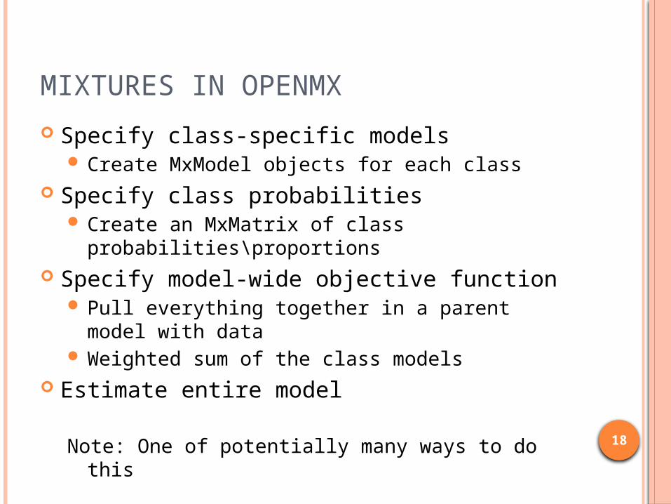
MIXTURES IN OPENMX Specify class-specific models

Create MxModel objects for each class Specify class probabilities

Create an MxMatrix of class probabilities\proportions

Specify model-wide objective function Pull everything together in a parent model with

data Weighted sum of the class models

Estimate entire model

Note: One of potentially many ways to do this

19

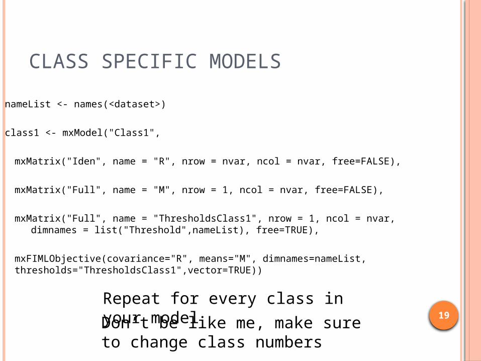
CLASS SPECIFIC MODELSnameList <- names(<dataset>)

class1 <- mxModel("Class1",

mxMatrix("Iden", name = "R", nrow = nvar, ncol = nvar, free=FALSE),

mxMatrix("Full", name = "M", nrow = 1, ncol = nvar, free=FALSE),

mxMatrix("Full", name = "ThresholdsClass1", nrow = 1, ncol = nvar, dimnames = list("Threshold",nameList), free=TRUE),

mxFIMLObjective(covariance="R", means="M", dimnames=nameList, thresholds="ThresholdsClass1",vector=TRUE))

Repeat for every class in your modelDon’t be like me, make sure to change class numbers

20

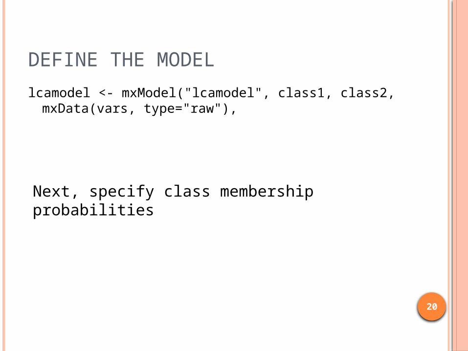
DEFINE THE MODELlcamodel <- mxModel("lcamodel", class1, class2,

mxData(vars, type="raw"),

Next, specify class membership probabilities

21

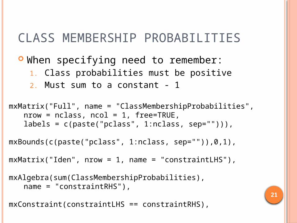
CLASS MEMBERSHIP PROBABILITIES When specifying need to remember:

1. Class probabilities must be positive2. Must sum to a constant - 1

mxMatrix("Full", name = "ClassMembershipProbabilities", nrow = nclass, ncol = 1, free=TRUE, labels = c(paste("pclass", 1:nclass, sep=""))),

mxBounds(c(paste("pclass", 1:nclass, sep="")),0,1),

mxMatrix("Iden", nrow = 1, name = "constraintLHS"),

mxAlgebra(sum(ClassMembershipProbabilities), name = "constraintRHS"),

mxConstraint(constraintLHS == constraintRHS),

22

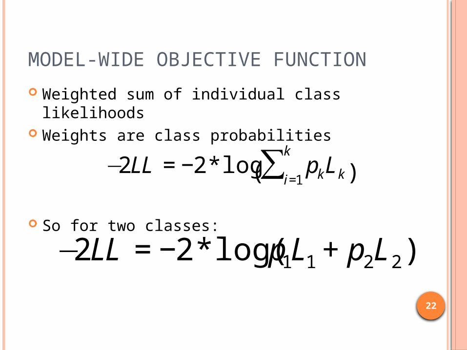
MODEL-WIDE OBJECTIVE FUNCTION Weighted sum of individual class likelihoods Weights are class probabilities

So for two classes:

€

−2LL = −2* log pkLki=1

k∑( )

€

−2LL = −2* log(p1L1 + p2L2)

23

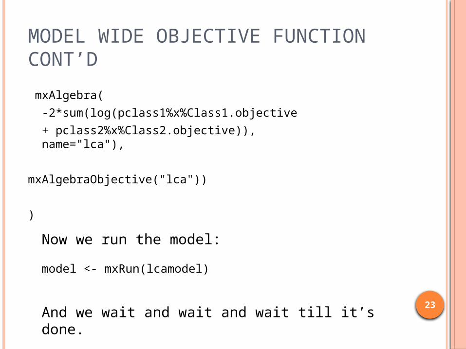
MODEL WIDE OBJECTIVE FUNCTION CONT’D mxAlgebra(

-2*sum(log(pclass1%x%Class1.objective + pclass2%x%Class2.objective)), name="lca"),

mxAlgebraObjective("lca"))

)

Now we run the model:model <- mxRun(lcamodel)

And we wait and wait and wait till it’s done.

24

PROFILE PLOT One way to interpret the classes is to plot

them. In our example we had binary items, so the

thresholds are what distinguishes between classes Can plot the thresholds

Or you can plot the probabilities More intuitive Easier for non-statisticians to understand

25

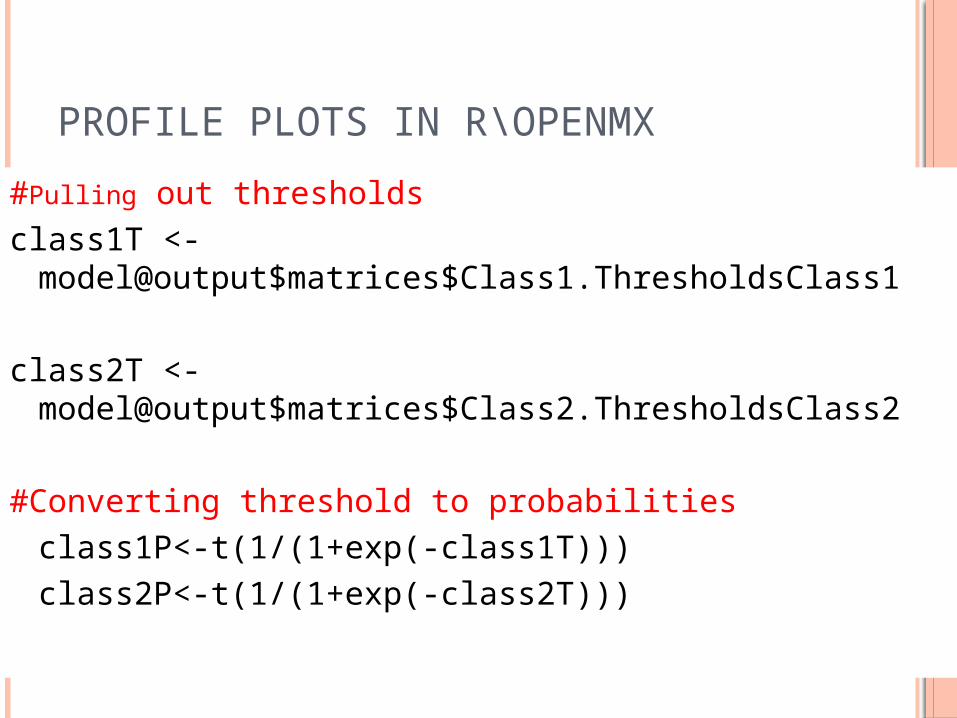
PROFILE PLOTS IN R\OPENMX#Pulling out thresholdsclass1T <-

model@output$matrices$Class1.ThresholdsClass1

class2T <- model@output$matrices$Class2.ThresholdsClass2

#Converting threshold to probabilitiesclass1P<-t(1/(1+exp(-class1T)))class2P<-t(1/(1+exp(-class2T)))

26

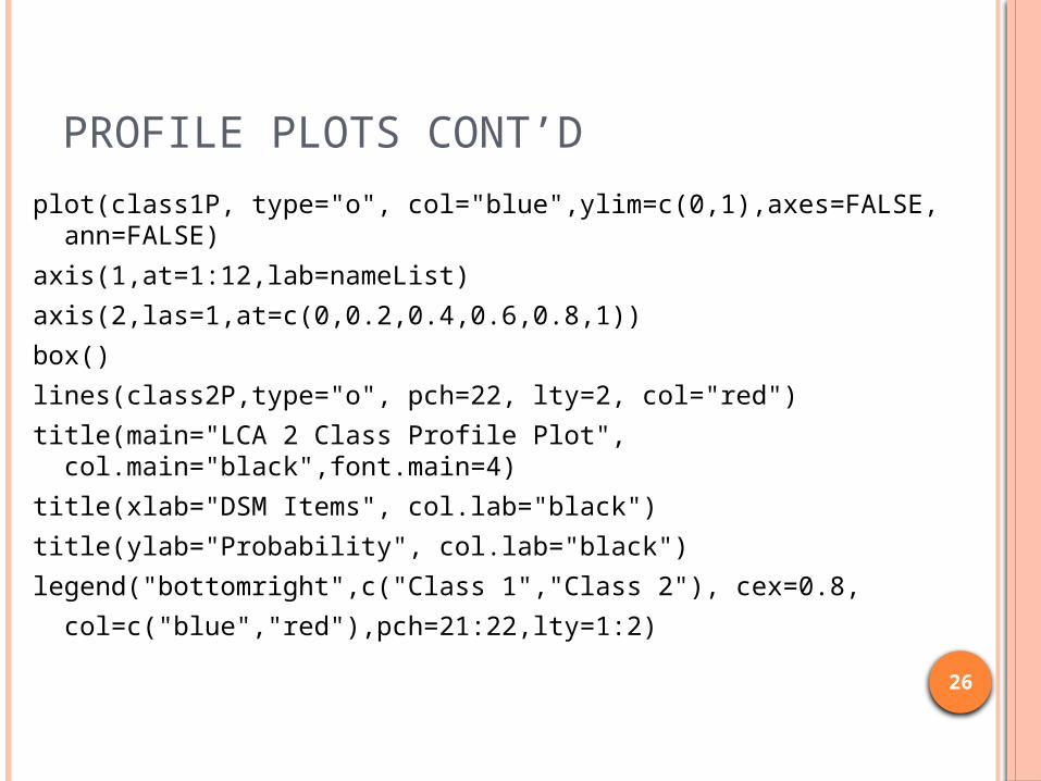
PROFILE PLOTS CONT’Dplot(class1P, type="o", col="blue",ylim=c(0,1),axes=FALSE,

ann=FALSE)axis(1,at=1:12,lab=nameList)axis(2,las=1,at=c(0,0.2,0.4,0.6,0.8,1))box()lines(class2P,type="o", pch=22, lty=2, col="red")title(main="LCA 2 Class Profile Plot", col.main="black",font.main=4)title(xlab="DSM Items", col.lab="black")title(ylab="Probability", col.lab="black")legend("bottomright",c("Class 1","Class 2"), cex=0.8,

col=c("blue","red"),pch=21:22,lty=1:2)

27

OPENMX EXERCISE Unfortunately, it takes long time for these to

run so not feasible to do in this session However, I’ve run the 2-, 3-, and 4- class LCA

models for this data and (hopefully) the .Rdata files are posted on the website

Exercise: Using the .Rdata files1. Determine which model is better according to AIC\BIC

Want the lowest value2. Make a profile plot of the best solution and interpret

the classes What kind of substances users are there?

28

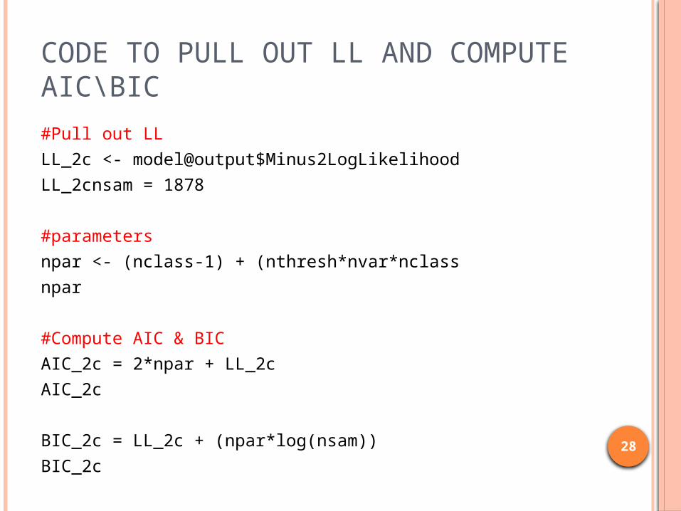
CODE TO PULL OUT LL AND COMPUTE AIC\BIC#Pull out LLLL_2c <- model@output$Minus2LogLikelihoodLL_2cnsam = 1878

#parametersnpar <- (nclass-1) + (nthresh*nvar*nclassnpar

#Compute AIC & BICAIC_2c = 2*npar + LL_2c AIC_2c

BIC_2c = LL_2c + (npar*log(nsam))BIC_2c

29

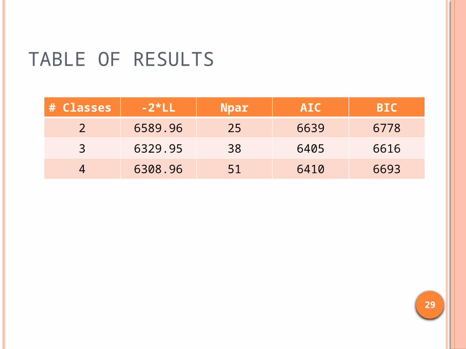
TABLE OF RESULTS

# Classes -2*LL Npar AIC BIC2 6589.96 25 6639 67783 6329.95 38 6405 66164 6308.96 51 6410 6693

30

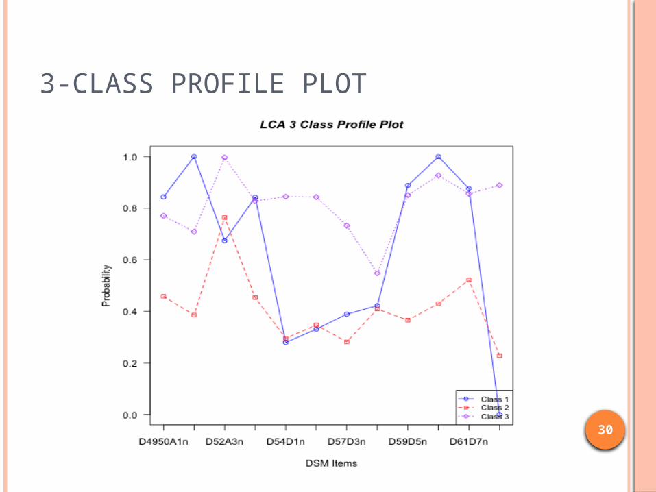
3-CLASS PROFILE PLOT

31

FACTOR MIXTURE MODELING

32

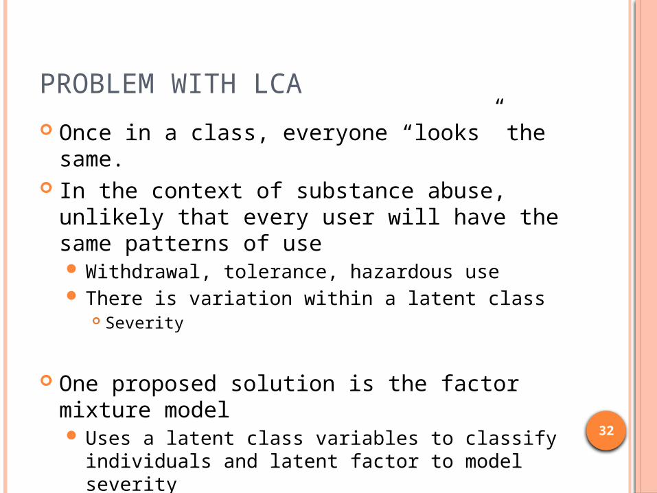
PROBLEM WITH LCA Once in a class, everyone “looks” the same. In the context of substance abuse, unlikely

that every user will have the same patterns of use Withdrawal, tolerance, hazardous use There is variation within a latent class

Severity

One proposed solution is the factor mixture model Uses a latent class variables to classify

individuals and latent factor to model severity

33

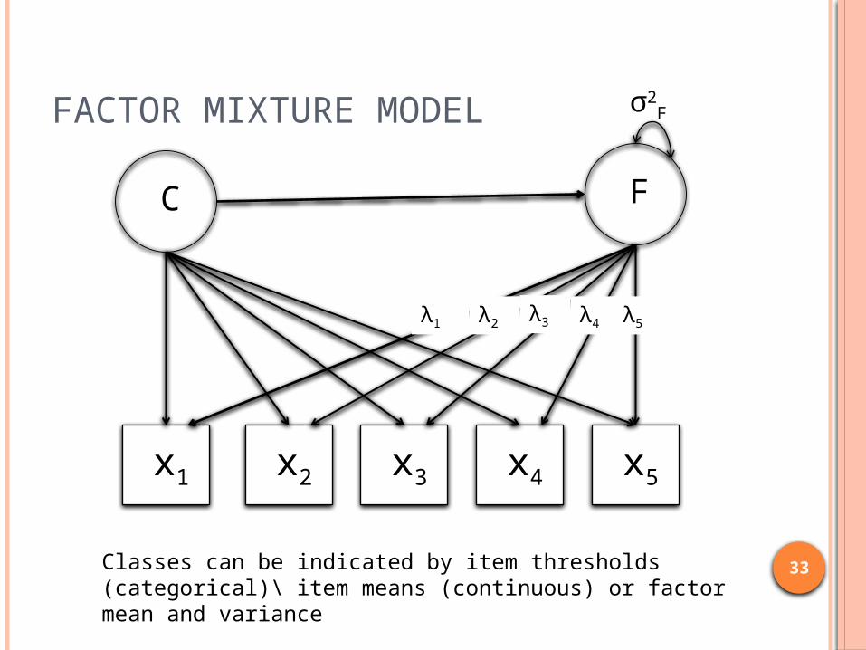
FACTOR MIXTURE MODEL σ2F

x1 x2 x3 x4 x5

C F

λ1 λ2 λ3 λ4 λ5

Classes can be indicated by item thresholds (categorical)\ item means (continuous) or factor mean and variance

34

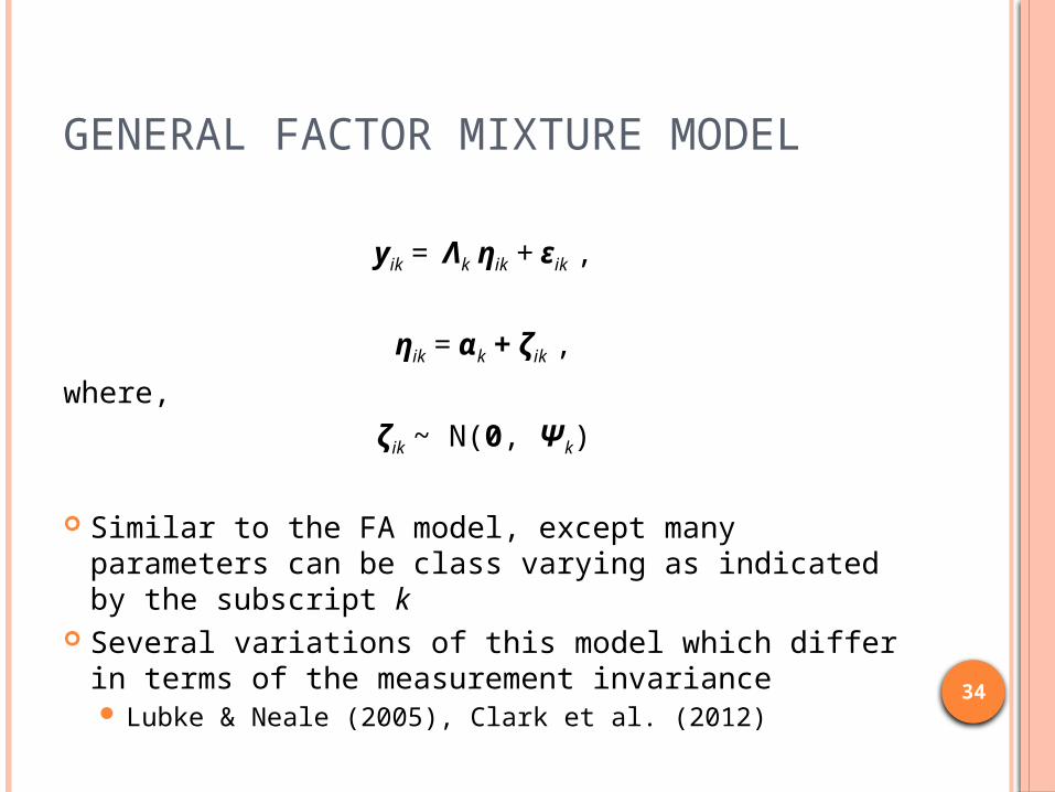
GENERAL FACTOR MIXTURE MODEL

yik = Λk ηik + εik ,

ηik = αk + ζik ,where,

ζik ~ N(0, Ψk)

Similar to the FA model, except many parameters can be class varying as indicated by the subscript k

Several variations of this model which differ in terms of the measurement invariance Lubke & Neale (2005), Clark et al. (2012)

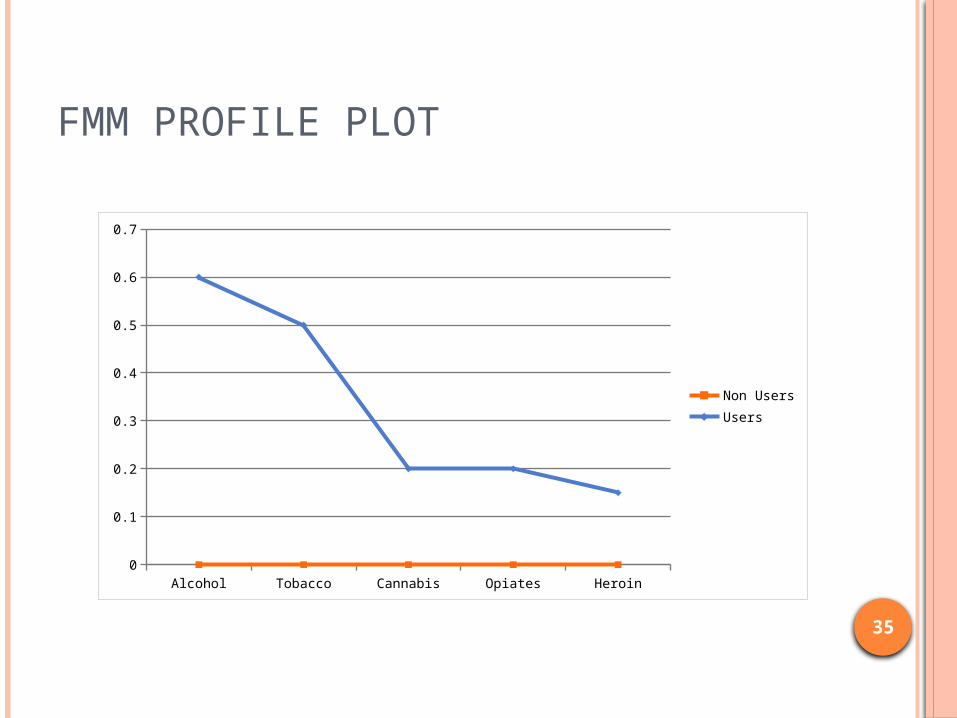
35

FMM PROFILE PLOT

Alcohol Tobacco Cannabis Opiates Heroin0

0.1

0.2

0.3

0.4

0.5

0.6

0.7

Non UsersUsers

36

HOW DO WE DO THIS IN OPENMX?

You’ll have to wait till tomorrow! Factor Mixture Model is a generalization of

the Growth Mixture Model we’ll talk about tomorrow afternoon.

37

MIXTURES & TWIN MODELSHow do we combine the ACDE model and mixtures?

38

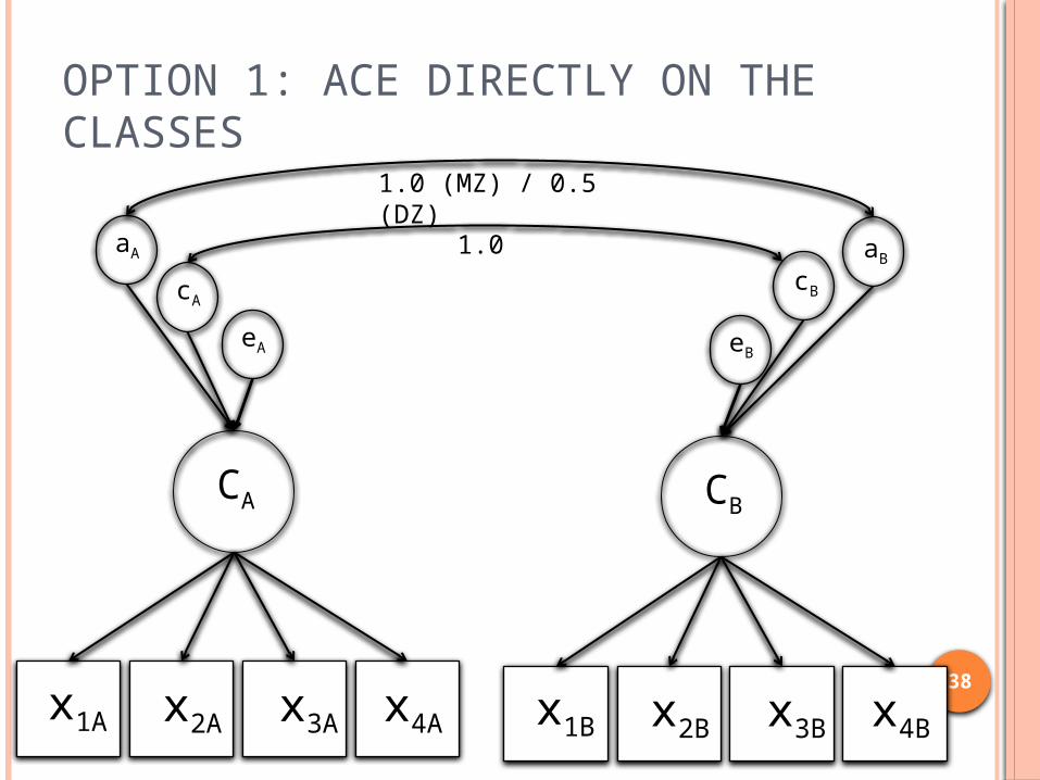
OPTION 1: ACE DIRECTLY ON THE CLASSES

x1A x2A x3A x4A

CA

aA

cA

eA

x1B x2B x3B x4B

CB

aBcB

eB

1.0

1.0 (MZ) / 0.5 (DZ)

39

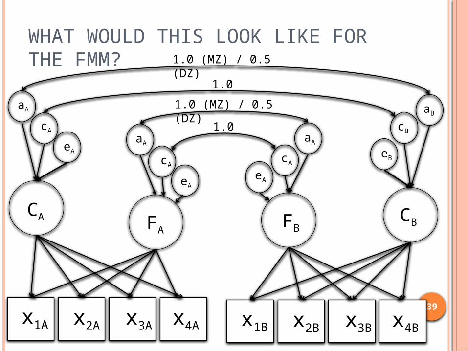
WHAT WOULD THIS LOOK LIKE FOR THE FMM?

x1A x2A x3A x4A

CA

aA

cA

eA

x1B x2B x3B x4B

CB

aB

cB

eB

1.0

1.0 (MZ) / 0.5 (DZ)

FA

eA

cA

aA

eA

cA

aA

1.0 (MZ) / 0.5 (DZ) 1.0

FB

40

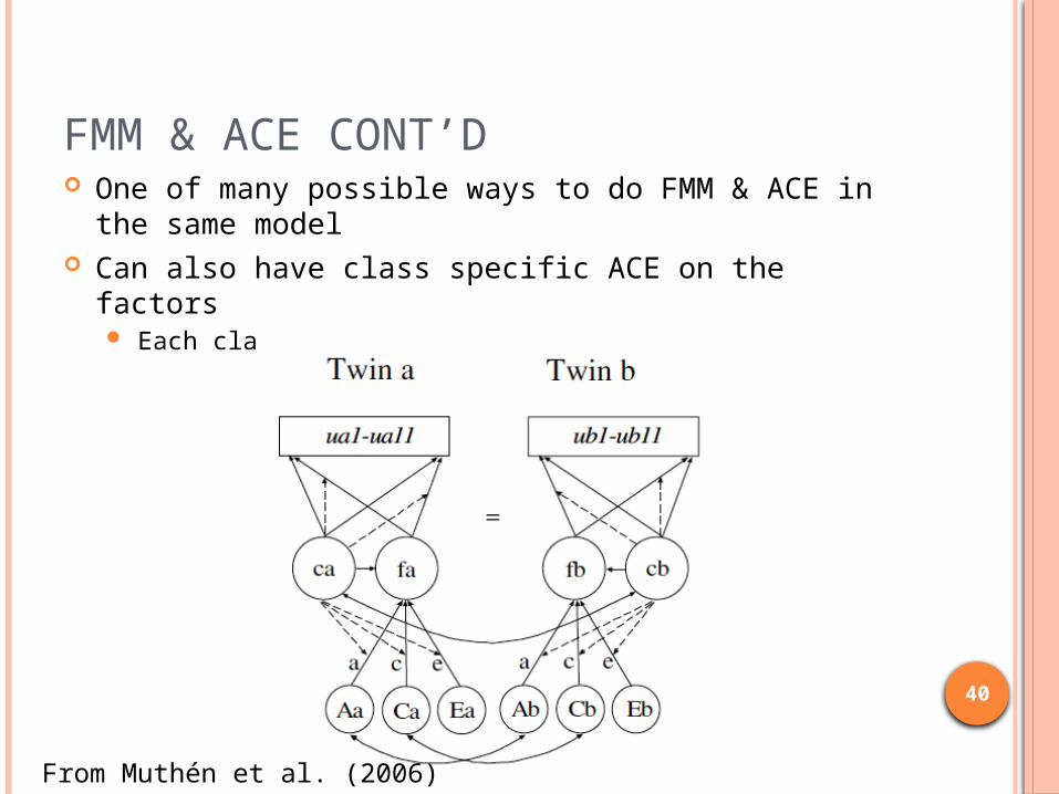
FMM & ACE CONT’D One of many possible ways to do FMM & ACE in the

same model Can also have class specific ACE on the factors

Each class has own heritability

From Muthén et al. (2006)

41

ISSUE WITH OPTION 1 Model is utilizes the liability threshold model

to “covert” the latent categorical variable, C, to a latent normal variable This requires that classes are ordered

Ex: high, medium, low users Don’t always have nicely ordered classes

Models are VERY time intensive Take a vacation for a week or two

42

OPTION 2: THREE-STEP METHOD1. Estimate mixture model2. Assign individuals into their most likely

latent class based on the posterior probabilities of class membership

3. Use the observed, categorical variable of assigned class membership as the phenotype in a liability threshold model version of ACE analysis

Note: Requires ordered classes

43

OPTION 2A Contingency table analysis using most likely

class membership Concordance between twins in terms of most likely

class membership If your classes are not ordered

Odds Ratio Excess twin concordance due to stronger genetic relationship

can be represented by the OR for MZ twins compared to the OR for DZ twins.

Place restrictions on the contingency table to test specific hypotheses Mendelian segregation, only shared environmental

effects Eaves (1993)

44

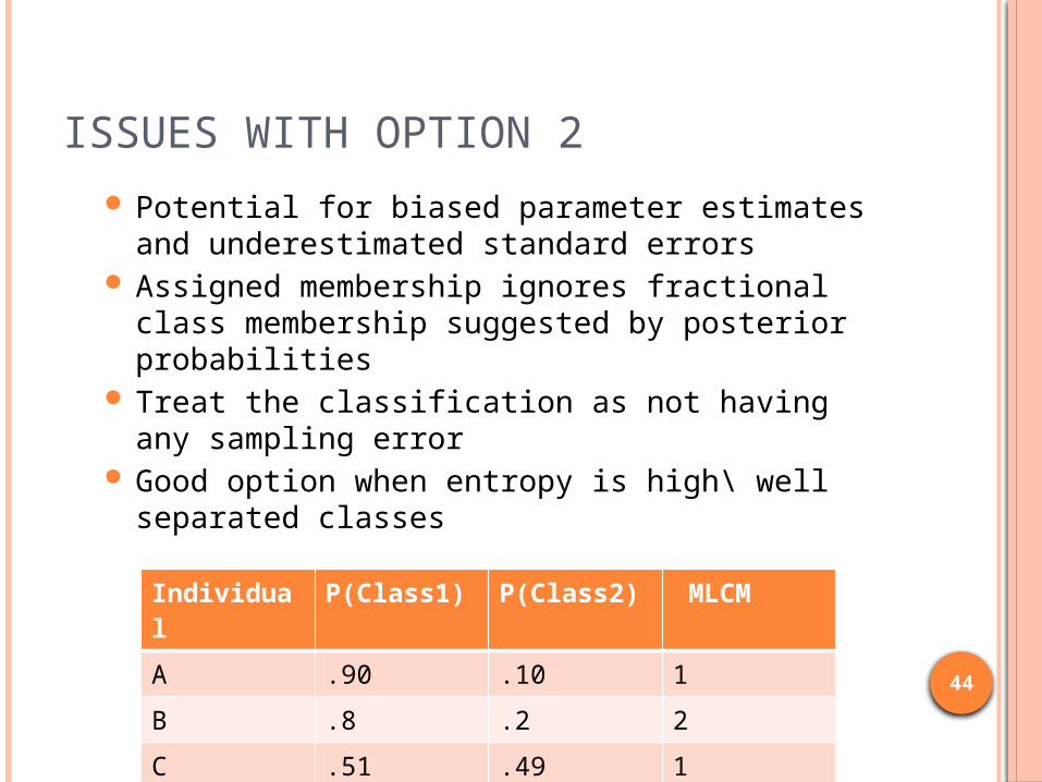
ISSUES WITH OPTION 2 Potential for biased parameter estimates and

underestimated standard errors Assigned membership ignores fractional class

membership suggested by posterior probabilities Treat the classification as not having any

sampling error Good option when entropy is high\ well

separated classes

Individual P(Class1) P(Class2) MLCMA .90 .10 1B .8 .2 2C .51 .49 1

45

SELECTION OF CROSS-SECTIONAL MIXTURE GENETIC ANALYSIS WRITINGS Latent Class Analysis

Eaves, 1993; Muthén et al., 2006; Clark, 2010

Factor Mixture Analysis Neale & Gillespie, 2005 (?); Clark, 2010; Clark et al.

(in preparation)

Additional References McLachlan, Do, & Ambroise, 2004

Mixtures in Substance Abuse Gillespie (2011, 2012)

Great cannabis examples