www.elsevier.com/locate/cis

Advances in Colloid and Interf

Brownian Dynamics, Molecular Dynamics, and Monte

Carlo modeling of colloidal systems

Jim C. Chena, Albert S. Kimb,*

aDepartment of Chemical Engineering, Environmental Engineering Program, Yale University, P.O. Box 208286, New Haven, CT 05620-8286, USAbDepartment of Civil and Environmental Engineering, University of Hawaii at Manoa, Honolulu, HI 96822, USA

Available online 13 November 2004

Abstract

This paper serves as an introductory review of Brownian Dynamics (BD), Molecular Dynamics (MD), and Monte Carlo (MC) modeling

techniques. These three simulation methods have proven to be exceptional investigative solutions for probing discrete molecular, ionic, and

colloidal motions at their basic microscopic levels. The review offers a general study of the classical theories and algorithms that are

foundational to Brownian Dynamics, Molecular Dynamics, and Monte Carlo simulations. Important topics of interest include fundamental

theories that govern Brownian motion, the Langevin equation, the Verlet algorithm, and the Metropolis method. Brownian Dynamics

demonstrates advantages over Molecular Dynamics as pertaining to the issue of time-scale separation. Monte Carlo methods exhibit strengths

in terms of ease of implementation. Hybrid techniques that combine these methods and draw from these efficacies are also presented. With

their rigorous microscopic approach, Brownian Dynamics, Molecular Dynamics, and Monte Carlo methods prove to be especially viable

modeling methods for problems with challenging complexities such as high-level particle concentration and multiple particle interactions.

These methods hold promising potential for effective modeling of transport in colloidal systems.

D 2004 Elsevier B.V. All rights reserved.

Keywords: Brownian Dynamics; Molecular Dynamics; Monte Carlo; Inter-particle interaction; Diffusivity; Stochastic force; Verlet algorithm; Langevin

equation; Metropolis method

Contents

1. Introduction. . . . . . . . . . . . . . . . . . . . . . . . . . . . . . . . . . . . . . . . . . . . . . . . . . . . . . . . . . . . 160

2. Background on Brownian motion . . . . . . . . . . . . . . . . . . . . . . . . . . . . . . . . . . . . . . . . . . . . . . . . 161

2.1. Defining the probability distributions for Brownian motion . . . . . . . . . . . . . . . . . . . . . . . . . . . . . . . 161

2.2. Quantification of the distribution P2 for discrete random walk . . . . . . . . . . . . . . . . . . . . . . . . . . . . . . 161

2.3. Modeling Brownian motion by a Gaussian probability distribution. . . . . . . . . . . . . . . . . . . . . . . . . . . . 162

2.4. Example of Brownian motion of a free particle. . . . . . . . . . . . . . . . . . . . . . . . . . . . . . . . . . . . . . 162

3. Brownian Dynamics . . . . . . . . . . . . . . . . . . . . . . . . . . . . . . . . . . . . . . . . . . . . . . . . . . . . . . . 162

3.1. Fundamental theory of Brownian Dynamics modeling . . . . . . . . . . . . . . . . . . . . . . . . . . . . . . . . . . 163

3.2. Incorporating inter-particle interactions . . . . . . . . . . . . . . . . . . . . . . . . . . . . . . . . . . . . . . . . . . 164

3.3. Numerical algorithms for Brownian Dynamics . . . . . . . . . . . . . . . . . . . . . . . . . . . . . . . . . . . . . . 165

3.4. Application to ionic solutions . . . . . . . . . . . . . . . . . . . . . . . . . . . . . . . . . . . . . . . . . . . . . . . 166

4. Molecular Dynamics . . . . . . . . . . . . . . . . . . . . . . . . . . . . . . . . . . . . . . . . . . . . . . . . . . . . . . . 166

4.1. Verlet algorithm . . . . . . . . . . . . . . . . . . . . . . . . . . . . . . . . . . . . . . . . . . . . . . . . . . . . . . 166

4.2. Critique of the Verlet algorithm . . . . . . . . . . . . . . . . . . . . . . . . . . . . . . . . . . . . . . . . . . . . . . 167

4.3. Implementing a modified pair potential . . . . . . . . . . . . . . . . . . . . . . . . . . . . . . . . . . . . . . . . . . 168

0001-8686/$ - see front matter D 2004 Elsevier B.V. All rights reserved.

doi:10.1016/j.cis.2004.10.001

* Corresponding author. Tel.: +1 808 956 3718; fax: +1 808 956 5014.

E-mail address: AlbertSK@hawaii.edu (A.S. Kim).

ace Science 112 (2004) 159–173

J.C. Chen, A.S. Kim / Advances in Colloid and Interface Science 112 (2004) 159–173160

4.4. Perturbation theory for MD. . . . . . . . . . . . . . . . . . . . . . . . . . . . . . . . . . . . . . . . . . . . . . . . 168

4.4.1. Theories of Kubo and Mori . . . . . . . . . . . . . . . . . . . . . . . . . . . . . . . . . . . . . . . . . . . 168

4.4.2. Application of perturbation theory for MD . . . . . . . . . . . . . . . . . . . . . . . . . . . . . . . . . . . 168

5. Combined BD–MD algorithm . . . . . . . . . . . . . . . . . . . . . . . . . . . . . . . . . . . . . . . . . . . . . . . . . . 169

6. Monte Carlo methods . . . . . . . . . . . . . . . . . . . . . . . . . . . . . . . . . . . . . . . . . . . . . . . . . . . . . . 170

6.1. Theory of Monte Carlo modeling. . . . . . . . . . . . . . . . . . . . . . . . . . . . . . . . . . . . . . . . . . . . . 170

6.2. Application of Monte Carlo methods to Brownian Dynamics . . . . . . . . . . . . . . . . . . . . . . . . . . . . . . 171

7. Concluding remarks . . . . . . . . . . . . . . . . . . . . . . . . . . . . . . . . . . . . . . . . . . . . . . . . . . . . . . . 172

Acknowledgement. . . . . . . . . . . . . . . . . . . . . . . . . . . . . . . . . . . . . . . . . . . . . . . . . . . . . . . . . . . 173

References. . . . . . . . . . . . . . . . . . . . . . . . . . . . . . . . . . . . . . . . . . . . . . . . . . . . . . . . . . . . . . . 173

1. Introduction

The purpose of this review paper is to introduce

Molecular Dynamics (MD), Brownian Dynamics (BD),

and Monte Carlo (MC) algorithms as alternatives for

modeling colloidal transport as opposed to more conven-

tional integral techniques such as the Ornstein-Zernike (OZ)

Integral Method with Hypernetted-Chain (HNC) or Percus-

Yevick (PY) closures. MD, BD, and MC algorithms offer

colloidal science the advantageous capability of rigorous

and meticulous accounting of discrete particle trajectories,

collisions, and configurations that constitute a precise

representation of the particle system at the microscopic

scale [1]. Furthermore, these models deconstruct the macro-

scopic system behavior into individual contributions from

the system’s foundational, underlying constituents. Such a

modeling approach strictly adheres to the actual system

composition as it definitively attributes system responses to

processes modeled to occur in its substructures. Therefore,

the modeled system behavior can be understood and

interpreted with precision and exactness. On the other hand,

continuum-level modeling such as the OZ Integral Method

describes the system using integrated average quantities of

system properties, such as the osmotic pressure, that provide

only a general representation. The macroscopic averaging of

system properties is susceptible to inaccuracy or divergence

when its approximations break down in the presence of

complicating factors such as strong inter-particle interac-

tions, high particle concentrations, and the onset of phase

transition of the suspension [2]. In practice, the HNC and

PY closures have been shown to be accurate up to a

maximum particle volume fractions of 0.3–0.4 beyond

which the models do not converge. Therefore, these

methods are incapable of modeling the phase transition of

particles that may occur at high volume fractions greater

than 0.5 [3].

Furthermore, situations with inter-particle interaction at

high particle volume fraction are better represented with

inclusion of multi-body contributions to a given model

which will again require approximations in the integral

techniques [4]. On the contrary, MD, BD, and MC are

capable of accounting for discrete multi-body contributions

with the computationally intensive summation of all

contributing particle interactions [5]. These modeling

techniques have been deployed to accurately model systems

of high particle volume fraction nearing the phase transition

limit under the influence of particle interactions [6]. There-

fore, the modeling methods are not only more fundamen-

tally precise in their depiction of the system but also more

robust when encountering complications and extreme

conditions. Incorporation of these modeling methods to

current modeling endeavors holds promising potential for

advancing the accuracy of numerical modeling and broad-

ening the range of applicability for theoretical understanding

of colloidal transport properties.

This study will review previous modeling efforts using

MD, BD, and MC as alternatives and improvements to

continuum-level modeling. Of particular interest, the review

will focus on algorithms for computing the thermodynamic

and transport coefficients under conditions with inter-

particle interaction. It will commence with a brief refresh-

ment of the fundamental theories for Brownian motion, a

critical element in the modeling of colloidal systems. The

stochastic nature of Brownian motion can only be approxi-

mated by macroscopic techniques and compels rigorous,

discrete accounting of individual particle trajectories to

achieve a true depiction of the process. From that back-

ground, the review will proceed to first address Brownian

Dynamics modeling. The fundamental theories of BD will

be discussed, followed by examples of its algorithms and

applications to ionic systems with inter-particle interactions.

Next, the Molecular Dynamics method will be reviewed

beginning with a discussion and critique of the Verlet

algorithm which is considered to be the classical technique

for MD modeling. The issue of modeling inter-particle

interactions will again be discussed. Review of one of the

more common usages of MD, perturbation theory, will

ensue. Subsequently, hybrid methods that combine both BD

and MD methods will be considered along with various

alternative techniques. The review will then transition into a

discussion of Monte Carlo techniques. Theories and variants

of MC will be presented, followed by examples of

applications of MC to model Brownian motion. Again,

various hybrid methods combining MC and MD will be

considered. The goal of this review is to bring about greater

awareness of the potential for breakthroughs in modeling of

J.C. Chen, A.S. Kim / Advances in Colloid and Interface Science 112 (2004) 159–173 161

colloidal transport encapsulated in MD, BD, and MC

methods. It is the aspiration of the authors that MD, BD,

and MC methods would undergo wider application in the

field of colloidal sciences.

2. Background on Brownian motion

2.1. Defining the probability distributions for Brownian

motion

To begin, a background on the fundamental theory of

Brownian motion is appropriate. An excellent resource on

the topic is the comprehensive review of Wang and

Uhlenbeck in 1945 [1] on Brownian motion for free

particles and the harmonic oscillator. In this work, Wang

and Uhlenbeck [1] methodically recount the statistical

properties of Brownian motion. As an introduction, trajec-

tories of particles undergoing Brownian motion can be

defined by a set of probability distributions where:

W1 yð Þdy ¼ probability of finding a particle in the range

y; yþ dyð Þ at time t:

W2 y1 y2tð Þdy1dy2 ¼ probability of finding a particle in the

range dy1 at time t1 and dy2 at a time t

¼ t2 � t1ð Þ apart: ð1Þ

and so on. More specifically, Brownian motion can be cast

as a Markoff process meaning that the position of a particle

at time tn is solely dependent upon its location at the

previous time tn�1. In the Markoff process, the particle

transitions from one location to the next by way of a

conditional probability P2( y1|y2,t)dy2 which signifies the

probability that given the particle location at y1, it will be

located in the range ( y2, y2+dy2) at a time t later. The

conditional probability P2 is related to the probability

distributions of Eq. (1) by:

W2 y1y2tð Þ ¼ W1 y1ð ÞP2 y1jy2tð Þ ð2Þ

So, from Eqs. (1) and (2) it is apparent that the quantitiesW2

and P2 essentially defines the entire process. Mapping

particle trajectory from Brownian motion becomes a task of

defining and sampling the probability distribution P2. A

necessary property of the distribution P2 is that it must obey

the condition:

P2 y1jy2; tð Þ ¼Z

dyVP2 y1jyV; t0ð ÞP2 yVjy2; t � t0ð Þ ð3Þ

where t0= tV�t1 and t1b tVb t2.This is the well-known Smoluchowski Equation [7]

which is the basis for the theory of Brownian motion. Thus,

the derivation of the probability distribution that governs the

Markovian process of Brownian motion is validated by its

agreement with the normative Smoluchowski Equation.

What remains now is to explicitly quantify the function P2.

A simple introductory example will be given in Section 2.2

to serve as the foundation for the subsequent more realistic

models.

2.2. Quantification of the distribution P2 for discrete

random walk

So, it has been shown that for a Markoff process such as

Brownian Motion, the system behavior is completely

governed by the conditional probability P2. A simple

example involving a discrete random walk scenario will

bring forth the application of the theory. In a one-dimen-

sional discrete random walk, a particle traverses on a

straight line making steps of size D forwards or backwards

with equal probability at each time t. In this case, the

conditional probability P(n|m,s) that a particle positioned at

nD at t=0 will be located at mD at time t=ss (s=time

interval, s=1, 2, 3, . . .) will be:

P njm; sð Þ ¼ s!

vþ s

2

� �!v� s

2

� �!

1

2

� �s

ð4Þ

where v=|m�n|. Eq. (2) is thus readily computable and can

be implemented in algorithms that model the stochastic

nature of one-dimensional random walk by sampling this

probability distribution.

In a more interesting scenario, this initial physical model

can be advanced with the addition of the Ehrenfest transition

probability [8] where the particle moves not with equal

probability forward and backward but instead are more

attracted to designated points. For instance, in the situation

where a particle is attracted to initial point n, the transition

probability distribution becomes:

Q njm; sð Þ ¼ Rþ n

2Rd m; n� 1ð Þ þ R� n

2Rd m; nþ 1ð Þ ð5Þ

where d is the Kronecker delta and R is a given integer

characteristic of the particular system. The particle now does

not travel with equal probability forward and backward but

instead with probabilities 12

1� nR

� �and 1

21þ n

R

� �; respec-

tively. The particle will then exhibit a tendency to move

towards the point n. This extension mimics the influence of

inter-particle interaction which is a frequent complication in

colloidal transport problems. Eqs. (4) and (5) therefore offer

fundamental models of one-dimensional random walk. This

basic model can be applied to more complex problems

involving two- and three-dimensional motion by sampling

these probability distributions for particle motion in each

coordinate direction. Details of this derivation are given in

Wang and Uhlenbeck in 1945 [1]. Thorough discussions on

random walk particle motion can be found in the classical

J.C. Chen, A.S. Kim / Advances in Colloid and Interface Science 112 (2004) 159–173162

paper by Chandrasekhar [9]. The mathematical formulation

and physical depiction described above constitute the basic

theory for the rigorous modeling of Brownian motion to

follow.

2.3. Modeling Brownian motion by a Gaussian probability

distribution

The Gaussian random process typifies the stochastic

nature of many natural phenomena including Brownian

motion. Wang and Uhlenbeck in 1945 [1] prove that for a

Gaussian random process, the spectral density of the

probability distribution represents the governing parameter

of the system behavior. So, the Gaussian random probability

distribution of the particle position y(t) over a long time T

should be written as a Fourier series of the form:

y tð Þ ¼Xlk¼1

akcos2pk

Tt þ bksin2p

k

Tt

� �ð6Þ

where ak and bk are independent random variables with

Gaussian distribution. It should be noted that the summation

begins at k=1 because hyi=0.Wang and Uhlenbeck show that

astute utilization of mathematical theorems of Gaussian

distributions and applying them to the formulated Fourier

series will readily generate the various types of probability

functions that define Brownian motion. For instance, the

mean square value of the particle velocity at a given time t

will be:

hyy tð Þ2iAv ¼ 4p2

Z l

0

f 2G fð Þdf ð7Þ

where f=k/T and G is the spectral density of the Gaussian

random variable y(t). It becomes apparent here that the

spectral density G is indeed the defining quantity of the

Gaussian process. The spectral density can be obtained from

the Langevin Equation of the particle motion as will be shown

in Section 2.4.

2.4. Example of Brownian motion of a free particle

Wang and Uhlenbeck in 1945 [1] proceed to present the

application of the above theory to the example of the

Brownian motion of a free particle. The governing equation

of motion is the well-known Langevin Equation with its

general form given as:

dyy

dtþ byy ¼ F tð Þ ð8Þ

where b is the friction coefficient and F(t) is a random

fluctuating force of the system. If 4D is taken as the spectral

density of the random force F(t), then in turn, the spectral

density, Gy( f), of the Gaussian random variable y(t)

becomes:

Gy fð Þ ¼ 4D

b2 þ 2pfð Þ2ð9Þ

From that the two-dimensional Gaussian distribution of the

particle position follows as:

W2 y1y2tð Þ ¼ b

2pD 1� q2ð Þ1=2

exp � b2D 1� q2ð Þ y21 þ y22 � 2qy1y2

� �ð10Þ

where q=hy1y2iAv/hy12iAvhy22iAv is the correlation

coefficient.

The distribution W2 is sufficient to map the particle

trajectory. Eq. (10) can be implemented into algorithms that

seek to model Brownian motion. Again, extension to two-

and three-dimensional motion can be attained by applying

this procedure to each direction of motion.

3. Brownian Dynamics

Having re-developed the theoretical foundation of Brownian motion, the review proper will embark first on a discourse on

Brownian Dynamics with its fundamental theory, algorithms, and applications. The uniqueness of BD lies in its capability to

account for timescale separation, a complication problematic to MD modeling. Timescale separation depicts situations where

one type of motion in the system occurs at much more rapid times than the others. Timescale separation compels MD modeling

to take small time steps in order to synchronize with the rapid variations. In systems where the rapid process is not of interest,

timescale separation introduces an irrelevant complication that slows the modeling procedure. So, BD offers an efficient

alternative that bypasses this hindrance by considering the stochastic properties of the rapidly varying quantities in the system.

Sampling the probability distributions of the stochastic processes does compromise a strict microscopic view of the system.

However, discrete accounting of individual particle motion is still maintained, and so BD remains classifiable as a rigorous

microscopic modeling technique. The essential theories, applications, and continuing developments of BD will be surveyed

here.

J.C. Chen, A.S. Kim / Advances in Colloid and Interface Science 112 (2004) 159–173 163

3.1. Fundamental theory of Brownian Dynamics modeling

Overviews of the fundamental theories of Brownian Dynamics are given in Ermak [2], Ermak and Buckholtz [3], and Van

Gunsteren and Berendsen [4]. The governing equation for BD is the Langevin Equation given here with consideration for

particle interactions:

mvv tð Þ ¼ � cmv tð Þ þ f tð Þ þ R tð Þ ð11Þ

where m is the particle mass. Here, c represents the friction coefficient that produces a non-conservative, non-systematic force

induced by the solvent (e.g. frictional forces) and f(t) adds a conservative, systematic force due to the inter-particle potential.

Of particular interest here is the characteristics of the conserved random force R(t) that is responsible for the Brownian motion.

Referring to the discussion in Section 2, the Brownian motion is taken to be a random Gaussian process with properties given

by Eq. (10). Various methods are available for integration of Eq. (11) to obtain an algorithm for the particle displacement. One

possibility is given by Van Gunsteren and Berendsen in 1982 [4] for a one-component atomic system. The algorithms for

particle displacement in their work are:

r tn þ Dtð Þ ¼ r tnð Þ 1þ exp � cDtð Þ½ � � r tn � Dtð Þexp � cDtð Þ þ f tnð Þ Dtð Þ2 1� exp � cDtð Þ½ �mcDt

þff tnð Þ Dtð Þ3 1

2cDt 1þ exp � cDtð Þ½ � � 1� exp � cDtð Þ½ �

m cDtð Þ2

þ Xn Dtð Þ þ exp � cDtð ÞXn � Dtð Þ þ O Dtð Þ4h i

v tnð Þ ¼r tn þ Dtð Þ � r tn � Dtð Þ½ � þ f tnð Þ Dtð Þ2G cDtð Þ

m cDtð Þ2� ff tnð Þ Dtð Þ3G cDtð Þ

m cDtð Þ3þ Xn � Dtð Þ � Xn Dtð Þ½ �

( )H cDtð Þ

Dtð12Þ

where f(tn) is the systematic force derived from the inter-particle interaction and:

Xn Dtð Þ ¼

Z tnþDt

tn

1� exp � c tn þ Dt � tð Þ½ �f gR tð Þdt

mc

G cDtð Þ ¼ exp cDtð Þ � 2cDt � exp � cDtð Þ

H cDtð Þ ¼ cDtexp cDtð Þ � exp � cDtð Þ½ � ð13Þ

with Xn(Dt) being a random variable that characterizes the random force R(t). The random force, R(t), exhibits the statistical

properties:

hRi 0ð ÞRj tð Þi ¼ 2micikBTdi;jd tð Þ

W Rið Þ ¼ 2phR2i i

� ��1=2exp � R2

i =2hR2i i

hRii ¼ 0

hvi 0ð ÞRj tð Þi ¼ 0; tz0

hfi 0ð ÞRj tð Þ ¼ 0; tz0 ð14Þ

where h. . .i denotes the average over an ensemble, subscripts i and j classify the components of the ensemble, kB is the

Boltzmann’s constant, T is the reference temperature, di,j is the Kronecker delta, and W(Ri) denotes the Gaussian distribution

of the random force R(t). The solution procedure then becomes a matter of integrating the random force, inputting

J.C. Chen, A.S. Kim / Advances in Colloid and Interface Science 112 (2004) 159–173164

l

.

,

the systematic and non-systematic forces, and mapping the particle trajectories according to Eq. (12). Details of the algorithm

are given in Sections 3.2–3.4.

3.2. Incorporating inter-particle interactions

When applying BD modeling to colloidal systems in solution, a critical issue to consider is the role of inter-particle

interactions that produce the systematic force as described by Eq. (11). The influence of inter-particle interactions becomes

especially important when the system approaches high-particle concentrations nearing the phase transition limit where

appreciable portions of the inter-particle potential arise from many-body contributions. In fact, Verlet in 1967 [5], in his

classical work on MD modeling, remarks that the choice of the model for inter-particle interactions is among the most crucial

determining factors of the accuracy and range of capability of the model. Therefore, any modeling endeavor of particle systems

in liquid must place proper emphasis on representative evaluation of the inter-particle interactions occurring throughout the

range of experimental conditions.

Allen in 1980 [6] presents a Brownian Dynamics model for simulating chemical reactions in a particle system in solution

that includes three types of interparticle-interaction terms. In this study, Allen considers the situation where a particle B is

transferred between two substrates A and C:

A� B: : :C V A: : :B� C ð15Þ

where the dash (–) signifies a bond between two particles and the dotted line (d d d ) signifies that the two particles are

detached. This scenario should be expected in highly concentrated particle suspensions and mimics the process of particle

detachment and coagulation. The significance of three-body interactions is clearly evident. Allen [6] considers three

contributions to the inter-particle interaction, the Lennard–Jones potential between particle pairs, the attraction between

bonded pairs in the chemical reaction, and a three-body potential that facilitates the chemical reaction. Of interest here is

the Lennard–Jones potential which is a commonly employed model for computing the pairwise inter-particle potentia

given as:

VLJ r1;2� �

¼ 4eLJrr1;2

� �12

� rr1;2

� �6" #

ð16Þ

where r1,2 is the inter-particle separation, r is the radius of the particle, and ELJ the characteristic potential energy

minimum of the interaction between the two particles. The Lennard–Jones potential may be adequate for dilute systems

where particle B experiences predominately the potential from particle A. However, in cases where particle C lies in close

proximity to the pair A–B, the strictly pairwise potential of Eq. (16) should be modified to account for the third particle

Allen [6] suggests that the modeling of the inter-particle potential can be improved by replacing the Lennard–Jones

potential of Eq. (16) with an improved form given in Allen [6] that utilizes the pair-distribution function g(r1,2) in the

Lennard–Jones liquid at the chosen temperature and density:

V g r1;2� �

¼ � kBT lng r1;2� �

ð17Þ

The pair-distribution function may be computed from the discrete particle locations in the suspension. Incorporating the

pair-distribution function will provide additional consideration for the multi-body correlations, whether pair-wise or greater

that the potential will induce within the particle system. This approach to computing the pair-distribution function improves the

inaccuracies of the pair-distribution function at high concentrations (upper limit of approximately volume fraction 0.4 [10])

when deriving it from the inter-particle potential [11]. A further improvement would be to employ a three-body potential for a

colloidal triplet in an equilateral triangular configuration as given in Wu et al. [10] by first considering the contribution of

three-body effects to the inter-particle force:

DF3 ¼2F3

3� F2 ð18Þ

where DF3 is the additional three-body contribution to the inter-particle force, F3 is the average total force between two

particles in a three-body system, and F2 is the force between two isolated particles without three-body effects. The three-body

potential follows from the integration of the force. Of course, it should be noted here that Eq. (18) is valid specifically for an

equilateral triangular such as when the colloidal suspension approaches a face-centered-cubic or body-centered-cubic ordered

structure. So, the three-body potential derived by Wu et al. [10] may become useful in situations where the suspension

approaches solidification to an ordered structure. In a modeling algorithm, Eq. (18) can be applied at each time step to compute

the adjustments needed to the pair-wise potential from three-body effects.

J.C. Chen, A.S. Kim / Advances in Colloid and Interface Science 112 (2004) 159–173 165

Such an approach discretely accounts for individual particle contributions and so would not be hindered by limits of particle

concentration. The detraction of a three-body potential stems from the exponential rise in the computation time that renders

many such models highly impractical. Turq et al. in 1979 [11] offer a less computationally intensive method for including

many-body interactions using the Ewald method. The resulting inter-particle potential is given as:

V1;2 r1;2� �

¼ e2

nca14þ a24ð Þ

� �a14þ a24ð Þr1;2

� �nc

� e1e2

er1;2ð19Þ

where a1* and a2* are the Pauling ionic radii of the particle pair, e1 and e2 are the particle charges, E is the dielectric constant of

the medium, and nc is a parameter of the system. Eq. (19) includes the influence of neighboring particles to each pairwise

potential. Details of this method are given in Lewis and Singer in 1975 [12].

For a particle system in liquid, the proper choice for modeling the inter-particle interaction should be regarded as a key step

in the theoretical development. In particular, for systems of high particle concentration, usage of purely pairwise potentials

such as the Lennard–Jones potential should be undertaken with caution, and considerations for many-body contributions are

desirable. Duly noted is that the demands for computational efficiency may dictate relaxation of a strict adherence to modeling

a many-body system.

3.3. Numerical algorithms for Brownian Dynamics

Given the fundamental theories for depicting stochastic Brownian motion and inter-particle interactions presented in

Sections 3.1 and 3.2, an executable numerical algorithm for mapping particle trajectories can be devised. Van Gunsteren and

Berendsen in 1982 [4] present a BD algorithm that proves to be more robust than previous algorithms by allowing for a varying

Fig. 1. Flow chart for a typical BD algorithm from Van Gunsteren and Berendsen [4].

Table 1

Experimental conditions for modeling in Turq et al. [13]

Parameters Cation Anion

Number of particles 32 32

Mass (atomic units) 23 35.5

Charge 1 �1

D (105 cm2/s) 1.335 2.035

tp (momentum correlation time in ps) 0.01239 0.02914

Aqueous solution with 1 M NaCl at 25 8C. D is the Stokes–Einstein

diffusivity.

J.C. Chen, A.S. Kim / Advances in Colloid and Interface Science 112 (2004) 159–173166

,

l

.

random force within each time step and is based on the well-known Verlet MD algorithm. The modeling procedure initiates

with the ordinary Langevin equation which is integrated to produce expressions for particle displacement and velocity similar

to that given in Eq. (12). The solution procedure is given in Fig. 1. Details of the theoretical development and numerical

algorithm are given in Van Gunsteren and Berendsen [4].

Key attributes of the algorithm of Van Gunsteren and Berenden [4] are first that it conforms to the classical Verlet algorithm

in the limit of zero friction (c=0). This convergence accords the algorithm with validation in agreement with a generally

accepted and established algorithm. Secondly, the derivation of Van Gunsteren and Berenden [4] does not assume the random

force to be constant within each time step of the algorithm which is the assumption used in Turq et al. [13]. Rather, the random

force is integrated with consideration for its statistical properties in the form of probability distributions. The assumption of a

constant random force at each time step requires that the time step be much smaller than the velocity relaxation time (DtVc�1).

Such a restriction results in much longer computation times due to the small step size. The algorithm of Van Gunsteren and

Berenden [4] circumvents that restriction and delivers a faster computation scheme.

3.4. Application to ionic solutions

Having derived algorithms for BD, direct practical application to physical systems can now be examined. Turq et al. in

1977 [13] utilize BD to model the motion of interacting ions in an electrolyte solution. Their formulation aligns with the

discussions given in Sections 3.1–3.3. The inter-particle potential given in Eq. (19) is selected in their model. The experimental

conditions for their simulation are given in Table 1. Using their algorithm for BD such as described in Section 3.3, the

trajectory of the collection of particle motion in the system is mapped. From that, the diffusivity of the system can be computed

according to:

D ¼ limtYl

hr tð Þ2i6t

ð20Þ

Results of their model show that the diffusivities for the cation and anion computed from BD (D+=1.15105 and

D�=1.55105 cm2/s) agree with experimental measurements (D+=1.225105 and D�=1.795105 cm2/s). The effects of the

inter-particle potential causes computed diffusivities to differ appreciably from the Stokes–Einstein diffusivities given in Table

1. So, an application of BD to successfully model particle motion in ionic solution is offered by Turq et al. [13]. Worthy of note

is that the modeling is undertaken for ionic systems with electrolyte molarity of 1 M. These experimental conditions are not

representative of highly concentrated particle suspensions nearing the phase transition. Furthermore, the model of the method

of Turq et al. [13] is susceptible to the critique raised in Section 3.3 for their assumption of a constant random force at each

time step. In fact, the restriction on the size of the time step is only loosely met in their study. The work of Turq et al. [13] offer

a useful application of BD to the computation of thermodynamic and transport coefficients, but further developments to their

theoretical formulation and testing of their results can still improve their model.

4. Molecular Dynamics

Molecular Dynamics takes the exhaustive approach of

discrete accounting of forces exerted on each particle of

the system without the approximations inherent in sam-

pling of probability distributions as in BD. The modeling

procedure casts the particle system as a system of

Newtonian mechanics equations of motion. Forces that

would be encountered in systems of interest to this study

would include inter-particle interactions, diffusive forces

osmotic pressure, and external forces. Once the canonica

equations are specified, the solution procedure becomes a

matter of solving the system of N partial differential

equations. The numerical method of choice has been finite

difference of time.

4.1. Verlet algorithm

The generally accepted classical algorithm for MD has

been the Verlet algorithm. Verlet [5] provides exposition of

his technique and categorizes it to be an bexactQ method

The modeling procedure begins by casting the system in

terms of its Newtonian equation of motion of each

individual particle of the system:

md2 ri

Y

dt2¼Xip j

FY

ri;j� �

ð21Þ

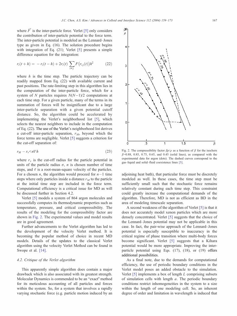
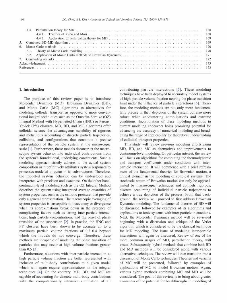
Fig. 2. The compressibility factor bp/q as a function of b for the isochors

b=0.88, 0.85, 0.75, 0.65, and 0.45 (solid lines), as compared with the

experimental data for argon (dots). The dashed curves correspond to the

gas–liquid and solid–fluid coexistence lines [5].

J.C. Chen, A.S. Kim / Advances in Colloid and Interface Science 112 (2004) 159–173 167

where FY

is the inter-particle force. Verlet [5] only considers

the contribution of inter-particle potential to the force term.

The inter-particle potential is modeled as the Lennard–Jones

type as given in Eq. (16). The solution procedure begins

with integration of Eq. (21). Verlet [5] presents a simple

difference equation for the integration:

ri t þ hð Þ ¼ � ri t � hð Þ þ 2ri tð ÞXip j

F ri;j tð Þ� �

h2 ð22Þ

where h is the time step. The particle trajectory can be

readily mapped from Eq. (22) with available current and

past positions. The rate-limiting step in this algorithm lies in

the computation of the inter-particle force, which for a

system of N particles requires N(N�1)/2 computations at

each time step. For a given particle, many of the terms in its

summation of forces will be insignificant due to a large

inter-particle separation with a given potential cutoff

distance. So, the algorithm could be accelerated by

implementing the Verlet’s neighborhood list [5], which

selects the nearest neighbors to include in the computation

of Eq. (22). The use of the VerletTs neighborhood list derivesa cut-off inter-particle separation, rM, beyond which the

force terms are negligible. Verlet [5] suggests a criterion for

the cut-off separation of:

rM � rvbnvPh ð23Þ

where rv is the cut-off radius for the particle potential in

units of the particle radius r, n is chosen number of time

steps, and v is a root-mean-square velocity of the particles.

For a chosen n, the algorithm would proceed for n�1 time

steps where only particles inside a distance rM to the particle

at the initial time step are included in the force term.

Computational efficiency is a critical issue for MD as will

be discussed further in Section 4.2.

Verlet [5] models a system of 864 argon molecules and

successfully computes its thermodynamic properties such as

temperature, pressure, and critical compressibility. The

results of the modeling for the compressibility factor are

shown in Fig. 2. The experimental values and model results

are in good agreement.

Further advancements to the Verlet algorithm has led to

the development of the velocity Verlet method. It is

becoming the popular method of choice in recent MD

models. Details of the updates to the classical Verlet

algorithm using the velocity Verlet Method can be found in

Swope et al. [14].

4.2. Critique of the Verlet algorithm

This apparently simple algorithm does contain a major

drawback which is also associated with its greatest strength.

Molecular Dynamics is commended to be an bexactQ method

for its meticulous accounting of all particles and forces

within the system. So, for a system that involves a rapidly

varying stochastic force (e.g. particle motion induced by an

adjoining heat bath), that particular force must be discretely

modeled as well. In these cases, the time step must be

sufficiently small such that the stochastic force remains

relatively constant during each time step. This constraint

could greatly increase the computational demands of the

algorithm. Therefore, MD is not as efficient as BD in the

area of modeling timescale separation.

A second weakness of the algorithm of Verlet [5] is that it

does not accurately model xenon particles which are more

densely concentrated. Verlet [5] suggests that the choice of

the Lennard–Jones potential may not be applicable in this

case. In fact, the pair-wise approach of the Lennard–Jones

potential is especially susceptible to inaccuracy in the

critical regime of phase transition where multi-body forces

become significant. Verlet [5] suggests that a Kihara

potential would be more appropriate. Improving the inter-

particle potential using Eqs. (17), (18), or (19) offers

additional possibilities.

As a final note, due to the demands for computational

efficiency, the use of periodic boundary conditions in the

Verlet model poses an added obstacle to the simulation.

Verlet [5] implements a box of length L comprising subsets

of simulation cells with length a. The periodic boundary

conditions restrict inhomogeneities in the system to a size

within the length of one modeling cell. So, an inherent

degree of order and limitation in wavelength is induced that

J.C. Chen, A.S. Kim / Advances in Colloid and Interface Science 112 (2004) 159–173168

represses the possibility of two-phase coexistence. In

general, the restriction due to the periodic boundary

condition is unavoidable. However, it can be controlled by

proper selection of the number of particles per simulation

cell and cell size.

4.3. Implementing a modified pair potential

Ermak [2] presents a modified pair potential as a more

complete model of inter-particle interaction over the

Lennard–Jones potential to model the motion of charged

particles in ionic solution. The derivation begins with

Poisson’s equation and accounts for contributions from

each particle in the system:

j2V rð Þ ¼ � 4pe

� �q rð Þ ð24Þ

where q(r) is the charge distribution of particles and ions in

the solution and E is the dielectric constant of the medium.

The charge distribution at each location r includes one

particle of charge �Nq, N+M counterions of charge +q, and

M by-ions of charge �q. Each such system constitutes a

basic modeling box of length L. This charge distribution at a

given basic modeling box can be written as a Fourier series:

q rð Þ ¼XNt

i¼1

aiXNt

k¼1

eik r�rið Þ

ai ¼þ 1 for 1V iVN þM

� 1 for N þM þ 1V iVN þ 2M

� N for i ¼ N þ 2M þ 1 ¼ Nt

8<: ð25Þ

The potential distribution in each basic modeling box can be

written in periodic form as:

V rð Þ ¼ 4pqevcell

XNt

i¼1

aiXNt

k¼1

1

k2eik r�rið Þ ð26Þ

where vcell is the volume of the basic modeling box. The

overall potential of one basic box is then:

U ¼ 1

2

Zvcell

q rð ÞV rð Þdvcell �q2

2e

XNt

i¼1

a2i

Zvcell

d r � rið Þjr � rij

dvcell

ð27Þ

From Eq. (27), the inter-particle force is simply the gradient

of the potentials. The advantage of this technique is that it

reduces the number of terms in the summation of inter-

particle interactions to those inside the basic box but still

includes contributions from outside the box by computing

the gradients of the overall potential U. The result is a great

reduction in the computational demand. This strategy can be

adapted to highly concentrated particle systems by grouping

the particles into basic boxes such that overall potentials U

in each cell can be used to compute the inter-particle

potentials with a given particle i. The traditional method of

Ermark given in Eqs. (24)–(27) has been updated recently

by such techniques as the mesh Ewald [15,16] and the fast

multiple method of Greengard [17].

4.4. Perturbation theory for MD

4.4.1. Theories of Kubo and Mori

An often-employed method of MD is perturbation theory.

Perturbation theory computes transport coefficients, such as

the diffusivity, as a linear response of an external field. In

these situations, the external field does not induce a phase

transition of the particles. Kubo [18] extensively develops

the principles that govern perturbation theory and its

applicability to the computation of dynamical constants

such as the diffusivity. The method entails subjecting the

system to a perturbing force and quantifying the system

response in terms of time correlations between the perturbed

and unperturbed systems. Using this idea, Kubo [18] derives

the fundamental relation that the diffusivity can be

computed from the time correlations of the velocities of

particles in the system. The derivation of the theory is too

involved to be presented here and so the reader is referred to

Kubo [18] for details of the theoretical formulation.

The Kubo theory does impose a restriction in that it is

only applicable to perturbations that are external to the

system. Situations where the concentration gradient induces

a perturbation in the form of a diffusive flux cannot be

modeled by this theory. But Kubo’s theory is useful for

modeling interparticle interactions as the perturbation. The

case of internal perturbations for a dilute system is treated

by Mori [19]. Here, the diffusion caused by internal

perturbations such as concentration gradients is computed

from the conjugate fluxes of state variables. Again due to

the lengthy derivation, the reader is referred to details given

in Mori [19].

The theoretical developments of Kubo [18] and Mori

[19] form the fundamental principles for MD modeling by

perturbation theory. An example of the application of this

modeling approach will be discussed in Sections 4.4.2

and 5.

4.4.2. Application of perturbation theory for MD

Ciccotti et al. [20] present a perturbation method for MD

to compute the transport coefficients based upon the theory

of Kubo [18]. The premise is that if during each step of an

MD algorithm a perturbation is applied to the system (e.g.

adjustments to particle coordinates or momentum), the time

correlation between the system behaviors of the perturbed

and unperturbed systems will yield the transport coeffi-

cients. For example, if a(r) is a dynamical variable of

interest distributed throughout a system of N particles, then

Kubo’s theory yields:

a rð Þ ¼XNi¼1

aid r � rið Þ ð28Þ

J.C. Chen, A.S. Kim / Advances in Colloid and Interface Science 112 (2004) 159–173 169

Suppose the system is perturbed at time t=0 by an external

field /(r,t). The Hamiltonian of the perturbed system would

be:

H ¼ H0 þ H1 tð Þ ð29Þ

where H0 and H1(t) are the Hamiltonians of the unperturbed

system and the perturbation, respectively. The mean change

in an observable property O of the system at time t=s can be

expressed in terms an autocorrelation function in Fourier

space:

hOO kð Þis ¼ bVZ s

�ldtVhOO k; sð ÞJJ a � k; tVð Þi0ik/ k; tVð Þ

ð30Þ

where b=1/kBT, V is the volume of the system, and Ja is the

current corresponding to the dynamical variable a that in

Cartesian coordinates satisfies:

aa r; tð Þ þjJ a r; tð Þ ¼ 0 ð31Þ

The general derivation given above can be clarified by a

specific application. Ciccotti et al. [20] uses perturbation

theory to compute the thermal conductivity k of a particle

system by introducing an energy fluctuation as the

perturbation. The result for the system response is:

kT ¼ bVZ l

0

dtVhJJ ex 0; tVð ÞJJ e

x 0; 0ð Þi0 ð32Þ

where Jxe is the energy current in the x direction and satisfies

the conservation given in Eq. (31) for the energy of the

system. This application for computing the thermal con-

ductivity can be readily translated to the case for calculating

the transport diffusivity. Eq. (31) can be converted to an

expression for mass transport by replacing the current J by

mass flux of particles and the dynamical variable a by the

particle mass. Eq. (32) would then become an expression for

the diffusivity in terms of the autocorrelation of the mass

fluxes.

The algorithm for perturbation theory would perform a

typical MD simulation as given in Section 4.4.1. At each

time step, the perturbation is introduced and the correspond-

ing fluxes computed (e.g. the particle mass fluxes are

computed from the particle trajectories mapped by MD).

Next, the responses are computed according to Eq. (32) to

yield the transport coefficients of interest at that time step.

So, perturbation theory presents an alternative for comput-

ing thermodynamic coefficients using MD. It should be

noted once again that the diffusivity computed here is the

mutual diffusion coefficient of binary mixtures or the self-

diffusion coefficient of a one component suspension.

Perturbations arising from an internal concentration gradient

cannot be accommodated by this method. Mori [19]

addresses the issue of concentration gradient driven

diffusion in a dilute system.

5. Combined BD–MD algorithm

As mentioned in Section 3, an important strength of the

BD method lies in its capability of coping with high-

frequency stochastic forces that confound MD methods. On

the other hand, MD boasts of strengths in its comprehensive

accounting of forces and simplicity of implementation as

shown in Section 4. A combination of the two methods

could reap the benefits of each. Ciccotti et al. [21] present a

hybrid technique that employs a combined BD–MD model

termed Generalized Brownian Dynamics (GBD) to extract

the all-important velocity autocorrelation function of the

system. From the discussion in Section 2, the spectral

density of the velocity, which can be computed from its

autocorrelation function, determines the particle trajectories

in Brownian motion.

The strategy begins with using the Generalized Langevin

Equation to model the particle Brownian motion:

vvi tð Þ ¼ �Z t

0

dsc1 t � sð Þv sð Þ þ R1 tð Þ

hR1 tð Þi ¼ 0

hR1 tð ÞR1 sð Þi ¼ c1 jt � sjð Þhv2i ð33Þ

where R1 is the random force producing the Brownian

motion and belongs to a set {Ri(t), i=1,l} that satisfies:

RRi tð Þ ¼ �Z t

0

dsciþ1 t � sð ÞRi sð Þ þ Riþ1 tð Þ; i ¼ 1;l ð34Þ

and the memory functions {ci(t), i=1,l} are proportional

to the random forces by:

hRi tð ÞRi sð Þi ¼ ci jt � sjð ÞhR2i�1i; i ¼ 2;l ð35Þ

From Eqs. (34) and (35), it is evident that the parameters cidetermine the velocities. The ci’s can be found from curve-

fitting with Cv( p), the Laplace transform of the normalized

velocity autocorrelation function Cv(t)=hv(t)v(0)i/hv2i,using Mori’s continued fraction:

CCv pð Þ ¼ 1

pþ c1 0ð Þ

pþ c2 0ð Þpþ

vcn�1 0ð Þpþ ccn pð Þ

ð36Þ

The fitting procedure requires prior knowledge of the

velocity autocorrelation. Various methods are available for

obtaining the velocity autocorrelation function including

performing a preliminary MD model. However, the low-

order differentiability of the numerical results of the

correlation function from MD introduces large errors into

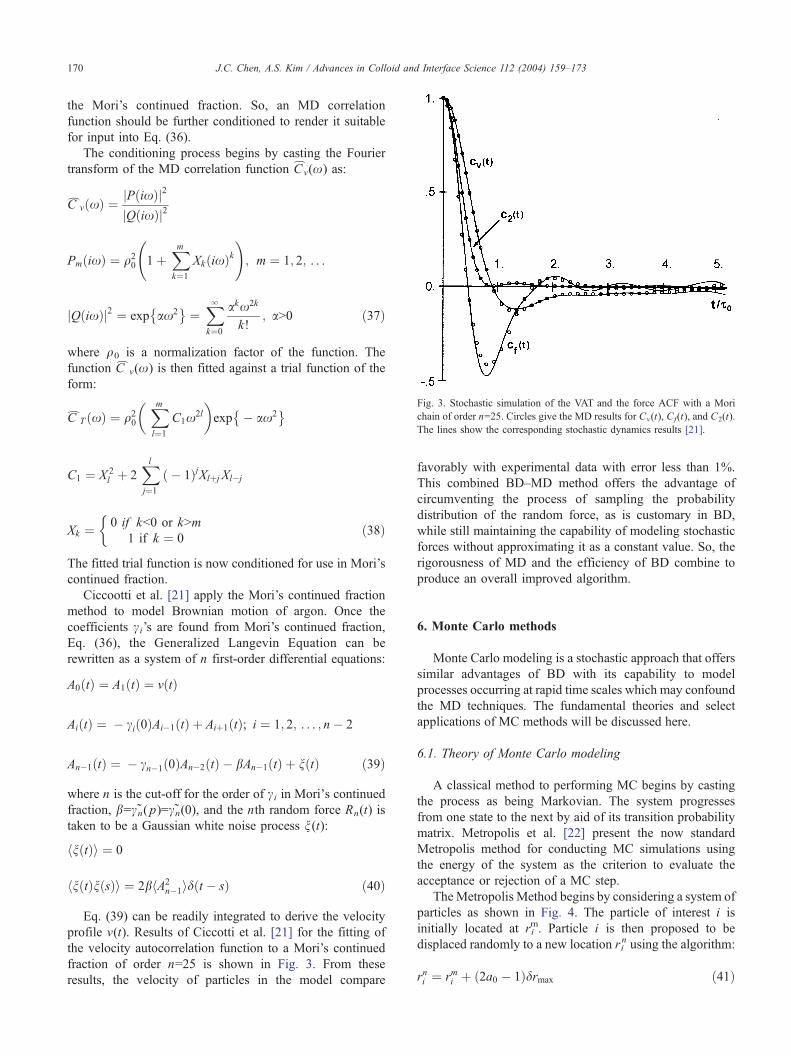
Fig. 3. Stochastic simulation of the VAT and the force ACF with a Mori

chain of order n=25. Circles give the MD results for Cv(t), Cf(t), and C2(t).

The lines show the corresponding stochastic dynamics results [21].

J.C. Chen, A.S. Kim / Advances in Colloid and Interface Science 112 (2004) 159–173170

the Mori’s continued fraction. So, an MD correlation

function should be further conditioned to render it suitable

for input into Eq. (36).

The conditioning process begins by casting the Fourier

transform of the MD correlation function Cf v(x) as:

Cf vðxÞ ¼ jP ixð Þj2

jQ ixð Þj2

Pm ixð Þ ¼ q20 1þ

Xmk¼1

Xk ixð Þk !

; m ¼ 1; 2; . . .

jQ ixð Þj2 ¼ exp ax2

¼Xlk¼0

akx2k

k!; aN0 ð37Þ

where q0 is a normalization factor of the function. The

function Cf v(x) is then fitted against a trial function of the

form:

Cf T ðxÞ ¼ q20

� Xml¼1

C1x2l

�exp � ax2

C1 ¼ X 2l þ 2

Xlj¼1

� 1ð ÞjXlþj Xl�j

Xk ¼0 if kb0 or kNm

1 if k ¼ 0

�ð38Þ

The fitted trial function is now conditioned for use in Mori’s

continued fraction.

Ciccootti et al. [21] apply the Mori’s continued fraction

method to model Brownian motion of argon. Once the

coefficients ci’s are found from Mori’s continued fraction,

Eq. (36), the Generalized Langevin Equation can be

rewritten as a system of n first-order differential equations:

A0 tð Þ ¼ A1 tð Þ ¼ v tð Þ

Ai tð Þ ¼ � ci 0ð ÞAi�1 tð Þ þ Aiþ1 tð Þ; i ¼ 1; 2; . . . ; n� 2

An�1 tð Þ ¼ � cn�1 0ð ÞAn�2 tð Þ � bAn�1 tð Þ þ n tð Þ ð39Þ

where n is the cut-off for the order of ci in MoriTs continuedfraction, b=cn( p)=cn(0), and the nth random force Rn(t) is

taken to be a Gaussian white noise process n(t):

hn tð Þi ¼ 0

hn tð Þn sð Þi ¼ 2bhA2n�1id t � sð Þ ð40Þ

Eq. (39) can be readily integrated to derive the velocity

profile v(t). Results of Ciccotti et al. [21] for the fitting of

the velocity autocorrelation function to a Mori’s continued

fraction of order n=25 is shown in Fig. 3. From these

results, the velocity of particles in the model compare

favorably with experimental data with error less than 1%.

This combined BD–MD method offers the advantage of

circumventing the process of sampling the probability

distribution of the random force, as is customary in BD,

while still maintaining the capability of modeling stochastic

forces without approximating it as a constant value. So, the

rigorousness of MD and the efficiency of BD combine to

produce an overall improved algorithm.

6. Monte Carlo methods

Monte Carlo modeling is a stochastic approach that offers

similar advantages of BD with its capability to model

processes occurring at rapid time scales which may confound

the MD techniques. The fundamental theories and select

applications of MC methods will be discussed here.

6.1. Theory of Monte Carlo modeling

A classical method to performing MC begins by casting

the process as being Markovian. The system progresses

from one state to the next by aid of its transition probability

matrix. Metropolis et al. [22] present the now standard

Metropolis method for conducting MC simulations using

the energy of the system as the criterion to evaluate the

acceptance or rejection of a MC step.

TheMetropolis Method begins by considering a system of

particles as shown in Fig. 4. The particle of interest i is

initially located at rim. Particle i is then proposed to be

displaced randomly to a new location rin using the algorithm:

rni ¼ rmi þ 2a0 � 1ð Þdrmax ð41Þ

Fig. 4. State n is obtained from state m by moving atom i with a uniform

probability to any point in the shaded region R [22].

J.C. Chen, A.S. Kim / Advances in Colloid and Interface Science 112 (2004) 159–173 171

where a0 is a uniform random number between 0 and 1 and

drmax is the maximum allowable displacement. The proposed

displacement is next evaluated for acceptance or rejection.

The criterion for acceptance is the change in potential energy

of the system computed as:

dVn;m ¼XNj¼1

V rni;j

� ��XNj¼1

V rmi;j

� � !ð42Þ

where the potential energy is summed over all the particles

within a cutoff distance rc in relation to particle i. If dVn,mb0,

then the proposedmove is downhill and accepted. If dVn,mN0,

the proposed move is uphill and is accepted with the

qualification of the probability qn/qm which in the Metrop-

olis method corresponds to the Boltzmann factor of the

energy difference:

qn

qm

¼exp � bVnð Þexp � bdVn;m

� �exp � bVnð Þ ¼ exp � bdVn;m

� �ð43Þ

where b=1/kBT. In this procedure, a uniform random number

between 0 and 1, n, is generated and compared with

exp(�bdVn,m). If nbexp(�bdVn,m), then the uphill move is

accepted. Otherwise, the proposed move is rejected for

nNexp(�bdVn,m). The overall effect is that the particle

proceeds with changes in potential energy dVn,m that is

accepted with probability exp(�bdVn,m). If the uphill move

is rejected, the particle remains in its original position, and the

non-move is taken to be a new state nevertheless. The

modeling process continues by randomly selecting succes-

sive particles for proposed displacements. Hastings [23]

presents an improvement by selecting particles systemati-

cally according to their indices rather than by random

selection. This step eases the number of random number

generations. For the Hastings method, an important distinc-

tion should be noted, that is, it does not satisfy detailed

balance. Manousiouthakis and Deem [24] prove that the

Hasting method only satisfies balance. Details of Monte

Carlo modeling are given in Allen and Tildesley [25], Frankel

and Eppenga [26] and Frankel and Ladd [27].

6.2. Application of Monte Carlo methods to Brownian

Dynamics

For physical systems such as protein structures, the

motion of the molecules incurs pronounced time scale

separation between the vibration of bond lengths and bond

angles (on time scale of femtoseconds) versus the torsional

rotation of the molecule (on time scale of nanoseconds). In

these instances a purely BD or MD method meets with the

difficulty of integrating both processes into the model. The

problem arises from the necessities of sampling sufficiently

the conformational space of the molecule and overcoming

the large energy barriers that separate multiple conforma-

tions. For these cases, a method that combines the strengths

of both MC and BD would be capable of overcoming this

dilemma.

Guarnieri [28] applies the Monte Carlo strategy in

conjunction with Brownian Dynamics to derive a dual

deterministic–stochastic model of the conformation of

flexible molecules. The method begins by casting the

particle motion in the presence of a heat bath in the form

of the Langevin Equation:

mdv

dt¼ f x tð Þ½ � þ R tð Þ � mcv ð44Þ

where m is the particle mass, f is the systematic force, c is

the friction coefficient, and R is the random force associated

with the bond length and angle vibrations. The statistical

properties of the random force are:

hR tð ÞR tVð Þi ¼ 2mckTd t � tVð Þ ð45Þ

where d is the Dirac delta function.

Eq. (44) can be integrated to produce expressions for the

displacement and velocity:

x t þ Dtð Þ ¼ x tð Þ 1þ exp � cDtð Þ½ � � x t � Dtð Þexp � cDtð Þ

þ f x tð Þ½ �Dt 1� exp � cDtð Þ½ �mc

þ R1 t; t þ Dtð Þ

þ R1 t; t � Dtð Þexp � cDtð Þ

v t þ Dtð Þ ¼ v tð Þexp cDtð Þ

þ f x tð Þ½ � þ f x t þ Dtð Þ½ �f g 1� exp � cDtð Þ½ �2mc

þ R1 t; t þ Dtð Þ þ R1 t þ Dt; t þ 2Dtð Þ½ �2Dt

þ exp � cDtð Þ½R2 t � Dt; tð Þ þ R2 t; t þ Dtð Þ�2Dt

ð46Þ

J.C. Chen, A.S. Kim / Advances in Colloid and Interface Science 112 (2004) 159–173172

where

R1 t; t þ Dtð Þ ¼ 1

mc

Z tþDt

t

dtVR tVð Þ 1� exp � c tV� tð Þ½ �f g

R2 t; t þ Dtð Þ ¼ 1

mc

Z tþDt

t

dtVR tVð Þ exp � c tV� tð Þ½ � � 1f g

ð47Þ

So, the problem now becomes a matter of Monte Carlo

random samplings of R1 and R2 in Eq. (46) according to

Gaussian distributions. Steps of the algorithm are outlined in

Fig. 5.

Fig. 5. Algorithm for a combined MC–BD method. From Guarnieri [28].

The parameters of the Gaussian distributions used in Fig.

5 are:

d1 ¼kT

mc22cDt � 3þ 4exp � cDtð Þ þ exp 2cDtð Þ½ �

� �1=2

d2 ¼kT

mc2� 2cDt þ 3� 4exp cDtð Þ þ exp 2cDtð Þ½ �

� �1=2

d12 ¼

kT

mc2exp cDtð Þ � 2cDt þ exp � cDtð Þ½ �

d1d2ð48Þ

The method of Guarnieri [28] retains the strength of

BD to accommodate rapidly varying random forces

while offering a simplified numerical algorithm using

MC. A similar procedure is undertaken by Ermak and

Buckholz [3]. Additional examples of applications of the

technique of Guarnieri [28] are given in Williams and

Hall [29], Smart and McCammon [30], and Laakkonen

et al. [31].

7. Concluding remarks

In this review paper, we embark on a sweeping study of

the general theories and algorithms that govern rigorous,

discrete modeling techniques, Brownian Dynamics, Molec-

ular Dynamics and Monte Carlo Methods. At the outset,

we perceived that the capabilities of BD, MD, and MC

methods to discretely model particle trajectories at the

microscopic level cast these methods as potentially more

accurate and robust than the more traditional macroscopic

integral approaches such as the OZ Integral Method with

Hyper-Netter-Chain (HNC) or Percus-Yevick (PY) Clo-

sures. We support our hypothesis by first presenting an

overview of the statistical theories underlying a critical

component of colloidal transport, Brownian motion. Here

we find that the fundamental equations that define random

Brownian motion such as the probability distributions of

particle positioning are especially conducive for modeling

using the statistical elements contained in BD, MD, and

MC methods.

We next proceed with differentiating the three methods

according to the strengths and weaknesses of their theories

and algorithms in relationship to the modeling of the major

factors in colloidal transport, diffusivity and inter-particle

interactions. Previous studies that engage in BD and MD

modeling have shown that the inter-particle interactions play

a crucial determinative role in affecting the accuracy of a

proposed model. So, an important step in the development

of the model involves properly diagnosing the nature of the

inter-particle interactions operating in the system and then

subsequently selecting the appropriate modeling techniques

J.C. Chen, A.S. Kim / Advances in Colloid and Interface Science 112 (2004) 159–173 173

that would be compatible with that situation. In cases of

high particle concentration, the usual pairwise interactions

should be modified to account for contributions from three-

body interactions. Here we review various models for the

inter-particle interactions and their incorporation into the

numerical algorithms.

Furthermore, we find that BD presents itself to be a more

efficient modeling technique over MD because BD effec-

tively accommodates the molecular forces that are not of

significant interest to the problem using a statistically

equivalent random force. The MD method does not contain

such a computation-saving strategy and requires the input of

all forces present in the system regardless of their signifi-

cance to the problem. So, a purely discrete method that

accounts for all forces in the systems remains at present to be

undesirable as it is too computationally intensive. The proper

balance between precisely modeling the relevant compo-

nents of the problem while circumventing such requirements

for the less important components of the problem produces a

most effective model. With that said, we find that further

improvements to the modeling effort can be attained by

combining both BD and MD methods to generate hybrid

techniques such as the Mori’s Continued Fraction.

Our study of Monte Carlo methods reveals similar traits

for this technique as BD. The MC method presents a simpler

algorithm for implementation. In addition, MC incorporates

the additional step of assessing the energy difference in

progressing from one time step to the next step. So here, the

MC method considers the physicality of the process in

conjunction with its statistical properties. Therefore, MC

may offer a more accurate representation of the physical

attributes of the system.

Our findings and discussions contained herein serve as

an introductory effort for integration of microscopic model-

ing techniques of BD, MD, and MC for colloidal systems.

Our continuing research efforts will next build upon this

study with the development of a discrete method of

modeling colloidal transport and testing of the model with

experimental observations.

Acknowledgement

This work was partially supported by the Department

of the Interior, U.S. Geological Survey (grant no.

01HQGR0079), through the Water Resources Research

Center, University of Hawaii at Manoa, Honolulu. This is

contributed paper CP-2004-08 of the Water Resources

Research Center.

References

[1] Wang MC, Uhlenbeck GE. Rev Mod Phys 1945;17:323.

[2] Ermark DL. J Chem Phys 1975;62:4189.

[3] Ermark DL, Buckholz H. J Comp Physiol 1980;35:169.

[4] Van Gunsteren WF, Berendsen HJC. Mol Phys 1982;45:637.

[5] Verlet L. Phys Rev 1967;159:98.

[6] Allen M. Mol Phys 1980;40:1073.

[7] Russel WB, Saville DA, Schowalter WR. Colloidal Dispersions. New

York7 Cambridge Univ. Press; 1989.

[8] Schrodinger E, Kohlrausch F. Physik Zeits 1926;27:306.

[9] Chandrasekhar S. Rev Mod Phys 1943;15:1.

[10] Wu JZ, Bratko D, Blanch HW, Prausnitz JM. J Chem Phys

2000;113:3360.

[11] Turq P, Lantelme F, Levesque D. Mol Phys 1979;37:223.

[12] Lewis JWE, Singer K. J Chem Soc, Faraday Trans 1975;71:41.

[13] Turq P, Lantelme F, Friedman HL. J Chem Phys 1977;66:3039.

[14] Swope WC, Andersen HC, Berens PH, Wilson KR. J Chem Phys

1982;76:637.

[15] Darden T, York D, Pedersen L. J Chem Phys 1993;98:10089.

[16] Essmann U, Perera L, Berkowitz ML, Darden T, Lee H, Pedersen LG.

J Chem Phys 1995;103:8577.

[17] Greengard L, Rokhlin V. J Comput Phys 1987;73:325.

[18] Kubo R. J Phys Soc Jpn 1957;12:570.

[19] Mori H. Prog Theor Phys 1965;33:423.

[20] Ciccotti G, Jacucci G, McDonald IR. J Stat Phys 1979;21:1.

[21] Ciccotti G, Ferrario M, Ryckaert JP. Mol Phys 1982;46:875.

[22] Metropolis N, Rosenbluth AW, Rosenbluth MN, Teller AH, Teller E. J

Chem Phys 1953;21:1087.

[23] Hastings WK. Biometrika 1970;57:97.

[24] Manousiouthakis VI, Deem MW. J Chem Phys 1999;110:2753.

[25] Allen MP, Tildesley DJ. Computer Simulation of Liquids. Oxford

(UK)7 Clarendon Press; 1987.

[26] Frenkel D, Eppenga R. Phys Rev Lett 1982;49:1089.

[27] Frenkel D, Ladd AJC. J Chem Phys 1984;81:3188.

[28] Guarnieri F. J Math Chem 1995;18:25.

[29] Williams DJ, Hall KB. J Phys Chem 1996;100:8224.

[30] Smart JL, McCammon JA. Biopolymers 1999;49:225.

[31] Laakkonen LJ, Guarnieri F, Perlman JHG, Gershengarn MC, Osman

R. Biochemistry 1996;35:7651.