Large Scale Brownian Dynamics of Confined Suspensions of Rigid Particles

Brennan Sprinkle,1 Florencio Balboa Usabiaga,2, 3 Neelesh A. Patankar,1 and Aleksandar Donev2, ∗

1McCormick School of Engineering, Northwestern University, Evanston, IL 60208

2Courant Institute of Mathematical Sciences,

New York University, New York, NY 10012

3Center for Computational Biology, Flatiron Institute,

Simons Foundation, New York 10010, USA

We introduce methods for large scale Brownian Dynamics (BD) simulation of many rigid

particles of arbitrary shape suspended in a fluctuating fluid. Our method adds Brownian

motion to the rigid multiblob method [F. Balboa Usabiaga et al., Communications in Ap-

plied Mathematics and Computational Science, 11(2):217-296, 2016] at a cost comparable to

the cost of deterministic simulations. We demonstrate that we can efficiently generate deter-

ministic and random displacements for many particles using preconditioned Krylov iterative

methods, if kernel methods to efficiently compute the action of the Rotne-Prager-Yamakawa

(RPY) mobility matrix and it “square” root are available for the given boundary conditions.

These kernel operations can be computed with near linear scaling for periodic domains using

the Positively Split Ewald method. Here we study particles partially confined by gravity

above a no-slip bottom wall using a graphical processing unit (GPU) implementation of the

mobility matrix vector product, combined with a preconditioned Lanczos iteration for gener-

ating Brownian displacements. We address a major challenge in large-scale BD simulations,

capturing the stochastic drift term that arises because of the configuration-dependent mo-

bility. Unlike the widely-used Fixman midpoint scheme, our methods utilize random finite

differences and do not require the solution of resistance problems or the computation of the

action of the inverse square root of the RPY mobility matrix. We construct two temporal

schemes which are viable for large scale simulations, an Euler-Maruyama traction scheme

and a Trapezoidal Slip scheme, which minimize the number of mobility solves per time step

while capturing the required stochastic drift terms. We validate and compare these schemes

numerically by modeling suspensions of boomerang shaped particles sedimented near a bot-

tom wall. Using the trapezoidal scheme, we investigate the steady-state active motion in a

dense suspensions of confined microrollers, whose height above the wall is set by a combi-

nation of thermal noise and active flows. We find the existence of two populations of active

particles, slower ones closer to the bottom and faster ones above them, and demonstrate

that our method provides quantitative accuracy even with relatively coarse resolutions of

the particle geometry.

2

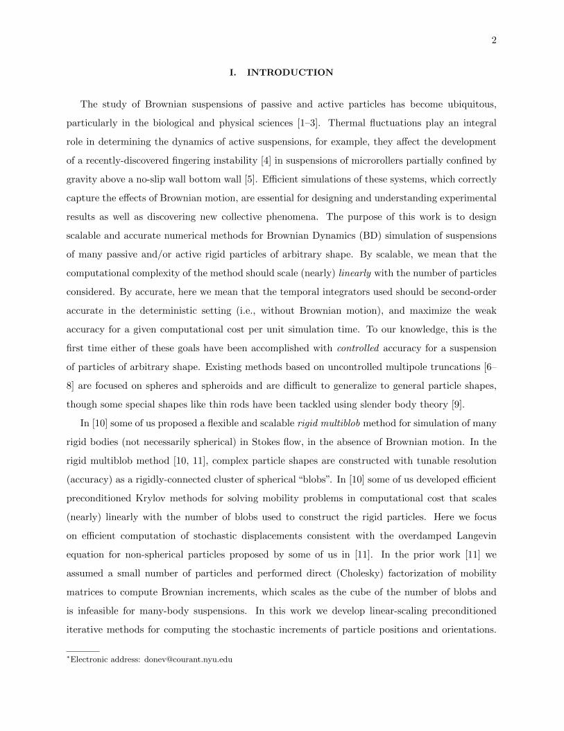
I. INTRODUCTION

The study of Brownian suspensions of passive and active particles has become ubiquitous,

particularly in the biological and physical sciences [1–3]. Thermal fluctuations play an integral

role in determining the dynamics of active suspensions, for example, they affect the development

of a recently-discovered fingering instability [4] in suspensions of microrollers partially confined by

gravity above a no-slip wall bottom wall [5]. Efficient simulations of these systems, which correctly

capture the effects of Brownian motion, are essential for designing and understanding experimental

results as well as discovering new collective phenomena. The purpose of this work is to design

scalable and accurate numerical methods for Brownian Dynamics (BD) simulation of suspensions

of many passive and/or active rigid particles of arbitrary shape. By scalable, we mean that the

computational complexity of the method should scale (nearly) linearly with the number of particles

considered. By accurate, here we mean that the temporal integrators used should be second-order

accurate in the deterministic setting (i.e., without Brownian motion), and maximize the weak

accuracy for a given computational cost per unit simulation time. To our knowledge, this is the

first time either of these goals have been accomplished with controlled accuracy for a suspension

of particles of arbitrary shape. Existing methods based on uncontrolled multipole truncations [6–

8] are focused on spheres and spheroids and are difficult to generalize to general particle shapes,

though some special shapes like thin rods have been tackled using slender body theory [9].

In [10] some of us proposed a flexible and scalable rigid multiblob method for simulation of many

rigid bodies (not necessarily spherical) in Stokes flow, in the absence of Brownian motion. In the

rigid multiblob method [10, 11], complex particle shapes are constructed with tunable resolution

(accuracy) as a rigidly-connected cluster of spherical “blobs”. In [10] some of us developed efficient

preconditioned Krylov methods for solving mobility problems in computational cost that scales

(nearly) linearly with the number of blobs used to construct the rigid particles. Here we focus

on efficient computation of stochastic displacements consistent with the overdamped Langevin

equation for non-spherical particles proposed by some of us in [11]. In the prior work [11] we

assumed a small number of particles and performed direct (Cholesky) factorization of mobility

matrices to compute Brownian increments, which scales as the cube of the number of blobs and

is infeasible for many-body suspensions. In this work we develop linear-scaling preconditioned

iterative methods for computing the stochastic increments of particle positions and orientations.

∗Electronic address: donev@courant.nyu.edu

3

A second nontrivial challenge we address is the construction of consistent and accurate temporal

integrators. The widely-used Fixman midpoint temporal integrator, generalized to include particle

orientations in [11], requires solving resistance problems, which cannot be done in linear time with

present methods [10]. Here we construct two temporal integrators that correctly capture stochastic

drift terms proportional to the divergence of the mobility matrix, and require only solving mobility

problems. While here we only test these novel schemes with the rigid multiblob method [10],

it is important to note that the same temporal integrators apply to highly-accurate boundary

integral formulations [44] for Stokesian suspensions [12–14]. Furthermore, while we focus here on

suspensions confined above a no-slip wall, the methods we present here are rather general and can

be applied to other systems such as bulk passive or active suspensions.

In section II B, we develop a scalable method to generate the Brownian increments for the

particles from the Brownian increments of the individual blobs, which can themselves be computed

using a preconditioned Lanczos method [15], as previously described for particles above a no-slip

wall in [5], and for periodic suspensions in [16]. In section III A we propose a novel modification of

the Euler-Maruyama (EM) scheme, which involves solving only a single additional mobility problem

in order to capture the Ito stochastic (thermal) drift required to maintain the Gibbs-Boltzmann

distribution at equilibrium. This is a notable improvement over the EM method proposed in [11]

which requires two additional mobility solves to compute the drift using a random finite difference

(RFD). In section III B we propose a novel trapezoidal scheme which also captures the correct

thermal drift by solving only a single additional mobility problem, and is second order accurate in

time for deterministic calculations. While the scheme is formally only first-order weakly accurate

in the stochastic setting, the improved deterministic accuracy translates to substantially improved

weak accuracy, as we demonstrate numerically.

In sections IV A 1 and IV B, we validate the new temporal integrators and compare their effi-

ciency/accuracy tradeoffs by examining equilibrium statistics for suspensions of passive colloidal

boomerangs confined above a wall. In section IV C we revisit some experimental and computational

investigations done in [5] for dense uniform suspensions of rotating colloids (microrollers) above a

planar wall. In this prior work [5], a large mismatch was observed between experimental measure-

ments of the steady-state mean suspension velocity and estimates based on the minimally-resolved

Brownian dynamics computations [5]. Here we are able to simulate a dense uniform suspension

of microrollers with much higher resolution. The higher resolution allows us to better resolve

the hydrodynamic interactions between the particles and make quantitative predictions that are

sufficiently accurate to be directly compared to experiments.

4

II. BROWNIAN DYNAMICS FOR RIGID BODIES

We consider a suspension of Nb passive or active rigid bodies (particles) suspended in a fluc-

tuating Stokesian fluid. For body p ∈ [1, . . . , Nb], we will follow a reference tracking point with

Cartesian position, qp (t). The orientation of body p relative to the tracking point will be denoted

by θp (t). For simplicity and increased generality, we make the bulk of the discussion in this work

agnostic to the choice of coordinates for θp and assume that the representation is a scalar in two

dimensions or a three-dimensional vector in three dimensions. In practice, however, we use unit

quaternions in three dimensions, as discussed in detail in [11]. The unit norm constraint of the

quaternion can be handled simply by updating orientation using quaternion multiplication (ro-

tations) instead of addition, as detailed in Appendix B 1. We denote the generalized position of

body p as Qp (t) =[qp (t) ,θp (t)

]and denote the many-body configuration with Q =

[Qp

]. To

each body p, we prescribe an applied force fp, and an applied torque τ p, and denote the gen-

eralized force on body p with F p =[fp, τ p

]and write F = [F p]. The prescription of external

(non-conservative) forces and torques is one way in which we may model active bodies, the other,

active slip, is discussed in more detail in [10] and summarized in section II A.

Given forces and torques, our aim is to find the rigid body velocities U = [Up], where the

generalized velocity Up = [up,ωp] is composed of a translational velocity up and a rotational

(angular) velocity ωp. A central object in the overdamped Langevin equations for the suspension is

the configuration-dependent body mobility matrix N (Q). In a deterministic setting, the symmetric

positive-definite (SPD) matrix N , relates the generalized velocities with the generalized forces,

U = NF . The application of the body mobility matrix, i.e., the computation of U = NF given

F , is referred to as the mobility problem. Its inverse problem, the resistance problem, involves

finding the forces and torques given prescribed rigid-body motions, i.e., computing F = N−1U .

By combining the rigid multiblob method with preconditioned iterative solvers, one can solve a

mobility problem efficiently in linear time, however, the solution of resistance problems is much

more expensive and does not scale linearly [10].

For a suspension of rigid bodies, the configuration evolves according to the overdamped Langevin

Ito BD equation,

dQ

dt= U = NF + kBT (∂Q ·N ) +

√2kBT N 1/2W , (1)

where W is a collection of independent white noise processes [11]. Here the “square root” of

the mobility N 1/2 is any matrix, not necessarily square, that satisfies the fluctuation-dissipation

5

relation N = N 1/2(N 1/2

)T. We will refer to the term kBT ∂Q ·N as the stochastic or thermal

drift (or sometimes simply the drift) since it has its origin in the stochastic interpretation of the

noise; this drift term would disappear if the so-called kinetic or Klimontovich interpretation of the

noise is used [17]. Efficient generation of this term will be the most challenging part of this work and

is discussed in detail in section III. As a prelude, in subsection II A we briefly review the methods

proposed in [10] to efficiently compute the deterministic displacements, NF . Then, in subsection

II B, we propose a scalable iterative method for computing the Brownian displacements over a time

interval ∆t,√

2kBT ∆t N 1/2W , where W is a vector of independent standard Gaussian random

variables.

A. Solving Mobility Problems

We discretize the rigid bodies using a rigid multi-blob model, wherein rigid bodies are treated

as rigid conglomerations of beads, or “blobs”, of hydrodynamic radius a. The blobs comprising a

given rigid body Bp have positions r(p) = [ri | i ∈ Bp]. Given a rigid body velocity Up = [up,ωp],

the geometric block matrix K that converts rigid body motion into blob motion is defined as [18]

(KU)i = up + ωp ×(ri − qp

), p ∈ 1, . . . , NB and i ∈ Bp. (2)

Using K, a slip condition on the rigid bodies can be compactly expressed as

r = KU − u, (3)

where u is a prescribed slip velocity of the fluid at the locations of the blobs. Physically, u could

account for an active boundary layer [8, 19]. However, in this work, we will find a great deal of

utility in prescribing u in such a way as to help generate the stochastic terms in equation (1).

The force and torque balance conditions on the particles can be expressed using the adjoint of K,

KTλ = F [18].

The hydrodynamic interactions between blob i and j are captured by the 3× 3 mobility matrix

M ij , which gives the velocity ri of blob i given a force λj on blob j, ri = M ijλj . The symmetric,

positive semi-definite matrix M composed of the blocks M ij is termed the blob-blob mobility

matrix. The construction of M for a rigid multiblob must account for the finite hydrodynamic

radius of the blobs, a, as well as the geometry of the domain. In the case of a three dimensional

unbounded domain, the well-known Rotne-Prager-Yamakawa (RPY) tensor [20, 21] can be used

to construct M ij , and the action of M on a vector can be computed in linear time using a fast

6

multipole method [22]. For periodic domains, we can use the Positively Split Ewald (PSE) method

[16] to compute the action of the RPY-based mobility M on a vector. A generalization of the RPY

kernel to particles confined above a single no-slip wall, the Rotne-Prager-Blake tensor, is given in

[23] and we will use it in section IV. For general fully-confined domains, an on-the-fly procedure

to calculate M has been proposed in [24, 25]. Note that the action of M can be interpreted as a

physically-regularized single-layer (first-kind) boundary integral operator (see appendix A of [10]).

Given M, we can write the mobility problem as a linear system

Mλ = KU − u (4)

KTλ = F , (5)

which can be written as the saddle-point linear system, M −K

−KT 0

λU

=

−u−F

. (6)

Using Schur complements, we can compactly write the solution to (6) as

U = NF + NKTM−1u, (7)

where we have identified the body mobility matrix

N =(KTM−1K

)−1. (8)

We note that exactly the same saddle-point system, with a mobility matrix M computed using sin-

gular quadratures instead of the RPY kernel, appears in a recently-developed first-kind Fluctuating

Boundary Integral Method (FBIM) for suspensions [26].

In the case of many bodies, computing (the action of) N directly from equation (8) is very

inefficient if at all feasible. In practice, we will solve mobility problems by solving (6) directly.

Efficient, preconditioned Krylov solvers to solve this system were developed in [10]. The efficiency

of these solvers is dependent, primarily, on the speed at which the matrix, M, can be applied to

a vector. If a linear-scaling method such as a fast-multipole-method (FMM) [22, 27] or the PSE

method [16] are used, these methods will scale near linearly (to within logarithmic factors) with

the total number of blobs. Following [10], here we will use direct dense matrix-vector products

implemented on a GPU to apply the Rotne-Prager-Blake mobility. While this in principle scales

quadratically with the total number of blobs, modern GPUs are typically powerful enough for a

direct implementation of a matrix-vector product to outperform more sophisticated techniques up

7

to a fairly large number (hundreds of thousands) of blobs [5]. No matter how fast the matrix-

vector products with N (or equivalently M) can be computed, solving the system (6) is one of

two bottlenecks in designing efficient integrators to solve (1). We discuss the other bottleneck next.

B. Computing Brownian increments

As mentioned in section II A, direct computation of N =(KTM−1K

)−1is computationally

infeasible for many bodies due to the dense matrix inversions required. Direct computation of N 1/2,

therefore, is still less practical in these situations. Our key insight to overcome this is that N 1/2 is

not unique and doesn’t need to be a square matrix, it only needs to satisfy N = N 1/2(N 1/2

)T.

This gives great freedom in choosing N 1/2 so that its action can be computed in linear time. We

will assume here that we were able to efficiently compute Brownian displacements for the individual

blobs, i.e., to compute M1/2W , where W is a vector of independent standard Gaussian random

variables. This can be done using preconditioned iterative methods for bodies near a no-slip wall

[5], using the PSE method [16] for periodic suspensions, or using the FBIM [26] for fully confined

or periodic suspensions.

Let us impose the random slip velocity u =√

2kBT/∆t M1/2W in (6) [45], to get the saddle-

point linear system M −K

−KT 0

λU

=

−√2kBT/∆tM1/2W

0

. (9)

The solution of this system can be written using equation (7) as

U =√

2kBT/∆tNKTM−1M1/2W =√

2kBT/∆tNKTM−1/2W . (10)

It is not hard to see that we can identify the matrix

N 1/2 ≡NKTM−1/2 (11)

as a “square root” of the mobility, since

N 1/2(N 1/2

)T= NKTM−1/2

(M−1/2

)TKN (12)

= N(KTM−1K

)N = NN−1N = N . (13)

Thus, equation (10) becomes

U =

√2kBT

∆tN 1/2W . (14)

8

Hence the Brownian “velocities” (more precisely, the Brownian displacements U∆t) for the rigid

bodies can be computed by solving a mobility problem with random slip given by Brownian ve-

locities for the blobs. Observe that we need only a single application of M1/2 to a vector, and

the solution of a single mobility problem, to compute both the deterministic and the Brownian

increments (but not including the stochastic drift terms yet). Note that the same construction of

N 1/2 is used in the recently-developed FBIM [26], with the slip velocity u interpreted as a random

surface velocity distribution with covariance equal to the Green’s function for periodic Stokes flow

(i.e., the periodic Stokeslet).

Given an efficient routine to compute the product Mλ for a given λ, as discussed in section II A,

a preconditioned Lanczos-type iterative method to compute the product M1/2W was proposed in

[15]. In unbounded or periodic domains the number of iterations increases with the size of M, and

the cost of computing M1/2W is many times than that of computing Mλ. In the PSE method an

additional splitting of M into a near-field and far-field components is introduced, and the Lanczos

method is only applied to the near field, while the far-field component is handled using fluctuating

hydrodynamics. For particles confined close to a no-slip wall, the friction with the floor screens the

hydrodynamic interactions to decay like inverse distance cubed. This makes the Lanczos iteration

converge in a small number of iterations independent of the number of blobs [5]. However, for

rigid multiblobs the number of iterations is higher than for single blobs because of the increased

ill-conditioning of M due to the presence of (nearly-)touching blobs.

In this work, we employ a block diagonal preconditioner M ≈M for the Lanczos algorithm

[15] that substantially reduces the number of iterations in the computation of M1/2W for rigid

multiblobs. Similar block-diagonal or diagonal preconditioners have been used for Stokesian sus-

pensions by other authors [14, 28–31]. In the preconditioner, which is also used to solve the

saddle-point system (6) [10], we ignore hydrodynamic interactions between distinct bodies p and q,

M(pq)

= δpqM(pp). For each body p we explicitly form a dense blob-blob mobility matrix M(pp)

(equal to the diagonal block of M corresponding to body p), ignoring the presence of other bodies.

The preconditioner for the Lanczos method is a block diagonal matrix L = M12 composed of the

Cholesky factors of M(pp). We pre-compute L once per time step (or less frequently if desired)

and then reuse it in the iterative solves in that time step.

In Fig. 1 we probe the convergence of our preconditioned solvers in a suspension of boomerang

colloidal particles sedimented over a rigid wall for surface area fraction φ ≈ 0.25 (see details in Sec.

IV). The figure shows the number of iterations required to reach a desired tolerance for both the

solution of (6), as well as for computing the product M1/2W , for three different problem sizes.

9

0 10 20 30 40 50iteration

10-6

10-5

10-4

10-3

10-2

10-1

100

Rel

ativ

e re

sidual

Nb = 256

Nb = 1024

Nb = 4096

Nb = 256

Nb = 1024

Nb = 4096

Nb = 256

Nb = 1024

Nb = 4096

}}}

Rigid solve

PC Lanczos

un-PC Lanczos

Figure 1: Convergence of iterative solvers for the problem described in section IV B, a suspension of 256,

1024 or 4096 colloidal boomerangs (each containing 15 blobs) sedimented near a bottom wall. Convergence

of the preconditioned GMRES iteration to solve equation (6), labeled as ‘Rigid solve’, is demarcated by solid

lines. Convergence of the preconditioned Lanczos method to compute M1/2W , labeled as ’PC Lanczos’,

is demarcated by filled symbols, while the corresponding results without preconditioning, labeled as ’un-PC

Lanczos’, are demarcated by un-filled symbols.

Also shown is the effect of preconditioning on the convergence of the matrix root computation. We

can see that up to a relative tolerance of around 10−3, both the saddle point solve, (6) and M1/2W

require roughly the same number of iterations to converge, with the latter taking more iterations

when smaller tolerances are required. When preconditioning is used, both iterative methods are

shown to have convergence rates independent of problem size. Nevertheless, computing matrix

roots represents another major bottleneck in integrating (1) for rigid multiblobs confined above a

no-slip floor, with cost similar to that of solving the saddle point system (6). Observe that both

the computation of the deterministic and the fluctuating velocities involves repeated applications

of M, which dominates the cost. Therefore, we seek to integrate (1) to a desired accuracy in as

few total number of applications of M as possible.

10

III. TEMPORAL INTEGRATORS AND THE THERMAL DRIFT

Our goal is to numerically integrate the overdamped Langevin equation (1) as efficiently as

possible. In section II we discussed efficient means of computing NF +√

2kBT/∆t N 1/2W , all

that remains is to find a way to efficiently generate the thermal drift term kBT ∂Q ·N . Capturing

this drift term is a common challenge in all methods for Brownian dynamics, and the methods

developed here are general and apply to any approach based on solving mobility problems.

A widely-used method to capture kBT ∂Q · N is due to Fixman [32], and can be seen as a

midpoint method to capture the Stratonovich product in a mixed Stratonovich-Ito (also known as

Klimontovich or kinetic interpretation [17]) re-formulation of (1) [11]. The generalization of Fix-

man’s method to account for particle orientations is given in Section III of [11]. The problem with

the Fixman scheme in the context of many-body suspensions is that it requires the computation

of N−1/2W . This is related to solving resistance problems and is infeasible for many body simu-

lations. In particular, there is no known method to compute M−1 which scales linearly with the

problem size. Hence, the Fixman’s scheme has to be ruled out for use in many body simulations.

Here we will only use Fixman’s method as a reference method for small problems involving at most

on the order of a hundred blobs, where dense linear algebra is practicable [11].

In [11, 33], some of us proposed a means of capturing the drift term in (1) using a modification

of Fixman’s approach. This idea, termed random finite difference (RFD), is as follows. Given two

Gaussian random vectors, ∆P and ∆Q, such that⟨∆P∆QT

⟩= (kBT ) I, the following relation

holds for a configuration dependent matrix B (Q),

limδ→0

1

δ〈{B (Q+ δ∆Q)−B (Q)}∆P 〉 = (15)

limδ→0

1

δ

⟨{B(Q+

δ

2∆Q

)−B

(Q− δ

2∆Q

)}∆P

⟩= (16)

{∂QB (Q)} :⟨∆P∆QT

⟩= kBT ∂Q ·B (Q) , (17)

where 〈〉 denotes an ensemble average. In practice, we will implement random finite differences

by simply taking δ to be a small number. Thus we recognize, by analogy with standard finite

differences, equations (15) and (16) as one-sided and centered approximations to (17) with trun-

cation errors of O (δ) and O(δ2)

respectively. Note that Fixman’s scheme can be viewed as an

RFD where δ =√

∆t, B = N , ∆Q =√kBTN 1/2W , and ∆P =

√kBTN−1/2W [33]; see Sec-

tion III.D in [6] for the first use of a δ independent of ∆t in order to “avoid particle ’overlaps’

in the intermediate configuration.” A simpler choice, used in [5, 11], is to take B = N , and use

∆P = ∆Q =√kBTW . Other more efficient choices have been constructed in a number of specific

11

contexts [7, 24, 34]. In order to best pick δ, we must balance the truncation error with other sources

of error introduced from the inexact multiplication of B. At best, multiplication by B is calculated

to machine precision and δ may be taken to be quite small. At worst, multiplication of B is only

computed approximately to within some relative tolerance ε, as would be the case when we take

B = N and matrix vector multiplications are computed using the iterative method described in

section (II A). In this case, using one-sided differencing can lead to large truncation errors when

loose solver tolerances are used, and we recommend that only central differencing be used.

In [11], an Euler-Maruyama (EM) RFD (EM-RFD) scheme is presented to solve (1), using

a one-sided RFD on N . A scalable variant of this using a central RFD is a trivial extension

summarized in appendix A, where we clarify how to do this using iterative solvers and also with

care for different units for length and orientation. This scheme requires three solutions of the saddle

point system (6) and one application of M1/2 per timestep, and is only first-order accurate even

deterministically. By using different choices for ∆P and ∆Q in (16), we will reduce the cost of

capturing the stochastic drift term considerably. In section III A we will present an EM Traction

(EM-T) scheme which only requires two solutions of the saddle point system. The trapezoidal slip

(T-S) scheme presented in section III B still requires three solutions of the saddle point system but

achieves higher accuracy, notably, it is second-order accurate deterministically just like the Fixman

midpoint scheme given in [11]. We will empirically compare these two schemes in terms of accuracy

per computational effort in Section IV B.

A. Euler-Maruyama Traction (EM-T) Scheme

To improve the efficiency of the scheme given in appendix A, we propose a different means of

computing the drift term. Using the chain rule, we can split the divergence of the body mobility

matrix into three pieces,

∂Q ·N = −N(∂QN−1

): N = −N

(∂Q{KTM−1K

}): N = (18)

−N{∂QKT

}: M−1KN −NKT

{∂QM−1

}: KN −NKTM−1 {∂QK} : N =

−N{∂QKT

}: M−1KN + NKTM−1 {∂QM} : M−1KN −NKTM−1 {∂QK} : N .

where colon denotes contraction; this calculation is done more precisely using index notation in

appendix B 1. Unlike N , we can efficiently compute the action of KT , M, and K, without the

need for a linear solver [46]. Thus, we can use a random finite difference to compute the three

derivatives ∂QKT , ∂QM, and ∂QK in equation (18) separately. When selecting the value of δ

12

for these computations, we must balance the truncation error of the RFD (we will only consider

centered differences) with the relative accuracy in computing the product of the operator (i.e K,

M). If the matrix-vector products are computed directly, then we balance the truncation error

with the machine precision and take δ ∼ 10−3 when single precision is used [47], and δ ∼ 10−6 for

double precision. However, if we only compute the action of M to within some relative accuracy

ε, as would be the case if we used the FMM or PSE method, we must take δ ∼ ε1/3.

To utilize equation (18), we first generate random forces and torques for each body p

W FTp = kBT

L−1p W

fp

W τp

, (19)

where W fp , W

τp are standard Guassian random vectors, and Lp is a measure of the body length.

Note the choice of length scale used in the blocks of (19) is to minimize the variance of the RFD

estimate, as we explain in appendix A. We then solve a mobility problem with random applied

forces and torques W FT =[W FT

p

], for both the random traction force λRFD, and the random

rigid velocity URFD,

λRFD = M−1KN W FT (20)

URFD = N W FT . (21)

To compute the relevant random finite difference terms, we randomly displace the particles to Q±,

where

Q±p = Qp ±δ

2∆Qp = Qp ±

δ

2

LpW fp

W τp

. (22)

Using this and equation (18), we are able to compute the necessary drift term using random finite

differences as

Drift =− 1

δN{KT (Q+)−KT (Q−)

}λRFD (23)

+1

δNKTM−1

{M(Q+)−M(Q−)

}λRFD

− 1

δNKTM−1

{K(Q+)−K(Q−)

}URFD

≈(−N

{∂QKT

}M−1KN

+ NKTM−1 {∂QM}M−1KN

−NKTM−1 {∂QK}N)

:[W FT (∆Q)T

]=∂QN :

[W FT (∆Q)T

],

13

where all operators and derivatives are evaluated at the same point Q unless otherwise noted and

(∆Q)T denotes the transpose of ∆Q. Hence, in expectation, we have

〈Drift〉 ≈ kBT ∂Q ·N . (24)

This computation is detailed in index notation, accounting for the constrained quaternion repre-

sentation of orientations, in Appendix B 2.

To leading order in δ, the method of computing the drift proposed in equation (23), termed

the traction-corrected RFD, is equivalent to the direct RFD on N used in appendix A when

exact linear algebra is used. However, using the traction-corrected RFD allows the use of inexact,

iterative mobility solvers, without incurring additional restrictions on the small parameter δ from

the prescribed solver tolerance. Furthermore, we are able to capture the drift term in equation

(1) with only two saddle point solves rather than the three required if we were to use an RFD on

N directly. Our Euler-Maruyama Traction (EM-T) Scheme is summarized in algorithm 1, and is

analyzed in Appendix B 2.

B. Trapezoidal Slip (T-S) Scheme

In section III A, we developed a method to efficiently and accurately generate the necessary

drift term in an Euler-Maruyama scheme. However, when second order deterministic accuracy is

desired, we may wish to use a midpoint or trapezoidal scheme [33]. Some higher order methods,

however, will generate additional drift terms due to the Brownian increment being evaluated at

multiple time levels. As an example, consider a naive two-solve implementation of the trapezoidal

scheme:

Q =Qn + ∆tN nF n +√

2∆tkBT(NKTM−1

)n (M1/2)n W n (25)

Qn+1 =Qn +∆t

2

(N nF n + N F

)(26)

+

√∆tkBT

2

{(NKTM−1

)n+ N K

TM−1}(

M1/2)n W n,

where superscripts and tildes indicate the point at which quantities are evaluated, e.g., N ≡

N(Q)

.

As shown in Appendix B 3, the thermal drift produced by the final velocity update in equation

(26) (in expectation) is

〈Drift part 1〉 =

⟨Qn+1 −Qn

∆t

⟩≈ (kBT ) NKTM−1 {∂QK} : N , (27)

14

Algorithm 1 Euler-Maruyama Traction (EM-T) Scheme

1. Compute relevant quantities for capturing drift:

(a) Form W FT =[W FT

p

], where

W FTp = kBT

L−1p W

fp

W τp

and W f

p , Wτp are standard Gaussian random vectors.

(b) Solve RFD mobility problem: Mn −Kn

−(KT)n

0

λRFD

URFD

=

0

−W FT

.(c) Randomly displace particles to:

Q±p = Qn

p +δ

2

LpW fp

W τp

.(d) Compute the force-drift, DF , and the slip-drift, DS :

DF =1

δ

{KT

(Q+)−KT

(Q−)}λRFD

DS =1

δ

{M(Q+)−M

(Q−)}λRFD − 1

δ

{K(Q+)−K

(Q−)}URFD.

Note that different δ may be used for the RFDs on K and M depending on the relative accuracy

with which the action of M is evaluated.

2. Compute(M1/2

)nW n using a preconditioned Lancoz method or PSE.

3. Evaluate forces and torques at F n = F (Qn, t) and solve the mobility problem: Mn −Kn

−(KT)n

0

λnUn

=

−DS −√

2kBT/∆t(M1/2

)nW n

−F n +DF

.4. Update configurations to time t+ ∆t:

Qn+1 = Qn + ∆tUn.

We recognize this as the third term in equation (18) and hence, we may use it to generate the full,

desired drift. Examining equation (18) reveals that we must generate the remaining two terms

−N{∂QKT

}: M−1KN + NKTM−1 {∂QM} : M−1KN , (28)

15

in order to capture the desired drift.

In section III A, we generated random traction forces of the form M−1KNW FT , and used

these as the ∆P in equation (17) to compute a traction-corrected RFD approximation to (28).

Here we propose a different slip-corrected RFD method to compute the two terms in (28). For each

body, we generate a vector of random blob displacements WD

=[LpW

sp

], and random blob forces

WF

=[kBTLpW s

p

], where Lp is a length scale for body p, and W s is a random Gaussian vector.

We may then compute rigid body displacements, ∆QRFD = NKTM−1WD

, which may be used

as ∆Q in equation (17) to compute an RFD approximation to (28). That is, we may approximate

the missing drift terms (28) by computing

Drift part 2 =− 1

δN{KT (Q+)−KT (Q−)

}W

F(29)

+1

δNKTM−1

{M(Q+)−M(Q−)

}W

F

≈(−N

{∂QKT

}+ NKTM−1 {∂QM}

):[W

F (∆QRFD

)T ]= (kBT )

(−N

{∂QKT

}+ NKTM−1 {∂QM}

): M−1KN

[W s (W s)T

],

where as before Q±p = Qp ± δ2∆QRFD

p . Hence, in expectation we obtain the missing drift terms

(28),

〈Drift part 2〉 ≈ kBT(−N

{∂QKT

}: M−1KN + NKTM−1 {∂QM} : M−1KN

),

which combined with (27) gives us the desired drift kBT ∂Q ·N .

Our Trapezoidal Slip (T-S) scheme is summarized in algorithm 2, and is analyzed in Appendix

B 3. It involves three mobility solves and one Lanczos computation per time step, just like the

EM-RFD scheme given in Algorithm 3, however, T-S is second order deterministically just like the

Fixman midpoint scheme.

It is important to point out that by using either the traction-corrected RFD (i.e., applying

random uncorrelated forces and torques on the particles) or the slip-corrected RFD (i.e., applying

random uncorrelated slip on the particles’ surfaces), one can construct a multitude of schemes that

give the desired stochastic drift term in expectation for sufficiently small ∆t. For example, an

alternative method to generate the remaining drift terms in (28), while still using the trapezoidal

rule, would be to compute DS and DF analogous to step 1 of algorithm 1 but without the term

involving URFD (which is already included via the trapezoidal corrector step). In numerical tests,

we have found such a Trapezoidal Traction (T-T) scheme to perform very similarly to the (T-S)

16

Algorithm 2 Trapezoidal Slip (T-S) scheme

1. Compute relevant quantities for capturing drift:

(a) Generate random Gaussian directions W s for each blob, and form the composite vectors of

blob displacements WD

=[LpW

sp

]and blob forces W

F=[kBTLpW s

p

].

(b) Solve RFD mobility (more precisely, displacement) problem: Mn −Kn

−(KT)n

0

λRFD

∆QRFD

=

−WD

0

.(c) Randomly displace particles to Q±:

Q± = Qn ± δ

2∆QRFD

(d) Compute the force-drift, DF , and the slip-drift, DS , where:

DF =1

δ

{KT

(Q+)−KT

(Q−)} W F

,

DS =1

δ

{M(Q+)−M

(Q−)} W F

.

Note that different δ may be used for the two RFDs depending on the relative accuracy with

which the action of M is evaluated.

2. Compute(M1/2

)nW n using a preconditioned Lancoz method or PSE.

3. Evaluate forces and torques at F n = F (Qn, t) and solve predictor mobility problem: Mn −Kn

−(KT)n

0

λnUn

=

−√2kBT/∆t(M1/2

)nW n

−F n

.4. Update configurations to predicted position Q:

Q = Qn + ∆tUn.

5. Evaluate forces and torques at F = F(Q, t

)and solve corrector mobility problem at the predicted

position Q: M −K

−KT

0

λU

=

−2DS −√

2kBT∆t (M1/2)nW n

−F + 2DF

.6. Update configurations to corrected position Qn+1:

Qn+1 = Qn +∆t

2

(Un + U

).

17

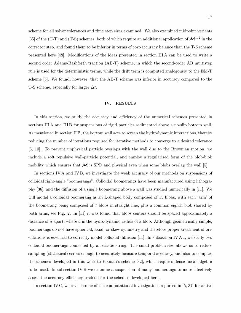
scheme for all solver tolerances and time step sizes examined. We also examined midpoint variants

[35] of the (T-T) and (T-S) schemes, both of which require an additional application of M1/2 in the

corrector step, and found them to be inferior in terms of cost-accuracy balance than the T-S scheme

presented here [48]. Modifications of the ideas presented in section III A can be used to write a

second order Adams-Bashforth traction (AB-T) scheme, in which the second-order AB multistep

rule is used for the deterministic terms, while the drift term is computed analogously to the EM-T

scheme [5]. We found, however, that the AB-T scheme was inferior in accuracy compared to the

T-S scheme, especially for larger ∆t.

IV. RESULTS

In this section, we study the accuracy and efficiency of the numerical schemes presented in

sections III A and III B for suspensions of rigid particles sedimented above a no-slip bottom wall.

As mentioned in section II B, the bottom wall acts to screen the hydrodynamic interactions, thereby

reducing the number of iterations required for iterative methods to converge to a desired tolerance

[5, 10]. To prevent unphysical particle overlaps with the wall due to the Brownian motion, we

include a soft repulsive wall-particle potential, and employ a regularized form of the blob-blob

mobility which ensures that M is SPD and physical even when some blobs overlap the wall [5].

In sections IV A and IV B, we investigate the weak accuracy of our methods on suspensions of

colloidal right-angle ”boomerangs”. Colloidal boomerangs have been manufactured using lithogra-

phy [36], and the diffusion of a single boomerang above a wall was studied numerically in [11]. We

will model a colloidal boomerang as an L-shaped body composed of 15 blobs, with each ‘arm’ of

the boomerang being composed of 7 blobs in straight line, plus a common eighth blob shared by

both arms, see Fig. 2. In [11] it was found that blobs centers should be spaced approximately a

distance of a apart, where a is the hydrodynamic radius of a blob. Although geometrically simple,

boomerangs do not have spherical, axial, or skew symmetry and therefore proper treatment of ori-

entations is essential to correctly model colloidal diffusion [11]. In subsection IV A 1, we study two

colloidal boomerangs connected by an elastic string. The small problem size allows us to reduce

sampling (statistical) errors enough to accurately measure temporal accuracy, and also to compare

the schemes developed in this work to Fixman’s scheme [32], which requires dense linear algebra

to be used. In subsection IV B we examine a suspension of many boomerangs to more effectively

assess the accuracy-efficiency tradeoff for the schemes developed here.

In section IV C, we revisit some of the computational investigations reported in [5, 37] for active

18

suspensions of rotating colloids [4, 37]. In these suspensions thermal motion sets the equilibrium

gravitational height of the colloids, and it is necessary to include Brownian motion to enable

quantitative comparisons to experiments [5, 37]. At the same time, previous studies [5, 37] used

a minimally-resolved representation of the hydrodynamics, with each particle represented by a

single blob. This is not quantitatively accurate when the microrollers are close to the wall or other

colloids, as in recent experiments [4, 37]. We represent the spheres using either 12 or 42 blobs

[10] in order to improve the accuracy of the hydrodynamic interactions, and choose a as roughly

half the distance between vertices in the multiblob sphere model following the recommendations

in Sections IV and V of [10].

Figure 2: Illustrations of the test problems involving colloidal boomerangs. (Top panel) Sample configuration

of a boomerang dimer for the numerical experiments conducted in section IV A 1. (Bottom panel) Sample

configuration of a boomerang suspension for the numerical experiments conducted in section IV B. The

shaded area is the part of the bottom wall that belongs to the central unit cell used for the pseudo-periodic

boundary conditions.

19

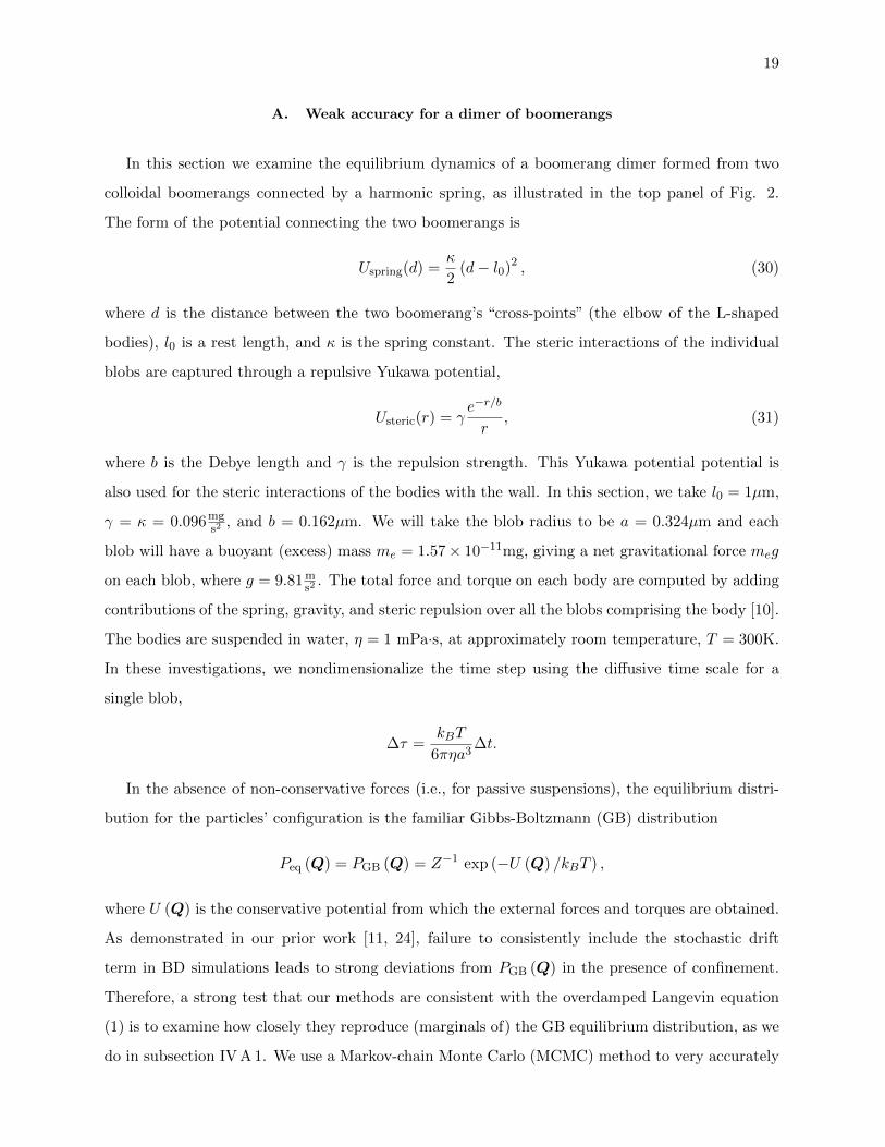
A. Weak accuracy for a dimer of boomerangs

In this section we examine the equilibrium dynamics of a boomerang dimer formed from two

colloidal boomerangs connected by a harmonic spring, as illustrated in the top panel of Fig. 2.

The form of the potential connecting the two boomerangs is

Uspring(d) =κ

2(d− l0)2 , (30)

where d is the distance between the two boomerang’s “cross-points” (the elbow of the L-shaped

bodies), l0 is a rest length, and κ is the spring constant. The steric interactions of the individual

blobs are captured through a repulsive Yukawa potential,

Usteric(r) = γe−r/b

r, (31)

where b is the Debye length and γ is the repulsion strength. This Yukawa potential potential is

also used for the steric interactions of the bodies with the wall. In this section, we take l0 = 1µm,

γ = κ = 0.096mgs2

, and b = 0.162µm. We will take the blob radius to be a = 0.324µm and each

blob will have a buoyant (excess) mass me = 1.57× 10−11mg, giving a net gravitational force meg

on each blob, where g = 9.81 ms2

. The total force and torque on each body are computed by adding

contributions of the spring, gravity, and steric repulsion over all the blobs comprising the body [10].

The bodies are suspended in water, η = 1 mPa·s, at approximately room temperature, T = 300K.

In these investigations, we nondimensionalize the time step using the diffusive time scale for a

single blob,

∆τ =kBT

6πηa3∆t.

In the absence of non-conservative forces (i.e., for passive suspensions), the equilibrium distri-

bution for the particles’ configuration is the familiar Gibbs-Boltzmann (GB) distribution

Peq (Q) = PGB (Q) = Z−1 exp (−U (Q) /kBT ) ,

where U (Q) is the conservative potential from which the external forces and torques are obtained.

As demonstrated in our prior work [11, 24], failure to consistently include the stochastic drift

term in BD simulations leads to strong deviations from PGB (Q) in the presence of confinement.

Therefore, a strong test that our methods are consistent with the overdamped Langevin equation

(1) is to examine how closely they reproduce (marginals of) the GB equilibrium distribution, as we

do in subsection IV A 1. We use a Markov-chain Monte Carlo (MCMC) method to very accurately

20

sample the GB equilibrium distribution and use this data to compute the error produced by each

scheme. At the same time, it is important to also confirm that our schemes, unlike MCMC,

correctly reproduce the dynamics of the particles even for time steps that are on the order of the

diffusive time scale, as we do in subsection IV A 2.

1. Static Accuracy

The stability limit for the EM-T scheme for the chosen parameters was empirically estimated to

be ∆τ . 0.3. In Figure 3 we study how well our numerical methods reproduce selected the Gibbs-

Boltzmann equilibrium distribution for ∆τ = 0.072, 0.144, 0.288. We have examined a number of

marginals of the equilibrium distribution, but we focus here on the equilibrium distributions of the

boomerang cross-point to cross-point distance. We use a relative tolerance of 10−4 in all iterative

methods for the computations done in this section. An investigation into the effect of solver

tolerance on the accuracy of the EM-T and T-S schemes showed no change in temporal accuracy

for all solver tolerances less than or equal to 10−3, and overall accuracy was only slightly affected

for solver tolerances 10−3 − 10−2, but then degraded rapidly for looser tolerances. Note however,

that using the same solver tolerance for all iterative methods is perhaps not necessary to maintain

temporal accuracy, and looser tolerances may be used for the RFD-related linear solves. We take

the random finite difference parameter δ = 10−6 for both schemes as double precision was used

for these calculations. Results were obtained by averaging 20 independent realizations containing

105 samples, initialized from unique configurations sampled from the equilibrium distribution using

the MCMC algorithm. In addition to the proposed EM-T and T-S schemes, we also compare with

Fixman’s scheme given in Section III.B of [24], implemented using dense linear algebra.

Figure 3 shows that even for the smallest time step size considered, the T-S scheme is substan-

tially more accurate than the EM-T scheme. Note that no data is included for Fixman’s scheme

for the largest time step size considered, because the scheme was seen to be numerically unstable.

While all of the schemes are seen to be O(∆t) in the cummulative L2 error, the order constant for

the T-S and Fixman schemes are clearly much lower than the EM scheme. In terms of accuracy

alone, the T-S scheme compares very favorably with Fixman’s scheme, while also enabling scalable

computations for suspensions of many rigid bodies.

21

Figure 3: Numerical errors in the equilibrium distribution for a boomerang dimer. (Upper left panel)

Comparison between the correct (marginal of the) Gibbs-Boltzmann distribution of the cross-point distance,

computed using an MCMC method, and numerical results from the T-S and EM-T schemes for normalized

time step size ∆τ = 0.072. (Upper right panel) Cumulative error in the distribution of the cross-point

distance, as measured by the L2 norm of the error in the histogram P (d), for the EM-T, T-S and Fixman

schemes. (Lower panels) Error in the distribution of the cross-point distance for the EM-T (left panel),

T-S (middle panel), and the Fixman scheme (right panel) for several different time step sizes (see legend).

Note that the scale of the plots changes and that the Fixman scheme is unstable for ∆τ > 0.29. Error bars

indicate 95% confidence intervals and are estimated from multiple independent runs.

2. Dynamic Accuracy

We now turn our attention to time-dependent statistics by examining the equilibrium transla-

tional mean squared displacement (MSD) of the cross point of one of the two connected boomerangs,

D(t) = 〈∆qp(t)(∆qp(t)

)T 〉 = 〈(qp(t)− qp(0)

) (qp(t)− qp(0)

)T 〉,where the average is an ensemble average over equilibrium trajectories and p = 1 or p = 2. Since

the trajectories of the two boomerangs are statistically identical, we will average results over the

two particles to improve statistical accuracy. Here and in what follows we will assume that the

cross point is chosen as the tracking point around which the boomerang rotates. We may define

22

short-time and long-time translational diffusion tensors,

χst =1

2limt→0

D(t)

t, χlt =

1

2limt→∞

D(t)

t(32)

respectively. The Stokes-Einstein relationship implies

χst = (kBT )⟨N (tt)

pp

⟩GB

, (33)

where we have taken an average over the Gibbs-Boltzmann distribution of the 3 × 3 translation-

translation diagonal block of the mobility matrix corresponding to body p. However, χlt admits no

such simple characterizations and is typically challenging to compute accurately, requiring many

samples from long simulations, as discussed extensively in [11].

Since we are investigating diffusion near an infinite wall (placed at z = 0 with normal in

the positive z direction), under the influence of gravity, we may define the parallel (D‖p) and

perpendicular (D⊥p ) MSD of body p as

D‖p(t) =Dxx(t) +Dyy(t), D⊥p (t) = Dzz(t). (34)

At long times the perpendicular MSD D⊥p (t) asymptotically tends towards a finite value, related

to the gravitational height of the body [11]. We focus here on the parallel MSD D‖p(t) as this is

typically what is measured in experiments [36, 38].

At short times, we can use the Stokes-Einstein formula D‖p(t) = 2 (kBT )

⟨N (xx)

11

⟩GB

t to validate

our simulations. To estimate the long-time MSD, we use a non-equilibrium method based on linear

response theory [39]. Specifically, if we pull one of the boomerangs with a force F = F x applied

to the cross (tracking) point,

〈xp(t)− xp(0)〉F = − F

kBT

∫ t

0

⟨xp(0)xp(t− t′)

⟩0

dt′ =F

2kBT

⟨(xp(t)− xp(0))2

⟩0. (35)

Here the average on the left hand side is an average over nonequilibrum trajectories initialized

from the GB distribution, while the average on the right hand side is an average over equilibrium

trajectories. The formula (35) relates the MSD at equilibrium with the mean displacement under

a external force. The nonequilibrium method offers better statistical accuracy at long times over

computing the MSD if the applied force F is sufficiently large but still small enough to remain in the

linear-response regime (for the simulations reported below the Peclet number is Pe = LF/ (kBT ) ≈

0.5, where L = 2.1µm is the boomerang arm length). To see this, consider a one dimensional

diffusion process with constant mobility µ,

dx(t)

dt= µF +

√2kBTµW(t),

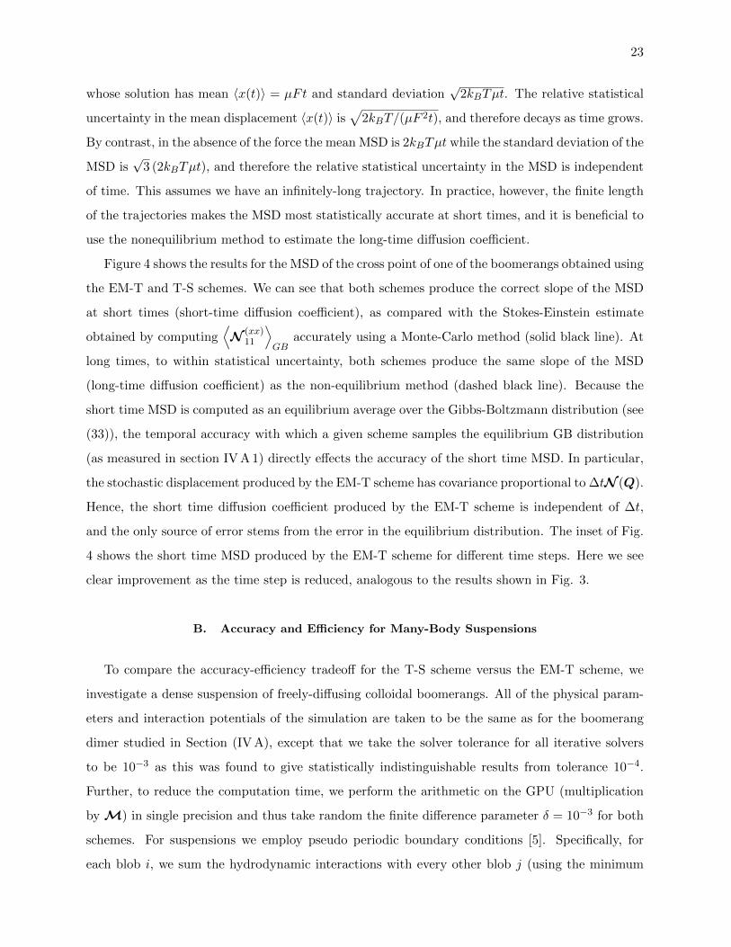
23

whose solution has mean 〈x(t)〉 = µFt and standard deviation√

2kBTµt. The relative statistical

uncertainty in the mean displacement 〈x(t)〉 is√

2kBT/(µF 2t), and therefore decays as time grows.

By contrast, in the absence of the force the mean MSD is 2kBTµt while the standard deviation of the

MSD is√

3 (2kBTµt), and therefore the relative statistical uncertainty in the MSD is independent

of time. This assumes we have an infinitely-long trajectory. In practice, however, the finite length

of the trajectories makes the MSD most statistically accurate at short times, and it is beneficial to

use the nonequilibrium method to estimate the long-time diffusion coefficient.

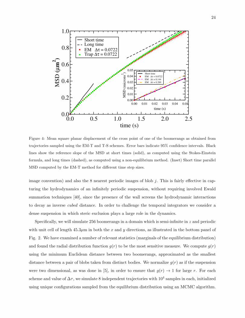
Figure 4 shows the results for the MSD of the cross point of one of the boomerangs obtained using

the EM-T and T-S schemes. We can see that both schemes produce the correct slope of the MSD

at short times (short-time diffusion coefficient), as compared with the Stokes-Einstein estimate

obtained by computing⟨N (xx)

11

⟩GB

accurately using a Monte-Carlo method (solid black line). At

long times, to within statistical uncertainty, both schemes produce the same slope of the MSD

(long-time diffusion coefficient) as the non-equilibrium method (dashed black line). Because the

short time MSD is computed as an equilibrium average over the Gibbs-Boltzmann distribution (see

(33)), the temporal accuracy with which a given scheme samples the equilibrium GB distribution

(as measured in section IV A 1) directly effects the accuracy of the short time MSD. In particular,

the stochastic displacement produced by the EM-T scheme has covariance proportional to ∆tN (Q).

Hence, the short time diffusion coefficient produced by the EM-T scheme is independent of ∆t,

and the only source of error stems from the error in the equilibrium distribution. The inset of Fig.

4 shows the short time MSD produced by the EM-T scheme for different time steps. Here we see

clear improvement as the time step is reduced, analogous to the results shown in Fig. 3.

B. Accuracy and Efficiency for Many-Body Suspensions

To compare the accuracy-efficiency tradeoff for the T-S scheme versus the EM-T scheme, we

investigate a dense suspension of freely-diffusing colloidal boomerangs. All of the physical param-

eters and interaction potentials of the simulation are taken to be the same as for the boomerang

dimer studied in Section (IV A), except that we take the solver tolerance for all iterative solvers

to be 10−3 as this was found to give statistically indistinguishable results from tolerance 10−4.

Further, to reduce the computation time, we perform the arithmetic on the GPU (multiplication

by M) in single precision and thus take random the finite difference parameter δ = 10−3 for both

schemes. For suspensions we employ pseudo periodic boundary conditions [5]. Specifically, for

each blob i, we sum the hydrodynamic interactions with every other blob j (using the minimum

24

0.0 0.5 1.0 1.5 2.0 2.5time (s)

0.0

0.2

0.4

0.6

0.8

1.0

MS

D (

µm

2)

Short timeLong time

EM ∆τ = 0.0722Trap ∆τ = 0.0722

0.00 0.01 0.02 0.03 0.04 0.05

time (s)

0.00

0.01

0.02

0.03

0.04

0.05

MS

D (

mic

ron

s2) Short time

EM ∆τ = 0.0722

EM ∆τ = 0.144

EM ∆τ = 0.289

Figure 4: Mean square planar displacement of the cross point of one of the boomerangs as obtained from

trajectories sampled using the EM-T and T-S schemes. Error bars indicate 95% confidence intervals. Black

lines show the reference slope of the MSD at short times (solid), as computed using the Stokes-Einstein

formula, and long times (dashed), as computed using a non-equilibrium method. (Inset) Short time parallel

MSD computed by the EM-T method for different time step sizes.

image convention) and also the 8 nearest periodic images of blob j. This is fairly effective in cap-

turing the hydrodynamics of an infinitely periodic suspension, without requiring involved Ewald

summation techniques [40], since the presence of the wall screens the hydrodynamic interactions

to decay as inverse cubed distance. In order to challenge the temporal integrators we consider a

dense suspension in which steric exclusion plays a large role in the dynamics.

Specifically, we will simulate 256 boomerangs in a domain which is semi-infinite in z and periodic

with unit cell of length 45.3µm in both the x and y directions, as illustrated in the bottom panel of

Fig. 2. We have examined a number of relevant statistics (marginals of the equilibrium distribution)

and found the radial distribution function g(r) to be the most sensitive measure. We compute g(r)

using the minimum Euclidean distance between two boomerangs, approximated as the smallest

distance between a pair of blobs taken from distinct bodies. We normalize g(r) as if the suspension

were two dimensional, as was done in [5], in order to ensure that g(r) → 1 for large r. For each

scheme and value of ∆τ , we simulate 8 independent trajectories with 104 samples in each, initialized

using unique configurations sampled from the equilibrium distribution using an MCMC algorithm.

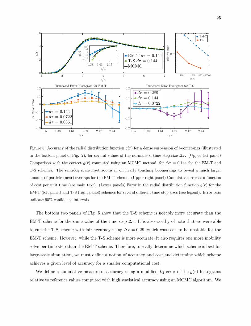
25

Figure 5: Accuracy of the radial distribution function g(r) for a dense suspension of boomerangs (illustrated

in the bottom panel of Fig. 2), for several values of the normalized time step size ∆τ . (Upper left panel)

Comparison with the correct g(r) computed using an MCMC method, for ∆τ = 0.144 for the EM-T and

T-S schemes. The semi-log scale inset zooms in on nearly touching boomerangs to reveal a much larger

amount of particle (near) overlaps for the EM-T scheme. (Upper right panel) Cumulative error as a function

of cost per unit time (see main text). (Lower panels) Error in the radial distribution function g(r) for the

EM-T (left panel) and T-S (right panel) schemes for several different time step sizes (see legend). Error bars

indicate 95% confidence intervals.

The bottom two panels of Fig. 5 show that the T-S scheme is notably more accurate than the

EM-T scheme for the same value of the time step ∆τ . It is also worthy of note that we were able

to run the T-S scheme with fair accuracy using ∆τ = 0.29, which was seen to be unstable for the

EM-T scheme. However, while the T-S scheme is more accurate, it also requires one more mobility

solve per time step than the EM-T scheme. Therefore, to really determine which scheme is best for

large-scale simulation, we must define a notion of accuracy and cost and determine which scheme

achieves a given level of accuracy for a smaller computational cost.

We define a cumulative measure of accuracy using a modified L2 error of the g(r) histograms

relative to reference values computed with high statistical accuracy using an MCMC algorithm. We

26

account for statistical errors by considering a weighted L2 norm proportional to the log-likelihood,

Error :=

√1

2

∫ R

0

(g∆t(r)− gMCMC(r)

σ(r)

)2

dr, (36)

where σ(r) is the standard deviation estimated empirically using multiple independently-seeded

simulations. We take R = 2.5a since for r & 2.5a the error in g(r) is dominated by sampling

(statistical) error for both schemes.

Since in our specific case the computational cost is dominated by (dense) multiplications of the

blob-blob mobility matrix with a vector, we define the cost per unit time as the (average) total

number of multiplications by M per time step, divided by ∆τ . We observe that when a solver

tolerance of 10−3 is used, the preconditioned iterative methods to solve the saddle point system,

and to compute M1/2, will both converge in 5 iterations most of the time. Thus, the total number

of multiplications per time step for the T-S scheme is 22 (3 × 5 + 5 + 2 for three mobility solves,

one Lanczos iteration, and one RFD on M), while the EM-T scheme requires 17 (2× 5 + 5 + 2).

The upper right panel of Fig. 5 shows that the T-S scheme costs less per unit time than the

EM-T scheme for any desired accuracy. We will therefore use the T-S schemes in Section IV C, and

recommend it for suspensions confined above a no-slip wall. Nevertheless, the cost of each scheme

depends heavily on how expensive it is to compute the action of M and M12 , and we recommend

repeating the cost-accuracy balance computations reported here for each specific application/code.

C. Uniform suspensions of Brownian Rollers

Active suspensions of rotating spherical colloids (microrollers) sedimented above a bottom wall

have been recently investigated using both experiments and simulations [4]. The colloids have an

embedded hematite which makes them weakly ferromagnetic and thus easily rotated by an external

magnetic field, as illustrated in Fig. (6). Because of the presence of a nonzero rotation-translation

coupling due to the bottom wall, micro-rollers translate parallel to the wall. Collective flow effects

dominate the dynamics of many-body suspensions, and the particles translate much faster at larger

densities. For non-uniform suspensions, shocks were observed to form and destabilize into fingering

instabilities, and deterministic simulations were performed to interrogate the observations. In [5],

the effects of Brownian motion were included in the simulations to demonstrate the quantitative

effect that fluctuations have on the the development and progression of the fingering instability. In

particular, it is important to note that Brownian motion sets the equilibrium gravitational height

of the colloids, and therefore must be included to obtain quantitative predictions that can directly

27

be compared to experiments. In [37], the nonlocal nature of the shock front was further elucidated,

and propagation of density waves in a uniform suspension translating parallel to the wall was

investigated using both experiments and simulation. One of the key parameters that enters in the

simplified equations describing the dynamics of density fluctuations (see Eq. (4) in [37]) around a

uniform state is the mean suspension velocity V .

Figure 6: A snapshot of a steadily-translating uniform suspension of 256 microrollers, each made up of 42

blobs (colored by their height above the floor), at planar packing density φ = 0.4. Each particle has an

embedded magnet, illustrated as a cluster of fuchsia blobs. Note that although for constant applied torque

the particle orientation does not enter in the equations of motion for translation, our algorithm keeps track

of the orientation of each colloid, which can be used to more accurately compute a time-dependent magnetic

torque on the particles if desired.

At higher densities, the mean velocity V is dominated by collective effects and near-field hydro-

dynamic interactions between the particles and between the particles and the wall. In all prior work

[5, 37], rollers were represented using only one blob, and the Rotne-Prager-Blake tensor was used to

add the active translation as a deterministic forcing term. In [10], it was demonstrated that using

more blobs to discretize spherical particles gives much greater accuracy for hydrodynamics. We are

here able to, for the first time, consistently and sufficiently accurately resolve hydrodynamics and

account for thermal fluctuations, and thus obtain quantitative predictions that can be compared

to experiments. Following [5], we take η = 1 mPa·s, the hydrodynamic radius of the particles

Rh = 0.656 µm, excess (buoyant) mass meg = 1.24 × 10−14 kg ms2

, and apply a constant, identical

torque on every particle, T = 8πηωR3hy, where we take the angular frequency ω = 10Hz. We use

28

the T-S scheme with ∆t = 0.008s. The particle-particle and particle-wall interaction potentials

are as described in [5]. We discretize the rollers using 1, 12, or 42 blobs (illustrated in Fig. (6)),

following [10]. It is important to note that for 12 or 42 blobs per particle the translation-rotation

coupling inducing the active motion is captured by the multiblob model itself rather than added by

hand as it is for a single blob. After an initial, transient period, we computed individual particle

velocities over intervals of 1/24s, and collected histograms of particles’ velocities at the steady

translating state [49]. Different time intervals to compute the velocity were also explored but no

substantial change was observed.

0 1 2 3 4 5 6

h/Rh

0

0.25

0.5

0.75

1

1.25

P(h)×R

h

Height Distribution, φ =0.2

1 blobs12 blobs42 blobsEquilibrium

0 5 10 15 20 25 30

V (µm/s)

0

0.05

0.1

0.15

P(V

)

Velocity Distribution, φ =0.2

0 2 4 6 8

h/Rh

0

0.25

0.5

0.75

1

1.25

P(h)×R

h

Height Distribution, φ =0.4

1 blobs12 blobs42 blobsEquilibrium

-10 0 10 20 30 40 50

V (µm/s)

0

0.05

0.1

P(V

)

Velocity Distribution, φ =0.4

-10-5 0 5 10 15 20 25 30 35 400

0.02

0.04

0.0642 blobsh/Rh < 2h/Rh > 2

-5 5 15 25 35 45 550

0.01

0.02

0.03

0.04 42 blobsh/Rh < 2h/Rh > 2

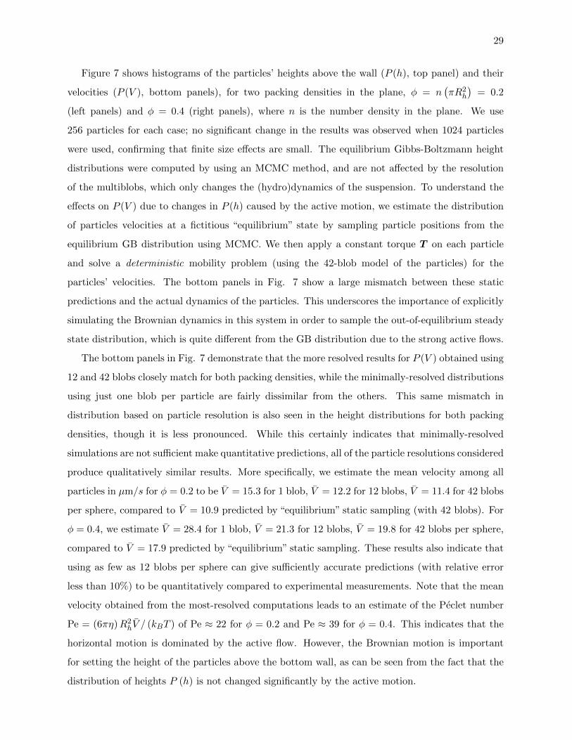
Figure 7: Histograms of the microrollers’ heights above the wall (P (h), top panels) and their velocities

(P (V ), bottom panels), for two packing densities in the plane, φ = 0.2 (left panels) and φ = 0.4 (right

panels), for a (pseudo)periodic active suspension at steady state. Solid vertical lines demarcate the mean of

the velocity distributions. Curves marked “equilibrium” use particle positions sampled from the equilibrium

GB distribution (in the absence of activity) using an MCMC method. All other curves are results of dynamic

BD simulations using the T-S scheme and either 1, 12 or 42 blobs to resolve each spherical colloid. (Top

panels) Comparison of the height distribution P (h) for φ = 0.2 (right) and φ = 0.4 (left), as set by a balance

of thermal noise, active vertical flows and gravity. (Bottom panels) Comparison of the velocity distribution

P (V ) for φ = 0.2 (right) and φ = 0.4 (left). For the curves marked as equilibrium, velocities were generated

by solving a deterministic mobility problem with particles discretized by 42 blobs, using configurations

sampled by an MCMC method. Insets show P (V ) for the finest resolution split into two groups based on

particle height (h ≶ 2Rh), where the normalization factor for the distributions is based on the fraction of

the total number of particles in the given subgroup.

29

Figure 7 shows histograms of the particles’ heights above the wall (P (h), top panel) and their

velocities (P (V ), bottom panels), for two packing densities in the plane, φ = n(πR2

h

)= 0.2

(left panels) and φ = 0.4 (right panels), where n is the number density in the plane. We use

256 particles for each case; no significant change in the results was observed when 1024 particles

were used, confirming that finite size effects are small. The equilibrium Gibbs-Boltzmann height

distributions were computed by using an MCMC method, and are not affected by the resolution

of the multiblobs, which only changes the (hydro)dynamics of the suspension. To understand the

effects on P (V ) due to changes in P (h) caused by the active motion, we estimate the distribution

of particles velocities at a fictitious “equilibrium” state by sampling particle positions from the

equilibrium GB distribution using MCMC. We then apply a constant torque T on each particle

and solve a deterministic mobility problem (using the 42-blob model of the particles) for the

particles’ velocities. The bottom panels in Fig. 7 show a large mismatch between these static

predictions and the actual dynamics of the particles. This underscores the importance of explicitly

simulating the Brownian dynamics in this system in order to sample the out-of-equilibrium steady

state distribution, which is quite different from the GB distribution due to the strong active flows.

The bottom panels in Fig. 7 demonstrate that the more resolved results for P (V ) obtained using

12 and 42 blobs closely match for both packing densities, while the minimally-resolved distributions

using just one blob per particle are fairly dissimilar from the others. This same mismatch in

distribution based on particle resolution is also seen in the height distributions for both packing

densities, though it is less pronounced. While this certainly indicates that minimally-resolved

simulations are not sufficient make quantitative predictions, all of the particle resolutions considered

produce qualitatively similar results. More specifically, we estimate the mean velocity among all

particles in µm/s for φ = 0.2 to be V = 15.3 for 1 blob, V = 12.2 for 12 blobs, V = 11.4 for 42 blobs

per sphere, compared to V = 10.9 predicted by “equilibrium” static sampling (with 42 blobs). For

φ = 0.4, we estimate V = 28.4 for 1 blob, V = 21.3 for 12 blobs, V = 19.8 for 42 blobs per sphere,

compared to V = 17.9 predicted by “equilibrium” static sampling. These results also indicate that

using as few as 12 blobs per sphere can give sufficiently accurate predictions (with relative error

less than 10%) to be quantitatively compared to experimental measurements. Note that the mean

velocity obtained from the most-resolved computations leads to an estimate of the Peclet number

Pe = (6πη)R2hV / (kBT ) of Pe ≈ 22 for φ = 0.2 and Pe ≈ 39 for φ = 0.4. This indicates that the

horizontal motion is dominated by the active flow. However, the Brownian motion is important

for setting the height of the particles above the bottom wall, as can be seen from the fact that the

distribution of heights P (h) is not changed significantly by the active motion.

30

All of the simulation results in Fig. 7 show bimodal distributions for both the particles’ heights

and velocities. Particularly prominent in the particle velocity distribution for φ = 0.4, but present

for φ = 0.2 as well, are two peaks indicating the existence of two distinct populations of “fast” and

“slow” particles. Close examination of the height distributions reveals a similar bimodality, and

our simulations indicate a strong correlation between particle height and velocity. We separate

particles into two subgroups roughly corresponding to the two peaks in P (h), and identify the fast

particles as the group corresponding to h > 2Rh, while the remaining particles are slower, as seen

in the inset figures in the lower panels of Fig. 7. This separation is surprising as we might expect

the opposite given that a single particle will translate faster if it is placed closer to the wall. This

indicates the importance of collective flows and packing effects in these suspensions. Physically,

the higher packing density causes a relatively dense monolayer of particles to form around the

gravitational height, hG = Rh + kBT/meg ≈ 1µm. The rest of the particles form a sparser and

more diffuse (in the vertical direction) monolayer above the first at height of roughly 2hG, and are

rapidly advected by the collective flow as they “slide” on top of the bottom layer.

The presence of two populations of particles at different heights and moving at different velocities

makes experimental measurements of P (V ) or even V more difficult. Namely, at these packing

densities it is not possible to track individual particles to measure individual particle velocities,

and indirect method such as particle image velocimetry (PIV) are used to estimate V , which can

lead to bias in the presence of fast and slow particles. Direct comparison of our computational

estimates to experimental measurements is therefore deferred for future work.

V. CONCLUSIONS

In this work we designed efficient and robust temporal integrators for the simulation of many

rigid particles suspended in a fluctuating viscous fluid. Hydrodynamic interactions were computed

using a rigid multiblob model [10] of the particles, and here we proposed a method to generate the

Brownian increments of the particles at a computational cost that is no larger than that of solving a

mobility problem. We demonstrated that the block-diagonal preconditioner used to solve mobility

problems in [10] is equally effective as a preconditioner for the Lanczos algorithm to compute

Brownian increments for the blobs. The stochastic drift term arising from the configuration-

dependent mobility matrix were computed using traction-corrected or slip-corrected random finite

differences. We presented a traction-corrected Euler-Maruyama scheme (EM-T) (algorithm 1),

as well as a slip-corrected Trapezoidal scheme (T-S) (algorithm 2). We have made our python

31

implementation (with PyCUDA acceleration) of the methods described here available at https:

//github.com/stochasticHydroTools/RigidMultiblobsWall. Both the EM-T and T-S schemes

scale linearly in complexity with the number of rigid particles being simulated if the iterative

methods used to compute deterministic and Brownian blob velocities are based on fast methods.

We confirmed that both schemes correctly reproduce the equilibrium Gibbs-Boltzmann distribution

for sufficiently small time step sizes, and found the T-S scheme to be notably superior in accuracy

for the same computational effort for large-scale problems. We used the T-S scheme to study the

non-equilibrium dynamics of an active suspension of microrollers confined above a no-slip bottom

wall, and demonstrated that as few as 12 blobs per sphere gives numerical errors on the order of

10% or less, unlike previous simulations of existing microroller experiments [5, 37]. The use of

particle image velocimetry (PIV) in [4] to experimentally estimate the average particle velocity

can be biased from the bimodality of the particle velocities, rendering a direct comparison with

experimental results currently unobtainable. In section IV C, we identified two well separated,

unimodal, populations of microrollers demarcated by their heights. This separation can perhaps

be used to design new experimental techniques to accurately measure the particles’ velocities within

each population.

There are number of application-dependent parameters that can be tweaked to improve effi-

ciency. For instance if small particle displacements are expected over a time step, one can wait

several time steps before recomputing the (Cholesky) factorizations of M that enter in the block-

diagonal preconditioner. Here we used the same relative error tolerance for all iterative methods,

and found a relatively loose tolerance of 10−3 to be sufficient. However, one could use a different

solver tolerances in, for example, steps 1,2, and 3 of algorithm 1 for the EM-T scheme. Further,

while the EM-T and T-S schemes were found to be optimal for the applications considered herein,

other schemes such as an Adams-Bashforth variant of the EM-T scheme, or a midpoint variant of

the T-S scheme are straightforward extensions and may prove optimal for other applications and

implementations. In fact, our biggest contribution here is the development of the traction-corrected

and slip-corrected RFDs, which can be used as tools to construct other schemes. It is important

to realize that showing theoretically that a certain scheme is consistent in the limit ∆t→ 0 is not

sufficient – establishing numerically that the scheme is robust for ∆t on the order of the diffusive

time scale, as we have done here for the EM-T and T-S schemes, is crucial. While we do not have a

detailed theoretical understanding of the errors that arise for finite ∆t, one important consideration

is that RFDs only give the stochastic drift term in expectation, and it is important to control and

reduce their variance and not just their mean.

32

The methods presented in this work are fairly general and can be extended to other geometries

and ways of computing hydrodynamic interactions. In periodic domains, we can use the Positively

Split Ewald (PSE) method [16] to compute deterministic and Brownian blob velocities, and no

change is made in algorithms 1 or 2 to account for this. However, in this case, generating Brownian

blob displacements becomes rather inexpensive compared to a mobility solve, and it is possible

that a midpoint split scheme would become preferable over the T-S scheme in terms of efficiency-

accuracy balance. Note that the PSE method could be extended to other geometries such as doubly-

periodic domains (e.g., membranes) by building on recently-developed Spectral Ewald methods

[41, 42]. To the best of our knowledge, there is presently no known method to compute Brownian

blob increments for infinite unbounded domains in (near) linear time; we relied here explicitly

on the the simplicity of the Rotne-Prager-Blake tensor and the screening by the wall to handle

particles confined in a half-space.

All of the computations performed in this work used a rather coarsely resolved multiblob model

to represent the rigid bodies. In future work, we will apply the temporal integrators proposed here

to more accurate representations of the geometry and hydrodynamics using the recently-developed

Fluctuating Boundary Integral Method (FBIM) [26]. Both of the temporal integrators presented

here can be used without modification with FBIM, but a midpoint scheme may be preferable

because of the low-cost of computing Brownian terms compared to solving mobility problems.

All of the methods presented herein relied extensively on an explicit representation of M,

which restricts the choice of domain and boundary conditions that we may use to those for which

an analytical expressions (and preferably a fast method to compute its action) for the RPY mobility

is available. In [24] the Stokes equations are solved explicitly on an Eulerian grid for fully confined

domains such as slit channels, and Immersed Boundary (IB) interpolation and spreading operators

are used to couple the blobs to the fluid solver. This Green’s-function-free or “explicit-solvent”

(but still inertia-less) approach implicitly computes the action of M in linear time in the number

of fluid grid cells. Some of us demonstrated in [24] that the action of M12 can also be computed

using the IB approach at minimal additional cost by using fluctuating hydrodynamics. In [10, 25],

the IB approach was extended to rigid bodies (multiblobs), but without accounting for Brownian

motion. The schemes presented herein can, in principle, be used with only minor modification with

the rigid-body IB method to simulate Brownian motion of rigid particles in fully confined domains,

when explicit representation of M is not available. However, the efficiency of the methods used in

this work hinged on the action of M being computed rapidly, and hence the temporal integrators

should be modified to account for the comparatively expensive explicit-solvent IB solvers introduced

33

in [10]. Efficient simulation of rigid, Brownian particles in general confined domains will be the

subject of future work.

Acknowledgments

We are grateful to Blaise Delmotte for his help with simulations of active roller suspensions, and

to Michelle Driscoll and Paul Chaikin for numerous discussions about experiments on microrollers.

This work was supported in part by the National Science Foundation under collaborative award

DMS-1418706 and by DMS–1418672, and by the U.S. Department of Energy Office of Science,

Office of Advanced Scientific Computing Research, Applied Mathematics program under award DE-

SC0008271. We thank the NVIDIA Academic Partnership program for providing GPU hardware

for performing the simulations reported here.

34

Appendix

Appendix A: EULER-MARUYAMA SCHEME

In section III we noted that a simple means of computing an RFD on B ≡ N , is to use

∆P = ∆Q =√kBTW in equation (17), where W is a vector drawn from the standard normal

distribution. However, incrementing the translational and rotational components of the configu-

ration Q by the same quantity may cause translation and rotation of a body by very different

magnitudes. This, in turn, may result in large variance of the quantity ∂QN :[WW T

](see (17)),

and hence slow the convergence to ∂Q ·N in expectation. To remedy this, we simply ensure that

a given body is being randomly translated and rotated by the same amount.

Specifically, we choose a length scale, Lp, to represent the size of body p, and compute the

random displacement,

∆Qp =

LpW fp

W τp

(A1)

as well as the random forces and torques,

W FTp = kBT

L−1p W

fp

W τp

(A2)

where W fp ,W

τp are both three dimensional standard Gaussian random vectors, and we form the

composite vectors W FT =[W FT

p

]and ∆Q =

[∆Qp

]. The drift can then be computed using a

simple RFD,

1

δ

⟨{N(Q+

δ

2∆Q

)−N

(Q− δ

2∆Q

)}W FT

⟩= kBT ∂Q ·N +O(δ2), (A3)

which respects the physical units of the problem and minimizes the variance of the approximation.

A one-sided difference approximation can be defined analogously.

Algorithm 3 summarizes a scalable implementation of the Euler-Maruyama RFD scheme from

[11] to solve (1), using a random finite difference similar to (A3) to compute the drift. Imple-

mentation of this scheme requires three solutions of the saddle point system (6) and one Lanczos

application per timestep.

Appendix B: PROOFS OF CONSISTENCY OF TEMPORAL INTEGRATORS

In this appendix we demonstrate that the two temporal integrators presented in this work

generate the required stochastic drift terms. In all of the calculations of this section, we will

35

Algorithm 3 Euler-Maruyama-RFD scheme

1. Compute RFD terms:

(a) Form W FT =[W FT

p

], where

W FTp = kBT

L−1p W

fp

W τp

.(b) Displace the particles by small random amounts:

Q±p = Qn

p ±δ

2

LpW fp

W τp

.(c) Solve two mobility problems for U+,U−: M± −K±

−(KT)±

0

λ±

U±

=

0

−W FT

.2. Compute

(M1/2

)nW n using a preconditioned Lancoz method or PSE.

3. Solve mobility problem: Mn −Kn

−(KT)n

0

λnUn

=

−√ 2kBT∆t

(M1/2

)nW n

−F n

.4. Update configuration:

Qn+1 = Qn + ∆t

{Un +

1

δ(U+ −U−)

}.

use index notation with the convention of summing over repeated indices. We will also use the

convention that superscripted indices correspond to a matrix inverse, i.e[A−1

]ij≡ Aij . To avoid

possible confusion with our superscript notation for the time level at which an operator is evaluated,

we will assume that all terms and operators are evaluated at the base configuration Q ≡ Qn unless

otherwise noted. We denote partial derivatives with the shorthand notation ∂k ≡ ∂/∂Qk.

1. Overdamped Langevin Equation using Quaternions

In principle, any means of representing orientation could be used with the techniques detailed in

this work. In previous work [11], unit quaternions were found to be a particularly favorable choice,

and we will use normalized quaternions to represent the orientation θ hereafter. Here we briefly

review key notation and results regarding quaternions; details can be found in [11]. A normalized

36

quaternion is a vector θ = [s,p] ∈ R4 such that ‖θ‖2 = 1. We define an orientation dependent

4× 3 “projection” matrix Ψ as

Ψ (θ) =1

2

−pTsI − P

, (B1)

where P is the cross product matrix defined by Px = p× x. For a configuration, Q = [q,θ] and

a rigid body velocity U = [u,ω], we introduce a matrix

Ξ =

I 0

0 Ψ

, (B2)

so that we may write dQ/dt = ΞU . In [11] some of us showed that the overdamped Langevin Ito

equation (1) may be written using unit quaternions as

dQl

dt= ΞliN ijF j + kBT (Ξli {∂kN ij}Ξkj + {∂kΞli}N ijΞkj) +

√2kBT ΞliN

1/2it W t (B3)

= Ξli ◦(N ijF j + kBT {∂kN ij}Ξkj +

√2kBT N 1/2

it W t

)= Ξli ◦U i,

where ◦ denotes the Stratonovich product. As shown in [11], the forces and torques of the system

may be written as F j = −Ξkj∂kU, where U (Q) is the conservative potential. This, combined with

the fact that ∂kΞkj = 0, allows us to recognize (B3) as having the same form as equation (1) but

with N replaced by ΞNΞT .

In order to discretize (B3), we write an expansion in ∆t for the procedure which rotates a

quaternion θ by an angular displacement ω∆t as

Rotate (θk,ωk∆t) ≈ θk + ∆tΨkjωj −∆t2

8‖ω‖22 θk. (B4)

The second order term in (B4) is responsible for the fact that that a simple (inconsistent) Euler-

Maruyama scheme without an RFD, using a velocity

U i = N ijF j +

√2kBT

∆tN 1/2

it Wnt (B5)

to update the configurations to the next time step, will generate the drift term

(kBT ) {∂kΞli}N ijΞkj in (B3) to leading order in ∆t [11]. This is to say that the rotate pro-

cedure (B4) naturally captures the Stratonovich product in the second line of (B3). A one-step

numerical scheme is first-order weakly accurate if the first three moments of the numerical update

are correct to O(∆t) [43]; the third moment in our schemes is easily seen to be at least O(∆t3/2).

37

Hence, to show that the schemes introduced in this work are weakly first order in solving (B3), we

will show that velocity used to update the configurations to the next time step is of the form

U i = N ijF j +

√2kBT

∆tN 1/2

it Wnt + kBT {∂kN ij}Ξkj +R

(∆t, ∆t1/2

), (B6)

where the notationR(a, b1/2

)denotes a Gaussian random error term with mean O (a), and variance

O (b). Notice that the leading order term in (B6), the Brownian velocity√

2kBT∆t N 1/2

it Wnt , controls

the second moment of the velocity update. This term is easily identified in the velocity update

produced by the schemes introduced in this work. The main difficulty is showing that both schemes

generate in expectation value the required drift term kBT {∂kN ij}Ξkj for sufficiently small ∆t.

For this, we will use the chain rule to expand the derivative,

∂kN ij =−N im

{∂kNml

}N lj = −N im (∂k {KpmMpqKql})N lj

=−N im {∂kKpm}MpqKqlN lj −N imKpm {∂kMpq}KqlN lj −N imKpmMpq {∂kKql}N lj

=−N im {∂kKsm}MsqKqlN lj (B7)

+ N imKpmMpr {∂kMrs}MsqKqlN lj

−N imKpmMpr {∂kKrl}N lj .

Note that the expression for (∂Q ·N )i can be obtained by replacing every instance of the index k

with j in the above. For clarity but without loss of generality, we take F = 0 hereafter. Note that

a nonzero value of F may affect the variance of a velocity update and thus the accuracy of the

scheme for finite values of ∆t. Still, the weak order of accuracy of the schemes considered will be

maintained for nonzero F .

2. Traction-Corrected Euler-Maruyama Scheme

It is immediate from the discussion in section II B, that the Brownian velocities produced by

Algorithm 1 are√

2kBT∆t N 1/2

ij Wnj to leading order in ∆t, and hence produce the correct second

moment. We will now show that the velocity produced in step 3 of Algorithm 1 is such that

〈Uni 〉 = kBT {∂kN ij}Ξkj +O

(δ2). (B8)

First, we may write step 3 as

Uni = −N imD

Fm + N imKpmMpr

(DSr +

√2kBT

∆tM1/2

rj Wnj

)

= −N imDFm + N imKpmMprDS

r +

√2kBT

∆tN 1/2

ij Wnj

38

and thus

〈Uni 〉 = −N im

⟨DFm

⟩+ N imKpmMpr

⟨DSr

⟩. (B9)

We can expand the quantities DFm and DS

r , defined in step 1d, using the definition of λRFD from

step 1b,

URFDl = N ljW

FTj

λRFDs = MsqKqlU

RFDl = MsqKqlN ljW

FTj .

Beginning with DFm,

⟨DFm

⟩=

1

δ

⟨{Ksm

(Q+)−Ksm

(Q−)}

MsqKqlN ljWFTj

⟩(B10)

= {∂kKsm}MsqKqlN lj

⟨∆Qk W

FTj

⟩+O(δ2). (B11)

Using the expansion for the rotation procedure from (B4), we may write ∆Qk = [∆qk,∆θk] as

∆qk =δ

2LpW

fk

∆θk =δ

2ΨklW

τl +R

(δ2, δ2

),

from which it is straightforward to verify that

⟨∆Qk W

FTj

⟩= kBT Ξkj +O(δ2). (B12)

Using equations (B11) and (B12), we see that the terms produced by DF give one part of the

required stochastic drift term,

⟨DFm

⟩= kBT {∂kKsm}MsqKqlN ljΞkj +O(δ2). (B13)

Now, for the contributions from terms involving DSr , we have

⟨DSr

⟩=

1

δ

⟨{Mrs

(Q+)−Mrs

(Q−)}

MsqKqlN ljWFTj

⟩− 1

δ

⟨{Krl

(Q+)−Krl

(Q−)}

N ljWFTj

⟩= ({∂kMrs}MsqKql − {∂kKrl})N lj

⟨∆Qk W

FTj

⟩+O(δ2), (B14)

and hence, using equations (B14) and (B12), we see that from DS we get two more pieces of the

required stochastic drift term,

⟨DSr

⟩= kBT ({∂kMrs}MsqKql − {∂kKrl})N ljΞkj +O(δ2). (B15)

39

Plugging the results from equations (B13) and (B15) into equation (B9), and using (B7), gives

〈Uni 〉 =−N im

⟨DFm

⟩+ N imKpmMpr

⟨DSr

⟩+O(δ2) (B16)

=− kBT (N im {∂kKsm}MsqKqlN ljΞkj

+ NKpmMpr {∂kMrs}MsqKqlN ljΞkj

−NKpmMpr {∂kKrl}N ljΞkj) +O(δ2)

=kBT {∂kN ij}Ξkj +O(δ2),

where the last equality comes directly from equation (B7). This is the desired result (B8).

3. Slip-Corrected Trapezoidal Scheme

We must show that the velocity used to update the position in the corrector step in Algorithm

2,

U(c)i =

1

2

(U i +Un

i

), (B17)

satisfies (B6) in law to leading order. We first show that the predictor-corrector update already

gives part of the required drift term. For this we set DF = DS = 0 (recall that we take F = 0 for

simplicity), and show that to leading order in ∆t, the velocity update in step 6 of Algorithm 2 is

such that [50] ⟨U

(c)i

⟩= −kBT N imKpmMpr {∂kKrl}N ljΞkj +O (∆t) . (B18)

To show this we first write steps 3 and 5 as

Unj =

√2kBT

∆tN jlKqlMqsM1/2

su W nu, (B19)

U i =

√2kBT

∆tN imKpmM

prM1/2

rt Wnt , (B20)

and write the velocity update of step 6 as√2∆t

kBTU

(c)i =N imKpmMprM1/2

rt Wnt + N imKpmM

prM1/2

rt Wnt

=N imKpmMprM1/2rt W

nt

+(N imKpmMpr + ∂k {N imKpmMpr} ∆Qk +O

(∆Q

2))

M1/2rt W

nt (B21)

=2N imKpmMprM1/2rt W

nt + ∂k {N imKpmMpr}M1/2

rt ∆QkWnt +R

(∆t3/2,∆t

)=2N 1/2

it Wnt + ∂k {N imKpmMpr}M1/2

rt ∆QkWnt +R

(∆t3/2,∆t

). (B22)

40

In equation (B21), we have used the fact that all operators with tilde are evaluated at Q, with

∆Q = Q−Qn.

All that remains is to compute,⟨U

(c)i

⟩=

√kBT

2∆t∂k {N imKpmMpr}M1/2

rt

⟨∆QkW

nt

⟩+O (∆t) . (B23)

Using the expansion for the rotate procedure (B4), we may write

∆Qk = ∆tΞkjUnj +R

(∆t2,∆t2

),

which combined with (B19) gives⟨∆QkW

nt

⟩=√

2∆tkBT ΞkjN jlKqlMqsM1/2su 〈W n

uWnt 〉+O(∆t2) (B24)

=√

2∆tkBT ΞkjN jlKqlMqsM1/2st +O(∆t2),

where we used 〈W nuW

nt 〉 = δtu. Hence, equation (B23) becomes,⟨

U(c)i

⟩=kBT ∂k {N imKpmMpr}M1/2

rt M1/2ts MsqKqlN ljΞkj +O (∆t) (B25)

=kBT ∂k {N imKpmMpr}MrsMsqKqlN ljΞkj +O (∆t)

=kBT ∂k {N imKpmMpr}KrlN ljΞkj +O (∆t)

where we used that MrsMsq = δrq. After expanding ∂k {N imKpmMpr} using the chain rule and

recalling that KpmMprKrl = Nml, we get⟨U

(c)i

⟩=kBT

({∂kN im}Ξkm (B26)

+ N im {∂kKpm}MprKrlN ljΞkj

+ N imKpm {∂kMpr}KrlN ljΞkj

)+O (∆t)

=− kBT N imKpmMpr {∂kKrl}N ljΞkj +O (∆t) . (B27)

where we have used (B7). This gives the desired result (B18).

We now include the contribution from nonzero DF and DS to show that U(c)i satisfies equation

(B6) as desired. Including the contributions from DF and DS , we may write the velocity update

of step 6 as,

U(c)i =− N imD

Fm + N imKpmM

prDSr

+

√kBT

2∆tN imKpmMprM1/2

rt Wnt +

√kBT

2∆tN imKpmM

prM1/2

rt Wnt . (B28)

41

Using equations (B22) and (B24), we may write this as

U(c)i =− N imD

Fm + N imKpmM

prDSr +

√2kBT

∆tN 1/2

it Wnt (B29)

+ ∂k {N imKpmMpr}M1/2rt

(ΞkjN jlKqlMqsM1/2

su WnuW

nt

)+R

(∆t,∆t1/2

).

In this form, it is easy to see that the scheme produces the correct Brownian velocity,√2kBT

∆t N 1/2it W

nt , and all that is left to verify is the first moment. Equation (B18) allows us

to immediately write the mean of (B29) as

⟨U

(c)i

⟩=⟨−N imD

Fm + N imKpmM

prDSr

⟩(B30)

− kBT N imKpmMpr {∂kKrl}N ljΞkj +O (∆t) .

We now examine the terms involving DFm and DS

r , separately. First, we note that using the

expanded rotate procedure (B4), steps 1c and 1b in algorithm 2 give

Q±k −Qk = ±δ Ξkj∆QRFDk +R

(δ2, δ2

)= ±δ ΞkjN jlKlqMqsW

Ds +R

(δ2, δ2

), (B31)

Using the definition of DFm from step 1d of Algorithm 2,

−N imDFm =− 1

δN im

{Kpm

(Q+)−Kpm

(Q−)}W

Fp

=− N im {∂kKpm} Ξkj∆QRFDk W

Fp +R

(δ2, δ2

)=−N im {∂kKpm} ΞkjN jlKlqMqsW

Ds W

Fp +R

(∆t,∆t1/2

)+R

(δ2, δ2

), (B32)

where we used (B31) in (B32). In expectation, we get the drift term⟨−N imD

Fm

⟩=−N im {∂kKpm}

⟨W

Ds W

Fp

⟩MsqKqlN ljΞkj +O

(δ2)

+O (∆t)

=− kBT N im {∂kKpm}MpqKqlN ljΞkj +O(δ2)

+O (∆t) , (B33)

where we have used that⟨W

Ds W

Fp

⟩= kBTδsp.

Similarly, using the definition of DSr from step 1d of Algorithm 2,

N imKpmMprDSr =

1

δN imKpmM

pr {Mrt

(Q+)−Mrt

(Q−)}W

Ft (B34)

=N imKpmMpr {∂kMrt} Ξkj∆QRFDk W

Ft +R

(∆t,∆t1/2

)+R

(δ2, δ2

).

Hence, taking the mean of (B34), gives⟨N imKpmM

prDSr

⟩=N imKpmMpr {∂kMrt}Ξkj

⟨∆QRFD

k WFt

⟩+O (∆t) +O(δ2)

=N imKpmMpr {∂kMrt}⟨W

Ds W

Ft

⟩MsqKqlN ljΞkj +O (∆t) +O(δ2)

=kBT N imKpmMpr {∂kMrs}MsqKqlN ljΞkj +O (∆t) +O(δ2). (B35)

42

Combining equations (B7), (B35) and (B33), we may write⟨−N imD

Fm + N imKpmM

prDSr

⟩= kBT ({∂kN ij}Ξkj + N imKpmMpr {∂kKrl}N ljΞkj)

+O (∆t) +O(δ2). (B36)

Combining this with (B30) and using equation (B7) gives the desired result (B6).

[1] R. M. Jendrejack, J. J. de Pablo, and M. D. Graham. Stochastic simulations of DNA in flow: Dynamics

and the effects of hydrodynamic interactions. J. Chem. Phys., 116(17):7752–7759, 2002.

[2] W. B. Russel. Brownian Motion of Small Particles Suspended in Liquids. Ann. Rev. Fluid Mech.,

13:425–455, 1981.

[3] Raymond Kapral. Perspective: Nanomotors without moving parts that propel themselves in solution.

J. Chem. Phys., 138:020901, 2013.

[4] Michelle Driscoll, Blaise Delmotte, Mena Youssef, Stefano Sacanna, Aleksandar Donev, and Paul

Chaikin. Unstable fronts and motile structures formed by microrollers. Nature Physics, 13:375–379,

2017.

[5] Florencio Balboa Usabiaga, Blaise Delmotte, and Aleksandar Donev. Brownian dynamics of confined

suspensions of active microrollers. J. Chem. Phys., 146(13):134104, 2017. Software available at https:

//github.com/stochasticHydroTools/RigidMultiblobsWall.

[6] Adolfo J Banchio and John F Brady. Accelerated stokesian dynamics: Brownian motion. The Journal

of chemical physics, 118:10323, 2003.

[7] Blaise Delmotte and Eric E Keaveny. Simulating brownian suspensions with fluctuating hydrodynamics.

The Journal of chemical physics, 143(24):244109, 2015.

[8] Rajesh Singh and R Adhikari. Fluctuating hydrodynamics and the brownian motion of an active colloid

near a wall. European Journal of Computational Mechanics, pages 1–20, 2017.

[9] Brendan D Hoffman and Eric SG Shaqfeh. The effect of brownian motion on the stability of sedimenting

suspensions of polarizable rods in an electric field. Journal of Fluid Mechanics, 624:361–388, 2009.

[10] F. Balboa Usabiaga, B. Kallemov, B. Delmotte, A. P. S. Bhalla, B. E. Griffith, and A. Donev. Hydro-

dynamics of suspensions of passive and active rigid particles: a rigid multiblob approach. Communica-

tions in Applied Mathematics and Computational Science, 11(2):217–296, 2016. Software available at

https://github.com/stochasticHydroTools/RigidMultiblobsWall.

[11] S. Delong, F. Balboa Usabiaga, and A. Donev. Brownian dynamics of confined rigid bodies. J. Chem.

Phys., 143(14):144107, 2015. Software available at https://github.com/stochasticHydroTools/

RigidMultiblobsWall.

[12] Constantine Pozrikidis. Boundary integral and singularity methods for linearized viscous flow. Cam-

bridge University Press, 1992.

43

[13] Ludvig Af Klinteberg and Anna-Karin Tornberg. Fast ewald summation for stokesian particle suspen-

sions. International Journal for Numerical Methods in Fluids, 76(10):669–698, 2014.

[14] Ludvig af Klinteberg and Anna-Karin Tornberg. A fast integral equation method for solid particles in

viscous flow using quadrature by expansion. Journal of Computational Physics, 326:420–445, 2016.

[15] Edmond Chow and Yousef Saad. Preconditioned krylov subspace methods for sampling multivariate

gaussian distributions. SIAM Journal on Scientific Computing, 36(2):A588–A608, 2014.

[16] A. M. Fiore, F. Balboa Usabiaga, A. Donev, and J. W. Swan. Rapid sampling of stochastic displace-

ments in brownian dynamics simulations. J. Chem. Phys., 146(12):124116, 2017. Software available at

https://github.com/stochasticHydroTools/PSE.

[17] M. Hutter and H.C. Ottinger. Fluctuation-dissipation theorem, kinetic stochastic integral and efficient

simulations. J. Chem. Soc., Faraday Trans., 94(10):1403–1405, 1998.

[18] James W Swan, John F Brady, Rachel S Moore, et al. Modeling hydrodynamic self-propulsion with

Stokesian Dynamics. Or teaching Stokesian Dynamics to swim. Physics of Fluids, 23:071901, 2011.

[19] Rajesh Singh, Somdeb Ghose, and R Adhikari. Many-body microhydrodynamics of colloidal particles

with active boundary layers. Journal of Statistical Mechanics: Theory and Experiment, 2015(6):P06017,

2015.

[20] Jens Rotne and Stephen Prager. Variational treatment of hydrodynamic interaction in polymers. The

Journal of Chemical Physics, 50:4831, 1969.

[21] Eligiusz Wajnryb, Krzysztof A Mizerski, Pawel J Zuk, and Piotr Szymczak. Generalization of the

rotne–prager–yamakawa mobility and shear disturbance tensors. Journal of Fluid Mechanics, 731:R3,

2013.

[22] Zhi Liang, Zydrunas Gimbutas, Leslie Greengard, Jingfang Huang, and Shidong Jiang. A fast multipole

method for the rotne–prager–yamakawa tensor and its applications. Journal of Computational Physics,

234:133–139, 2013.

[23] James W. Swan and John F. Brady. Simulation of hydrodynamically interacting particles near a no-slip

boundary. Physics of Fluids, 19(11):113306, 2007.

[24] S. Delong, F. Balboa Usabiaga, R. Delgado-Buscalioni, B. E. Griffith, and A. Donev. Brownian

Dynamics without Green’s Functions. J. Chem. Phys., 140(13):134110, 2014. Software available at

https://github.com/stochasticHydroTools/FIB.

[25] B. Kallemov, A. Pal Singh Bhalla, B. E. Griffith, and A. Donev. An immersed boundary method for

rigid bodies. Communications in Applied Mathematics and Computational Science, 11(1):79–141, 2016.

Software available at https://github.com/stochasticHydroTools/RigidBodyIB.

[26] Y. Bao, M. Rachh, E. Keaveny, L. Greengard, and A. Donev. A fluctuating boundary integral method

for Brownian suspensions. Submitted to J. Comp. Phys., preprint ArXiv:1709.01480, 2017.

[27] Z. Gimbutas, L. Greengard, and S. Veerapaneni. Simple and efficient representations for the fundamen-

tal solutions of Stokes flow in a half-space. Journal of Fluid Mechanics, 776:R1, 2015. Code available

at http://www.cims.nyu.edu/cmcl/fmm3dlib/fmm3dlib.html.

44

[28] David Saintillan, Eric Darve, and Eric SG Shaqfeh. A smooth particle-mesh ewald algorithm for stokes

suspension simulations: The sedimentation of fibers. Physics of Fluids, 17(3):033301, 2005.

[29] Mu Wang and John F Brady. Spectral ewald acceleration of stokesian dynamics for polydisperse

suspensions. Journal of Computational Physics, 306:443–477, 2016.

[30] Eric E. Keaveny. Fluctuating force-coupling method for simulations of colloidal suspensions. J. Comp.

Phys., 269(0):61 – 79, 2014.

[31] James W Swan and Gang Wang. Rapid calculation of hydrodynamic and transport properties in

concentrated solutions of colloidal particles and macromolecules. Physics of Fluids (1994-present),

28(1):011902, 2016.

[32] M. Fixman. Simulation of polymer dynamics. I. General theory. J. Chem. Phys., 69:1527, 1978.

[33] S. Delong, Y. Sun, B. E. Griffith, E. Vanden-Eijnden, and A. Donev. Multiscale temporal integrators

for fluctuating hydrodynamics. Phys. Rev. E, 90:063312, 2014. Software available at https://github.

com/stochasticHydroTools/MixingIBAMR.

[34] Andrew M Fiore and James W Swan. Rapid sampling of stochastic displacements in brownian dynamics

simulations with stresslet constraints. arXiv preprint arXiv:1709.06946, 2017.

[35] S. Delong, B. E. Griffith, E. Vanden-Eijnden, and A. Donev. Temporal Integrators for Fluctuating

Hydrodynamics. Phys. Rev. E, 87(3):033302, 2013.

[36] Ayan Chakrabarty, Andrew Konya, Feng Wang, Jonathan V Selinger, Kai Sun, and Qi-Huo Wei.

Brownian motion of boomerang colloidal particles. Physical review letters, 111(16):160603, 2013.

[37] Blaise Delmotte, Michelle Driscoll, Paul Chaikin, and Aleksandar Donev. Hydrodynamic shocks in

microroller suspensions. Phys. Rev. Fluids, 2:092301, 2017.

[38] Ayan Chakrabarty, Andrew Konya, Feng Wang, Jonathan V. Selinger, Kai Sun, and Qi-Huo Wei.

Brownian motion of arbitrarily shaped particles in two dimensions. Langmuir, 30(46):13844–13853,

2014.

[39] D. Frenkel and B. Smit. Understanding Molecular Simulation. Academic Press, 2002.

[40] Hoang-Ngan Nguyen and Karin Leiderman. Computation of the singular and regularized image systems

for doubly-periodic stokes flow in the presence of a wall. Journal of Computational Physics, 297:442–461,

2015.

[41] Dag Lindbo and Anna-Karin Tornberg. Fast and spectrally accurate summation of 2-periodic stokes

potentials. arXiv preprint arXiv:1111.1815, 2011.

[42] Oana Marin, Katarina Gustavsson, and Anna-Karin Tornberg. A highly accurate boundary treatment

for confined stokes flow. Computers & Fluids, 66:215–230, 2012.

[43] G.N. Milstein and M.V. Tretyakov. Stochastic numerics for mathematical physics. Springer, 2004.

[44] As explained in detail in Appendix A of [10], the rigid multiblob method can be seen as a first-kind

boundary integral method regularized in a physically-consistent way so as to ensure the symmetry and

positive definiteness of the mobility matrix, as required for adding Brownian motion.

[45] The random slip velocity u can be derived by using fluctuating hydrodynamics. For example, one can

45

start with the coupled fluid+particle equations given in Eq. (20) in [10], and then add a stochastic

stress tensor to the Stokes equation for the fluid velocity [24, 26]. After elimination of the fluid one

obtains (9). This can most simply be done by starting from the fully discrete saddle-point system (25)

in [10], adding the stochastic stress tensor as done in [24], and the using standard Schur complement

techniques to eliminate the fluid velocity and pressure.

[46] In this paper, we evaluate the action of M directly using a summation on the GPU, which gives

accuracy comparable to roundoff. But other more scalable implementations of the action of the RPY

mobility would use approximate methods like the fast multipole method (FMM) [22, 27] or the Spectral

Ewald method [16], which would have an input relative error tolerance of their own, larger than the

roundoff error.

[47] On many GPUs it is more efficient to use single-precision arithmetic.

[48] The midpoint slip scheme was much more robust than the midpoint traction scheme for larger ∆t.

[49] Note that the analysis in [37] shows that the steady uniform translating state is stable, and that density

fluctuations propagate as waves without growing or shrinking in time.

[50] Note that this quantity gives the drift term produced by equation (26) in section III B.