Broadband Pumping Effects on the Diode Pumped Alkali Laser
96
Air Force Institute of Technology AFIT Scholar eses and Dissertations Student Graduate Works 3-11-2011 Broadband Pumping Effects on the Diode Pumped Alkali Laser Paul Nathaniel Jones Follow this and additional works at: hps://scholar.afit.edu/etd Part of the Physics Commons is esis is brought to you for free and open access by the Student Graduate Works at AFIT Scholar. It has been accepted for inclusion in eses and Dissertations by an authorized administrator of AFIT Scholar. For more information, please contact richard.mansfield@afit.edu. Recommended Citation Jones, Paul Nathaniel, "Broadband Pumping Effects on the Diode Pumped Alkali Laser" (2011). eses and Dissertations. 1459. hps://scholar.afit.edu/etd/1459
Transcript of Broadband Pumping Effects on the Diode Pumped Alkali Laser

Air Force Institute of TechnologyAFIT Scholar
Theses and Dissertations Student Graduate Works
3-11-2011
Broadband Pumping Effects on the Diode PumpedAlkali LaserPaul Nathaniel Jones
Follow this and additional works at: https://scholar.afit.edu/etd
Part of the Physics Commons
This Thesis is brought to you for free and open access by the Student Graduate Works at AFIT Scholar. It has been accepted for inclusion in Theses andDissertations by an authorized administrator of AFIT Scholar. For more information, please contact [email protected].
Recommended CitationJones, Paul Nathaniel, "Broadband Pumping Effects on the Diode Pumped Alkali Laser" (2011). Theses and Dissertations. 1459.https://scholar.afit.edu/etd/1459

BROADBAND PUMPING EFFECTS ON THE DIODE PUMPED ALKALI LASER
THESIS
Paul Nathaniel Jones, Civilian
AFIT/GAP/ENP/11-M04
DEPARTMENT OF THE AIR FORCE AIR UNIVERSITY
AIR FORCE INSTITUTE OF TECHNOLOGY
Wright-Patterson Air Force Base, Ohio
APPROVED FOR PUBLIC RELEASE; DISTRIBUTION IS UNLIMITED

The views expressed in this thesis are those of the author and do not reflect the official policy or position of the United States Air Force. The Department of Defense, or the United States Government. This material is declared the work of the U.S. Government and is not subject to copyright protection in the United States.

AFIT/GAP/ENP/11-M04
BROADBAND PUMPING EFFECTS ON THE DIODE PUMPED ALKALI LASER
THESIS
Presented to the Faculty
Department of Engineering Physics
Graduate School of Engineering and Management
Air Force Institute of Technology
Air University
Air Education and Training Command
In Partial Fulfillment of the Requirements for the
Degree of Master of Science in Applied Physics
Paul Nathaniel Jones, BS Staff Scientist, AFIT
March 2011
APPROVED FOR PUBLIC RELEASE; DISTRIBUTION UNLIMITED.

AFIT/GAP/ENP/11-M04
BROADBAND PUMPING EFFECTS ON THE DIODE PUMPED ALKALI LASER
Paul Nathaniel Jones, B.S. Civilian
Approved: ______//signed//_____________ _______________ Glen P. Perram, PhD (Chairman) Date ______//signed//__________________ __________________ Lt. Col Jeremy C. Holtgrave (Member) Date __ ___//signed//______ _ ____ __________________ Maj. Clifford Sulham (Member) Date
iv
AFIT/GAP/ENP/11-M04
Abstract
This research seeks to gain greater insight on the mechanics of The Diode Pumped
Alkali Laser through analytic modeling techniques. This work is an extension to a
previous model developed by Dr. Gordon Hager, and focuses on the addition of pump-
beam bandwidth. Specifically, it seeks to determine the effect that broadband pumping
has on laser performance. The model incorporates all the fundamental parameters within
the laser system, including alkali concentrations, collision partner concentrations, pump
bandwidth, length and temperature of gain medium, transmission, and reflectivity.
Baseline operating conditions set Rubidium (Rb) concentrations ranging from 1012 - 1014
atoms/cm3, corresponding to operating temperatures ranging from 50 – 150 C. Ethane or
Methane concentrations are varied corresponding to partial pressures from 100 – 500
Torr. The system is evaluated for incident beam intensity ranging from 0 – 30000
W/cm2, for both lasing and non-lasing system analysis. Output laser beam intensities
scale well with input beam intensity and the model predicts optical to optical efficiencies
of over 70%.

v
AFIT/GAP/ENP/11-M04
To The Air Force Institute of Technology

vi
Acknowledgments
This work is the culmination of the efforts made by the faculty and staff of The Air
Force Institute of Technology. Of greatest influence was my mentor, Dr. Glen Perram.
His expertise, guidance, and patience created an environment where ideas were sparked,
obstacles were overcome, and progress was made. Second I would like to thank Greg
Smith and Michael Ranft. Their technical expertise and willingness to help enabled me
to make timely progress on my experiments. Finally, I would like to thank three of my
fellow graduate students, Greg Pitz, Cliff Sulham, and Matt Lange. Greg and Matt
welcomed me into AFIT in a very professional and helpful way and made my transition
into graduate school a success. Cliff was a true co-worker to me, and was someone I
could bounce ideas off of, get advice on experiments, and rely on for the many small
favors we experimenters ask of each other. Thank you.
Paul N. Jones
vii
Table of Contents
Page
Abstract……………………………………………………………………………….…..iv
Acknowledgements……………………………………………………….…………...…..v
List of Figures…………………………………………………………….……………..viii
List of Tables………………………………………………………………………….….xi
List of Symbols…………………………………………………………………….......….x
I. Introduction…………………………………………………………………………….1 Background…………………………………………………………………………….1 The Diode Pumped Alkali Laser.....................................................................................2 Analytic Modeling……………………………………………………………………..4 II. Literature Review……………………………………………………………………...6 Alkali Earth Metals……………………………………………….…………………....6 Diode Pumped Alkali Laser Technology………………………….………………….16 III. Methodology……………………………………………………………………...…21 Introduction…………………………………………………………………………...21 Longitudinally Averaged Two-Way Intra-Cavity Pump Beam Intensity………….…24 Laser Rate Equations…………………………………………………………………26 Transcendental Solution………………………………………………………………27 Frequency Dependence of the Pump Transition…………………………………...…29 IV. Results and Analysis………………………………………………………………...33 Introduction…………………………………………………………………………...33 Single Frequency, No Lasing Results………………………………………………...34 Single Frequency, Lasing Mode Results……………………………………………..35 Broadband Pump, Lasing Mode Results…………………………………………...…41 V. Conclusions and Discussion…...……………………………………………………..55 Appendix A. Rubidium Spectroscopic Data……………………………………………..59 Appendix B. Mathematica Code ……….…………………..…………………………...60 Bibliography……………………………………………………………………………..80

viii
List of Figures
Figure Page
1. DPAL Three Level Diagram (Rb)...……………………….……….………………..3
2. Rb D2 Hyperfine Structure…………………………………..……………………….9
3. Initial Population Inversion vs. Alkali Temperature………………………………..12
4. Rb Vapor Pressure vs. Temperature………………………………………………..14
5. Atmospheric Transmittivity………………………………………………………...15
6. Standard DPAL configuration……………………………………………………...18
7. Copper Waveguide Model and Results……………………………………………..19
8. Model Dependent Variables………………………………………………………..22
9. Round Trip Pump Beam Intensity………………………………………………….24
10. Transcendental Intersection……………………………………………………...…28
11. Ω vs Ipin……………………………………………………………….…………….29
12. D1 Spectral Overlap………………………………………………………………...30
13. Steady State Alkali Concentrations – Pre lasing………………………………...….34
14. Pre-Lasing Intracavity Pump Beam Intensity – Frequency Independent……….….35
15. Intracavity Laser Intensity – Frequency Independent……………..………………..36
16. Intracavity Pump Intensity – Frequency Independent……………………………...37
17. Ethane Variation – Frequency Independent…………………………………...……38
18. Rubidium Variation – Frequency Independent………………..……………………39
19. Transmittivity Variation – Frequency Independent………………………………...40
20. Cell Length Variation – Frequency Independent…………………………………..41
21. Ω vs Ipin – Frequency Dependent……………………...…………………………...42

ix
Figure Page
22. Ilase vs Ipin – Frequency Dependent………...………………………………………44
23. Ethane Variation – Frequency Dependent (19.73 GHz)………………..……….…44
24. Ethane Variation – Frequency Dependent (200 GHz)……………...…………...…44
25. Reflectivity Variation – Frequency Dependent……………………..……………..45
26. Δ -Bandwidth Variation – Frequency Dependent…………………………………46
27. Reflectivity Variation 3D – Frequency Dependent………………...………...……47
28. DPAL Efficiency – Frequency Dependent……………………………………...…48
29. Reflectivity Variation 2D – Frequency Dependent………….…………………….49
30. DPAL Efficiency – Frequency Dependent……………………………………..….50
31. Gamma – 300 Torr Ethane…………………………………………………………51
32. Gamma – 500 Torr Ethane…………………………………………………………51
33. Ω vs Ipin 500 Torr Ethane (500 Ghz)……………………………………………….51
34. Ilase vs. Log[Rb] – 500 Torr Ethane………………………………………………..52
35. Δ – 300 Torr Ethane………………………………………………………….……53
36. Grotrain Diagram – Laser Pumped Rb Fluorescence………………………….…..57

x
List of Tables
Table Page
1. Rb Spectroscopic Data…………………………………………………………………6
2. Alkali Quantum Efficiencies………………………………………………………...…8
3. Model Variable Definitions (Rb DPAL)………………………………………...……23
4. Baseline Parameters – Frequency Independent Case…………………………………33

xi
List of Symbols
Symbol Definition
………………………………………….………………….....…Einstein A-coefficient
c ………………………………..…………………………..… speed of light (in vaccuum)
Cs…………………………………………………………………………………...Cesium
E……………………………………………..………………………..ethane concentration
Fr…………………………………………………………………….……………Francium
gi…….…………………………………………………………………degeneracy of ith state
gth ………………………………..…………………………………….…… threshold gain
H…………………………………………………………………………………Hydrogen
h ………………………..………………………………….…………… Planck’s Constant
He ………………………………..………………………………… Helium concentration
Ipin………………………………………..………………………..Incident Pump Intensity
K……………………………………….……..………………………………….Potassium
k32………………………………..…..…………… spin-orbit mixing rate (ethane partner)
k ………………………………….……………………..…………… Boltzmann Constant
Li…………………………………………………………………………………...Lithium
lg …………………………………………..……………………………… gain cell length
Na………………………………………………………………………………..…Sodium
Ni……………………………………………………………population density of ith level
…………...………………….……………………………….….….quantum efficiency
r ………………………………..…………………………………… net cavity reflectivity

xii
Symbol Definition
Rb………………………………………………………………………….……..Rubidium
T ………………………………..……………………...…………… gain cell temperature
t21………………………………..……….………… radiative lifetime of upper laser level
t31………………………………..………………… radiative lifetime of upper pump level
ν21………………………..…………………………………… frequency of the laser beam
ν31………………………………..…………………..……… frequency of the pump beam
λ………………………..…………..………...…………... ………….…...……wavelength
π ………………………………………………………………….…………..…3.1415926
ΔE……………………………………………………………….…..… energy differential
σ21………………………………..……… absorption cross section on the lasing transition
σ31………………………..……………… absorption cross section on the pump transition
Ω ……………….…… longitudinally averaged two-way intracavity pump beam intensity
Ψ ………………….………………………… intracavity average two-way laser intensity
t …………………….…………..…………………………….…… net cavity transmission
Δν31………………………………………………..……………… pump beam bandwidth

1
BROADBAND PUMPING EFFECTS ON THE DIODE PUMPED ALKALI LASER
I. Introduction
Background
For decades the United States Military has been researching and developing high
energy lasers (HEL) for improved tactical advantages and anti-ballistic missile defense.
These weapons offer numerous advantages over conventional systems, and as Secretary
of the Air Force Widnall recognized in 1997: “It isn’t very often an innovation comes
along that revolutionizes our operational concepts, tactics and strategies. You can
probably name them on one hand – the atomic bomb, the satellite, the jet engine, stealth,
and the microchip. It’s possible the airborne laser is in this league.” With pinpoint
accuracy, HEL are capable of reducing collateral damage while achieving target
destruction. Their light speed trajectory enables them to engage targets immediately after
detection from a relatively safe distance. And finally, they are inexpensive to operate and
can be tailored for other purposes, including non-lethal destruction, and disruption [8].
The currently mounted HEL on the Airborne Laser (ABL) has proven effective yet
possesses a few undesirable characteristics. In February 2010, The ABL flew over the
coast of California and successfully targeted, tracked, and destroyed a ballistic missile in
its boost phase. This historical feat marks a breakthrough in operational status and
revolutionizes warfare. In fact, the Missile Defense Agency officially recognized this

2
fact by awarding its Technology Pioneer Award to three Boeing Airborne Laser Testbed
engineers and three of their government and industry teammates. Yet while this
achievement is groundbreaking and a warfare game-changer, criticism over the installed
systems logistical feasibility, size, and ammunitions reservoir is justified. This system is
a chemically driven laser which utilizes vast quantities of hazardous chemicals including
chlorine, iodine, hydrogen peroxide and potassium hydroxide, none of which are ideal for
storage in a war zone. After exhausting its 6-10 shot magazine depth, it would take two
C-17 transport planes to refuel, and due to atmospheric turbulence the ABL has a limited
range of approximately 600 km for liquid fueled ICBM and 300 km for solid fueled
ICBM. In addition, it takes the entire hull of a Boeing 747 to create weapons grade
power. However, it is still the only system capable of such high power on target. With
these factors in mind a pursuit for a lightweight, compact, low hazard risk, and high
magazine depth system has been underway.
The Diode Pumped Alkali Laser
According to experts in the field, the system which holds the most promise for
achieving these standards is the Diode Pumped Alkali Laser (DPAL). It was first
demonstrated in the early 90’s and patented by Krupke in 2003 [5]. These systems
utilize the cost and energy-effectiveness of diode bars, the thermal management
advantages of gas phase lasers, the simplicity of alkali earth metals, and are essentially an
efficient narrow-banding, laser photon engine [2].
An alkali, typically Rubidium (Rb) or Cesium (Cs), is heated to its gas phase and
subject to diode-driven laser light in resonance with its second lowest excited state (2P3/2).
A spin-orbit relaxer induces a rapid Boltzmann Equilibrium between the upper pump

3
state to the upper lasing state, or the lowest lying excited state (2P1/2). Spontaneous
emission from the 2P1/2 state to ground induces amplified stimulated emission leading up
to lasing. The energy level diagram below shows the optical-atomic and kinetic
processes involved.
The DPAL mass produces single mode, narrow-banded, near infrared (IR) laser
photons in a cyclic, three step process. As shown above, broadband, multimode diode
laser light centered at the D2 transition is incident on a vaporized alkali and buffer gas
mixture. This light excites the alkali into its second excited state. With the proper buffer
gas to alkali concentrations, rapid Boltzmann Equilibrium occurs through collision
Figure 1. DPAL Three Level Diagram (Rb)

4
processes causing relaxation from the upper 2P3/2, to the lower 2P1/2 state [2]. While the
energy split between the upper pump and upper lasing level is less than 1% of the pump
energy, at projected operating temperatures this equilibrium still places over 45% of the
alkali atoms in the upper lasing state, resulting in a high population inversion. Once the
alkali is in this state, (the upper lasing level), it slowly (with a radiative lifetime of 27.7
ns [5]), yet eventually begins to fluoresce back to ground. This causes those slowly
trickling spontaneous emission photons to see an inverted landscape upon release. Once
ejected, they pass through the gain medium and by stimulated emission “grab” photons
from other excited D1 atoms. As they grab these photons the projecting wave gains in
amplitude through amplified spontaneous emission (ASE) until reaching the end of the
gain cell.
Given a laser cavity and an emission trajectory within a mode of the respective
cavity, and assuming our gain exceeds threshold, this amplified wave will oscillate back
and forth through the gain medium exponentially increasing in amplitude after each pass.
Eventually and after multiple passes, the stimulated emission rate caused by the high
intensity oscillating laser beam overcomes the pump and spin-orbit relaxer rates, leading
to a saturated D1 to ground transition and the maximum intra-cavity laser intensity [2].
Analytical Modeling
In order to accurately model these events and predict the output beam strength of the
DPAL, a robust and quasi-analytic model has been developed by Dr. Gordon Hager [2].
This model accounts for all the substantial interactions and effects associated with DPAL
operation, including input beam intensity, alkali concentration, buffer gas concentration,
mirror reflectivity, cavity transmitivity and gain medium length. It integrates

5
fundamental laser physics with experimental results specific to the DPAL to produce
feasible and accurate results.
It has been advanced in order to take into effect the frequency dependence of the
pump beams interaction with the system. It creates an alkali cross-section bandwidth
function that is dependent on temperature and pressure, and also adds a frequency
dependence to the pump beam intensity. It shows that a close spectral overlap between
these two functions is paramount for optimal efficiency. Finally, it is also a beneficial
tool for analysis of gain medium kinetics, parametric studies, and helps to improve the
overall intuition of the staff, in hopes that a more clear and fundamental understanding
will lead to an efficient, powerful, and precisely controlled system.

6
II. Literature Review
In this chapter, a review of literature pertaining to the physics involved with the
DPAL is summarized. Also summarized is a review of publications on advancing DPAL
technology and a few small references to laser engineering. After establishing the
theoretical foundations of the DPAL and its current state of affairs an introduction to the
analytic model is made in the following chapter by a review of two of its author’s
publications.
Alkali Earth Metals
Alkali earth metals (alkalis) have been extensively researched and are an ideal
candidate for an optically pumped gain medium. First, they consist of the elements
possessing a single valence electron, making their electron energy levels relatively easy
to assign and well documented. The National Institute of Science and Technology has
publicized a table consisting of the more significant spectroscopic constants for each
element, and an excerpt from the table for Rb is shown below:
Table 1. Rb Spectroscopic Data [5]

7
A tabulation of each electronic transition in Rb corresponding to photonic
wavelengths from 740-880 nm along with the key spectroscopic constants of Einstein A
coefficients (column 2), initial and final electronic configurations (column 3), and the
degeneracy’s of the initial and final states (column 5). Key transitions in the DPAL (D1
at 795 nm and D2 at 780 nm) have well known wavelengths, Einstein A-coefficients ,
degeneracy ratios, and spin states. For a more complete listing of data for Rb see
Appendix A. The absorption cross-section is dependent on the Einstein A-coefficient and
is given by:
(1)
Where g2 is the degeneracy of the upper transition state and g1 of the lower. is the
Einstein A coefficient, is the transition wavelength, and is the normalized, unitless,
lineshape function (typically a Gaussian, Lorentzian, or Voigt profile). It is apparent that
absorption cross-sections scale linearly with Einstein A coefficients and it should also be
noted that alkalis possess some of the largest coefficients currently known, at linecenter
the D1 transition absorption cross-section has a published value of 4.92x10⁻¹³ cm2 [2,5].
Given such high cross-sections, alkalis are easily and efficiently energized through a
radiant source, or in the case of the DPAL, through diode laser pumping.
Another characteristic amongst the alkalis that proves them an effective laser gain
medium is their extremely high quantum efficiency (QE). In a laser, QE refers to the
ratio between the excitation transition and the lasing transition. Mathematically stated:
(2)

8
Where is the QE, and , are the pump and laser transition energies
respectively. It is the upper limit for the performance of any laser. It cannot be designed
and is solely dependent on energy levels of the gain medium. However, lasers can be
designed around QE, and the DPAL, having only a three step process and merely a fine
structure split between its pump and upper lasing state, has remarkable QE. A tabulation
of each alkali’s QE is shown here:
Alkali ΔEpump (eV) ΔElaser (eV) QE Δν (GHz) H 1.8887008 1.8886887 0.9999936 2.9257441 Li 1.84786 1.847818 0.9999773 10.155475 Na 2.10442907 2.10229704 0.9989869 515.51853 K 1.61711291 1.60995774 0.9955753 1730.0989 Rb 1.589049 1.5595909 0.9814618 7122.8813 Cs 1.45520606 1.38648645 0.9527767 16616.198 Fr 1.7263556 1.5172452 0.8788718 50562.275
Each alkali is listed with its photonic pump and laser energy, the QE, and the
difference in frequency (Δν) between the pump and laser transition. Such high QE are
ideal for optimal performance but a large enough frequency gap must be maintained in
order to avoid spectral overlap between the absorption and lasing transition. As will be
shown, alkalis under current experimental conditions have absorption cross-sections with
a full width half max (FWHM) on the order of 100s of MHz, leaving plenty of room (for
most of the alkalis) in frequency space to avoid significant overlap. However, it is this
authors opinion that Rb or Cesium (Cs) are the most ideal candidates. They maintain
very high QE ( > 95%), and have thousands of gigahertz in spacing between their
Table 2. Alkali Quantum Efficiencies [5]

9
transitions, boosting confidence that, even at high pump intensities and alkali
concentrations, any lineshape overlap is negligible.
While alkalis possess extremely high absorption cross-sections, and have remarkable
QE, as mentioned before, matching the spectral bandwidth of the pump source to the D2
absorption profile is paramount for optimal efficiency [9]. In order to accurately model
this profile any broadening or shifting of its hyperfine structure must be well accounted
for. Figure 2 below diagrams the hyperfine structure on the D2 transition for Rb:
Figure 2. Rb D2 Hyperfine Structure [13]
10
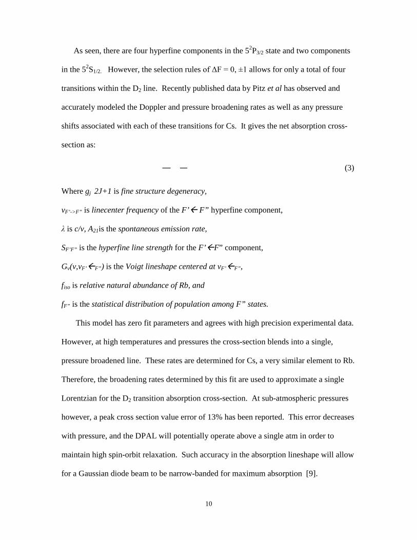
As seen, there are four hyperfine components in the 52P3/2 state and two components
in the 52S1/2. However, the selection rules of ΔF = 0, ±1 allows for only a total of four
transitions within the D2 line. Recently published data by Pitz et al has observed and
accurately modeled the Doppler and pressure broadening rates as well as any pressure
shifts associated with each of these transitions for Cs. It gives the net absorption cross-
section as:
(3)
Where gj 2J+1 is fine structure degeneracy,
vF’->F” is linecenter frequency of the F’ F” hyperfine component,
λ is c/v, A21is the spontaneous emission rate,
SF’F” is the hyperfine line strength for the F’F” component,
Gv(v,vF’F”) is the Voigt lineshape centered at vF’F”,
fiso is relative natural abundance of Rb, and
fF” is the statistical distribution of population among F” states.
This model has zero fit parameters and agrees with high precision experimental data.
However, at high temperatures and pressures the cross-section blends into a single,
pressure broadened line. These rates are determined for Cs, a very similar element to Rb.
Therefore, the broadening rates determined by this fit are used to approximate a single
Lorentzian for the D2 transition absorption cross-section. At sub-atmospheric pressures
however, a peak cross section value error of 13% has been reported. This error decreases
with pressure, and the DPAL will potentially operate above a single atm in order to
maintain high spin-orbit relaxation. Such accuracy in the absorption lineshape will allow
for a Gaussian diode beam to be narrow-banded for maximum absorption [9].

11
By narrow-banding the pump beam in such a way and maintaining proper buffer gas
to alkali concentrations, and assuming no lasing, the initial pump rate and spin-orbit
relaxation rate far exceed the spontaneous or stimulated emission rate on the lasing
transition. This leads to a saturated D2 transition and the upper two levels at their
Boltzmann distribution. In this instance the kinetics of the system can be modeled by the
following equations:
(4)
(5)
(6)
Where is the total alkali concentration, are the populations in the ground,
upper laser, and upper pump state respectively, are the degeneracies associated
with those states, ΔE is the energy split between the upper two levels, k is the Boltzmann
Constant, and T is temperature. In this instance two limits are being achieved
simultaneously, the “bleached” pump transition limit, and the quasi two-level (Q2L)
limit. The bleached limit corresponds to a fully saturated pump transition and the Q2L
refers to the dynamics when the spin-orbit relaxation rate far exceeds the spontaneous or
stimulated emissions rate on the lasing transition. Solving this system of equations gives
the pre-lasing populations of the three states involved, and as mentioned before, at room
temperature places over 45% of the population in the upper laser level, while leaving
only 17% in the ground. Such a high inversion allows for gain above threshold to be
achieved relatively easily. Figure 3 on the following page shows the inversion ratio
between the 2P1/2 and ground level as a function of cell temperature:

12
As shown, alkalis (specifically Rb), are capable of high inversions through a combination
of three factors: favorable degeneracy ratios between states, rapid interaction with buffer
gases, and a significant Boltzmann differential.
In order to ensure this inversion is maintained and accurately predict gain medium
kinetics precise knowledge of the dynamics between the alkali and buffer gas is requisite.
This dynamic enters the laser rate equations in the form of the spin-orbit mixing rate
coefficient, k32 with units of cm3/s. The product of k32 and the buffer gas concentration
(E), in cm-3, yields the number of collision induced energy transfers per atom per second.
Its role is shown explicitly in equation 7, which is a portion of the lasing mode rate
equation for the population density of the upper lasing state:
(7)
300 320 340 360 380 400 420 440
2.2
2.4
2.6
2.8
3.0
Alkali TemperatureK
N 2 N 1
Figure 3. Initial Population Inversion vs. Alkali Temperature

13
As shown, the spin-orbit mixing rate coefficient defines how quickly the upper two levels
of the system equilibrate. The factor of two in equation 7 is due to the 2:1 degeneracy
ratio between the hyperfine states of 52P3/2 and 52P1/2 in Rb, respectively. Theoretically
the rate constant is defined as:
(8)
Where Vavg is the average relative velocity of the collision pair, μ is the reduced mass of
the collision pair, (μ = [(MRbMMe)/( MRb+MMe)], and σ is the spin-orbit relaxation cross-
section. This rate has a published value of 5.2x10⁻¹⁰ cm3/s, and at 700 torr of buffer gas,
cycles each atom through the lasing process many millions of times per second [16].
This allows for relatively low alkali concentrations to create high power intracavity beam
intensities, potentially minimizing thermal management issues.
This spin-orbit kinetic process cannot be fully analyzed without an accurate account
of the alkali concentration. At projected operating temperatures alkalis are in their liquid
phase, and do not reach their boiling point until 1032 K. However, in liquid phase there
is still a small percentage of atoms in their gas phase due to the slight probability of Rb
atoms separating from the lattice by means of constructively interfering phonons,
localized “hot spots” within the liquid, or any other thermally induced energy influx. A
compilation of Rb data by Steck gives a rough guide to this percentage in terms of vapor
pressure in Torr and is given by equation 9 below:
(9)
where Pv is the alkali vapor pressure in Torr [13]. A graph of this pressure near projected
operating temperatures is shown here:

14
Figure 4. Rb Vapor Pressure vs. Temperature [13]

15
A final prerequisite for the feasibility of the DPAL to produce weapons grade
intensity and beam quality on target is high atmospheric transmittivity. Atmospheric
attenuation is devastating to the advantages of laser quality radiation, and can greatly
reduce the effective range of the weapon. Absorption bands of the atmospheres
constituent particles lead to diminishing intensity, dispersion, and diffraction causing a
relatively weak and dispersed radiative strike. However, at the operating wavelength of
the Rb based DPAL (795 nm), there is a transmission window with a transmittivity
coefficient of over 80%. That figure is the value for the transmission through the entire
atmosphere, holding promise that even higher transmission will occur for the projected
operating range of the ABL (~500 km). Figure 5 shows the atmospheric percent
transmission for a broad range of wavelengths given a Zenith angle of 20 degrees:
Figure 5. Atmospheric Transmittivity

16
Alkali earth metals have been chosen as the gain medium in the DPAL for a wide
variety of reasons. First, there is a strong foundation of knowledge regarding their
fundamental subatomic structure. Second, they possess remarkable QE, high absorption
probabilities, and are capable of creating large population inversions. Also, each atom is
capable of producing millions of laser photons per second through a high Boltzmann
differential and accessible spin-orbit relaxation. They are easily vaporized at modest
temperatures allowing for gas phase thermal management. They produce laser photons at
frequencies within atmospheric windows, leading to high intensity weapons grade power
on target. Finally, they are cheap, abundant and relatively easy to use, (albeit reactive to
atmospheric exposure). They hold promise for high power, compact, efficient, and cost
effective systems.
Diode Pumped Alkali Laser Technology
The DPAL has generated much attention from many institutions including The Air
Force Institute of Technology, Lawrence Livermore National Laboratory, University of
New Mexico, Air Force Research Laboratory (AFRL) Directed Energy Directorate,
Krupke Lasers and others. With so many entities in pursuit of realizing the potential of
this system much progress has been made. It should be noted however that the DPAL
technology is still in its early stages and there is still much design, engineering,
experimentation and ingenuity required before this dream becomes a reality. Presented
here is a review of publications pertaining to technological advancements of the DPAL.
Although gas phase lasers are inherently less effected by thermal heating, issues still
arise and a gain medium flow system has been successfully designed, developed and
demonstrated by AFRL. This system flows the alkali-buffer gas gain medium through

17
the resonator of the DPAL and carries away heat. By doing so, a fresh set of atoms is
ready for the absorption-relaxation phases of the 3-step cycle and atoms lost to effects
such as multi-photon absorption, collisional excitation into higher lying states, ionization
or other processes outside the 3 level model are flown out of the cavity [11]. This is a
significant first step towards achieving excellent beam quality at high laser powers.
A high efficiency Rb DPAL has been demonstrated with a linear optical slope
efficiency of 69%. In this setup, a static alkali/ethane/helium lasing vapor mix is pumped
with an approximately 1 MHz bandwidth diode laser achieving a maximum output power
of 490 mW. This was achieved with 400/50 Torr of ethane/helium and a 20% reflective
output coupler. It also achieved an optical-optical efficiency of 31.5% with a large
threshold of ~677 mW. Linear scaling on the efficiency was maintained showing the
spin-orbit relaxation rate was high enough to maintain a quasi two level system, resulting
in a proportional increase to laser intensity as input beam intensity is increased [8].
A second demonstration of a DPAL device by Sulham et al focusing on operating
high above threshold and achieved an output power of over 32 times threshold while
maintaining a linear slope efficiency between 39% and 49%. This places only 3% of the
efficiency loss due to threshold values. It also suggests that no second order kinetic or
optical processes are involved in this experimental setup, and with an output intensity of
over 20 kW/cm2 demonstrates relatively high output powers [13]. However, the pump
beam is pulsed with a 100 ns pulse width and may not accurately represent continuous
wave operation, since thermal effects would not be readily apparent. It is possible that
second order or nonlinear effects may not set in until a greater time span. Figure 6 at the
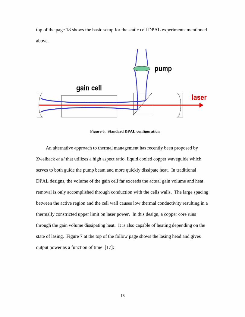
18
top of the page 18 shows the basic setup for the static cell DPAL experiments mentioned
above.
An alternative approach to thermal management has recently been proposed by
Zweiback et al that utilizes a high aspect ratio, liquid cooled copper waveguide which
serves to both guide the pump beam and more quickly dissipate heat. In traditional
DPAL designs, the volume of the gain cell far exceeds the actual gain volume and heat
removal is only accomplished through conduction with the cells walls. The large spacing
between the active region and the cell wall causes low thermal conductivity resulting in a
thermally constricted upper limit on laser power. In this design, a copper core runs
through the gain volume dissipating heat. It is also capable of heating depending on the
state of lasing. Figure 7 at the top of the follow page shows the lasing head and gives
output power as a function of time [17]:
Figure 6. Standard DPAL configuration

19
As seen on the left, an offset coolant channel penetrates the gain medium rapidly
dissipating or adding heat to the gain medium. The plot to the right, as interpreted by its
author, is best described by thermally induced fluxuations in Rb concentration. Initially,
Rb concentrations are below optimal, however through heating the vapor pressure is
increased until the most effective concentration for the input beam strength is reached.
Rollover begins as alkali concentration becomes high and the gain medium optically
thick. Eventually lasing ceases after the pump beam is unable to penetrate the length of
the gain cell and gain receeds below threshold. This design shows greater control over
thermal management and may also be capable of being expanded to a time varying
temperature control system that is based on the current output efficiency [17].
Since their advent in 2003, the DPAL has seen noteworthy improvement in its
realization. Early DPAL demonstrations achieved maximum output powers of 1 to 3
Watts. Currently operating CW DPALs are in the 100’s of Watts and the pulsed variety
Figure 7. Copper Waveguide Model and Results [17]

20
in the 10’s of kilowatts. Multiple initiatives into solving the thermal management issues
associated with the DPAL have shown success. And third, impressive slope efficiencies
have been observed in a variety of experiments. Research and design is ongoing and as
more data is collected and rates and quantities defined they can be integrated into the
model making it more precise and robust.

21
III. Methodology
Introduction
Presented here is a derivation from fundamental laser physics of the analytic model
developed initially by Dr. Gordon Hager and extended through the work of this thesis.
The model is implemented in “Mathematica”, a leading computation software package in
scientific academia. The initial derivation will neglect pump beam linewidth and derive
solutions which are based on a single frequency delta function input beam. Afterwards, it
will be shown that a frequency dependent pump beam intensity function is easily applied
to the solutions of this more simple case. The model incorporates all of the currently
published values for the various spectroscopic constants and broadening rates.
While this model is analytic in nature, it does rely on numerical integration of certain
functions, and some approximations are made. However, these functions are continuous
over the bounds of integration and have slopes much lower than the numerical integration
step size, giving confidence in resultant values. Also, the model only analyzes a Rb
based DPAL with an ethane/helium buffer gas mix. Approximations in regards to certain
effects being neglected or deemed insubstantial will be addressed as they arise.
As mentioned in the abstract, the model produces an output beam intensity function
dependent on seven input values. These include the input beam intensity, input beam
linewidth, the Rb concentration, ethane concentration, mirror reflectivitiy, cavity
transmittivity, and gain cell length. After incorporating all the fundamental aspects of the
physics involved, plots are generated through “Mathematica” of the various effects
changes in system parameters have on output beam intensity. The figure on the
following page highlights all the essential features included in the model.

22
Shown in the standard layout above, the model has yet to incorporate spatial
dynamics and is independent of cavity design. It is currently only capable of predicting
output intensities, not net output power, cavity mode, or output beam quality. Being so,
design engineers planning a system based on the results of the model will have freedom
in design, constraining themselves only to meeting the parametric settings of the desired
predicted output intensity. The pump linewidth extension has yet to be made on the
lasing transition and its cross-sectional value is taken at its linecenter peak value. The
table on the following page is to be used as reference throughout the derivation of the
model and lists all symbols used with their definition and value (if applicable).
Figure 8. Model Dependent Variables

23
Symbol Definition Value Units
N1 concentration of atoms in ground state variable cm-3 N2 concentration of atoms in the 52P1/2 state variable cm-3 N3 concentration of atoms in the 52P3/2 state variable cm-3 Ntot alkali concentration variable cm-3
σ21 absorption cross section on the lasing transition *4.80x10⁻¹³
(linecenter) cm2
σ31 absorption cross section on the pump transition *4.92x10⁻¹³
(linecenter) cm2
Ω longitudinally averaged two-way intracavity pump beam
intensity variable W/cm2 h Planck’s Constant 6.626x10⁻³⁴ J-s ν21 frequency of the laser beam 3.774x10¹⁴ Hz ν31 frequency of the pump beam 3.846x10¹⁴ Hz k32 spin-orbit mixing rate (Ethane partner) 5.2x10⁻¹⁰ cm3/s t21 radiative lifetime of upper laser level 27.7 ns t31 radiative lifetime of upper pump level 26.23 ns Ψ intracavity average two-way laser intensity variable W/cm2 E Ethane concentration variable cm-3 lg gain cell length variable cm R net cavity reflectivity variable N/A T net cavity transmission variable N/A K Boltzmann constant 1.38065x10⁻²³ J/K T Gain cell temperature variable K gth threshold gain variable cm-1 Ipin input beam intensity variable W/cm2 C speed of light (in vacuum) 3.0x10⁸ m/s λ31 pump wavelength 780.026 nm λ21 laser wavelength 794.76 nm Δν31 pump beam bandwidth variable Hz He Helium concentration variable cm-3 g1 degeneracy of ground state 2 N/A g2 degeneracy of upper laser level 2 N/A g3 degeneracy of upper pump level 4 N/A
Table 3. Model Variable Definitions (Rb DPAL)

24
Longitudinally Averaged Two-Way Intracavity Pump Beam Intensity
We begin by defining the intracavity pump beam intensity. Consider the interaction
between the pump beam at each transition through, or reflection off of, a component of
the cavity. The intensity off the initial interaction with the beam splitter defines Ipin, from
there the beam is incident on the first wall of the gain cell, receiving a transmission loss
defined by tp, resulting in an initial inner cell intensity of tpIpin. As the beam progresses
through the gain cell, it receives a Beer’s Law exponential gain given by:
(10)
where g31 is the gain on the pump transition. After exiting the cell another transmission
loss is taken as well as a reflectivity loss defined as rp. Finally, before re-entering the cell
it experiences another transmission loss as it passes through the cell wall. This gives the
intensities of the two initial input beams incoming from both ends of the cell as:
(11)
(12)
where I+ is the initial incident pump beam intensity and I – is the intensity of the input
beam after a single pass a reflection back into the gain medium. Figure 9 below shows
the input beam intensity at each transition for a single round trip pass [2].
Figure 9. Round Trip Pump Beam Intensity

25
Assuming the beam is highly attenuated after a single round trip, the longitudinally
averaged intracavity pump beam intensity can be defined by integrating the sum of these
two incident beams across the length of the gain medium, and averaging the result. The
explicit derivation is shown here:
(13a)
(13b)
(13c)
Substituting values from equations 11 and 12 for I+ and I – yields:
(13d)
Ignoring transmission losses and assuming 100% pump beam reflectivity simplifies this
equation to:
(13e)
Considering the beam is highly attenuated after its first pass and the first transmission
loss could be incorporated into the initial beam intensity, the approximation in eqn. 13e
will be used to define Ω. In the same manner output laser intensity can be defined in
terms of the average intracavity lasing intensity by [2]:
(14)
26
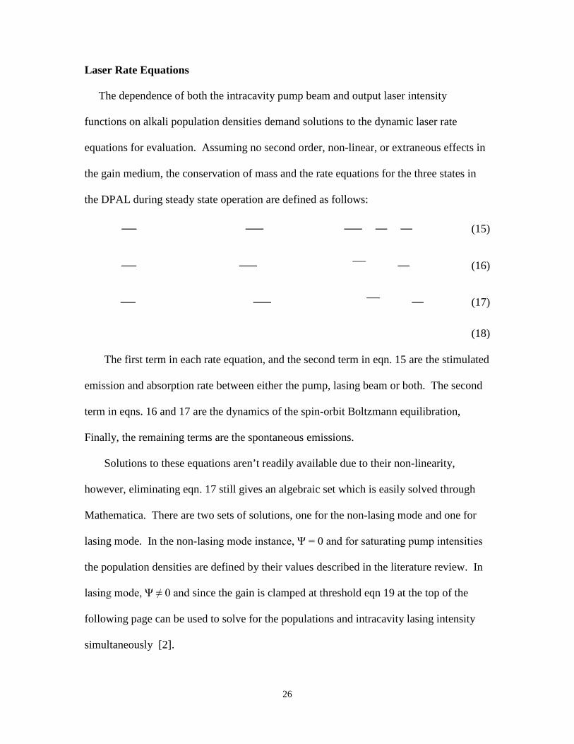
Laser Rate Equations
The dependence of both the intracavity pump beam and output laser intensity
functions on alkali population densities demand solutions to the dynamic laser rate
equations for evaluation. Assuming no second order, non-linear, or extraneous effects in
the gain medium, the conservation of mass and the rate equations for the three states in
the DPAL during steady state operation are defined as follows:
(15)
(16)
(17)
(18)
The first term in each rate equation, and the second term in eqn. 15 are the stimulated
emission and absorption rate between either the pump, lasing beam or both. The second
term in eqns. 16 and 17 are the dynamics of the spin-orbit Boltzmann equilibration,
Finally, the remaining terms are the spontaneous emissions.
Solutions to these equations aren’t readily available due to their non-linearity,
however, eliminating eqn. 17 still gives an algebraic set which is easily solved through
Mathematica. There are two sets of solutions, one for the non-lasing mode and one for
lasing mode. In the non-lasing mode instance, Ψ = 0 and for saturating pump intensities
the population densities are defined by their values described in the literature review. In
lasing mode, Ψ ≠ 0 and since the gain is clamped at threshold eqn 19 at the top of the
following page can be used to solve for the populations and intracavity lasing intensity
simultaneously [2].

27
(19)
The simultaneous solutions to the the steady state laser mode population densities and
intracavity laser beam intensity are given by:
(20)
(21)
Transcendental Solution
We now have solutions to the independent variables (population densities) for the
intracavity pump beam, intracavity lasing beam, and output laser intensity. However,
these variables are themselves dependent on the averaged intracavity pump beam
intensity. This causes the solution for Ω to be transcendental in nature, as in it is
inherently a function of itself. Rewriting equation 13e to show this dependence explicitly:
(24)
(22)
(23)

28
As seen, in order to evaluate and obtain values for the intracavity pump intensity an
input value for said intensity must determined. It is only when both the independent
variable value for Ω and the function output value itself are equal is there a solution.
These are found by solving the planar intersection between f(Ω) = Ω and Ω. The graph
below is an example of this intersection for typical DPAL parametric settings.
The intersection of the two functions shown above are the solutions, given the
baseline parametric settings, to the intracavity longitudinally average pump beam
intensity for Ipin values ranging from 0 – 20000 W/cm2. The model solves this
intersection problem by solving for Ω in the root equation below:
– (25)
Figure 10. Transcendental Intersection

29
In doing so explicit values which can be used as input into the intracavity laser
intensity equation can be found and the model is capable of predicting output laser beam
intensities based on the seven fundamental parameters within the system. Figure 11
below gives Ω values for a range of input beam intensities with the baseline parametric
settings found in table 4.
Given these solutions we rewrite the output beam intensity as an explicit function of
input beam intensity, and thereby completing the frequency independent part of the
model. With this ability, we now have a “black box” capable of taking in a set of
parametric settings and giving us our desired result, output beam intensity, explicitly:
(26)
Figure 11. Ω vs Ipin

30
Frequency Dependence of the Pump Transition
As mentioned, matching the pump beam spectral profile to the absorption cross-
section lineshape is paramount for optimal efficiency. In order to model this, we must
assign a frequency dependence to the absorption cross-section (σ31) and the input beam
intensity (Ipin). This is done by appending normalized frequency distribution functions
onto the mentioned existing values:
(27)
(28)
Where fpump is a normalized Gaussian Distribution and f31 is a pressured broadened
Lorentzian Distribution. They are defined explicitly in equations 29 and 30.
(29)
(30)
For baseline operating conditions of 600 Torr of Ethane and Rb vapor concentrations
corresponding to 393.15 K the pressure broadened width of the absorption cross section
has a FWHM value of 19.73 GHz. By setting the diode FWHM to this optimistically
narrow bandwidth excellent spectral overlap is achieved as shown in figure 12 below:
Figure 12. D1 Spectral Overlap [3]

31
The majority of the produced results set the FWHM of the absorption cross section to
a predetermined value not coupled to cell temperature or buffer gas concentration.
However a few plots incorporate the broadening effects associated with increased
pressure and cell temperature, for those the FWHM is defined as:
(31)
Where is the published broadening rate, is the temperature at which the rate was
measured, E is the ethane concentration (or corresponding gas) and T is the current
DPAL operating temperature.
Due to the frequency dependence of the input beam and absorption cross-section, the
first term in equation 15 becomes an integral over frequency and algaebraic solutions to
the rate equations cease. However, a solution to the problem has been arrived through
redefining the rate equations with an overall pump beam interaction term Ωf. It begins by
adding a frequency dependence to the single frequency solution of Ω:
(32)
Multiplying by the denominator (except for lg) and integrating over frequency gives:
(33)
The term on the left of eqn. 33 is the frequency dependent absorption and stimulated
emission rate for the lasing transition, and is the term limiting an algebraic solution. By
defining Ωf as this and substituting it into the rate equations solutions are once again

32
obtained for the population densities, however this time they are dependent on Ωf. This
once again leads to a transcendental equation for Ωf, explicitly:
(34)
Solutions are again obtained through the root equation method, and new population
density functions are generated independent of Ωf, and are now functions of Ipin. By
doing so the “black box” is once again established and the frequency addition to the
pump interactions has been accomplished. The output laser intensity is now a function of
pump beam bandwidth as shown in eqn. 35.
(35)
With the ability to predict output laser intensity with 8 dimensions of variability in a
quasi-analytic fashion the DPAL three level model is an excellent tool for analysis of
projected future technologic endeavors. The few approximations that have been made
are minimized or have been deemed insubstantial. For a complete layout of the code,
with a brief Mathematica tutorial, see appendix b.

33
IV. Results and Analysis
Introduction
The code generates 2D and 3D plots describing laser performance characteristics
including efficiency, pump beam output intensity, population density ratios, direct
comparisons to single and multi-frequency cases, and others. The single frequency
results are presented first and will be used for comparison with the broadband pump
beam results. Each plot is accompanied with an analysis of the results given the
implications that the graphs trends have on laser characterization. The 3D plots are
capable of showing the simultaneous effect changes in multiple systems parameters have
on the laser output making it easier to assign significance to each input variable.
The graphs generated are based on a set of “baseline” parametric settings. These
correspond to recent experimental operating conditions and the values for the frequency
independent segment of the code are given in the table below. The Rb concentration
corresponds to a cell temperature of 393.15 K, the ethane concentration corresponds to a
partial pressure of 300 Torr.
Variable Value Units
lg 2 cm
Ntot 1.85x1013 cm-3
E 9.66x1018 cm-3 r 0.2 N/A t 0.975 N/A
Table 4. Baseline Parameters - Frequency Independent Case
34
Single Frequency, No Lasing Results
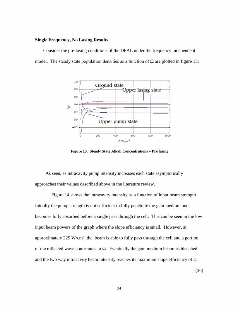
Consider the pre-lasing conditions of the DPAL under the frequency independent
model. The steady state population densities as a function of Ω are plotted in figure 13:
As seen, as intracavity pump intensity increases each state asymptotically
approaches their values described above in the literature review.
Figure 14 shows the intracavity intensity as a function of input beam strength.
Initially the pump strength is not sufficient to fully penetrate the gain medium and
becomes fully absorbed before a single pass through the cell. This can be seen in the low
input beam powers of the graph where the slope efficiency is small. However, at
approximately 225 W/cm2, the beam is able to fully pass through the cell and a portion
of the reflected wave contributes to Ω. Eventually the gain medium becomes bleached
and the two way intracavity beam intensity reaches its maximum slope efficiency of 2.
(36)
Figure 13. Steady State Alkali Concentrations – Pre lasing

35
Single Frequency, Lasing Mode Results
Presented in this section are the results for the frequency independent, steady state
lasing mode case. The baseline parameters are the same from the previous section, and it
is shown that these results coincide well the the pre-lasing mode results. Analysis of the
frequency independent case will build intuition on the dynamics and interactions of the
system paving the way for a clearer view of the effect that broadening the pump beam has
on the DPAL. Recall in this instance the interaction between the pump beam and the
system is represented with a delta function in frequency input intensity centered on the
peak absorption cross-section value. Being so, we assume this represents the upper limit
on absorption and for certain settings efficiency, output beam strength, and inversion
ratios for a given input beam intensity. Figure 15 on the following page shows the
oscillating intracavity laser intensity as a function of the intracavity beam intensity.
Figure 14. Pre-Lasing Intracavity Pump Beam Intensity – Frequency Independent

36
Initially the pump beam is unable to reach threshold and Ψ is undefined. However,
at an Ω value of 40.04 W/cm2 threshold is reached and lasing begins. The linear slope
regime above represents the Q2L behavior with the spin-orbit relaxation able to keep up
with the pump and laser transitions. Rollover occurs as these radiative transfer rates
dominate the dynamics and the buffer gas is unable to equilibrate the alkali in time for the
relatively high oscillating Ψ value to see an inversion. An asymptotic limit representing
a bleached laser transition begins to develop at higher Ω values. This threshold value
corresponds well with the calculated threshold value of 40.3 W/cm2 for the no lasing
case, showing the model is well coordinated and precise.
0 2000 4000 6000 8000 10000 12000
3000
4000
5000
6000
7000
Wcm2
Wcm2
Figure 15. Intracavity Laser Intensity – Frequency Independent

37
The plot of the intracavity pump beam intensity as a function of input beam strength
for the lasing case is similar to the non lasing except the curvature is described by
different phenomena. As seen below, once again Ω is slow to initially rise, then turns and
hits a maximum slope efficiency. Initially the spin-orbit rate is able of cycling the atoms
into the upper lasing state where the inversion with ground maintains amplification of the
oscillating laser intensity. However, for the defined parametric settings, absorption
begins to cease as the spin-orbit rate is unable to funnel atoms into the lower fine-
structure level. This results in a linear slope efficiency of over 100%. This plot is shown
in Figure 16 below:
Figure 16. Intracavity Pump Intensity – Frequency Independent

38
The dramatic effect that varying ethane concentration has on output intensity and
slope efficiency is readily seen in Figure 17 shown here:
As seen, once the maximum spin-orbit relaxation rate is reached rapid rollover
begins as the cyclic photon engine begins to break down, and bottlenecking in the upper
pump state occurs. While increasing the buffer gas pressure seems like the apparent
solution, broadening rates on the cross-sections must be considered and maintaining a
single mode laser intensity becomes more challenging as more and more modes rise
above threshold. There is also potential for cross-section overlap at high enough
pressures which would greatly reduce efficiency of the ability to lase.
As an inverse, consider holding the ethane pressure a constant and varying alkali
concentration. In doing so similar results are produced as can be seen on Figure 18
presented here:
0 2000 4000 6000 8000 10000 12000
0
2000
4000
6000
8000
Ipin Wattscm2
W
attscm2
vs IpinFrequency Independent, Lasing
500Torr
400Torr
300Torr
200Torr
100Torr
Figure 17. Ethane Variation – Frequency Independent

39
When the alkali number density is low, the cell becomes easily bleached by the
incident pump beam and the majority of the incident photons are wasted. However, the
Q2L limit is maintained at higher input beam intensities and a linear slope efficiency
maintained. The concentrations are not so optically thick as to limit lasing at such high
pump intensities.
Window transmittivity also plays a vital role in slope efficiency. Gain is dependent
on the negative of the log of the transmission factor, implying that as transmittivity
increases, gain becomes more negative.
0 2000 4000 6000 8000 10000120000
2000400060008000
10000
Ipin Wattscm2
II las
eW
attscm2
IIlase vs IpinFrequency Independent, Lasing3.410132.810132.210131.6101311013R
Figure 18. Rubidium Variation – Frequency Independent
Rb Concentration (cm-3)
40
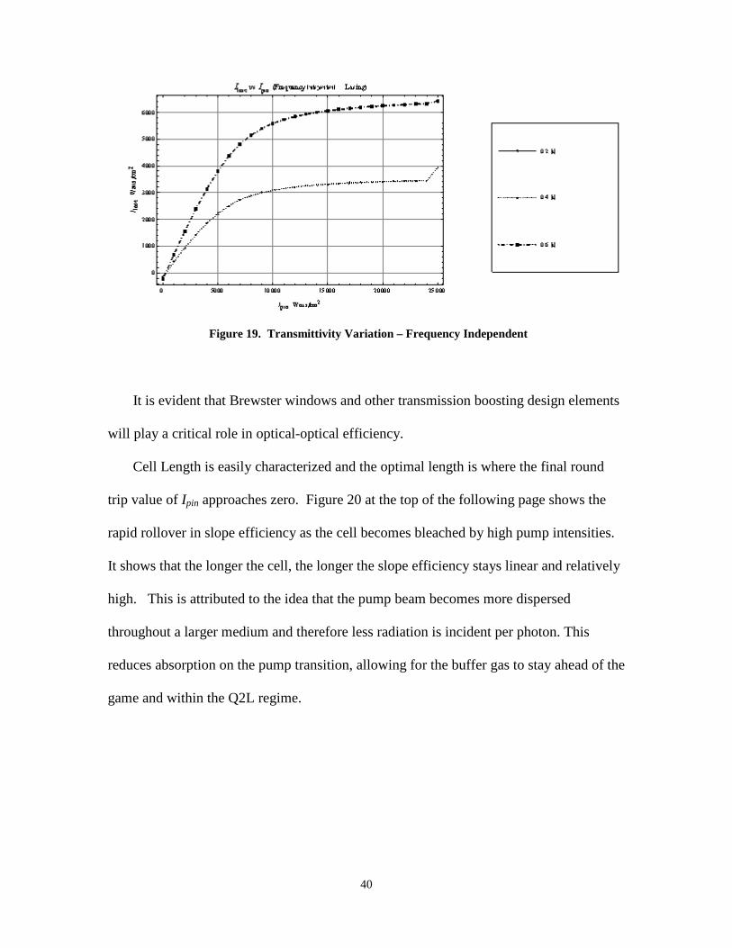
It is evident that Brewster windows and other transmission boosting design elements
will play a critical role in optical-optical efficiency.
Cell Length is easily characterized and the optimal length is where the final round
trip value of Ipin approaches zero. Figure 20 at the top of the following page shows the
rapid rollover in slope efficiency as the cell becomes bleached by high pump intensities.
It shows that the longer the cell, the longer the slope efficiency stays linear and relatively
high. This is attributed to the idea that the pump beam becomes more dispersed
throughout a larger medium and therefore less radiation is incident per photon. This
reduces absorption on the pump transition, allowing for the buffer gas to stay ahead of the
game and within the Q2L regime.
Figure 19. Transmittivity Variation – Frequency Independent

41
Broadband Pump, Lasing Mode Results
With confidence in the single frequency model the addition of pump bandwidth has
been made and the results are shown here. Consider first only varying pump beam
bandwidth. It is apparent from Figure 21 on the following page that matching the
bandwidth to the absorption has a strong effect on optical-optical efficiency. It also has
effects on the rollover point, population inversion and 3D plots showing the effects of
bandwidth on the other parameters are analyzed. Comparison to the single frequency
case shows a reduction in efficiency as expected. The graph on the following page gives
our frequency dependent pump beam intensity as a function of Ipin for a range of spin-
orbit pressures.
0 2000 4000 6000 8000 10000 12000
0
2000
4000
6000
8000
10000
Ipin Wattscm2
II las
eW
attscm2
IIlase vs IpinFrequency Independent, Lasing
5 cmlg4 cmlg3 cmlg2 cmlg1 cmlg
Figure 20. Cell Length Variation – Frequency Independent

42
The highest bandwidth (500 GHz), has relatively low slope efficiency as a somewhat
small proportion of the photons are within the absorption profile of the transition. As
bandwidth decreases, slope efficiency rises. This is caused by the increase in absorption
and a more rapid approach to the bleached transition limit. As you can see, the 10 GHz
pump beam mimics the single frequency case in that around 5200 W/cm2 the cell
becomes bleached and Ωf approaches its limiting value of 2Ipin. However, all other
bandwidths excluding the 500 Ghz have intracavity pump beam intensities greater than
Ipin, implying that absorption towards a saturated state is consistent with those
bandwidths. Given that more broadened pump beams can saturate the D2 transition, there
may be less of a demand to pursue narrowbanded diode stacks . An investigation into
overall efficiency between narrowbanding the diode bars or pumping broadband may
prove worthwhile. A second plot emphasizing the importance of spectral overlap is seen
at the top of the following page.
0 5000 10000 15000 20000 250000
10000
20000
30000
40000
Ipin Wattscm2
W
atts cm2
vs IpinFrequency Dependent, Lasing
500GHz
200GHz
100GHz
50GHz
10GHz
Figure 21. Ω vs Ipin – Frequency Dependent
43
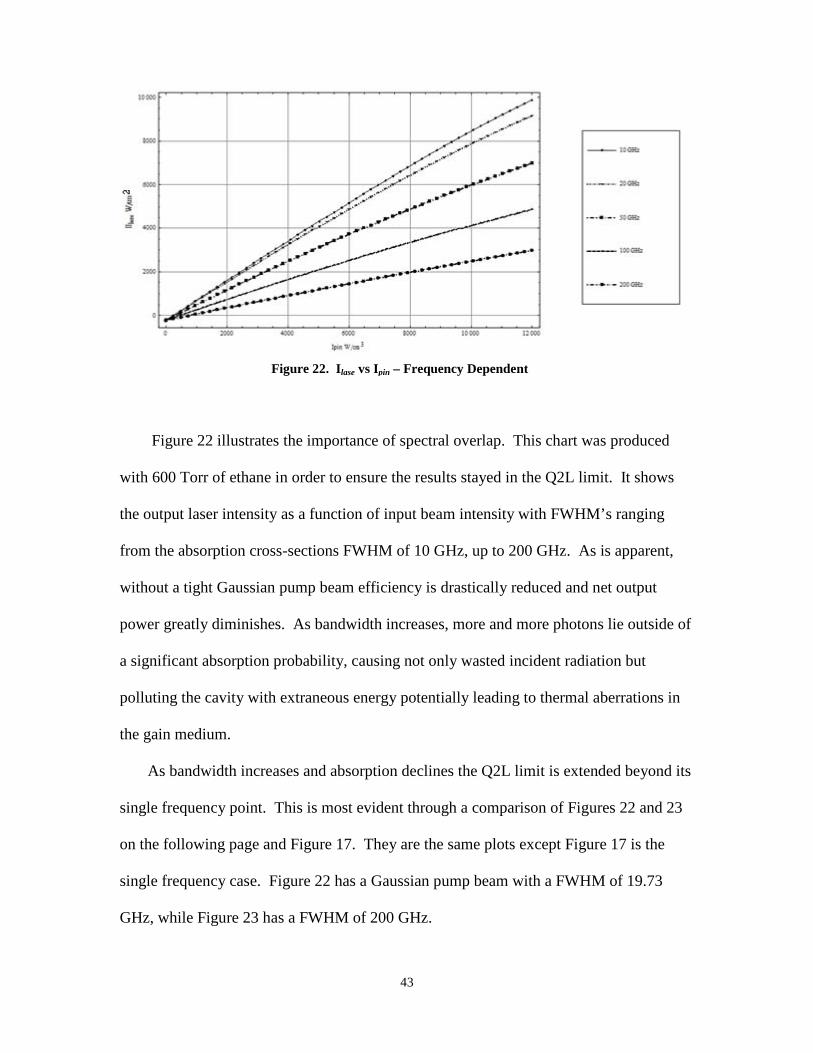
Figure 22 illustrates the importance of spectral overlap. This chart was produced
with 600 Torr of ethane in order to ensure the results stayed in the Q2L limit. It shows
the output laser intensity as a function of input beam intensity with FWHM’s ranging
from the absorption cross-sections FWHM of 10 GHz, up to 200 GHz. As is apparent,
without a tight Gaussian pump beam efficiency is drastically reduced and net output
power greatly diminishes. As bandwidth increases, more and more photons lie outside of
a significant absorption probability, causing not only wasted incident radiation but
polluting the cavity with extraneous energy potentially leading to thermal aberrations in
the gain medium.
As bandwidth increases and absorption declines the Q2L limit is extended beyond its
single frequency point. This is most evident through a comparison of Figures 22 and 23
on the following page and Figure 17. They are the same plots except Figure 17 is the
single frequency case. Figure 22 has a Gaussian pump beam with a FWHM of 19.73
GHz, while Figure 23 has a FWHM of 200 GHz.
Figure 22. Ilase vs Ipin – Frequency Dependent

44
Shown above are the effects of ethane concentration on output intensity for a 19.73
GHz input beam. Through comparison with Figure 17, it is shown that the linear slope
efficiency is maintained for larger values of Ipin. This is due to the reduction in absorbed
beam intensity as bandwidth is increased. This can be seen to an even greater extent in
Figure 24 below (200 GHz input beam bandwidth):
0 5000 10000 15000 20000 25000
0
2000
4000
6000
8000
Ipin Wattscm2
I lase
Watt
scm2Ilase vs IpinFrequency Dependent, Lasing
500Torr
400Torr
300Torr
0 5000 10000 15000 20000 25000
0
1000
2000
3000
4000
5000
Ipin Wattscm2
I lase
Watt
scm2
Ilase vs IpinFrequency Dependent, Lasing
500Torr
400Torr
300Torr
Figure 23. Ethane Variation – Frequency Dependent (19.73 GHz)
Figure 24. Ethane Variation – Frequency Dependent (200 GHz)

45
The reflectivity of the cavity at the lasing wavelength seems to play a rather
insignificant role in output beam intensity. This may be attributed the extremely high
gain nature of the alkali gain medium and its ability to reach threshold regardless of
cavity reflection. The only obvious yet significant effect is seen when r = 1.0, or
complete reflection back into the cavity. This result strengthens the confidence in the
model as another intuitive result is produced as expected. Figure 25 show output
intensities for reflectivities ranging from 0.2 – 0.5. The zero output intensity straddles
the axis and is unseen but present on a color graph.
As seen, reflectivity within the cavity slightly effects slope efficiency. It does not seem
to effect the rollover effect or even maximize output beam intensity. This strengthens the
idea that the key rate or dynamic of the system is the spin-orbit relaxation rate.
0 5000 10000 15000 20000 25000
0
1000
2000
3000
4000
5000
6000
Ipin Wattscm2
I lase
Watt
scm2
Ilase vs IpinFrequency Dependent, Lasing
0.5r0.35r0.1r
Figure 25. Reflectivity Variation – Frequency Dependent

46
With this in mind a new parameter, Δ, is defined as N3/N2. It represents how close
the upper two laser levels are to their Boltzmann Distribution, or how close the system is
to operating in the Q2L regime. To see how the pump bandwidth effects this ratio, a 3D
contour plot with Δvpump and Ipin as the independent variables is generated and shown
below. The upper bound to the Boltzmann Equilibrated ratio for baseline parametric
settings is set at Δ = 1.73.
As seen pump bandwidth plays a significant role in defining Δ. At lower
bandwidths, Δ rises more quickly as expected through a higher net absorption. It
continues to stay above higher bandwidth values for the same pump intensity but rises
more slowly as Δ approaches its upper limit. This may be attributed to the decreased
Figure 26. Δ -Bandwidth Variation – Frequency Dependent
(Hz
W/cm2
47
percentage of the populations out of equilibrium which may reduce the buffer gas
effective equilibrium rate. At high pump bandwidths the rise in Δ is linear corresponding
to the Q2L regime. In this case as more photons are absorbed into the upper lasing level
there are more opportunities for the buffer gas to equilibrate with the alkalis in this state.
It also shows that this rate is able to keep up with the stimulated emission rate on the
lasing transition.
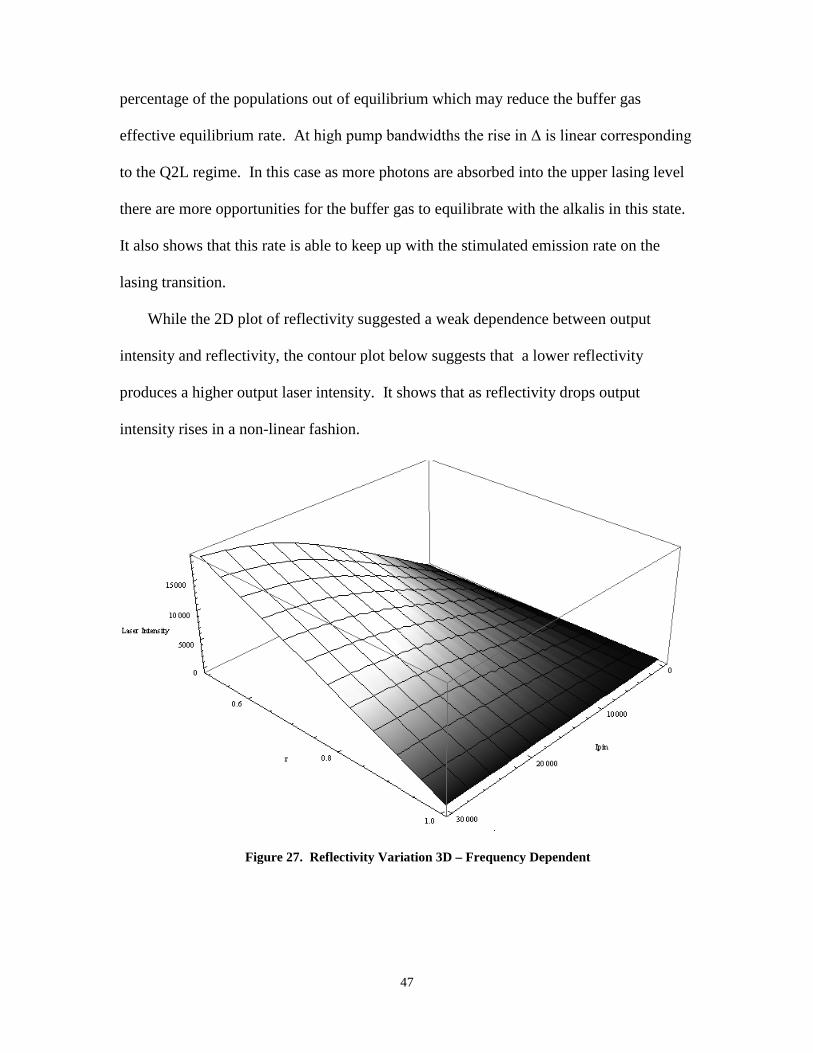
While the 2D plot of reflectivity suggested a weak dependence between output
intensity and reflectivity, the contour plot below suggests that a lower reflectivity
produces a higher output laser intensity. It shows that as reflectivity drops output
intensity rises in a non-linear fashion.
Figure 27. Reflectivity Variation 3D – Frequency Dependent

48
As seen maximum laser intensity is achieved at zero reflectivity. This once again
suggest alkalis possess extremely high gain and a single ASE output beam maybe be
capable of producing higher intensities than an oscillating laser cavity. However, for
high beam quality a proper single mode resonator should be designed with a relatively
low reflectivity.
Parametric efficiency studies have been conducted generating DPAL efficiency plots
for a range of input beam strengths, buffer gas concentrations and pump beam bandwidth.
Figure 25 below represents the optical-optical efficiency for a DPAL operating with a 10
kW input beam, 300 Torr of Ethane and 50 Torr He. The results incorporate the
broadening rates recently published by Pitz et al.
DPAL efficiency is plotted against the natural log of the Rb concentration and the
ratio between the pump and absorption cross section bandwidth. As expected, efficiency
depends highly on bandwidth. This graph also shows the effects of high Rb concentration
Figure 28. DPAL Efficiency – Frequency Dependent

49
on output. At the lower Rb concentrations, the pump beam is fully absorbed and slope
efficiencies are linear and high for each given bandwidth. Near the center value of the
Rb concentration efficiency drops as the gain medium becomes optically thick for a 10
kW input beam. This rollover however occurs at higher and higher Rb concentrations as
bandwidth in increased, as expected.
As mentioned above reflectivity plays a key role in determining output beam
strength. Presented below are the output intensities for a 80 kW input beam at various
bandwidths. Once again, as bandwidth rises, output drops.
This plot reinforces the results of the 3D reflectivitiy contour plot above in that
output intensity rises as reflectivity drops. However, eventually at high enough pump
intensities these curves converge into a single line. This probably represents a pump
beam intensity that bleaches the pump transition at all bandwidths. Figure 30 on the
following page gives the output intensity vs reflectivity for a 100 kW input beam, and
Figure 29. Reflectivity Variation 2D – Frequency Dependent

50
shows this effect. The model uses a baseline value for cavity reflectivity of 0.2,
corresponding to an efficiently designed laser system. At r = 0.2, there is still high output
intensities but with the ability to potentially create a resonating, single mode, diffraction
limited output beam.
As seen, at high pump intensities, the effects of bandwidth become insignificant due to
saturation. This effectively reduces the system to is frequency independent model and
solutions converge upon the lowest bandwidth instance.
One particular value of interest when analyzing pump bandwidth effects on laser
performance is the ratio between the frequency independent intracavity pump beam
intensity (Ω) and the frequency dependent intracavity pump beam intensity (Ωf).
Explicitly, Gamma is defined as:
(36)
Figure 30. DPAL Efficiency – Frequency Dependent

51
Intuitively one would believe that the frequency independent intracavity pump beam
intensity is bounded to be always greater than the frequency dependent case. However,
upon execution of the code the results are somewhat counter-intuitive. Figure 31 Gamma
at a variety of pump bandwidths for the baseline parametric settings.
And the same plot again for a more pressurized (500 Torr) gain cell:
0 5000 10000 15000 20000 250000.0
0.5
1.0
1.5
2.0
2.5
Ipin Wattscm2
vs IpinFrequency Dependent, Lasing, 300Torr
500GHz
200GHz
100GHz
50GHz
10GHz
0 5000 10000 15000 20000 25000
0
1
2
3
4
5
6
7
Ipin Wattscm2
vs IpinFrequency Dependent, Lasing, 500Torr
500GHz
200GHz
100GHz
50GHz
10GHz
Figure 31. Gamma – 300 Torr Ethane
Figure 32. Gamma – 500 Torr Ethane

52
Figure 33 shows the cause for Gamma dropping below 1. Initially the broadband pump
has a greater slope efficiency, caused by a reduction in absorption. However, at higher
pump intensities and saturated transition conditions the single frequency case approaches
is intracavity slope limit of 2Ipin, while the broadband case maintains a lower slope . At
around 15000 W/cm2 the single frequency rate has bleached the transition wheeras the
broadband case has not, leading to a greater slope efficiency. Returning again to laser
intensity, Figure 34 shows output intensity as a function of Rb concentration for a set of
pump bandwidths:
0 10000 20000 30000 400000
20000
40000
60000
80000
Ipin Wattscm2
vs IpinLasing, 500Torr
f
0 20 40 60 80 100 120 140
0
1000
2000
3000
4000
LogRbcm3
I lase
Wattscm2
Ilase vs LogRbFrequency Dependent, Lasing, 5000kWInput Beam
500GHz
200GHz
100GHz
50GHz
10GHz
Figure 34. Ilase vs. Log[Rb] – 500 Torr Ethane
Figure 33 - Ω vs Ipin 500 Torr Ethane (500 Ghz)

53
As is apparent in the graph, there is an optimal combination of alkali concentration,
and bandwidth which maximizes output and this combination points directly at low
bandwidth. At any given Rb concentration, the lowest bandwidth has the highest output
intensity, and at 10 GHz the appropriate Rb concentration results in an optical to optical
efficiency of about 80%. A second plot of Г vs γ for a family of pump bandwidths is
shown at the top of the following page. In order for the pump beam to drive the system it
must excite quicker than the lasing beam relaxes. In order to do so it must get absorbed
which is evident in Figure 34. At lower bandwidths Δ maintains an inversion and there is
bottlenecking at the upper pump state. This is a potential source of inefficiency and
further studies of a Δ for max efficiency may prove beneficial.
As shown, Δ decreases as the spin orbit rate increases, or as Ethane is added to the
system. A low Δ is good for efficiency but one that is too low may limit laser
performance.
0 1109 2109 3109 4109 5109 6109
1.0
1.2
1.4
1.6
s1
vsFrequency Dependent, Lasing, 5000kWInput Beam
500GHz
200GHz
100GHz
50GHz
10GHz
Figure 35. Δ – 300 Torr Ethane

54
The model is capable of producing a variety of results that can be used to analyze
and more intuitively understand the dynamics and various interactions of the system. By
accurately predicting the output beam intensity based on the fundamental elements of any
laser system, parametric solutions can be obtained upon which engineers can base their
designs.

55
V. Conclusions and Discussion
With the results of the model readily available and interpretable, conclusions on the
effects of broadband pumping are made. Also discussed are various effects between the
other independent variables. Third, issues with the approximations made are addressed
and finally, suggestions for future work on the model are made.
In essence, a broadening of the pump bandwidth offers very little towards achieving
maximum laser performance. As seen, as bandwidth increases, output laser intensity
decreases. Given that an objective of the DPAL is cost efficiency and low power-usage,
maximizing pump absorption is critical. However, the model does show that a very high
efficiency is theoretically possible, (albeit an engineering feat yet to be seen). There are
also certain cases where it may be possible for a more broad banded beam to actually be
more efficient, as is seen in Figure 21.
While it may seem intuitive, in a quantum mechanical sense, that any broadening of
an energizing spectral source will reduce efficiency, the current state of affairs regarding
diode stacks puts their bandwidths in the 100’s of GHz. With this in mind, if demand for
output power begins to heavily outweigh efficiency concerns, systems can be designed
based on the appropriate pump beam interaction, allowing the model to “pave the way”
for future progress. The model is also an open book without an ending and is capable of
become far more robust, accurate, precise and efficient.
As seen throughout the data, there must be a merger between all system parameters
in order to maximize performance. However, it was shown that some variables have a
greater influence than others. For example, reflectivity plays a minor role in determining
overall performance whereas buffer gas concentrations are far more critical. Bandwidth
56
plays a significant role however in practicality it seems as if it would be easier to simply
increase the pump intensity rather than adjust the ethane concentration. Cell length in the
standard DPAL design is held constant and the various other parameters can be adjusted
to make the most out of any length cell. In this author’s opinion, the system primarily
comes down to alkali and buffer gas concentrations, and pump beam intensity.
While the model is quasi-analytic, founded in laser engineering, and compares well
with experimental data, it lacks a sense of completeness or of an all encompassing
simulation of a true laser system. In a way, it is an algorithm reduced to the key elements
of any laser system, a simplification, an “ideal” representation of a far more detailed
phenomenon. Of greatest concern is the idea that all the alkalis reside in one of only
three possible states ( for Rb: 52P3/2, 52P1/2 or 52S1/2). Recently collected data suggests
that alkali’s, upon being excited to the 52P3/2 state experience a myriad of kinetic
processes and excitations before fluorescing back to ground. This results in “spreading
out” of the alkalis atoms into the various electron states. Fluorescence of a laser pumped,
vacuum sealed, thermally insulated Rb cell was collected by means of an optical cable
and a 0.3 M spectrometer. A series of data collections were undertaken to observe the
intensity fluctuations of the various Rb emission lines as a function of Rb concentration
and incident beam intensity. For each set the Rb vapor was subject to high intensity,
pulsed radiation in resonance with the D2 transition. A Grotrain Diagram displaying the
various observed emission lines is shown on the following page.

57
Figure 36. Grotrain Diagram – Laser Pumped Rb Fluorescence

58
As one can see, many different energy levels become populated solely from pumping
on the D2 line. A closer inspection of Figure 29 reveals that all dipole allowed transitions
are observed and even some non-dipole allowed. A detector with a larger bandwidth may
reveal even more Rb emissions.
A second issue with the model is that it makes great strides in an effort to maintain its
quasi-analytic nature. However, at times, this author feels too much of the physical
phenomena occurring in the laser system is ignored or deemed insignificant. In the
derivations of the longitudinally averaged two way intracavity pump beam intensity
certain terms are ignored or neglected for simplicity. This author suggests that one
should take advantage of the computational power accessible by AFIT and other facilities
to produce a more thorough account of the interactions within the system.
Even so, the model still makes accurate predictions and encompasses all of the
fundamental laser physics involved with the DPAL. It is an excellent tool for analysis,
exploration, brainstorming, and there are many upgrades that could begin tightening the
gap begin the model and the lab. First, extending the frequency dependence of the pump
transition to the lasing transition would produce more accurate and fundamentally sound
results. Second, considering numerical integration is already implemented in the code, a
more precise and approximation free definition of the various system variables may open
up new phenomena or unforeseen issues within the system. For user –friendliness,
implementing the code into a compiled language would dramatically reduce runtime.
The closer the model represents reality, the closer it will predict it.

59
Appendix A
Rubidium Physical Data:
Physical data
Electronic data Thermal data Steric data Shells: 2,8,18,8,1 Orbitals: [Kr] 5s1 Electronegativity: 0.9, 0.8 1. Ionization potential: 4.1771 eV 2. Ionization potential: 27.28 eV 3. Ionization potential: 40.0 eV Oxidation states: 1
Melting point: 38.89 °C Boiling point: 686 °C Specific heat: 0.363 J/gK Heat of fusion: 2.192 kJ/mol Heat of vaporization: 72.216 kJ/mol Thermal conductivity: 0.582 W/cmK
Atomic radius: 2.98 Å Ionic radius: 1.61 Å Covalent radius: 2.16 Å Atomic volume: 55.9 cm³/mol Density (293 K): 1.53 g/cm³ Crystal structure: Cubic: Body centered
Isotopes Nuclide Abundance [%] Mass Spin Halflife Decay mode
81Rb 0 81 3/2 4.57h EC, + 82Rb 0 82 1 1.258m +,EC 83Rb 0 83 5/2 86.2d EC,EC 84Rb 0 83.914 2 32.9d EC, +, - 85Rb 72.15 84.9118 5/2 -- Stable
85Rbm 0 85 0 >1µs IT 86Rb 0 85.911 2 18.65d -,EC 87Rb 27.85 86.9092 3/2 4.8E10y - 88Rb 0 88 2 17.7m - 89Rb 0 89 3/2 15.44m - 90Rb 0 90 1 2.6m -
90Rbm 0 90 4 4.3m -,IT

60

61

62

63
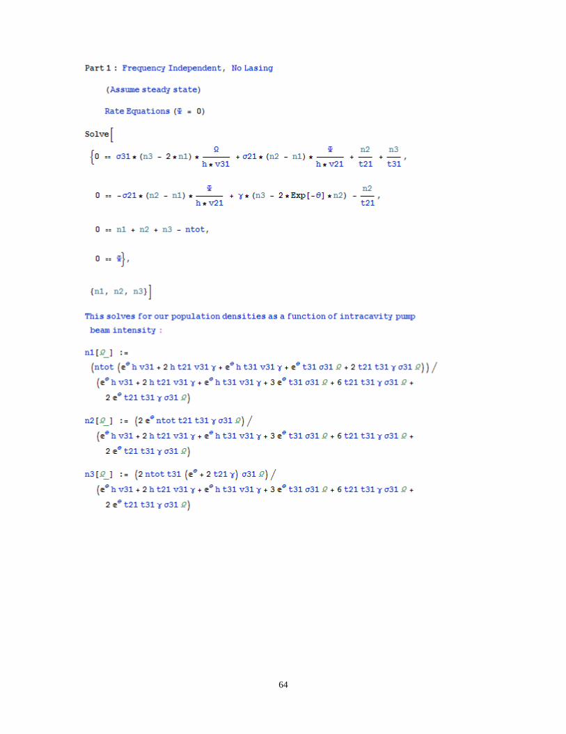
64

65

66

67

68

69

70

71

72

73

74

75

76

77
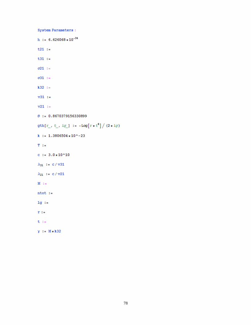
78

79

80
Bibliography 1. ChemGlobe, 2000. <http://www.chemglobe.org/> 2. Hager, G.D., and G.P. Perram, “A three-level analytic model for alkali metal vapor lasers: part I. Narrowband optical pumping,” Applied Physics B, (2010)
DOI 10.1007/s00340-010-4050-6. 3. Hager, G.D., and G.P. Perram, “A three-level analytic model for alkali metal vapor lasers: part II. Solutions for Broad Band Optical Pumping,” Applied Physics B, (2010) DOI 10.1007/s00340-010-4050-6. 4. Hecht, Jeff. “Back to the drawing board with Missile Beating Laser.” New Scientist. 22 Feb. 2010 <http://www.newscientist.com>. 5. J. E. Sansonetti, J. Phys. Chem. Ref. Data 35, 301–421 (2006); Erratum: 37, 1183 (2008) DOI:10.1063/1.2035727 . 6. Krupke, W.F. Diode-pumped alkali laser, US Patent 6,643,311, 2003. 7. Krupke, William. “Diode-pumped alkali lasers aim for single-aperture power scaling” SPIE Newsroom. 2008. 8. Perschbacher et al. “High Efficiency Diode Pumped Rubidium Laser: Experimental Results.” XVI International Symposium on Gas Flow and Chemical Lasers and High Power Laser Conference, Gmuden, Austria 29 January 2007. 9. Perram, Glen. “A New Approach for Tactical Laser Weapons: the Diode Pumped Alkali Laser.” AFIT/ENP 2011.
10. Pitz, Greg et al. “Pressure Broadening of the D1 and D2 lines in Diode Pumped Alkali Laser.” Proceedings of SPIE Vol. 7005 2008.
11. Pitz, G.A., C.V. Sulham, P. Jones, E.A. Acosta, and G.P. Perram, “ Accepted: AIAA Plasmadynamics and Lasers Conference (2010).
12. Rodriguez, Mary. “Go With the Flow: Novel Diode-Pumped Alkali Laser Achieves First Light.” Air Force Print News. 17 Dec. 2010 <http://www.wpafb.af.mil/news>. 13. Steck, Daniel. “Rubidium 87 D Line Data,” available online at http://steck.us/alkalidata (revision 2.1.4, 23 December 2010).

81
14. Sulham et al. “A pulsed, optically pumped rubidium laser at high pump Intensity.” Optics Communications, (2008). 15. Sulham, Cliff. “Laser Demonstration and Performance Characterization of Optically Pumped Alkali Laser System” AFIT Dissertation (2010). 16. Zameroski, N.D. et al. “A study of collisional quenching and radiation trapping kinetics for Rb(5p) in the presence of methane and ethane using time-resolved fluorescence.”Journal of Physics B (2009) DOI 10.1088/0953- 4075/42/24/245401.
17 Zweiback et al. “28W average power hydrocarbon-free rubidium diode pumped alkali laser.” Optics Express (2010).

82
REPORT DOCUMENTATION PAGE Form Approved OMB No. 074-0188
The public reporting burden for this collection of information is estimated to average 1 hour per response, including the time for reviewing instructions, searching existing data sources, gathering and maintaining the data needed, and completing and reviewing the collection of information. Send comments regarding this burden estimate or any other aspect of the collection of information, including suggestions for reducing this burden to Department of Defense, Washington Headquarters Services, Directorate for Information Operations and Reports (0704-0188), 1215 Jefferson Davis Highway, Suite 1204, Arlington, VA 22202-4302. Respondents should be aware that notwithstanding any other provision of law, no person shall be subject to an penalty for failing to comply with a collection of information if it does not display a currently valid OMB control number. PLEASE DO NOT RETURN YOUR FORM TO THE ABOVE ADDRESS. 1. REPORT DATE (DD-MM-YYYY) 24-03-2011
2. REPORT TYPE Master’s Thesis
3. DATES COVERED (From – To) June 2008 – Mar 2011
4. TITLE AND SUBTITLE Broadband Pumping Effects on the Diode Pumped Alkali Laser
5a. CONTRACT NUMBER
5b. GRANT NUMBER 5c. PROGRAM ELEMENT NUMBER
6. AUTHOR(S) Paul Jones, Civilian
5d. PROJECT NUMBER 5e. TASK NUMBER
5f. WORK UNIT NUMBER
7. PERFORMING ORGANIZATION NAMES(S) AND ADDRESS(S) Air Force Institute of Technology Graduate School of Engineering and Management (AFIT/EN) 2950 Hobson Way WPAFB OH 45433-7765
8. PERFORMING ORGANIZATION REPORT NUMBER AFIT/GAP/ENP/11-M04
9. SPONSORING/MONITORING AGENCY NAME(S) AND ADDRESS(ES) Brittany Edwards Southwestern Ohio Council for Higher Education 3155 Research Blvd., Suite 204 Dayton, OH 45420-4015
10. SPONSOR/MONITOR’S ACRONYM(S) SOCHE 11. SPONSOR/MONITOR’S REPORT NUMBER(S)
12. DISTRIBUTION/AVAILABILITY STATEMENT APPROVED FOR PUBLIC RELEASE; DISTRIBUTION UNLIMITED 13. SUPPLEMENTARY NOTES 14. ABSTRACT This research seeks to gain greater insight on the mechanics of The Diode Pumped Alkali Laser through analytic modeling techniques. This work is an extension to a previous model developed by Dr. Gordon Hager, and focuses on the addition of pump-beam bandwidth. Specifically, it seeks to determine the effect that broadband pumping has on laser performance. The model incorporates all the fundamental parameters within the laser system, including alkali concentrations, collision partner concentrations, pump bandwidth, length and temperature of gain medium, transmission, and reflectivity. Baseline operating conditions set Rubidium (Rb) concentrations ranging from 1012 - 1014 atoms/cm3, corresponding to operating temperatures ranging from 50 – 150 C. Ethane or Methane concentrations are varied corresponding to partial pressures from 100 – 500 Torr. The system is evaluated for incident beam intensity ranging from 0 – 30000 W/cm2, for both lasing and non-lasing system analysis. Output laser beam intensities scale well with input beam intensity and the model predicts optical to optical efficiencies of over 70%. 15. SUBJECT TERMS Diode Pumped Alkali Laser, gas laser, modeling, simulation, assessment tool
16. SECURITY CLASSIFICATION OF:
17. LIMITATION OF ABSTRACT UU
18. NUMBER OF PAGES 95
19a. NAME OF RESPONSIBLE PERSON Glen Perram, Ph.D. (AFIT/ENP)
a. REPORT
U
b. ABSTRACT
U
c. THIS PAGE
U
19b. TELEPHONE NUMBER (Include area code) 937-255-3636 x4504
Standard Form 298 (Rev. 8-98) Prescribed by ANSI Std. Z39-18


![Guide to Conducting Pumping Tests - B.C. … 4 ] HOW IS PUMPING RATE SELECTED? The well should be pumped at or above the intended pumping rate of the well and the well should not be](https://static.fdocuments.net/doc/165x107/5ccd45bc88c993de558dee0c/guide-to-conducting-pumping-tests-bc-4-how-is-pumping-rate-selected-the-well.jpg)


![Narrow-line fiber-coupled modules for DPAL pumping - … · Narrow-line fiber-coupled modules for DPAL pumping ... the diode-pumped alkali metal vapor laser (DPAL) [1] ... DPAL and](https://static.fdocuments.net/doc/165x107/5aff846b7f8b9af1148b59ed/narrow-line-fiber-coupled-modules-for-dpal-pumping-fiber-coupled-modules-for.jpg)


![Progress of on-chip wavelength stabilization of laser ... · diode-pumped Alkali laser (DPAL) [2]. A major advantage versus wavelength stabilization performed by a](https://static.fdocuments.net/doc/165x107/5aff846b7f8b9af1148b5a02/progress-of-on-chip-wavelength-stabilization-of-laser-alkali-laser-dpal-2.jpg)