1

Bid-Ask Spreads Around

Earnings Announcements

by

Daniella Acker

Mathew Stalker

and

Ian Tonks

Department of Economics,University of Bristol8, Woodland Road,Bristol BS8 1TN

January 18, 2001

Correspondence to:Daniella Acker 0117 928 8438e-mail: daniella.acker@bristol.ac.uk

We thank Ray Ball, Brad Cornell and participants at the European Finance AssociationAugust 2000 conference for helpful comments on this paper.

This work has arisen out of ESRC grant R000222682. We are grateful for this financialsupport.

2

Bid-Ask Spreads Around

Earnings Announcements

Abstract

This paper examines the determinants of bid-ask spreads and theirbehaviour around corporate earning announcement dates, for asample of UK firms over the period 1986-94. The paper finds thatclosing daily spreads are affected by order processing costs(proxied by trading volumes), inventory control costs (tradingvolumes and return variability) and asymmetric information(unusually high trading volumes). Spreads start to narrow 15 daysbefore an earnings announcement, and narrow further by the end ofthe announcement day. We also identify a puzzling phenomenon.There is only a ‘sluggish’ recovery of spreads after theannouncement: spreads continue to remain at relatively narrowlevels, and take up to 90 days to recover to their pre-announcementwidth.

JEL codes: M4, G1

3

I Introduction

This paper provides an empirical investigation of the movement in bid-ask spreads around

corporate earning announcements for a sample of UK firms over the period 1986-94. The

primary motivation for the study lies in the arguments put forward in the main market

microstructure theories of the spread and the implications they have for empirical testing.

The two principal theories of the bid-ask spread are represented by ‘asymmetric information’

models and ‘inventory control’ models. These are described in detail in section II with

appropriate references to the literature, but it is useful to summarise them here. The

asymmetric information models argue that the bid-ask spread compensates market makers for

adverse selection risk, the risk of trading with an investor who has superior information. The

emphasis of the inventory control models is on the costs of holding inventory. One of these is

the risk that the market maker finds himself holding non-optimal inventory levels and is unable

to adjust them by trading1. Both of these risks are related to trading volumes, but in opposite

directions. If investors obtain superior information, they are likely to trade on that

information, so that if market makers notice unusually high volumes of trade they will increase

their spreads to compensate them for the perceived adverse selection risk. Conversely, if

trading volumes are generally low, market makers will find it difficult to adjust their inventory

levels and will increase their spreads to compensate.

These arguments suggest that, to some extent, the level of asymmetric information in the

market and the risk of holding non-optimal inventory levels can both be proxied by some

measure of trading volume, which is the approach taken by many studies in this area (see Lee,

Mucklow and Ready (1993) and Stoll (1989), for example). However, it is clear that realised

volumes may not completely reflect the extent of adverse selection risk caused by information

asymmetry, or the risk of holding non-optimal stock levels caused by market illiquidity. This

is particularly the case in the period around earnings announcements.

Since earnings announcements convey new information to the stock market, an impending

announcement has the potential to induce information asymmetry by making private

1Inventory control risk also includes the risk that prices change while stocks are being held.

4

information acquisition attractive to potential traders2. Although market-makers will be

aware of the high level of information asymmetry present in the market, it is likely that the

asymmetry will not be entirely reflected in increased trades, for reasons such as legal

prohibitions on trading or general uncertainty. The spread will therefore be affected by an

increase in perceived adverse selection risk that is not reflected by an observable increase in

volumes.

Turning to inventory control, the risk of holding non-optimal inventory levels is related to the

depth of the market, that is the extent to which large trades can be undertaken at will, without

incurring large transactions costs (including significant price movements). Although this is

related to the volume of trades that are actually undertaken, the two are not identical, as

market depth depends on the ‘latent’ demand and supply of the stock. As shown in Lee et al

(1993), market depth narrows just before earnings announcements, increasing the extent of

unobservable inventory control risk. In this case, the spread will again be affected by an

increase in risk that is not reflected by an observable decrease in volumes.

It is likely, therefore, that the trading volume proxies commonly used in the literature to

analyse these determinants of the spread will not perform as well during announcement

periods as at other times. The aim of this paper is to test whether the fact that an

announcement is made carries incremental information in explaining the spread, over and

above the standard trading volume proxies (also controlling for other relevant variables).

We begin by examining the data to identify the patterns in spreads around earnings

announcement dates, allowing our choice of event period to be driven by the patterns

observed in the data. We then expand the simple univariate approach to control for

interactions of the spread with other market variables used in the literature, such as the

trading volumes discussed above, to investigate whether these variables explain movements in

the spread around announcement dates.

2There is a vast literature on the degree of information conveyed by earnings announcements, based on theseminal papers of Ball and Brown (1968) and Beaver (1968) (see the review articles by Strong (1992) andYadav (1992) for a summary). Although it has been found that prices anticipate information appearing inearnings reports and that there is often at least some post-announcement drift, the general consensus is thatearnings announcements do contain new information which is relevant to stock prices (Ball and Kothari(1994)).

5

In common with other studies we find that important determinants of bid-ask spreads are

trading volumes and return variability (see footnote 1). As predicted by the inventory control

model, volumes are negatively related to spreads, while return variability is positively

associated with spreads. We also find that unusually high trading volumes, proxying

asymmetric information as discussed above, are significantly positively related to the size of

the spread, as predicted by the adverse selection models.

As expected, spreads fall at the end of an announcement day, and volumes and return

variability are higher on that day. However, the fall in spreads appears to begin about three

weeks before the announcement, which is clearly at odds with the idea that adverse selection

risk and inventory control risk should cause spreads to widen before an announcement, and is

not consistent with studies based on US data, such as Lee et al (1993) and Yohn (1998).

Although an earnings announcement does appear to affect the spread over and above the

effect of the changes in the other variables at that time, the effect is to reduce it, rather than

increase it, as would be suggested by the arguments outlined above. A second puzzling

phenomenon is that after the release of earnings information, spreads not only fall, but remain

at the new lower level for up to 90 days after the announcement date.

The remainder of the paper is organised as follows. Section II reviews the previous literature

and section III describes the data. The methodology is outlined in section IV, while section V

presents the results. Section VI concludes the paper.

II Previous Literature

II(1) Models of the Bid-Ask Spread

There are two main theories of the bid-ask spread, ‘asymmetric information’ models and

‘inventory control’ models. In addition, empirical work by Roll (1984) and Stoll (1989) has

identified order processing costs as a component of the spread not dealt with by the two main

strands of the theoretical literature. We deal with each of these aspects of the spread in the

following paragraphs.

In the ‘asymmetric information’ models, dealers trade with liquidity traders and with informed

traders. The latter group has information which is superior to that of the dealers, so bid and

6

ask prices are set in order to compensate dealers for the perceived adverse selection risk. As

argued in Kyle (1985), Glosten and Milgrom (1985) and Easley and O’Hara (1987), if market

conditions are such that market makers3 become concerned that there is a higher proportion

of informed traders in the market, or that the informed traders have better information, they

will widen the bid-ask spread to compensate themselves for the additional adverse selection

risk. Therefore the “bid-ask spread can be a purely informational phenomenon, occurring

even when all the specialist’s fixed and variable transactions costs (including his time,

inventory costs, etc.) are zero.” (Glosten and Milgrom (1985) p72.)

In addition, Kyle (1985), Easley and O’Hara (1992) both predict that trading volumes will rise

when there is information asymmetry. This suggests a positive relationship between spreads

and unusually high trading volumes, since dealers interpret an unusually high volume as a sign

of an increased number of informed traders and widen their spreads accordingly.

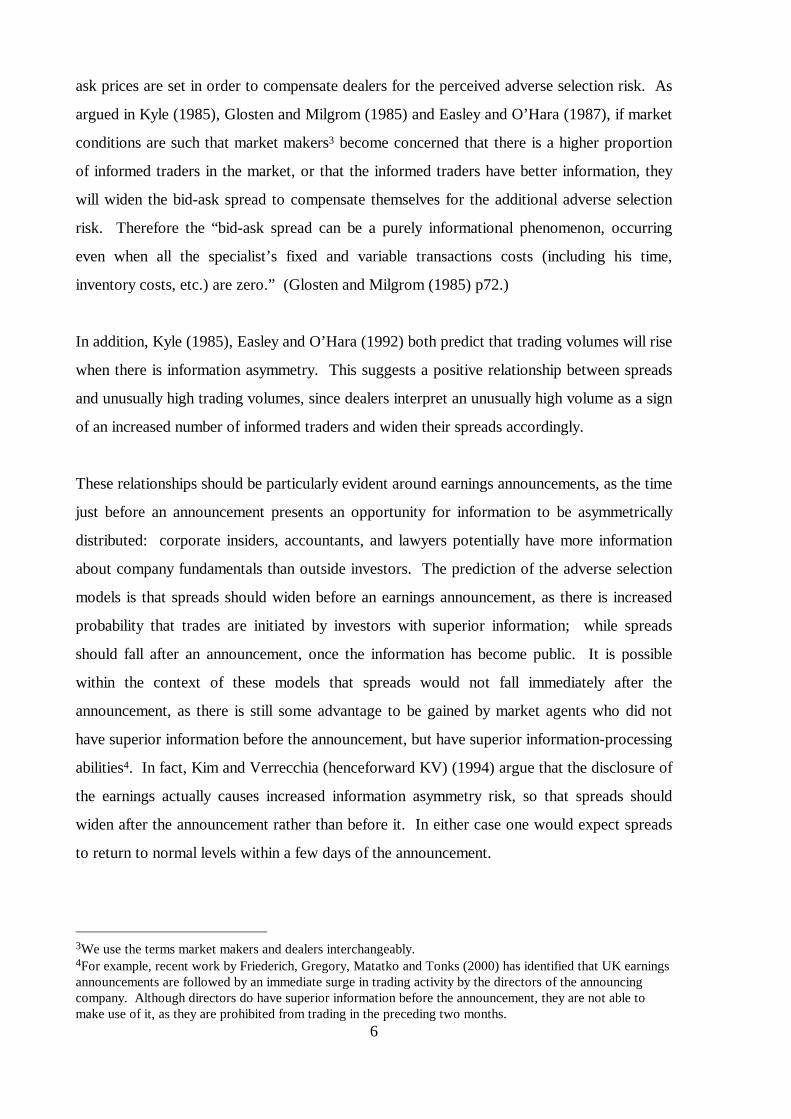
These relationships should be particularly evident around earnings announcements, as the time

just before an announcement presents an opportunity for information to be asymmetrically

distributed: corporate insiders, accountants, and lawyers potentially have more information

about company fundamentals than outside investors. The prediction of the adverse selection

models is that spreads should widen before an earnings announcement, as there is increased

probability that trades are initiated by investors with superior information; while spreads

should fall after an announcement, once the information has become public. It is possible

within the context of these models that spreads would not fall immediately after the

announcement, as there is still some advantage to be gained by market agents who did not

have superior information before the announcement, but have superior information-processing

abilities4. In fact, Kim and Verrecchia (henceforward KV) (1994) argue that the disclosure of

the earnings actually causes increased information asymmetry risk, so that spreads should

widen after the announcement rather than before it. In either case one would expect spreads

to return to normal levels within a few days of the announcement.

3We use the terms market makers and dealers interchangeably.4For example, recent work by Friederich, Gregory, Matatko and Tonks (2000) has identified that UK earningsannouncements are followed by an immediate surge in trading activity by the directors of the announcingcompany. Although directors do have superior information before the announcement, they are not able tomake use of it, as they are prohibited from trading in the preceding two months.

7

KV (1991a, 1991b) also argue that heterogeneous beliefs around earnings announcements

induce market participants to trade. Therefore increased information asymmetry at

announcement dates should result in higher trading volumes as well as increased spreads, in

line with the predictions of Kyle (1985), Easley and O’Hara (1992).

‘Inventory control’ models of the spread suggest that risk averse market makers have a desired

inventory position. Maintaining this inventory position implies taking on the risk of adverse stock

price movements, and market makers charge investors the spread to compensate them for this risk.

There are two aspects to inventory risk: the risk of being unable to trade the stock and the

risk that prices will change while stocks are being held.

The first of these risks will be higher, the more difficult it is for the market maker to return to

his desired inventory level (Amihud and Mendelson (1980) and Ho and Stoll (1980)). A

dealer who has recently purchased a large quantity of stock may temporarily reduce both his

bid and his ask quotes; the former to ensure that he is not quoting the best bid, and will not

therefore purchase any additional stock, and the latter to attempt to ensure that he is quoting

the most competitive ask in order to induce potential purchasers to trade with him, and reduce

his costly inventories. In a liquid5 market characterised by high trading volumes, the dealer

will only set a narrow ‘inventory spread’, since the dealer is assured of being able to quickly

restore an out-of-equilibrium position. The inventory control theories therefore predict that

as the liquidity of a stock increases, the compensation required by the market maker through

the spread is reduced, resulting in a negative relationship between trading volumes and

spreads.

The second feature of inventory risk is related to the underlying variability of the stock return.

Garber and Silber (1979), and Ho and Stoll (1981) demonstrate that the more volatile is the

stock price, the more the market maker is exposed to the risk of adverse price movements, and

consequently the wider is the bid-ask spread necessary to compensate the market maker, leading to

a positive correlation between return variability and the spread.

5 Kyle (1985) notes that the term market liquidity encompasses a number of transactional properties of markets, andwe use trading volumes as a measure of liquidity.

8

Finally, as with inventory risk, the existence of order processing costs will imply a negative

relationship between trading volumes and spreads. If dealers must recover fixed transaction

costs through the bid-ask spread, then the larger the number of transactions, the lower the

cost per transaction.

II(2) Evidence on Spreads Around Earnings Announcements

Using daily data on closing bid and ask prices Morse and Ushman (1983) were unable to

uncover any evidence that bid-ask spreads change around earnings announcements. It has

been suggested that this finding could be due to the information and volume effects working

in opposite directions, since the former causes spreads to widen, but the increased trading

volumes around the announcement dates result in a fall in spreads. Venkatesh and Chiang

(1986), also using daily data, found that spreads widened after earnings announcements only

when there was no other type of information released prior to the announcement date.

Lee, Mucklow and Ready (1993) used intraday data on bid and ask prices, and found that

spreads increased during the half-hour containing the earnings announcement, and remained

wider for the rest of that day. This increase in spreads continues for at least one trading day

after the announcement. They also reported a reduction in the quoted depth (the number of

shares available at each bid and ask price) prior to the time of the announcement. Yohn

(1998) also finds that spreads increase in the four days prior to an earnings announcement, on

the announcement day, and on the day after the announcement. He found that spreads revert

to their normal levels within ten days of the announcement.

Brooks (1996) looked at the change in the level of information asymmetry around earnings

and dividend announcements, using a regression-based measure of asymmetric information

due to Hasbrouck (1991). He also examined changes in the bid-ask spread. He found a

negative relationship between his measure of asymmetry and the bid-ask spread; also, his

results indicated little significant effect of announcements on either of the variables, although

there was weak evidence of a reduction in asymmetry before and after earnings

announcements. Using methods suggested by Roll (1984), Stoll (1989), George, Kaul and

Nimalendran (1991) for estimating the components of the spread, Krinsky and Lee (1996)

have analysed the components of the bid-ask spread around earnings announcements and

9

found that the adverse selection component (or information spread) increases markedly in the

period around the announcement.

III Data

The dataset which forms the basis for our empirical tests consists of a sample of 195 less-

liquid stocks on the London Stock Exchange. These stocks were all constituents of the FT-

All Share Index, and were in deciles two to four in terms of market capitalisation of those

constituents. Most of the companies in our sample were also constituents of the FT250 Midi

Index. The reason for focusing on this sample of less-liquid stocks is that spreads are much

wider than for the more liquid FTSE100 stocks, and therefore any movement in spreads

should be easier to identify. We collected earnings announcement data manually from a

sample of Extel cards for the period 1986-1992, and from the Extel Company Research CD-

Rom for the period 1992-94. This resulted in eight final earnings announcements per

company. The cards and news service record the date of each announcement. The timing of

the announcement of the earnings figure is at the discretion of the Stock Exchange, and

although the Exchange records the release time of the most recent earnings announcement for

a company, it proved impossible to obtain the exact time of past earnings announcements.

Trading volumes data were obtained from Datastream. We extracted turnover by volume

from Datastream datatype VO, which shows the number of shares traded per day. In addition

we also tested our results with a different definition of trading volume, Datastream datatype

AN, which is the aggregate number of shares transacted for non-stock exchange members.

These two series are highly correlated and the results did not alter with either definition. We

therefore only report results based on the VO definition of trading volume. All weekends and

public holidays were excluded from the sample, so that the maximum number of trading days’

data for any single company was 2,091.

Daily closing bid and ask prices were obtained from Datastream for all trading days between

27th October 1986 to 1st February 1994, a total of 2,091 trading days. These closing prices

are the best bid and ask prices quoted by market makers at the close of the market each day.

They are not ‘stale’ transactions prices, since quotes are updated even if no transactions take

place on that day, so there should be no concern about thin trading. Datastream does not

10

publish information on ask prices before 1986, and this therefore determined the starting date

for the sample.6

It is worth discussing whether using the Datastream daily closing prices is valid, when Lee et

al (1993) use intraday data. One argument that may be raised is that closing ‘best’ prices are

not indicative of ‘average’ market-maker behaviour during the day. The other possible

problem is that closing prices are, in general, not representative of intraday prices. We

address each of these issues below, first outlining the procedure for setting bid and ask prices

on the London Stock Exchange (LSE).

Over the period 1986-97 the LSE operated as a dealer market with competing market makers,

each market maker continuously quoting a bid price at which he was willing to buy securities,

and an ask price at he was willing to sell. Although its trading mechanism changed in 1997 to

an order-driven system for the most liquid FTSE100 stocks, over the time period 1986-94

which we examine, and for the FTSE250 stocks in our sample, the relevant trading

mechanism remains the quote-driven system. Trading in shares at the LSE takes place by

telephone through a small number of registered market makers. Market makers announce on

SEAQ screens firm prices at which they are willing to buy and sell given quantities of stock

up to a preset maximum. The lowest ask price and highest bid price, which represents the

best prices from the point of view of the customer, are highlighted on the SEAQ screens and

are called the ‘yellow strip’ prices or the ‘touch’.

The bid and ask prices of competing market makers might differ, and the closing prices on

Datastream are the bid and ask prices at the touch, representing the best prices - the

narrowest spread - available. A rule of the Exchange is that brokers are obliged to trade on

behalf of their clients at the best prices, so that outside investors will always trade at the

touch. Indeed it is not obvious why market makers set prices at anything other than the

touch, since they will not generate any trade. Possible explanations involve issues of

inventory concerns, and the existence of differential information between market makers7.

Under both asymmetric information and inventory control theories of the spread, individual

market makers may set one of their quotes at a different level to the other market makers, so

6We use daily closing prices since intra-day stock price data from the London Stock Exchange is not widelyavailable prior to 1992, and our dataset on earnings announcements spans the years 1986-94.

11

they will be outside the touch on one side, and at the touch on the other. The subsequent

imbalance in order flow will cause the other market makers to adjust their quotes or suffer the

consequences of the imbalance. These are exactly the arguments tested in Hansch, Naik and

Viswanathan (1998), who examine the price setting behaviour of individual market makers on

the LSE. Board, Vila and Sutcliffe (1997) also examine market maker interactions on the

LSE and find that typically market makers maintain a constant individual bid-ask spread.

Importantly, when individual market makers change their quotes in such a way as to affect the

touch, this will usually move the mid-point of the touch in the same direction. This finding

justifies the generally accepted belief that changes in the touch are a good proxy for the

quote-setting behaviour of individual market makers.

Turning to the question of whether closing prices are representative of intraday prices,

Abhyankar, Ghosh, Levin and Limack (1997) examine intraday ‘inside’ spreads (spreads at

the touch) on the LSE and find that average spreads vary only slightly during the mandatory

quote period. This suggests that the average spread over the day should be an unbiased

predictor of the closing spread. In fact, we were able to test directly for bias, since we had

access to some intraday data provided by the LSE, relating to a small sub-sample of seven of

the companies in our sample8. The intraday dataset consists of a continuous record of all

transactions and the best ask and bid quotes in these seven stocks between 1st April 1992 and

11th March 1994, which represents 492 trading days. We were therefore able to use this data

to test the hypothesis that intraday spreads are an unbiased estimator of closing spreads.

Finally, as noted above, the study by Lee et al (1993) makes use of intraday stock price data,

and provides evidence on the movement in spreads at half-hourly intervals, although the

volatility of intraday data forces them to average the half-hourly stock price reaction for the

days before and after the earnings announcement, to obtain a clear picture of the effect of the

earnings announcement on spreads. Although using closing prices clearly restricts the

examination of the immediate effect of the earnings announcement on spreads, an advantage

of this data is that we were able to investigate the daily movement in spreads over every

trading day in 1986-94 (see footnote 6). This period includes 1,505 final earnings

announcements for the 195 companies, about eight announcements per company. Hence we

7 Market-microstructure models typically assume symmetric information between market makers.8We wish to thank John Board for providing this data, which was used in Board and Sutcliffe (1995).

12

are able to control for any time effects in the movements in spreads around earnings

announcements, which would not be possible in a short window of perhaps one year’s worth

of intraday data.

Table 1 presents descriptive statistics of daily closing spreads, daily trading volumes and daily

return variability.

TABLE 1 ABOUT HERE

Panel A shows that the average spread across all observations is 2.3%. The median is 1.84%,

indicating some right skewness in the distribution. The spread is bounded from below by zero

and the upper 10% of the observations are above 4.2%. Panel B shows that the overall

standard deviation is 0.0175%. The ‘within’ component, which reflects the contribution of

variation over time to the overall standard deviation, is of the same order of magnitude as the

‘between’ component, which reflects the contribution of cross-sectional variation.9

Mean daily trading volume is 603,300, considerably higher than the median of 153,600. In

addition, the overall standard deviation is extremely high and the distribution ranges from

6,000 at the lower end to 1.5 million at the upper end. The ‘between’ component of the

standard deviation is less than half the ‘within’ component, implying that the time series

variation is much greater than the cross-sectional variation. To avoid the distortion caused by

large outliers we transformed the trading volume variable by taking natural logarithms.

The average value of the squared daily return, which proxies return variability, is 3.774 %2.

More than 25% of the observations are zero, reflecting the fact that on a large number of days

no price change has occurred. From Panel B it can be seen that, as with the trading volumes,

the ‘within’ component of the standard deviation is more than ten times greater than the

‘between’ component, implying that the time series variation is much greater than the cross-

sectional variation.

9Panel A in table 1 shows that there are considerably fewer observations on daily trading volumes than ondaily spreads, because Datastream reports only sporadic trading volumes during 1987 and 1988.

13

In Panel C we report the mean values of daily spreads and volumes during the event window

(see below for a discussion on the choice of window). It can be seen that spreads start to fall

below their normal level 15 days before the announcement date. On the announcement date

spreads narrow to 2.16% on average. They stay down for a further two days, begin to rise

and only begin to approach the long-run norm in the (+16, +90) period. Trading volumes

increase dramatically on the day of the announcement and stay high on the following two

days.

These descriptive statistics are indicative of the relationship among spreads, trading volumes,

return variability and earnings announcements. However, they do not take account of the

interactions between these variables, which are examined in the models described in the

following section.

IV Methodology

In a preliminary investigation of the data we examined the movement in spreads over the

reporting year. We estimated equation (1), which assigns dummies to each five-day period

over the year, except for the announcement day, day 0.

, , ,A B Dj t j j ts t tt

= + + eå

(τ ∈{(-125, -121), (-120, -116), ... (-5, -1), (1, 5), (6, 10), ..., (121, 125)}) (1)

where sj,t is the bid-ask spread of company j at the close of trading on day t and is defined as

the difference between the ask and the bid prices as a percentage of the mid-point price:

sj,t = 2*(ASKj,t - BIDj,t)/(ASKj,t +BIDj,t);

Dj,τ is a set of dummies, which take the value 1 for each 5-day trading period, τ, around each

earnings announcement; and 0 elsewhere; and

εj,t is an error term

There are typically 250 trading days in an accounting year, and the classification of this set of

dummies ensures that every 5-day period in the 125 trading days either side of the

announcement is included in the regression. The periods τ ∈ {(-125, -121), (-120, -116), ...

(-5, -1), (1, 5), (6, 10), ..., (121, 125)} encapsulate the usual interval between each final

14

earnings announcement, as shown in Figure 1, where we present the frequency distribution of

the time interval between each company’s successive earnings announcements. For each

announcement this time interval is equally divided between a ‘pre-announcement’ period

(denoted by a minus sign) and a ‘post-announcement’ period (denoted by a plus sign), centred

around the day of the earnings announcement (day 0).

FIGURE 1 ABOUT HERE

All days outside the period (-125, +125) were dropped from the estimation, so the intercept

coefficient, A, is the estimated spread on the announcement day. In Figure 2 we present the

estimation results. The intercept is just above 2.3%, confirming the descriptive statistics in

Panel A of table 1. It can be also seen that spreads appear to decline from about 90 days

before the announcement, fall sharply on the day of the announcement, and stay down until

about 90 days after it.10,11 This is surprising in view of the results of Lee et al (1993) and

Yohn (1998), but more comprehensive tests resulted in the same pattern.

FIGURE 2 ABOUT HERE

We used this preliminary investigation of the spreads pattern over the year to determine the

length of the event period, choosing an event window running between day -90 and day +90.

Within this period we identified sub-intervals to reflect the patterns suggested by Figure 2.

These sub-intervals were as follows: (-90, -16), (-15, -3), -2, -1, 0, +1, +2, (+3, +15), (+16,

+90).

We then estimated two sets of regression equations to investigate the behaviour of spreads,

trading volumes and return variability around earnings announcements. The first set

(equations (2a), (2b) and (2c)) represents simple univariate tests designed to confirm the

pattern suggested by the descriptive statistics, namely that spreads, volumes and return

variability do indeed change during the chosen event window. This is done by assigning

10For some stocks the bid and ask prices are no more than a few pence, so discreteness of prices means thatpercentage spreads are extremely sensitive to price movements on either side of the spread. We re-estimatedequation (1) excluding observations with a mid-price below £1 and the results were not affected.11 It appears that there is a peak in spreads round about the time when announcements of interim earnings aremade. However, we estimated equation (1) including a dummy variable to identify interim announcementperiods, and it did not have a significant coefficient.

15

dummy variables to the sub-intervals within the event period and simply regressing the spread,

volume or return variability on these dummies:

, , ,j t T j T j tT

s a b D e= + +å (2a)

, , ,j t T j T j tT

Vol a b D e¢ ¢ ¢= + +å (2b)

, , ,j t T j T j tT

Var a b D e¢¢ ¢¢ ¢¢= + +å (2c)

where sj,t is the spread, as defined above;

Volj,t is the log of the total number of shares traded (buys and sells) in company j’s shares

during day t;

VARj,t is the square of stock j’s return on day t, a proxy for return variability12; and

Dj,T are dummy variables which now take on the value 1 if period T lies in the event window,

and 0 otherwise; T ∈ {(-90, -16), (-15, -3), -2, -1, 0, +1, +2, (+3, +15), (+16, +90)}.

The theoretical literature discussed in section II typically predicts a widening of the spread

before the announcement date, with a reversion to normal levels soon afterwards.

Conversely, the KV model predicts a widening of the spread and increase in volumes after the

announcement. Therefore positive coefficients on the T

b - in equation (2a) (where

T - indicates dates before the announcement) would support the conventional models of the

spread. In addition the coefficients on some or all of the bT+ and b0 (since prices are measured

at the close of trading) should not be significantly different from zero, depending on how long

it takes the market to adjust to the new information. The KV model will be supported if b0,

and some or all of the bT+ are significantly positive. The same arguments apply to the

′b coefficients in equation (2b).

Turning to equation (2c), the general finding in the literature is that volatility increases

immediately after an announcement (see Beaver (1968) and Kalay and Loewenstein (KL)

(1985) for early examples and Acker (1999) for a more recent one) and remains high for one

or two days. Some papers have also found that volatility is lower than usual in the period

12 We proxy stock return variability by the square of daily returns, as in Venkatesh and Chiang (1986) and Yohn(1998).

16

leading up to an announcement although not immediately before it (Beaver (1968) and KL

(1985) again; and two studies using implied volatilities, Donders and Vorst (1996) and Acker

(2000) also obtain this result). We would therefore certainly expect 0b¢¢, 1b¢¢ and possibly 2b¢¢

to be significantly positive; and some or all of the T

b -¢¢ may also be negative.

The second set of equations explicitly models the interactions between trading volumes,

return variability and spreads. We use a series of nested models to identify the extent to

which the spread can be explained by order processing costs (trading volumes), inventory

control costs (trading volumes and return variability) and asymmetric information (excess

volume). The models, shown in order of increasing complexity, are as follows:

Model 1 sj,t = α + βVolj,t + ζ j,t

Model 2 sj,t = α + βVolj,t + γ XVolj,t + λ VARj,t + φ MVARt + ξj,t

Model 3 , , , , , ,+ + j t j t j t j t t T j T j tT

s Vol XVol VAR MVAR D= a + b + g l f + d + Jå

where XVolj,t is the excess trading volume, defined as the percentage difference between firm

j’s actual trading volume and its average trading volume over time, when this difference

is positive; and zero otherwise;13

MVARt is the unweighted mean of VARj,t across all stocks on day t, which is a proxy for

market variability; and

ζ j,t, ξj,t, ϑj,t are error terms.

(Other variables are defined above)

Model 1 investigates the relationship between spreads and trading volumes, to identify the

extent to which movements in the spread are related to observable inventory control and

transactions costs considerations. As discussed above, the order processing costs and/or

inventory control should result in a negative relationship between the daily level of trading

volume and the size of the spread (β < 0).

Model 2 includes excess volumes and return variability measures as additional control

variables. Excess volume is used as a proxy for information asymmetry, as suggested by the

Kyle (1985), Easley and O’Hara (1992) and KV (1991a 199b) models. A positive

17

relationship between the excess trading volumes and spreads (γ > 0) confirms the joint

hypothesis that both spreads and excess volumes reflect observable information asymmetry.

The coefficients on the return variability terms, λ and φ, should be positive, reflecting the fact

that spreads will increase with inventory risk.

Having established the relationship between closing spreads, daily trading volumes and return

variability, we then investigate in more detail the change in spreads around earnings

announcements. Model 3 includes the sub-interval event period dummy variables (the ‘T

dummies’). The model examines whether there is any change in the spread in the event period

which is not accounted for by normal and excess trading volumes, or by return variability.

Significant coefficients on the dummies would suggest that the bid-ask spread during the

event window reflects changes in information asymmetry or costs which are not entirely

captured by the explanatory variables in Model 2.

We might anticipate that the distributions of the error terms in Models 1 to 3 (ζ j,t, ξj,t, ϑj,t) will

vary over the j companies. One solution to this problem is to correct the estimated standard

errors from the pooled regressions for heteroscedasticity. Our first set of results (table 3

below) therefore uses White’s heteroscedastic-consistent covariance estimator. A second

approach exploits the fact that we have panel data on a cross-section of firms over time, and

models the error terms appropriately. The residuals in models 1 to 3 (and also in equations

(2a) to (2c)) can be separated into two components, νj + ωjt, say, where νj is a firm-specific

residual, and ωjt has all the usual properties (zero mean, homoscedastic, uncorrelated with

itself and with νj). Assuming that the νj are fixed and estimable we may estimate the models

as fixed effects panel models, in which case the νj may be interpreted as dummy variables for

each firm, taking on the value of unity for firm j, and zero elsewhere. We therefore re-

estimated all models as fixed effects panel models, with results presented in table 4 below.

The results are discussed in the following section.

Finally, we re-estimated the models including dummy variables for calendar years, since the

size of the spread in bull and in bear markets is likely to vary considerably.

13Logs of volume were not used for excess volume, as this would leave zero excess volume undefined.

18

V Results

In table 2 we present the results of estimating equations (2a) to (2c). The results of the

pooled estimations are reported in the first two columns and those of the fixed effects

estimations are in the third and fourth columns. The high values of the F statistics in these

last two columns verify the joint significance of the fixed effects terms.

TABLE 2 ABOUT HERE

The equation (2a) results show that spreads do drop significantly by the end of the

announcement day, as predicted by the standard microstructure models, and in contrast to the

KV predictions. The size of the drop is of the order of 0.16 to 0.2 percentage points, which

reduces the spread to below normal levels, whereas the standard models predict that spreads

return to normal immediately after the announcement. Although the drop reaches its

maximum by the end of the announcement day, the reduction in spreads appears to start some

15 days before the announcement day. There is evidence from the fixed effects regression

that spreads in the period (-90, -16) increase very slightly, although this is not apparent in the

pooled model. After the announcement both models indicate that spreads begin to rise again,

although they stay below their ‘normal’ level of 2.3% for the next 90 days.14

The equation (2b) regressions are concerned with trading volumes. As expected, volumes

reach a maximum on day 0. The volume increase begins on day -1 and continues for 15 days

after the announcement, although, as with the spreads, the maximum increase is on the

announcement day. The implications of the regressions for the (-90, -2) and (+16, +90)

periods are ambiguous. The pooled and fixed effects models generate different results,

although the general pattern appears to be that there are higher volumes than normal during

these periods.

The equation (2c) results show that, as expected, there is a substantial increase in volatility on

the day of the earnings announcement, which continues into the following day, although at a

reduced level. Interestingly, in line with the papers mentioned above, we also find a dip in

14Earlier regressions which were based on a longer post-announcement event period indicated that coefficientson post-90 day dummies were not significantly different from zero at conventional levels.

19

volatility in the ninety day period leading up to the announcement, although not immediately

before it. There is also a dip in the ninety day period after the announcement, and this result

is consistent with the findings in Acker (2000).

In summary, it is clear that volumes, spreads and return variability are affected by the

announcement, with generally lower spreads and higher volumes in the period surrounding the

announcement; and high variability on the announcement day and the day after.

Tables 3 and 4 present the results of the pooled and panel regressions respectively, fitting

models 1 to 3, together with the expanded model 3 which includes the calendar year

dummies. Model 1 shows that, as expected, the relationship between the spread and trading

volume is significantly negative, reflecting the reduction in the fixed costs as the number of

trades increases. The effect is less pronounced in the panel regressions, suggesting that

including firm-specific dummies soaks up much of the volume effect: market-makers may

well keep to historically-determined spreads according to the company being traded, the

spread being highly correlated with the historical trading volumes in that company.

TABLES 3 AND 4 ABOUT HERE

Model 2 includes trading volumes, excess volumes, and firm and market return variability as

explanatory variables. The previous results are robust to amending the model specification,

again showing a highly significant negative relationship between spreads and normal trading

volumes. As predicted, spreads are positively related to excess volumes, and to firm and

market return variability. Again the pooled and the panel results are very similar.

Model 3 examines the effects of an announcement on the spread, while controlling for the

effects of changes in volumes, excess volumes and variability at this time. The results in

tables 3 and 4 for model 3 show that the ‘normal’ relationships established between spreads,

volumes, excess volumes and variability in model 2 are robust to the inclusion of the T

dummy variables.

The fixed effects regressions reveal that the T dummies are all negative and most are

significant at conventional levels. In the pooled regression, these dummies are also negative,

20

although not all are significant at conventional levels. Clearly the addition of the fixed effects

terms refines the specification of model 3. Both the fixed effects and the pooled regressions

have a significantly negative coefficient on the day 0 dummy. This demonstrates that spreads

narrow significantly by the end of the announcement day, even after having accounted for the

effects of higher trading volumes and additional return variability.

These results suggest that, having controlled for the effects of changes in the various

independent variables, spreads fall significantly on the announcement day. In fact, they

narrow from 15 days before the announcement and continue to fall on and after the

announcement day. Surprisingly they do not revert to normal levels until more than 90 days

after the announcement.

We argued in Section II that the period preceding the announcement is likely to be

characterised by an unusual amount of asymmetric information, which should be eliminated

once the announcement has been made. Our results confirm that the degree of asymmetric

information is reduced by the end of the announcement day, but the fact that spreads start to

fall quite some time before the announcement is not explained by the theoretical models.

Neither is the sluggish recovery of spreads to their pre-announcement levels.

Finally we return to the issue discussed in the data section, namely the validity of using

closing daily spreads rather than intraday spreads. Using the sub-sample of seven stocks for

which we have intraday data, we test whether the mean daily spread is an unbiased predictor

of the closing spread by estimating the following equation:

sj,t = κ + ρ s j t, +ηj,t (3)

where

sj,t is the closing bid-ask spread for day t of company j, as defined above; and

s j t, is the average bid-ask spread over day t of company j. This average is computed by

observing the registered spread at the touch each time a transaction takes place

during the day, and calculating the mean spread during that day.

21

The null hypothesis of unbiasedness in spreads is that κ = 0 and ρ = 1. The results are

presented in table 5. Column 1 of the table shows that, as predicted, the intercept coefficient

is not significantly different from 0 and the slope coefficient is not significantly different from

1. Column 2 shows the results of estimating an expanded model which includes the T

dummies referred to earlier. This second model allows for the possibility that the relationship

between spreads throughout the day and closing spreads changes during the event window.

Again the intercept and slope coefficients are as expected, but the coefficient on the

announcement day dummy is significantly positive. This implies that on the day of an earnings

announcement spreads are wider at the end of the day than they are, on average, during the

day. These results strengthen our earlier conclusions. The narrowing of the spreads observed

at the close of the announcement day and reported in tables 2 to 4 must underestimate the

general narrowing that occurs during the day.

VI Conclusions

In this paper we have investigated the behaviour of bid-ask spreads around earnings

announcements. We find that spreads fall, and volumes and return variability rise on

announcement days. In addition, spreads are affected by normal and excess trading volumes

and by return variability. These findings are consistent with both asymmetric information and

inventory control models of the bid-ask spread.

We have examined whether spreads change significantly around earnings announcements, on

the basis that this is a time when one would expect unobservable information asymmetries to

be most pronounced. After allowing for the higher trading volumes and variability on the

announcement day, spreads narrow by the end of the day of the earnings announcement.

These results were true in both our pooled regressions and in the fixed effects models. The

strong conclusion that we draw from our empirical work is that market makers quote

narrower spreads once the earnings have been announced. This result is in contrast to the

findings of Lee et al (1993) and Yohn (1998) who report that for US data spreads rise before

the earnings announcement and remain at a higher level even after the announcement has been

made.

A puzzling characteristic of our data set is the apparent extended effect of the announcement.

The narrowing of spreads and the increase of trading volumes begins at least fifteen days

22

before the announcement date. Even more surprising is the sluggish recovery of both spreads

and volumes. Spreads remain below normal levels for up to 90 days after the announcement;

similarly, volumes are abnormally high during this period.

23

Figure 1 Distribution of number of trading days between successive earningsannouncements 1986 - 1994

Number of trading days before (-) or after (+) announcement

0

200

400

600

800

1000

1200

-200 -175 -150 -125 -100 -75 -50 -25 0 25 50 75 100 125 150 175 200

Frequency

The figure shows the frequency distribution of the time interval between each company’s successive earningsannouncements. For each announcement this time interval is equally divided between a ‘pre-announcement’period (denoted by a minus sign) and a ‘post-announcement’ period (denoted by a plus sign), centred aroundthe day of the earnings announcement (day 0).

24

Figure 2 Estimated spreads around announcement dates

Trading days before (-) or after (+) announcement

0.02

0.021

0.022

0.023

0.024

0.025

0.026

-125 -100 -75 -50 -25 0 25 50 75 100 125

- - - 95% confidence intervals

Estimated spread___

%

The figure shows the estimated spread over the reporting year, together with 95% confidence intervals for thespread. The estimates were generated using equation (1): , , ,A B Dj t j j ts t t

t

= + + eå

25

Table 1 Descriptive Statistics

Panel A: Distribution of spread, trading volume and return variability

PercentilesNumber of

observationsMean 10% 25% Median 75% 90%

Daily spread 402,729 0.0230 0.0086 0.0123 0.0184 0.0278 0.0420Daily trading volume(000) 282,306 603.3 6.0 29.9 153.6 578.8 1,548.0Ln (volume) 282,074 4.7876 1.7917 3.4012 5.0370 6.3620 7.3454Daily variability ofcompany returns(%2)

402,244 3.774 0.000 0.000 0.279 1.793 6.805

Panel B: Standard deviations of spread, trading volume and return variability

Overall standarddeviation

Between Within

Daily spread 0.0175 0.0110 0.0137Daily trading volume(000) 1,773,331 744,640 1,604,475Ln (volume) 2.1182 1.4625 1.5670Daily variability ofcompany returns (%2) 24.406 2.415 24.289

‘Between’ denotes the cross-sectional standard deviation of the time series means‘Within’ denotes the cross-sectional mean of the time series standard deviations

Panel C: Mean values of spreads and trading volumes around earnings announcement

Days aroundannouncement

Daily spread Daily trading volume(000)

Ln(volume)

(-90,-16) 0.0235 593.98 4.779(-15,-3) 0.0225 533.65 4.739-2 0.0222 609.63 4.875-1 0.0223 595.74 4.9670 0.0216 1,843.98 6.250+1 0.0215 1,196.94 5.908+2 0.0216 780.42 5.371(+3,+15) 0.0219 644.17 4.974(+16,+90) 0.0221 588.75 4.757

Spreads and trading volumes were averaged across companies for the following sub-intervals around theearnings announcements: (-90, -16), (-15, -3), -2, -1, 0, +1, +2, (+3, +15), (+16, +90).

26

Table 2 Estimates of equations (2a) to (2c)

Pooled Fixed EffectsEquation (2a)

(dependentvariable:spreads)

Equation (2b)(dependent

variable: logvolumes)

Equation (2c)(dependent

variable: dailyreturn

variability %2)

Equation (2a)(dependentvariable:spreads)

Equation (2b)(dependent

variable: logvolumes)

Equation (2c)(dependent

variable: dailyreturn

variability %2)

Constant 0.0236 4.7600 4.192 0.0233 4.7250 4.139(498.537)** (691.386)** (60.249)** (621.255)** (922.552)** (62.355)**

DUM(-90, -16) -0.0001 0.0201 -0.539 0.0003 0.0673 -0.045(-1.760) (1.937)* (-5.138)** (5.192)** (8.734)** (-4.528)**

DUM(-15, -3) -0.0011 -0.0200 -1.063 -0.0006 0.0242 -0.989(-7.967)** (-1.034) (-7.492)** (-6.100)** (1.689) (-5.285)**

DUM-2 -0.0014 0.1156 1.205 -0.0009 0.1707 1.281(-2.981)* (1.775) (0.680) (-2.582)* (3.547)** (2.023)*

DUM-1 -0.0013 0.2075 -0.230 -0.0008 0.2502 -0.155(-2.758)* (3.171)* (-0.621) (-2.279)* (5.177)** (-0.244)

DUM0 -0.0020 1.4902 22.166 -0.0016 1.5810 22.239(-4.359)** (23.126)** (11.538)** (-4.358)** (33.219)** (35.057)**

DUM+1 -0.0021 1.1479 4.029 -0.0017 1.2375 4.098(-4.616)** (17.807)** ( 4.658)** (-4.666)** (25.990)** (6.482)**

DUM+2 -0.0019 0.6111 -0.103 -0.0015 0.7015 -0.000(-4.269)** (9.475)** (-0.217) (-4.275)** (14.726)** (-0.058)

DUM(+3, +15) -0.0017 0.2141 -0.835 -0.0013 0.2839 -0.766(-12.871)** (11.155)** (-5.241)** (-12.295)** (19.987)** (-4.096)**

DUM(+16,+90)

-0.0015 -0.0024 -1.017 -0.0010 0.0514 -0.094

(-20.878)** (-0.232) (-11.025)** (-18.533)** (6.801)** (-9.487)**

R squared 0.0016 0.0038 0.0036F(194, 402525) 1287.31**F(193, 281871) 1219.5**F(194, 402040) 20.04**No. in sample 402,729 282,074 402,244 402,729 282,074 402,244

1. The table shows the regression results on equations (2a) to (2c):

, , ,j t T j T j tT

s a b D e= + +å (2a)

, , ,j t T j T j tT

Vol a b D e¢ ¢ ¢= + +å (2b)

, , ,j t T j T j tT

Var a b D e¢¢ ¢¢ ¢¢= + +å (2c)

where sj,t is the bid-ask spread of company j at the close of trading on day t and is defined as the

difference between the ask and the bid prices as a percentage of the mid-point price;

Volj,t is the log of the total number of shares traded in company j’s shares during day t;

VARj,t is the square of stock j’s return on day t, a proxy for return variability; and

Dj,T are dummy variables which take on the value 1 if period T lies in the event window, and 0

otherwise; and T = {(-90, -16), (-15, -3), -2, -1, 0, +1, +2, (+3, +15), (+16, +90)}.

2. t-statistics in parentheses; * = significant at 5%; ** = significant at 1%.

27

3. F(., n) is an F-test on the joint significance of the fixed effect terms, where . is the number of companies

and n is degrees of freedom. (No R-squared is given in this table as it is not defined in a fixed effects

model)

28

Table 3: Models 1 to 3 (pooled)

Model 1 Model 2 Model 3 Model 3 with year dummies

Constant 0.0317 0.0313 0.0317 0.0275(344.294)** (296.633)** (277.217)** (220.933)**

Volj,t -0.0017 -0.0019 -0.0019 -0.0018(-102.030)** (-93.585)** (-93.852)** (-92.850)**

XVolj,t 0.0004 0.0004 0.0004(9.478)** (9.451)** (9.589)**

VAR j,t 0.8108 0.8119 0.8066(9.240)** (9.196)** (9.303)**

MVARt 3.0707 3.0343 1.0589(23.452)** (23.175)** (8.629)**

DUM(-90, -16) 0.0000 -0.0005(0.381) (-5.376)**

DUM(-15, -3) -0.0008 -0.0011(-4.573)** (-6.794)**

DUM-2 -0.0009 -0.0012(-1.546) (-2.085)*

DUM-1 -0.0004 -0.0008(-0.845) (-1.621)

DUM0 -0.0017 -0.0020(-3.227)** (-3.911)**

DUM+1 -0.0004 -0.0008(-0.820) (-1.657)

DUM+2 -0.0006 -0.0009(-1.143) (-1.952)

DUM(+3, +15) -0.0009 -0.0013(-6.174)** (-8.744)**

DUM(+16, +90) -0.0011 -0.0014(-13.401)** (-17.217)**

DUM90 0.0060(60.204)**

DUM91 0.0070(64.126)**

DUM92 0.0102(82.505)**

DUM93 0.0048(48.746)**

DUM94 0.0016(18.205)**

DUM95 0.0025(9.940)**

R squared 0.0372 0.0609 0.0618 0.0935No. in sample 281,553 281,529 281,529 281,529

1. The table shows the regression results onModel 1 sj,t = α + βVolj,t + ζ j,tModel 2 sj,t = α + βVolj,t + γ XVolj,t + λ VARj,t + φ MVARt + ξj,tModel 3 , , , , , ,+ + j t j t j t j t t T j T j t

T

s Vol XVol VAR MVAR D= a + b + g l f + d + Jåwhere XVolj,t is excess trading volume;VARj,t is the square of stock j’s return on day t, and MVARt is the unweighted mean of VARj,t across allstocks on day t.

2. t-statistics in parentheses (based on White’s heteroscedastic-consistent covariance estimator); * = significant at 5%; ** = significant at 1%

29

Table 4 Models 1 to 3 (fixed effects)

Model 1 Model 2 Model 3 Model 3 with year dummies

Constant 0.0261 0.0256 0.0259 0.0213(321.081)** (299.639)** (281.371)** (201.772)**

Volj,t -0.0005 -0.0007 -0.0007 -0.0006(-30.536)** (-39.380)** (-38.625)** (-33.560)**

XVolj,t 0.0001 0.0001 0.0001(8.205)** (8.202)** (8.388)**

VAR j,t 0.4612 0.4633 0.4554(44.201)** (44.344)** (45.117)**

MVARt 3.2586 3.2200 1.1314(55.197)** (54.556)** (19.089)**

DUM(-90, -16) 0.0003 -0.0003(3.969)** (-4..098)**

DUM(-15 ,-3) -0.0005 -0.0009(-4.354)** (-7.522)**

DUM-2 -0.0008 -0.0011(-1.877) (-2.687)**

DUM-1 -0.0005 -0.0009(-1.200) (-2.266)*

DUM0 -0.0020 -0.0025(-4.993)** (-6.247)**

DUM+1 -0.0013 -0.0017(-3.136)** (-4.436)**

DUM+2 -0.0011 -0.0016(-2.797)** (-3.977)**

DUM(+3, +15) -0.0010 -0.0014(-8.683)** (-12.228)**

DUM(+16,+90) -0.0010 -0.0013(-15.025)** (-20.491)**

DUM90 0.0065(76.077)**

DUM91 0.0074(88.834)**

DUM92 0.0107(122.659)**

DUM93 0.0045(53.682)**

DUM94 0.0016(19.123)**

DUM95 0.0029(13.492)**

F(193, 281358) 1,124.23F(193, 281331) 1,115.16F(193, 281322) 1,117.03F(193, 281316) 1,207.77No. of firms 194 194 194 194No. of obs. in sample 281,553 281,529 281,529 281,529

Notes: As table 3 (No R-squared is given in this table as it is not defined in a fixed effects model)

30

Table 5 Relationship between closing daily spreads and mean intraday spreads

Equation (7) Equation (7) with τ dummies

Constant -0.0000 -0.0000(-0.070) (-0.018)

s j t, 0.9984 0.9981(0.176)ϒ (0.202)ϒ

DUM(-90,-16) -0.0000(-0.381)

DUM(-15,-3) -0.0001(-0.592)

DUM-2 -0.0008(-1.198)

DUM-1 0.0004(0.645)

DUM0 0.0015(2.400)*

DUM+1 -0.0006(-0.381)

DUM+2 -0.0006(-0.334)

DUM(+3,+15) 0.0002(0.433)

DUM(+16,+90) 0.0000(0.891)

R squared 0.7703 0.7710No. in sample 3,408 3,408

Notes:1. The table shows the results of estimating equation (7): sj,t = κ + ρ s j t, +ηj,t

wheresj,t is the closing bid-ask spread for day t of company; ands j t, is the average bid-ask spread over day t of company j.

The null hypothesis of unbiasedness in spreads is that κ = 0 and ρ = 1.

2. t-statistics in parentheses; * = significant at 5%; ** = significant at 1%.;ϒ = not significantly different from 1.

31

REFERENCES

Abhyankar, H., D. Ghosh, E. Levin and R.J. Limack, (1997), “Bid-ask spreads, tradingactivity and trading hours: Intraday evidence from the London Stock Exchange”, Journal ofBusiness Finance and Accounting, vol. 24 343-362.

Acker, D.E., 2000, “Implied Standard Deviations and Post-Earnings AnnouncementVolatility”, paper presented at the BAA national conference, March 2000

Acker, D.E., 1999, “Stock Return Volatility and Dividend Announcements”, The Review ofQuantitative Finance and Accounting 12(3), 221-242.

Ajinkya, BB, R.K. Atiase and M.J. Gift, 1991, “Volume of Trading and the Dispersion inFinancial Analysts’ Earnings Forecasts”, Accounting Review, Vol 66 No 2, 389 - 401

Amihud, Y. and H. Mendelson, 1980, “Dealership Market: Market-making with Inventory”,Journal of Financial Economics, vol. 8, 31-53.

Atiase, R. and L. Bamber, 1994, “Trading Volume Reactions to Annual Accounting EarningsAnnouncements: The Incremental Role of Predisclosure Information Asymmetry”, Journalof Accounting and Economics, Vol 17, 309 - 329

Ball, R. and P. Brown, 1968, “An Empirical Evaluation of Accounting Income Numbers”,Journal of Accounting Research, 159-178

Ball, R. and S.P.Kothari, 1994, Financial Statement Analysis, (Irwin McGraw-Hill).

Beaver, 1968, “The Information Content of Annual Earnings Announcements”, Journal ofAccounting Research, Vol 6 (Supplement), 67-92.

Board, J. and C. Sutcliffe, 1995, “The effect of trade transparency in the London StockExchange”, London School of Economics FMG Special Discussion Paper.

Board, J., A. Vila and C. Sutcliffe, 1997, “Market Maker Heterogeneity and OrderPreferencing: Evidence from the London Stock Exchange”, London School of EconomicsFMG Discussion Paper

Brooks, R.M., 1996, “Changes in Asymmetric Information at Earnings and DividendAnnouncements”, Journal of Business Finance and Accounting, Vol 23 No 3, 359 - 378

Copeland, T.E. and D. Galai, 1983, “Information Effects on the Bid-Ask Spread”, Journal ofFinance, Vol 38 No 5, 1457 - 69

Donders, M.W.M. and T.C.F. Vorst, 1996, “The Impact of Firm-Specific News on ImpliedVolatilities”, Journal of Banking and Finance, Vol 20, 1447-1461

Easley, D. and M. O’Hara, 1987, “Price Trade Size and Information in Securities Markets”Journal of Financial Economics, Vol 19, 69-90.

32

Easley, D. and M. O’Hara, 1992, “Time and the Process of Security Price Adjustment”Journal of Finance, Vol 47, 577-605.

S.J. Friederich, A. Gregory, J. Matatko and I. Tonks, “Stock Price Patterns, and DirectorsTrading around Earnings Announcements on the London Stock Exchange”. Paper presentedat the Royal Economics Society 2000.

Garber, K.D. and W.L. Silber, 1979 “Structural Organization of Secondary Markets: ClearingFrequency, Dealer Activity and Liquidity Risk “ Journal of Finance, Vol. 34, No. 3, 577-593

George, T.J., G. Kaul, and M. Nimalendran, 1991, “Estimation of the Bid-Ask Spread and ItsComponents”, Review of Financial Studies, vol. 4, 623-656.

Glosten L. and P. Milgrom, 1985, “Bid-Ask Spreads and Transactions Prices in a SpecialistMarket” Journal of Financial Economics, Vol 14, 71-100

Hansch, O., N.Naik and S.Viswanathan, 1998, “Do inventories matter in dealership markets?Evidence from the London Stock Exchange”, Journal of Finance, vol. 53, 1623-1656

Hasbrouck, J., 1991, “Measuring the Information Content of Stock Trades”, Journal ofFinance, Vol 46, 179-207

D Hillier, N Y Naik and P.K.Yadav, 1998, “Inventory Control of Dealers Around KnownInformation Events: An Empirical Analysis of Earnings Announcements”, University ofStrathclyde working paper, Number 08/0010, June 1998

Ho, T. and H.R. Stoll, 1980, “On Dealer Markets Under Competition”, Journal of Finance,Vol. 35, No. 2, 259-267.

Ho, T. and H.R. Stoll, 1981, “Optimal Dealker Pricing under Transactions and ReturnUncertainty”, Journal of Financial Economics, Vol. 9, 47-73.

Kalay, A. and U. Loewenstein, 1985, “Predictable Events and Excess Returns: The Case ofDividend Announcements”, Journal of Financial Economics, Vol 14 No. 3, 423-449.

Karpoff, J.M., 1986, “A Theory of Trading Volume”, Journal of Finance, Vol 41, 1060-88

Kim, O. and R. Verrecchia, 1991a, “Market Reactions to Anticipated Announcements”,Journal of Financial Economics, Vol 30, 273-309.

Kim, O. and R.E. Verrecchia, 1991b, “Trading Volume and Price Reactions to PublicAnnouncements”, Journal of Accounting Research, Vol 29, 302 - 321

Kim, O. and R. Verrecchia, 1994, “Market Liquidity and Volume Around EarningsAnnouncements”, Journal of Accounting and Economics, Vol 17, 41-67.

33

Krinsky, I. and J. Lee, 1996, “Earnings Announcements and the Components of the Bid-AskSpread”, Journal of Finance, Vol 51, 1523-1535.

Kyle A., 1985, “Continuous Auctions and Insider Trading” Econometrica, Vol 53 No 6,1315-1335.

Lee, C.M.C., B. Mucklow and M.J. Ready, 1993, “Spreads, Depths, and the Impact ofEarnings Information: An Intraday Analysis”, Review of Financial Studies, Vol 6, 345-374

Morse, D., 1981, “Price and Trading Volume Reactions Surrounding EarningsAnnouncements: A Closer Examination”, Journal of Accounting Research, Vol 19 No 2,374-383

Morse, D. and N. Ushman, 1983, “The Effect of Information Announcements on the MarketMicrostructure”, Accounting Review, Vol 59, 247-258.

Opong, K.K., 1995, “The Information Content of Interim Financial Reports: UK Evidence”,Journal of Business Finance and Accounting, Vol 22 No 2, 269-279

Roll, R., 1984, “A Simple Measure of the Bid-Ask Spread in an Efficient Market”, Journal ofFinance, vol. 39, 1127-1139.

Stoll, H., 1989, “Inferring the Components of the Bid-Ask Spread”, Journal of Finance, vol.44, 115-134.

Strong, N., 1992, “Modelling Abnormal Returns: A Review Article”, Journal of BusinessFinance and Accounting, Vol 19 No 4, 533 - 553

Yadav, P.K., 1992, “Event Studies Based on Volatility of Returns and Trading Volume: AReview”, British Accounting Review, Vol 24, 157-184

Venkatesh, P.C. and R. Chiang, 1986, “Information Asymmetry and Dealer’s Bid-AskSpreads: A Case Study of Earnings and Dividend Announcements”, Journal of Finance,Vol 5, 1089-1102.

Yohn, T.L., 1998, “Information Asymmetry Around Earnings Announcements”, Review ofQuantitative Finance and Accounting, vol. 11, 165-182.