Benchmarking exercise of landslide runout analysis considering …JTC1... · 2018-11-08 · The...

Second JTC1 Workshop on Triggering and Propagation of Rapid Flow-like Landslides, Hong Kong 2018

1

1 INTRODUCTION

The debris flow is a phenomenon occurring in mountains and steep slopes. Rainfall-induced landslides and

earthquake are major cause of the landslide, and the landslide can be expanded to debris flows by containing

soil and water mixture. Debris from the mountains can reach downstream and destroy lives and property

(Iverson 1997). Recent studies have shown that the occurrence and impact of debris is increasing due to

abnormal weather phenomena due to climate change (Jakob and Friele 2009; Hilker et al. 2009). Since the debris

flow is a mixture of soil and water with complicated behavior, various rheological models have been developed

by many researchers for the debris flow simulation. These models include the Newtonian model, the Bingham

model, the Herschel-Bulkley model, the generalized visco-plastic model, the dilatant fluid model, the dispersive

or turbulent stress model, the biviscous modified Bingham model, and the frictional model. MassMov2D, DAN-

3D, FLO-2D and RAMMS are generally used to simulate the debris flow, and these model contain the fluid

dynamics and rheological models. Some models also can simulate the soil erosion and entrainments. In this

study, a series of case study on the debris flow simulation was conducted based on the fluid dynamics,

rheological models, and the soil erosion and entrainment model.

2 METHODOLOGY

Fluid mobility and soil erosion were considered in the simulation of debris flows. Navier-stokes momentum

equation and continuity equation were used to simulate the fluid mobility, and the solution was estimated by

finite difference method. Rheological model for non-Newtonian fluid was applied to consider the variation of

viscosity accordance with to the strain rate. The resistance of the flowing was considered by a combination of

Coulomb friction and viscous represented by the viscosity and basal friction angle. Soil erosion by debris flows

was also calculated at each cell (point) and time. Infinite slope stability model was modified to consider the

ABSTRACT

A series of case study of debris flows simulation was conducted especially considering the soil

erosion and fluid dynamics. Topography and sources of debris flow offered for benchmarking

exercise were used to this study, and model parameters and properties were referenced from related

literature. Navier-stokes momentum equation and continuity equation were used to simulate the

fluid mobility, and the solution was estimated by finite difference method. Rheological model for

non-Newtonian fluid was applied, and the resistance of the flowing was considered by a

combination of Coulomb friction and viscous represented by the viscosity and basal friction angle.

Soil erosion by debris flows was also calculated at each cell (point) and time. From the results of

the analysis carried out in this study, the development – erosion and entrainment – sedimentation

process of debris flow was analyzed for various cases, and it was found that the simulations showed

relatively reasonable results with the observations and the previous studies.

Benchmarking exercise of landslide runout analysis considering fluid dynamics and soil entrainment

M.H. Hong & S.S Jeong School of Civil and Environmental Engineering, Yonsei University, Seoul 03722, Korea


2

weight of the debris to calculate the soil erosion by debris flows. All the input data such as topography, slope,

a source of the debris flow, and soil properties were established as a Geographical Information System (GIS)

dataset.

The debris flow can be defined as a mixture of debris and water, and is assumed to be incompressible,

unsteady, and continuous flow. Therefore, the flow is governed by the continuity equation (eq. 1) and Navier-

stokes equations (eqs. 2~4).

𝑑𝑢

𝑑𝑥+𝑑𝑣

𝑑𝑦+𝑑𝑤

𝑑𝑧= 0 (1)

𝜌𝑑 (𝑑𝑢

𝑑𝑡+ 𝑢

𝑑𝑢

𝑑𝑥+ 𝑣

𝑑𝑢

𝑑𝑦+𝑤

𝑑𝑢

𝑑𝑧) = −

𝑑𝑝

𝑑𝑥+ 𝜇 (

𝑑2𝑢

𝑑𝑥2+𝑑2𝑢

𝑑𝑦2+𝑑2𝑢

𝑑𝑧2) + 𝑅𝑥 (2)

𝜌𝑑 (𝑑𝑣

𝑑𝑡+ 𝑢

𝑑𝑣

𝑑𝑥+ 𝑣

𝑑𝑣

𝑑𝑦+𝑤

𝑑𝑣

𝑑𝑧) = −

𝑑𝑝

𝑑𝑦+ 𝜇 (

𝑑2𝑣

𝑑𝑥2+𝑑2𝑣

𝑑𝑦2+𝑑2𝑣

𝑑𝑧2) + 𝑅𝑦 (3)

𝜌𝑑 (𝑑𝑤

𝑑𝑡+ 𝑢

𝑑𝑤

𝑑𝑥+ 𝑣

𝑑𝑤

𝑑𝑦+𝑤

𝑑𝑤

𝑑𝑧) = 𝜌𝑑𝑔 −

𝑑𝑝

𝑑𝑧+ 𝜇 (

𝑑2𝑤

𝑑𝑥2+𝑑2𝑤

𝑑𝑦2+𝑑2𝑤

𝑑𝑧2) (4)

where u, v and w are velocity components of x, y and z directions, 𝜌𝑑 is density of the debris flow, 𝜇 is dynamic

viscosity, p is pressure, g is gravitational acceleration, and t is time.

The continuity equation and Navier-stokes equations are simplified by integrating from the bottom of debris

to top surface of debris. The integrated continuity equation is:

𝑑ℎ

𝑑𝑡+𝑑𝑀

𝑑𝑥+𝑑𝑁

𝑑𝑦= 0 (5)

where 𝑀 = �̅�ℎ, 𝑁 = �̅�ℎ, and ℎ is the height of the debris flow.

The integrated Navier-stokes equations for x and y direction are:

𝑑𝑀

𝑑𝑡+ 𝛼

𝑑(𝑀�̅�)

𝑑𝑥+ 𝛼

𝑑(𝑀�̅�)

𝑑𝑦= −

𝑑𝐻

𝑑𝑥𝑔ℎ +

𝜇𝛽

𝜌𝑑(𝑑2𝑀

𝑑𝑥2+𝑑2𝑀

𝑑𝑦2) +

𝑅𝑥

𝜌𝑑 (6)

𝑑𝑁

𝑑𝑡+ 𝛼

𝑑(𝑁�̅�)

𝑑𝑥+ 𝛼

𝑑(𝑁�̅�)

𝑑𝑦= −

𝑑𝐻

𝑑𝑦𝑔ℎ +

𝜇𝛽

𝜌𝑑(𝑑2𝑁

𝑑𝑥2+𝑑2𝑁

𝑑𝑦2) +

𝑅𝑦

𝜌𝑑 (7)

where 𝛼 is an ad-hoc coefficient and 𝛽 is a coefficient represent the ration of the vertical normal stress to

horizontal one. The ad-hoc coefficient (𝛼) is 1 for the blunt debris flow, 6/5 for the no basal sliding, and 1.25

for the stone-type debris flow. The coefficient 𝛽 is generally 1.0 for the fluid type flow of debris and water

mixture.

Flow resistances 𝑅𝑥 and 𝑅𝑦 are defined as a combination of Coulomb friction and viscous represented by

the viscosity and basal friction angle (Naef et al. 2006).

𝑅𝑥 = 𝜇𝜌𝑑√𝑔ℎ𝑐𝑜𝑠𝜃𝑥𝑡𝑎𝑛𝜑 (8)

𝑅𝑦 = 𝜇𝜌𝑑√𝑔ℎ𝑐𝑜𝑠𝜃𝑦𝑡𝑎𝑛𝜑 (9)

where 𝜃𝑥 and 𝜃𝑦 are the slope angle (degree) for x and y direction, and 𝜑 is the basal friction angle.

The variation of viscosity for non-Newtonian fluid is also considered, and the strain rate (�̇�) is defined based

on the general continuum mechanics for the relationship between strain rate and velocity as follows:

�̇�𝑥 =2�̅�

ℎ=

2𝑀

ℎ2 (10)

�̇�𝑦 =2�̅�

ℎ=

2𝑁

ℎ2 (11)


3

𝜇 = 𝜇(�̇�) (Non-Newtonian fluid model) (12)

Finally the integrated equations are discretized to apply to the finite difference method. The discretized

continuity equation is:

ℎ𝑖,𝑗𝑛+1 = ℎ𝑖,𝑗

𝑛 − ∆𝑡 [(𝑀𝑖,𝑗

𝑛+1−𝑀𝑖−1𝑛+1)

∆𝑥+(𝑁𝑖,𝑗

𝑛+1−𝑁𝑖,𝑗−1𝑛+1 )

∆𝑦] (13)

where the superscript represents the time step and the subscript represents the location of the cell (point).

The discretized momentum equation for x-component is:

𝑀𝑖,𝑗𝑛+1 = 𝑀𝑖,𝑗

𝑛 + Δ𝑡

{

𝜇(�̇�𝑥)𝛽 [

𝑀𝑖−1,𝑗𝑛 −2𝑀𝑖,𝑗

𝑛 +𝑀𝑖+1,𝑗𝑛

(∆𝑥)2+𝑀𝑖,𝑗−1𝑛 −2𝑀𝑖,𝑗

𝑛 +𝑀𝑖,𝑗+1𝑛

(∆𝑦)2]

−𝛼

∆𝑥[(𝑀𝑖+1,𝑗

𝑛 +𝑀𝑖,𝑗𝑛 )

2

4ℎ𝑖,𝑗𝑛 −

(𝑀𝑖,𝑗𝑛 +𝑀𝑖−1,𝑗

𝑛 )2

4ℎ𝑖,𝑗𝑛 ]

−𝛼

∆𝑦[(𝑀𝑖,𝑗

𝑛 +𝑀𝑖,𝑗−1𝑛 )(𝑁𝑖,𝑗

𝑛 +𝑁𝑖−1,𝑗𝑛 )

ℎ𝑖,𝑗𝑛 +ℎ𝑖−1,𝑗

𝑛 +ℎ𝑖,𝑗−1𝑛 +ℎ𝑖−1,𝑗−1

𝑛 −(𝑀𝑖,𝑗

𝑛 +𝑀𝑖,𝑗+1𝑛 )(𝑁𝑖,𝑗+1

𝑛 +𝑁𝑖−1,𝑗+1𝑛 )

ℎ𝑖,𝑗𝑛 +ℎ𝑖−1,𝑗

𝑛 +ℎ𝑖,𝑗+1𝑛 +ℎ𝑖−1,𝑗+1

𝑛 ]

−𝑔(ℎ𝑖,𝑗

𝑛 +ℎ𝑖−1,𝑗𝑛 )(𝐻𝑖,𝑗

𝑛 −𝐻𝑖−1,𝑗𝑛 )

2∆𝑥

−𝜇(�̇�𝑥) cos 𝜃𝑥 tan𝜑√𝑔ℎ𝑖,𝑗𝑛 +ℎ𝑖−1,𝑗

𝑛

2 }

(14)

The equation for y-component is similar with that for x-component, and it is omitted.

Soil erosion by debris flows was also calculated at each cell (point) and time. A modified infinite slope

stability is calculated by equation (15). The weight of debris flow is added to the vertical overburden pressure

and the driving force. The erosion depth is determined to critical depth among various assumed erosion depth.

The modified infinite slope stability equation is:

𝐹𝑆 =𝑐𝑠′+[𝛾𝑑

′ ∙(𝑍𝑑+𝑍𝑒)+𝛾𝑠′∙𝑑𝑧]𝑐𝑜𝑠2𝜃∙𝑡𝑎𝑛𝜙′

(𝛾𝑑′ ∙(𝑍𝑑+𝑍𝑒)+𝛾𝑠

′∙𝑑𝑧)∙𝑠𝑖𝑛𝜃∙𝑐𝑜𝑠𝜃 (15)

where 𝑐𝑠′ is cohesion of soil, 𝛾𝑑

′ is the effective unit weight of debris, 𝑍𝑑 is the thickness of debris, 𝑍𝑒 is assumed

thickness of erosion soil, 𝛾𝑠′ is the effective unit weight of soil, 𝑑𝑧 is the unit increment for assuming the erosion

depth, 𝜃 is the slope angle, and 𝜙′ is the internal friction angle of soil.

3 BENCHMARKING EXERCISE

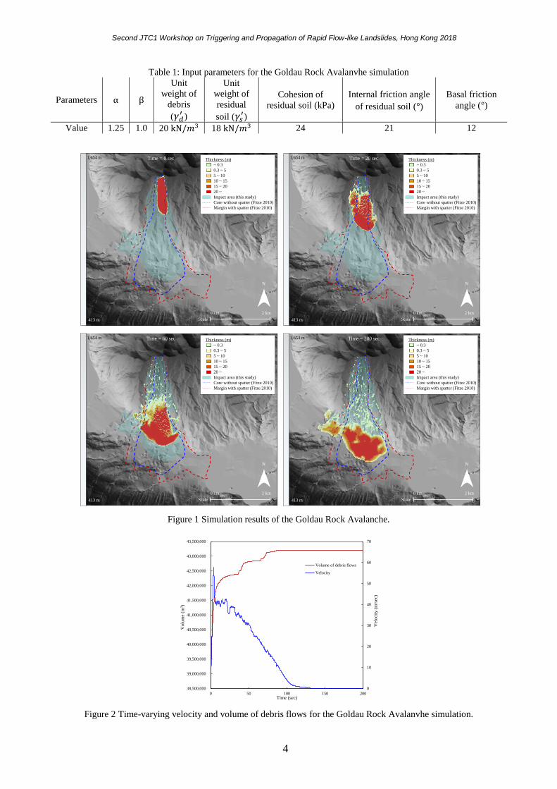
3.1 Goldau Rock Avalanche (A1)

The Goldau Rock Avalanche was simulated based on the provided topography and initial thickness of the

landslide. Initial soil depth of the study area was determined from 20 m to 100 m based on the detailed

longitudinal section of the study area of previous study conducted by Berner (2004). Cohesion and internal

friction angle of residual soil were determined based on previous study conducted by Thuro and Hatem (2010).

Basal friction angle was determined by Aaron and Hungr (2016). Parameters for the simulation were

summarized in Table 1. Figure 1 shows the topography and the debris profiles at different times of the Goldau

Rock Avalanche, and time-varying velocity and volume of debris flows are shown in Figure 2. The analytical

result of this study has a comparatively good agreement with those of the observation, but it is found that the

deposited debris are less scattered that the observed result. The velocity of the debris flow increased initially to

about 60 m/s and gradually decreased. The volume of debris increased from 38.5 Mm3 initially to 43 Mm3 by

entrainment of basin soil. The debris flow reached to downstream after about 100 seconds from the source area,

and at about 120 seconds, the velocity was nearly zero and deposited.


4

Table 1: Input parameters for the Goldau Rock Avalanvhe simulation

Parameters α β

Unit

weight of

debris

(𝛾𝑑′ )

Unit

weight of

residual

soil (𝛾𝑠′)

Cohesion of

residual soil (kPa)

Internal friction angle

of residual soil (°)

Basal friction

angle (°)

Value 1.25 1.0 20 kN/𝑚3 18 kN/𝑚3 24 21 12

Figure 1 Simulation results of the Goldau Rock Avalanche.

Figure 2 Time-varying velocity and volume of debris flows for the Goldau Rock Avalanvhe simulation.

413 m

1,654 m

N

2 km0 km

Scale

~ 0.3

0.3 ~ 5

5 ~ 10

10 ~ 15

15 ~ 20

20 ~

Impact area (this study)

Core without spatter (Fitze 2010)

Margin with spatter (Fitze 2010)

Thickness (m)Time = 0 sec

N

2 km0 km

Scale413 m

1,654 m

~ 0.3

0.3 ~ 5

5 ~ 10

10 ~ 15

15 ~ 20

20 ~





N

2 km0 km

Scale413 m

1,654 m

~ 0.3

0.3 ~ 5

5 ~ 10

10 ~ 15

15 ~ 20

20 ~





N

2 km0 km

Scale413 m

1,654 m

~ 0.3

0.3 ~ 5

5 ~ 10

10 ~ 15

15 ~ 20

20 ~





0

10

20

30

40

50

60

70

38,500,000

39,000,000

39,500,000

40,000,000

40,500,000

41,000,000

41,500,000

42,000,000

42,500,000

43,000,000

43,500,000

0 50 100 150 200

Vel

oci

ty (

m/s

ec)

Vo

lum

e (m

3)

Time (sec)

Volume of debris flows

Velocity


5

3.2 2008 Yu Tung Road debris flow, Hong Kong (C1)

The 2008 Yu Tung Road debris flow was simulated based on the provided topography and initial thickness

of the landslide. Initial soil depth of the study area was assumed from 3 m to 16 m based on the previous ground

investigation of detailed study report of the study area (Geo report No. 271). Cohesion and internal friction

angle of residual soil were determined based on the Geo report No. 271. Basal friction angle was determined

based on the previous study conducted by Raymond et al. (2017). Parameters for the simulation were

summarized in Table 2. Figure 3 shows the topography and the debris profiles at different times of the Yu Tung

Road debris flow. The time-varying volume of debris flow is also shown in Figure 4. Comparisons of time-

varying front location and the front velocity with previous studies and field observed values are shown in Figure

5 and 6. Figure 5 shows that the time-varying front location and the front velocity of debris flows by this study

have a good agreement with that of measured values and the previous study by Huang et al. (2017) and Kwan

et al. (2017). As shown in Figure 4, the volume of the debris flow increased from the initial 2,350 m3 to a

maximum of 3,480 m3, and gradually decreased as it deposited.

Table 2: Input parameters for the 2008 Yu Tung Road debris flow simulation

Parameters α β

Unit

weight of

debris

(𝛾𝑑′ )

Unit

weight of

residual

soil (𝛾𝑠′)

Cohesion of

residual soil (kPa)



Basal friction

angle (°)

Value 1.0 1.0 20 kN/𝑚3 18 kN/𝑚3 3 30 8

Figure 3 Simulation results of the 2008 Yu Tung Road debris flow.

Figure 4 Time varying debris volume.

0 m

100 m200 m300 m

400 m

500 m

~ 0.5

0.5 ~ 1

1 ~ 1.5

1.5 ~ 2

2 ~


0 m

253 m

N

0 m

100 m200 m300 m

400 m

500 m

~ 0.5

0.5 ~ 1

1 ~ 1.5

1.5 ~ 2

2 ~


0 m

253 m

N

0 m

100 m200 m300 m

400 m

500 m

~ 0.5

0.5 ~ 1

1 ~ 1.5

1.5 ~ 2

2 ~


0 m

253 m

N

0 m

100 m200 m300 m

400 m

500 m

~ 0.5

0.5 ~ 1

1 ~ 1.5

1.5 ~ 2

2 ~


0 m

253 m

N

0 m

100 m200 m300 m

400 m

500 m

~ 0.5

0.5 ~ 1

1 ~ 1.5

1.5 ~ 2

2 ~


0 m

253 m

N

0 m

100 m200 m300 m

400 m

500 m

~ 0.5

0.5 ~ 1

1 ~ 1.5

1.5 ~ 2

2 ~


0 m

253 m

N

0

500

1,000

1,500

2,000

2,500

3,000

3,500

4,000

0 10 20 30 40 50 60

Vo

lum

e (m

3)

Time (sec)

Volume of debris flows


6

Figure 5 Comparison of time-varying front location

of debris flows.

Figure 6 Comparison of debris front velocity.

3.3 Johnsons Landing debris avalanche, Canada (C2)

Johnsons Landing debris avalanche in Canada was simulated based on the provided topography and initial

thickness of the landslide. Cohesion, internal friction angle of residual soil and basal friction angle were assumed

to the values of the other landing debris avalanche case (C1). Basal friction angle for hypothesized high

resistance from trees zone defined by Aaron (2017) was assumed to 30°. Parameters for the simulation were

summarized in Table 3. Figure 7 shows the topography and the debris profiles at different times of Johnsons

Landing debris avalanche in Canada. The time-varying debris volume and average velocity are shown in Figure

8. As shown in Figure 7, debris flowing down from the upstream deposited on the bench, in the mid channel

and upper channel. From the result of this simulation indicated that 170,600 m3 of the debris deposited on the

bench, 53,961 m3 deposited in the mid channel and 4,795 m3 deposited in the upper channel, while it was

estimated that 169,000 m3 of debris deposited on the bench, 55,000 m3 deposited in the mid channel and 140,000

m3 deposited in the upper channel by Nicol et al. (2013). In this analysis, the amount of debris deposited on the

upper channel was considerably smaller than the observed result. The average velocity increased up to 35 m/s

in the upper channel and gradually decreased. When it reached the downstream, the velocity was about 15 m/s.

Nicol et al. (2013) also figured out that the rough flow velocities of the debris flow was between 25~35 m/s

based on the observation. The volume of the debris flow increased from the initial 320,000 m3 to a maximum

of 364,000 m3.

Table 3: Input parameters for the potential rock avalanche site in Canada

Parameters α β

Unit

weight of

debris

(𝛾𝑑′ )

Unit

weight of

residual

soil (𝛾𝑠′)

Cohesion of

residual soil (kPa)



Basal friction

angle (°)

Value 1.0 1.0 20 kN/𝑚3 18 kN/𝑚3 3 30 8,

30 (high resistance area)

0

100

200

300

400

500

600

0 5 10 15 20 25 30 35 40 45

Deb

ris

fro

nt

(m)

Time (s)

This study

Huang et al. (2017)

Measured

0

4

8

12

16

20

0 50 100 150 200 250 300 350 400 450 500 550

Fro

nt

vel

oci

ty (

m/s

)

Debris front (m)

This study

2d-DMM (Kwan 2017)

LS-DYNA (Kwan 2017)

Measured

448 m

1,541 m

~ 5

5 ~ 10

10 ~ 15

15 ~ 20

20 ~

Thickness (m)

Upper channel

Mid channel

Lower channel

Bench

N

1 km0 km

Scale

Time = 0 sec

448 m

1,541 m

~ 5

5 ~ 10

10 ~ 15

15 ~ 20

20 ~

Thickness (m)

Upper channel

Mid channel

Lower channel

Bench

N

1 km0 km

Scale

Time = 40 sec


7

Figure 7 Simulation results of Johnsons Landing debris avalanche, Canada.

Figure 8 Time-varying volume and average velocity of debris flows for Johnsons Landing debris avalanche in Canada.

3.4 A historical hillside catchment in Hong Kong (D1)

The historical hillside catchment in Hong Kong was simulated based on the provided topography and initial

thickness of the landslide. Two cases of no entrainment and entrained by debris were simulated. Total volume,

10,000 m3 deposited on the lower section applied to the source for the “with entrainment” case, and assumed

volume, 1,000 m3 applied to the source for the “without entrainment” case. Initial soil depth of the study area

was assumed from 2 m to 8 m based on the previous ground investigation of detailed study report (Geo report

No. 239). Cohesion, basal friction angle and internal friction angle of residual soil were also determined based

on the Geo report No. 239. Parameters for the simulation were summarized in Table 4. Figure 9 shows the

topography and the debris profiles at different times of the historical hillside catchment in Hong Kong. Time-

varying front location and the front velocity at point A, B and C are shown in Figure 10 and 11. The time-

varying volume of debris flow and average velocity of debris flows are also shown in Figure 12. The analytical

results show that the simulation results for the two cases are relatively similar, but the average velocity is smaller

for the “with entrainment” case that for the “without entrainment” case because the initial volume is small. It is

considered that this is due to the large inertia force from the beginning in the case of “without entrainment” case

in which the initial volume is largely applied. In the case of the “with entrainment” case, the initial volume

increased from 1,000 m3 to 10,290 m3 by entrainment. The thickness of the debris flow was maximum 6 m at

point A, 7~8 m at point B and maximum 4~5 m at point C, and the front velocity was distributed at 10~15 m/s.

Table 4: Input parameters for the historical hillside catchment in Hong Kong simulation

Parameters α β

Unit

weight of

debris

(𝛾𝑑′ )

Unit

weight of

residual

soil (𝛾𝑠′)

Cohesion of

residual soil (kPa)



Basal friction

angle (°)

Value 1.0 1.0 20 kN/𝑚3 18 kN/𝑚3 3 30 11

448 m

1,541 m

~ 5

5 ~ 10

10 ~ 15

15 ~ 20

20 ~

Thickness (m)

Upper channel

Mid channel

Lower channel

Bench

N

1 km0 km

Scale

Time = 80 sec

448 m

1,541 m

~ 5

5 ~ 10

10 ~ 15

15 ~ 20

20 ~

Thickness (m)

Upper channel

Mid channel

Lower channel

Bench

N

1 km0 km

Scale

Time = 100 sec

0

5

10

15

20

25

30

35

40

0

200,000

400,000

600,000

800,000

1,000,000

1,200,000

0 20 40 60 80 100 120V

eloci

ty (

m/s

ec)

Vo

lum

e (m

3)

Time (sec)

Volume of debris

Average velocity


8

Figure 11 Simulation results of the historical hillside catchment in Hong Kong.

Figure 9 Comparison of time-varying front location of debris flows.

Figure 10 Comparison of time-varying front velocity of debris flows.

Figure 12 Comparison of time-varying volume and average velocity of debris flows.

AB

C

146 m

485 m

~ 0.5

0.5 ~ 1

1 ~ 1.5

1.5 ~ 2

2 ~

Thickness (m)

0 sec

AB

C

146 m

485 m

~ 0.5

0.5 ~ 1

1 ~ 1.5

1.5 ~ 2

2 ~

Thickness (m)

0 sec

Without entrainment case With entrainment case

NN

AB

C

146 m

485 m

~ 0.5

0.5 ~ 1

1 ~ 1.5

1.5 ~ 2

2 ~

Thickness (m)

30 sec

AB

C

146 m

485 m

~ 0.5

0.5 ~ 1

1 ~ 1.5

1.5 ~ 2

2 ~

Thickness (m)

30 sec


NN

AB

C

146 m

485 m

~ 0.5

0.5 ~ 1

1 ~ 1.5

1.5 ~ 2

2 ~

Thickness (m)

60 sec

AB

C

146 m

485 m

~ 0.5

0.5 ~ 1

1 ~ 1.5

1.5 ~ 2

2 ~

Thickness (m)

60 sec


NN

0

1

2

3

4

5

6

7

8

0 10 20 30 40 50 60

Th

ick

nes

s (m

)

Time (sec)

Location A

Location B

Location C

Without entrainment case

0

1

2

3

4

5

6

7

8

0 10 20 30 40 50 60

Th

ick

nes

s (m

)

Time (sec)

Location A

Location B

Location C

With entrainment case

0

5

10

15

20

25

30

0 10 20 30 40 50 60

Vel

oci

ty (

m)/

s

Time (sec)

Location A

Location B

Location C


0

5

10

15

20

25

30

0 10 20 30 40 50 60

Vel

oci

ty (

m)/

s

Time (sec)

Location A

Location B

Location C


0

5

10

15

20

25

0

2,000

4,000

6,000

8,000

10,000

12,000

0 10 20 30 40 50 60

Vel

oci

ty (

m/s

ec)

Vo

lum

e (m

3)

Time (sec)

Volume

Average velocity


0

5

10

15

20

25

0

2,000

4,000

6,000

8,000

10,000

12,000

0 10 20 30 40 50 60

Vel

oci

ty (

m/s

ec)

Vo

lum

e (m

3)

Time (sec)

Volume

Average velocity



9

3.5 A potential rock avalanche site in Canada (D2)

The potential rock avalanche site in Canada was simulated based on the provided topography and initial

thickness of the landslide. Cohesion and internal friction angle of residual soil were assumed to the values of

the other rock avalanche case (Thuro and Hatem 2010). Basal friction angle was determined based on back-

analyzed values of rock avalanches by Aaron and Hungr (2016). Parameters for the simulation were summarized

in Table 4. Figure 13 shows the topography and the debris profiles at different times of the potential rock

avalanche site in Canada. The time-varying debris volume and average velocity are shown in Figure 14. As

shown in Figure 13, debris flowing down from the upstream showed a large impact on a flat area of downstream.

The average velocity increased up to 50 m/s in the upstream and gradually decreased. When it reached the

downstream, the velocity was about 10~20 m/s. The volume of the debris flow increased from the initial 8.3

Mm3 to a maximum of 12 Mm3, and after reaching the bottom, it did not increase more.

Table 5: Input parameters for the potential rock avalanche site in Canada

Parameters α β

Unit

weight of

debris

(𝛾𝑑′ )

Unit

weight of

residual

soil (𝛾𝑠′)

Cohesion of

residual soil (kPa)



Basal friction

angle (°)

Value 1.25 1.0 20 kN/𝑚3 18 kN/𝑚3 24 21 5.8

Figure 13 Simulation results of the potential rock avalanche site in Canada.

Figure 14 Time-varying volume and average velocity of debris flows of potential rock avalanche site in Canada.

200 m

1,911 m

~ 4

4 ~ 8

8 ~ 12

12 ~ 16

16 ~ 20

20 ~ 40

40 ~ 80

Thickness (m) N

1 km0 km

Scale

Time = 0 sec

200 m

1,911 m

~ 4

4 ~ 8

8 ~ 12

12 ~ 16

16 ~ 20

20 ~ 40

40 ~ 80

Thickness (m) N

0 km

Scale

Time = 40 sec

1 km

200 m

1,911 m

~ 4

4 ~ 8

8 ~ 12

12 ~ 16

16 ~ 20

20 ~ 40

40 ~ 80

Thickness (m) N

0 km

Scale

Time = 80 sec

1 km

200 m

1,911 m

~ 4

4 ~ 8

8 ~ 12

12 ~ 16

16 ~ 20

20 ~ 40

40 ~ 80

Thickness (m) N

0 km

Scale

Time = 100 sec

1 km

200 m

1,911 m

~ 4

4 ~ 8

8 ~ 12

12 ~ 16

16 ~ 20

20 ~ 40

40 ~ 80

Thickness (m) N

0 km

Scale

Time = 140 sec

1 km

200 m

1,911 m

~ 4

4 ~ 8

8 ~ 12

12 ~ 16

16 ~ 20

20 ~ 40

40 ~ 80

Thickness (m) N

0 km

Scale

Time = 180 sec

1 km

0

10

20

30

40

50

60

70

80

0

2,000,000

4,000,000

6,000,000

8,000,000

10,000,000

12,000,000

14,000,000

0 50 100 150 200

Vel

oci

ty (

m/s

ec)

Vo

lum

e (m

3)

Time (sec)

Volume of debris

Average velocity


10

4 CONCLUSIONS

In this study, a series of debris flows simulation was carried out by considering the soil erosion and fluid

dynamics. Navier-stokes momentum equation and continuity equation were used for the fluid mobility analysis,

and finite difference method was applied to solve the momentum and continuity equations. Rheological model

for non-Newtonian fluid was also applied, and the resistance of the debris flow was considered by a combination

of viscous and Coulomb friction. Soil erosion by debris flows was also calculated at each cell (point) and time.

As a result, the analytical results from this study, the development – erosion and entrainment – sedimentation

process of debris flow was analyzed for the benchmarking cases. In summary, it was found that the simulations

showed relatively reasonable results with the observations and the previous studies.

ACKNOWLEDGEMENTS

This work was supported by a Basic Science Research Program through the National Research Foundation of

Korea (NRF) funded by the Ministry of Education (No. 2018R1A6A1A08025348).

REFERENCES

Iverson, R. M. 1997. The physics of debris flows. Reviews of geophysics, 35(3): 245-296.

Jakob, M., & Friele, P. 2010. Frequency and magnitude of debris flows on Cheekye River, British Columbia.

Geomorphology, 114(3): 382-395.

Hilker, N., Badoux, A., & Hegg, C. 2009. The Swiss flood and landslide damage database 1972-2007. Natural

Hazards and Earth System Sciences, 9(3): 913.

Aaron, J. 2017. Advancement and Calibration of a 3D Numerical Model for Landslide Runout Analysis, PhD

Thesis. University of British Columbia.

Berner, C. 2004. Der Bergsturz von Goldau, Diploma Thesis. ETH, Zurich.

Fitze, P. 2010. Runout analysis of rapid, flow-like landslides, Master’s Thesis. Hochschule für Technik

Rapperswil.

Thuro, K. K., Berner, C., & Eberhardt, E. 2006. Der Bergsturz von Goldau 1806 - Was wissen wir 200 Jahre

nach der Katastrophe? Bull. Angew. Geol., 11(2): 13–24.

The Government of the Hong Kong Special Administrative Region. 2012. Detailed study of the 7 June 2008

landslides on the hillside above Yu Tung Road, Tung Chung (Georeport No. 271). Hong Kong.

Law, R. P., Kwan, J. S., Ko, F. W., & Sun, H. W. 2017. Three-dimensional debris mobility modelling coupling

smoothed particle hydrodynamics and ArcGIS.

Dai, Z., Huang, Y., Cheng, H., & Xu, Q. 2017. SPH model for fluid–structure interaction and its application to

debris flow impact estimation. Landslides, 14(3): 917-928.

Song, D., Ng, C. W. W., Choi, C. E., Zhou, G. G., Kwan, J. S., & Koo, R. C. H. 2017. Influence of debris flow

solid fraction on rigid barrier impact. Canadian geotechnical journal, 54(10): 1421-1434.

Nicol, D., Jordan, P., Boyer, D., & Yonin, D. 2013. Regional District of Central Kootenay ( RDCK ) Johnsons

Landing Landslide Hazard and Risk Assessment.

The Government of the Hong Kong Special Administrative Region. 2008. Detailed study of the 22 August 2008

landslide and distress on the natural hillside at Kwun Yam Shan, below Tate’s ridge (Georeport No. 239).

Hong Kong.

Benchmarking exercise of landslide runout analysis considering …JTC1... · 2018-11-08 · The...

Documents

Transcript of Benchmarking exercise of landslide runout analysis considering …JTC1... · 2018-11-08 · The...