Asian Development Bank Institute · α = capital share, GDP = gross domestic product, K/L = capital...

ADBI Working Paper Series

TRANSITIONING FROM LOW-INCOME GROWTH TO HIGH-INCOME GROWTH: IS THERE A MIDDLE-INCOME TRAP?

David Bulman, Maya Eden and Ha Nguyen

No. 646 January 2017

Asian Development Bank Institute

The Working Paper series is a continuation of the formerly named Discussion Paper series; the numbering of the papers continued without interruption or change. ADBI’s working papers reflect initial ideas on a topic and are posted online for discussion. ADBI encourages readers to post their comments on the main page for each working paper (given in the citation below). Some working papers may develop into other forms of publication.

Suggested citation:

Bulman, D., M. Eden and H. Nguyen. 2016. Transitioning from Low-Income Growth to High-Income Growth: Is There a Middle-Income Trap?. ADBI Working Paper 646. Tokyo: Asian Development Bank Institute. Available: https://www.adb.org/publications/transitioning-low-income-growth-high-income-growth Please contact the authors for information about this paper.

Email: [email protected], [email protected], [email protected]

David Bulman, Maya Eden, and Ha Nguyen are economists from the Development Research Group at the World Bank.

The views expressed in this paper are the views of the author and do not necessarily reflect the views or policies of ADBI, ADB, its Board of Directors, or the governments they represent. ADBI does not guarantee the accuracy of the data included in this paper and accepts no responsibility for any consequences of their use. Terminology used may not necessarily be consistent with ADB official terms.

Working papers are subject to formal revision and correction before they are finalized and considered published.

Asian Development Bank Institute Kasumigaseki Building, 8th Floor 3-2-5 Kasumigaseki, Chiyoda-ku Tokyo 100-6008, Japan Tel: +81-3-3593-5500 Fax: +81-3-3593-5571 URL: www.adbi.org E-mail: [email protected] © 2016 Asian Development Bank Institute

mailto:[email protected]

ADBI Working Paper 646 Bulman, Eden and Nguyen

Abstract Is there a “middle-income trap”? Theory suggests that the determinants of growth at low and high income levels may be different. If countries struggle to transition from growth strategies that are effective at low income levels to growth strategies that are effective at high income levels, they may stagnate at some middle income level; this phenomenon can be thought of as a “middle-income trap.” Defining income levels based on per capita gross domestic product relative to the United States, we do not find evidence for (unusual) stagnation at any particular middle income level. However, we do find evidence that the determinants of growth at low and high income levels differ. These findings suggest a mixed conclusion: middle-income countries may need to change growth strategies in order to transition smoothly to high income growth strategies, but this can be done smoothly and does not imply the existence of a middle-income trap. JEL Classification: O47, O40


Contents

1. INTRODUCTION ....................................................................................................... 1

2. DEBATING THE MIDDLE-INCOME TRAP: THEORY AND EMPIRICS ..................... 3

3. IDENTIFYING A MIDDLE-INCOME TRAP: BASIC FACTS ON INCOME DYNAMICS .......................................................................................... 6

4. COMPARING MIDDLE INCOME AVERAGE GROWTH BASED ON FUNDAMENTALS ............................................................................................. 11

5. REGRESSION ANALYSIS ...................................................................................... 17

6. CONCLUSION ......................................................................................................... 18

REFERENCES ................................................................................................................... 20

APPENDIX .......................................................................................................................... 22


1

1. INTRODUCTION Policy and academic communities in recent years have expressed growing concern that countries at middle income levels may fail to generate enough growth to become high-income countries. In these countries, the policies that facilitated growth from low income to middle income might not facilitate a transition from middle income to high income, resulting in a “middle-income trap.” Yet while theory suggests that growth determinants may differ by income level, empirical evidence for middle-income traps has not been conclusive.

Middle-income countries seek policies that can help them achieve strong and sustained growth and eventually help them join the league of high-income countries. Yet finding a set of appropriate pro-growth policies is a complicated task, particularly given the uniqueness of every country’s institutional constraints. This paper does not lay out specific policy recommendations; rather, it provides a set of stylized facts about middle-income countries and about fundamentals that might facilitate the transition from middle to high income. We focus on changes in relative income (i.e., how countries catch up to other high-income countries), rather than absolute income.

We find mixed evidence regarding the existence of a middle-income trap—i.e., slowing growth that might cause middle-income countries to stagnate prior to joining the high income group. The predominant evidence against the existence of such a middle-income trap comes from an examination of the growth paths of successful transitions. We find that “escapees”—countries that “escaped” the middle-income trap and became rich—tend to grow fast and consistently to high income, and do not stagnate at any point as a middle-income trap theory would suggest. In contrast, “non-escapees” tend to have low growth at all levels of income. In other words, while the existence of a middle-income trap implies that growth rates systematically slow down as countries reach middle income status, no such systematic slowdown is apparent in the data.

However, our analysis does show that successful middle-income countries (i.e., those that “escape” and become high income) have different growth fundamentals and different policy choices than unsuccessful middle-income countries (i.e., those that are still middle income or that have become low income). Among middle-income countries, descriptive analyses suggest the following factors associated with higher growth: (i) economic structure, and in particular a faster transformation from agriculture to industry; (ii) higher export shares; (iii) lower inflation; and (iv) decreases in inequality and dependency ratios. We also find evidence that the effectiveness of different growth strategies may vary across income levels. This is consistent with middle-income trap theories suggesting that middle-income countries get stuck in the transition from growth strategies that are effective at low income levels to growth strategies that are effective at high income levels. While we do not find evidence of being “stuck,” we do find evidence that such a transition may be needed.

We find that total factor productivity (TFP) growth is a much larger source of economic growth, both in absolute and relative terms, in middle- and high-income countries than in low-income countries.1 This highlights the limits of capital accumulation (after all, investment has a decreasing marginal return) and suggests the important roles of

1 This is true regardless if human capital is included or excluded from the production function (see Data

Appendix for more details).


2

education, research and innovation, and structural reforms. Figure 1 presents average contributions to annual growth in output per worker, by income level.2 The orange part represents average annual TFP growth and the blue part represents average annual growth of the capital–labor ratio (multiplied by the capital share). For low-income countries, the overwhelming majority of growth comes from capital accumulation. For middle- and high-income countries, however, the share of TFP growth is much larger.

Figure 1: Average Contributions to Growth, by Income Level

α = capital share, GDP = gross domestic product, K/L = capital per worker, TFP = total factor productivity. Source: Authors’ calculations based on Penn World Table Version 7.0 (see Data Appendix).

The observation makes sense. For low-income countries, since the level of capital is still low, it is relatively easier to attract and accumulate more capital (think of giving farmers tractors). When the level of capital accumulation is higher, it is harder to attract investment because the return to capital now becomes lower (i.e., it doesn’t help to give one farmer two tractors). To maintain growth, countries have to turn to other sources: better technologies, better management practices, and research and innovation. Our conjecture is that countries with better strategies to access or, even better, generate state-of-the-art technologies and management practices will be able to catch up to high-income countries. While this aggregate finding is consistent with the above economic intuition, we fail to find strong support for it on a more disaggregated level. We conduct a regression analysis of growth determinants in low and middle income levels. Our findings do not support the hypothesis that innovation and human capital accumulation are more important determinants of growth for middle-income countries compared with low-income countries. Rather, the regressions suggest that growth of low- and middle-income countries may have to do more with the transformation of the economy: the growth effect of moving from agriculture to industry is stronger for middle-income

2 Here, as in the rest of the paper, we define low-income countries as those with per capita incomes less

than 10% of the United States (US); middle-income countries as those with per capita incomes between 10% and 50% of the US; and high-income countries as those with per capita incomes over 50% of the US. Here, we further divide middle-income countries into lower- and upper-middle-income countries using a threshold of 30% of the US. Table A.1 in the Appendix lists economies by income group at 2009. The categorization looks reasonable.


3

countries than for low-income countries, while the growth effect of moving to services is weaker for middle-income countries.

The empirical analysis is not only of academic interest; a middle-income “trap” implies income stagnation for much of the 70% of the world’s population currently living in middle-income countries. Such growth stagnation would have major human and global consequences. Understanding the correlates of successful middle income growth helps points to directions for future work that develops policy frameworks. For example, the concept of middle-income traps is used to formulate policy recommendations for continued economic growth in the People’s Republic of China (PRC) (World Bank 2013) and in Malaysia (Flaaen, Ghani, and Mishra 2013).

The paper is organized as follows: section 2 reviews related literature on the middle-income trap. Section 3 presents basic descriptions of income dynamics for a large set of countries, with a particular focus on the middle income group. Section 4 contrasts middle-income “escapees” and “non-escapees” along several dimensions and compares middle-income country growth based on fundamentals. Section 5 presents regression results comparing growth determinants at middle income and low income levels. Section 6 concludes.

2. DEBATING THE MIDDLE-INCOME TRAP: THEORY AND EMPIRICS

The term “middle-income trap” first appeared in the World Bank’s An East Asian Renaissance: Ideas for Economic Growth, which stated that “middle income countries…have grown less rapidly than either rich or poor countries” (Gill and Kharas 2007). Since then, the concept of a middle-income trap has become increasingly popularized and discussed in both popular media3 and academic literature, although a consensus on the validity of the concept has yet to emerge.

The middle-income trap concept has been debated from both theoretical and empirical angles. Theoretically, middle-income countries may face particular challenges in transitioning their economic growth models from strategies that were successful while they were poor to strategies that enable them to directly compete with high-income countries. In this sense, middle-income traps reflect the difficulty middle-income countries have competing with either low-wage economies or highly skilled advanced economies. These countries need different growth strategies, and these strategies are not readily available. At low income levels, countries require structural transformation, reallocation, and the availability of jobs. At middle income levels, the gains from reallocating surplus labor begin to evaporate, in the vein of a Lewis–Kuznets framework—without surplus labor, wages begin to rise, making low-cost exports less competitive. Additionally, returns to capital begin to fall as the gains from technological imitation and importing foreign technology decline (Agenor and Canuto 2012, Kharas and Kohli 2011).

New sources of productivity, and particularly local innovation, are required to maintain growth and diversity exports. The previous section highlighted the greater contribution of TFP growth to overall growth for middle- and high-income countries. TFP growth slowdowns in middle-income countries are identified as a key cause for overall growth slowdown: Eichengreen et al. (2012) find that, on average, 85% of a fast-growing 3 See, for example, The Economist (23 June 2011) for the People’s Republic of China’s “Middle

Income Trap,” and other media coverage for other countries (the Russian Federation, Malaysia, and Latin America).


4

economy’s slowdown is attributable to TFP, and only 15% to capital accumulation. Daude and Fernandez-Arias (2010) show that slow productivity growth, rather than factor accumulation, explains the inability of middle-income countries in Latin America to close the income gap with advanced economies. Felipe, Abdon, and Kuman (2012) find that countries that make it to the upper-middle-income group tend to have a more “diversified, sophisticated, and non-standard export basket” than those that remain stuck at lower-middle income levels.4

Combining the innovation and export approaches into a framework for middle income growth, Kharas and Kohli (2011) argue in terms of the supply and demand needs of an economy, with low-income countries focused more on supply and high-income countries focused on demand. Low-income economies seek to maximize factor inputs through extensive growth while also focusing on the supply of an enabling institutional environment. Middle-income countries instead focus on demand: domestic demand through growth of the middle class, and new export demand focused on innovation and product differentiation. Creation of these new sources of demand requires “modern and more agile institutions for property rights, capital markets, successful venture capital, competition, and a critical mass of highly skilled people to grow through innovations.”

Although there is considerable theoretical evidence that middle-income countries need to transition growth strategies to maintain growth and become high income, empirical evidence that middle-income countries are more likely to stagnate than countries at other income levels has been less conclusive. There have been two general empirical approaches to identifying the existence of middle-income traps. The first strand does not explicitly refer to “traps,” but rather analyzes cross-country growth dynamics across income levels, attempting to identify criteria for growth slowdowns and accelerations. The second strand directly confronts the definitional question implied by the middle-income trap hypothesis: are middle-income countries particularly cursed in failing to grow to high income? The first approach focuses predominantly on absolute incomes, comparing growth trajectories within a country. The second approach focuses predominantly on relative incomes, comparing growth to a high income benchmark.

Considerable research has tried to document growth patterns for low- and middle-income countries. Pritchett (2000) shows that the patterns for developing countries are best characterized as volatile. While some countries have steady growth (hills and steep hills), others have rapid growth followed by stagnation (plateaus), rapid growth followed by decline (mountains) or even catastrophic falls (cliffs), continuous stagnation (plains), or steady decline (valleys). This suggests that econometric growth literature that makes use of the panel nature of data is unlikely to be informative—a point previously made by Easterly et al. (1993). In that paper, it is shown that growth is volatile across decades while country characteristics are much more stable, and growth is largely driven by external shocks. Pritchett and Summers (2014) follow and corroborate Easterly et al. (1993), finding a tendency for regression to the mean for fast-growing countries. The paper also finds that income levels are poor predictors of growth slowdowns; the key is the fundamental difficulty of progress at all stages.

Following Pritchett’s (2000) suggestions, Hausmann et al. (2005) look for instances of rapid, but sustained, acceleration in economic growth. They find that growth accelerations tend to be correlated with increases in investment and trade, and with real exchange rate depreciations. Growth accelerations are also correlated with political regime changes and economic reforms. At the same time, growth

4 Vivarelli (2014) provides a comprehensive discussion on the challenges faced by middle-income

countries, with particular attention paid to the role of developing innovation capacity.


5

accelerations are highly unpredictable; a majority of reforms do not lead to growth acceleration.

Related to growth accelerations, recent literature focused largely on middle-income countries specifically analyzes growth slowdowns. Eichengreen et al. (2012) construct a sample of cases where fast-growing economies slow down. They show that rapidly growing economies slow down significantly when their per capita incomes reach around $16,000 in year-2005 constant international prices. Since the PRC will soon reach this level of income, the paper implies that the PRC will likely witness a slowdown. In a recent paper, Cai (2012), through a discussion of many of the PRC’s current problems, shares this concern. And in a more recent paper, Eichengreen et al. (2013) instead identify two nodes for growth slowdowns, one at $10,000–$11,000 and one at $15,000–$16,000, concluding that middle-income countries experience slowdowns in stages rather than at a single point in time. Aiyar et al. (2013) look explicitly at different growth patterns in middle-income countries, finding that growth slowdowns are more likely for middle-income countries than for low- or high-income countries. Using 42 explanatory variables to explain slowdowns, they find that small government size, deregulation, and infrastructure development are particularly important for middle-income slowdowns as opposed to low- and high-income slowdowns.

This literature on growth accelerations and slowdowns uses panel data to focus on growth patterns within individual countries; however, identifying an income-level “trap” instead requires comparing growth against a high income benchmark, as income-level thresholds are frequently redefined. For instance, Eichengreen et al. (2012, 2013) and Aiyar et al. (2013) focus on growth relative to previous growth; however, the authors do not control for levels of past period growth, so in their specification, slowdowns do not necessarily imply income-level traps, especially considering that middle-income countries in their data have higher first-period growth. For instance, a country that slows from 10% annual growth to 5% annual growth will still develop rapidly enough to catch up to high-income economies. Indeed, several countries forming the basis for the analysis of Eichengreen et al. (2012, 2013) are now high-income countries, including the Republic of Korea and Taipei,China. The PRC, often the implicit (or explicit) focus of growth slowdown papers, has already slowed to a “new normal” growth path that is more than 3 percentage points slower than growth over the last decade, but this new “slow” growth of 7% would allow the PRC to reach high income status in 8 years (absolute) or 16 years (relative to United States [US] income).5

Other literature on middle-income traps focuses specifically on the movement of countries to high income status, defined by either absolute or relative income levels, i.e., thresholds based on constant dollar values and thresholds based on income relative to high-income countries. Felipe, Abdon, and Kuman (2012) group countries into four income categories—low, lower-middle, upper-middle, and high—and then define lower- and upper-middle-income traps by the amount of time it takes a country to reach the next income levels: lower-middle-income countries that remain lower-middle income for 28 years are “trapped,” as are upper-middle-income countries that have not become high income in 14 years. However, these thresholds are based on the median number of years that all countries spent at particular income levels—similar thresholds can be constructed at any income level, so it is not clear that there is any particular growth dynamic characterizing countries and middle income

5 Here, the threshold for high income is based on the 2014 World Bank value of $12,746 gross national

income (GNI) per capita using the Atlas method. The relative income threshold is based on 50% of US GNI per capita (at purchasing power parity), and assumes 2% annual US growth.


6

levels. Note that in looking at absolute income, every country with even slightly positive growth will eventually become high income—so the criteria for a “trap” has to be the speed of this transition.

More recently, Im and Rosenblatt (2013) discuss the definition of middle-income traps and explore both the absolute and relative thresholds of the “traps.” Using a transitional matrix analysis, they also find little support for the idea of middle-income traps, and they demonstrate that transitions from lower-middle income to upper-middle income are as likely as transitions from upper-middle income to high income.

In sum, the existing literature identifies several theoretical reasons why middle-income countries may face particular challenges in maintaining high growth rates and transitioning to high income, but empirical evidence on a “trap” is mixed. We do not believe the theoretical and empirical findings are at odds. In the following sections, we demonstrate that, although empirically there is no evidence that middle-income countries are more likely to stagnate than countries at other income levels, nevertheless middle-income countries that grow fast and achieve high income have different growth fundamentals than low-income countries or than countries that stagnate at middle income: in other words, the theoretical concerns are valid, but countries can and have responded and avoid stagnation.

3. IDENTIFYING A MIDDLE-INCOME TRAP: BASIC FACTS ON INCOME DYNAMICS

In this section, we present some stylized facts on countries’ income dynamics to identify whether such income dynamics correspond to an identifiable growth slowdown, or trap, at middle income levels. The literature above highlights three potential approaches to identify an income trap: (i) slowdown relative to past growth, (ii) the persistence of an absolute income level, and (iii) the persistence of a relative income level. All three approaches have advantages, though they analyze different questions. For both theoretical and practical reasons, we believe that the use of relative income makes the most sense for determining whether a middle-income trap exists. Theoretically, as highlighted above, the key reason for a middle-income trap is failure to transition from low-wage growth strategies to high-wage growth strategies; these wages are determined internationally on a relative scale. Practically, the use of an absolute threshold implies that any positive growth will eventually yield a transition to high income, even if such growth is well below the global and high income average. For these reasons, we focus on relative incomes.

To identify income dynamics, we first divide countries into three relative income groups: low, middle, and high. Using a relative scale, low-, middle-, and high-income countries are those that have purchasing power parity (PPP) gross domestic product (GDP) per capita less than or equal to 10%, between 10% and 50%, and above 50% of US PPP GDP per capita, respectively. Table A.1 in the Appendix lists all economies in these three categories in 2009 (including narrow relative income bins as well).

We remove oil exporters from our analysis for two reasons. First and more importantly, growth of these countries is driven largely by oil exports and not so much by fundamentals. Second, proceeds from oil exports can be very volatile, which would distort the persistence of countries’ relative income. The Data Appendix provides a list of oil exporters removed from the sample.


7

Figure 2: Relative Income Dynamics, 1960–2009

GRC = Greece; HKG = Hong Kong, China; IRE = Ireland; JPN = Japan; KOR = Republic of Korea; PRI = Puerto Rico; SIN = Singapore; SPA = Spain; SYC = Seychelles; TAP = Taipei,China. Note: “Escapee” countries in orange. Source: Authors’ calculations based on Penn World Table Version 7.0 (see Data Appendix).

Figure 2 shows economies’ long-run changes of their income relative to the US. The log of per capita income relative to the US in 1960 is on the x axis, with the 2009 value on the y axis. Each axis is divided into three areas, representing the three income groups. Economies in the top-middle quadrant (in orange) are those that “escaped” from middle income to high income over this period. The list of escapees includes Greece; Hong Kong, China; Ireland; Japan; the Republic of Korea; Puerto Rico; Seychelles; Singapore; Spain; and Taipei,China. Two countries that nearly make the list (the top of the middle quadrant) are Portugal and Cyprus, which are still classified as middle income in 2009. Table 1 summarizes the number of countries by income level and subsequent income transition in 1960 (and alternatively, in 1970, where we have more data).

The predominant fact that emerges from Figure 2 and Table 1 is that relative income levels are highly persistent. All high-income countries in 1960 remained high income in 2009; a majority of middle-income countries remained middle income;6 and only a handful of low-income countries joined the middle income group. A concern is that there might have been more fluid movements of countries between 1960 and 2009—for example, some countries might have moved to high income and moved back, which Figure 1 would fail to capture. Figure A.1 in the Appendix shows that there are few such movements. Almost all of the countries that have ever moved into high income have stayed there. Two exceptions are the Czech Republic and Lebanon.7 Another potential concern is that this persistence is an artifact of our selected middle income threshold (i.e., 10%–50% of US per capita GDP). Figure A.2 in the Appendix shows that this is not the case: relative income mobility is no more persistent for middle-income countries than other countries regardless of the threshold selected. In

6 A few middle-income countries declined to poor income groups (Bolivia, Ghana, Haiti, Honduras,

Nicaragua, Paraguay, and Zambia). 7 Czech Republic was a high-income country (52% of the US) in 1990, but then it dropped to middle

income throughout the 1990s and early 2000s, and, since 2005, it has again been high income. Lebanon became rich in the mid-1970s but went to middle income in the early 1980s as it had a long civil war in the 1980s.


8

fact, through low and middle income, income levels become decreasingly persistent as countries get wealthier (i.e., low income levels are the most persistent, lower-middle income levels are slightly less persistent, and upper-middle income levels are even less persistent).

Table 1: Countries’ Income Distribution, 1960 and 1970

Base Year

1960 1970 # of countries in sample Low income 42 59 Middle income 41 58 High income 19 26 Total 102 143 # (%) of income group transitions, base year to 2009 Low Low 37 (88.1%) 50 (84.7%) Low Middle 5 (11.9%) 9 (15.3%) Low High 0 (0.0%) 0 (0.0%) Middle Low 7 (17.1%) 8 (13.8%) Middle Middle 24 (58.5%) 41 (70.7%) Middle High 10 (24.4%) 9 (15.5%) High Low 0 (0.0%) 0 (0.0%) High Middle 0 (0.0%) 1 (3.8%) High High 19 (100.0%) 25 (96.2%)

Source: Authors’ calculations based on Penn World Table Version 7.0 (see Data Appendix).

We also observe that escapees grow faster than non-escapees at all levels of income. Figure 3 shows the average annual growth rates at different per capita income levels relative to the US (shown in the x-axis). The orange columns are the average growth rates for countries that ever escape from middle to rich, and the blue columns represent growth rates for those countries that never escape. The escapees do consistently much better than their non-escapee counterparts, and they do not exhibit significant signs of slowing down. In contrast, non-escapees have low and stable growth over all levels of income: they too do not show signs of slowing down at middle income.

Figure 3 presents evidence against the existence of a middle-income trap that causes growth to stagnate at a particular income level. Rather, non-escapees on average have slower growth at all levels of income, suggesting a persistent role of country-specific constraints and policy problems. A very familiar graph reinforces the point. Figure 4 shows the levels of PPP GDP per capita for escapees and some notable non-escapees over time. One can see that escapees, as a whole, grow strongly toward high income and do not see a “middle-income trap,” while selected key non-escapees (Mexico, Malaysia, Brazil, Turkey) experience relative stagnation for the entire period.


9

Figure 3: Average Annual Change of Purchasing Power Parity Gross Domestic Product per Capita

GDP = gross domestic product. Sources: Penn World Table Version 7.0; Authors’ calculations (see Data Appendix).

Figure 4: Income Dynamics of Escapees vs. Non-Escapees

GDP = gross domestic product. Note: The list of economies on the right-hand side is sorted by 2009 income level. Source: Authors’ calculations based on Penn World Table Version 7.0 (see Data Appendix).

Another graph reinforces the notion that economies do not slow down at middle income levels (relative to the US). Figure 5 shows a scatter plot of countries’ subsequent 10-year average growth against (log of) countries’ initial income relative to the US in 1960, 1970, 1980, 1990, and 2000. Evidence for a middle-income trap would imply a U-shaped curve, with countries systematically slowing down at middle income levels. We do not see such evidence.


10

Figure 5: Initial Relative Income and Growth


For escapees, GDP growth was high and sustainable—strong growth in one period was followed by strong growth in the subsequent period—as if previous high growth paves the way for subsequent growth. This “momentum” hypothesis stands in contrast to the “regression to the mean” finding of Pritchett and Summers (2013). A look at all countries confirms empirically the momentum hypothesis: there is a correlation between previous growth and current growth. Figure 6 shows the scatter plot of a middle-income country’s average decadal growth rates in two consecutive decades. The x axis presents average growth over t-10 through t-1, while the y axis presents average growth from t+1 through t+10, for all available years. The orange dots correspond to those countries that escaped from the middle income to the high income group. For all middle-income countries, there is a significant, positive correlation between lagged and current decadal growth rates. The correlation coefficient for middle-income escapees is 0.47, while the correlation coefficient for middle-income non-escapees is 0.25. 8 The positive correlation we find is particularly strong for escapees. Also for escapees, the dots are much more concentrated at the upper right end of the scatter plot, implying that the escapees’ GDP growth is not only higher, but also more stable than that of other countries.

There are several possible economic interpretations for the persistence in growth. For example, it is possible that high growth provides more resources for investment (in infrastructure and education), paving the way for high growth in the next period. Political economy may also play a role: it may be politically easier for reforms to continue and deepen if they yielded economic success and high growth in the previous period.

8 For all low- and middle-income countries, using non-overlapping decadal growth, the correlation

coefficient between lagged and future growth is 0.19. Easterly et al. (1993) calculate the correlation coefficient between 1960s–1970s for developing countries as 0.1 and 1970s-–1980s as 0.33.


11

Figure 6: Growth Correlation for Middle-Income Countries (%)


4. COMPARING MIDDLE INCOME AVERAGE GROWTH BASED ON FUNDAMENTALS

What determines the ability of certain middle-income countries to persist in high growth? The previous section demonstrated that using a relative income standard, there is not an easily identifiable middle-income trap; instead, there are successful and unsuccessful countries at all levels of income.

Here, we first document several differences in fundamentals of escapees (middle-income countries that successfully transitioned to high-income countries) and non-escapees (middle-income countries that have yet to transition). 9 Such an exercise enables an identification of the underlying characteristics and sources of growth associated with movements from middle income to high income. Results from this analysis are shown in the Appendix, Table A.2. In the table, significant differences (at 95%) between escapees and non-escapees are represented in bold text. In addition to the results for all middle-income countries, Table A.2 also presents disaggregates escapee and non-escapee fundamentals across four middle-income categories (10%–20%, 20%–30%, 30%–40%, and 40%–50% of US income).

This descriptive analysis reveals that escapees have higher GDP and TFP growth at all relative income levels. They have greater levels of human capital, experience a faster transformation to industry, are consistently export-oriented, have better macroeconomic management, and have more income equality and more growth-conducive demographic conditions. Additional details are discussed in the following subsections.

9 Unlike the previous list of escapees, which only included economies that “escaped” between 1960

and 2009, this list includes economies that escaped earlier as well as economies for which we do not have 1960 data. These include Austria; Bahamas; Spain; Finland; Greece; Hong Kong, China; Ireland; Iceland; Israel; Italy; Japan; the Republic of Korea; Macau, China; Malta; Puerto Rico; Singapore; Slovenia; Seychelles; and Taipei,China.


12

However, the approach represented in Table A.2 suffers from a potential methodological shortcoming. If we think of escapees as rapidly growing countries, then the table basically shows that fast-growing countries have better fundamentals than slow-growing countries. These associations could be very misleading about the causal impact of the fundamentals. For instance, advocates like to point out that fast-growing countries like the Republic of Korea engaged in industrial policy, but this ignores the fact that many countries have experimented with industrial policy without growing rapidly.

The remainder of this section therefore looks at growth performance based on fundamentals, rather than the reverse. In the following discussion, each chart represents one potential determinant of future growth. Here, the blue bars represent average growth trajectories (future 10-year average growth rates) for countries with values below the median for that particular characteristic, and the orange bars represent average growth trajectories for countries with values above the median. The error bars represent 95% confidence intervals. We separate results for lower-middle-income countries (10%–30% of US income) and upper-middle-income countries (30%–50% of US income) to see how growth determinants differ across the middle income spectrum. Medians are calculated on an annual basis for lower- and upper-middle-income countries separately. So, for instance, in Figure 7A, the blue bars represent the average future 10-year average growth rates for all country/year observations in which the level of tertiary education is lower than the median value for all lower- and upper-middle-income countries in that particular year.

Human Capital The results in Table A.2 indicate that escapees exhibit higher levels of primary, secondary, and tertiary education, and are also clearly differentiated from non-escapees by the number of patents they generate. Disaggregated results suggest that tertiary education is more important for escapees at lower-middle income levels, while patents are more prevalent for escapees at upper-middle income levels. This finding suggests that the quality of education is more important at middle-high income levels, consistent with the view that transition from middle to high income must be fueled by innovation-led growth.

Looking instead at growth performance based on fundamentals, shown in Figures 7A and 7B, average years of tertiary education has little predictive power with regard to future growth; in the slight (not statistically significant) differences, upper-middle-income countries seem to suffer slightly from more tertiary education. With regard to patents, both lower-middle-income countries and upper-middle-income countries with above-median patents grow slower. This contrasts with the escapee vs. non-escapee results, which showed that upper-middle-income-level escapees have many more patents than non-escapees. The results in Table A.2 were driven by the patent performance of the Republic of Korea and Japan, which is why this current exercise adds value.


13

Figure 7A: Average Years of Tertiary Schooling Relative to the United States

(beginning of period) Figure 7B: Number of Patents

(beginning of period)

Notes: Error bars represent 95% confidence intervals. “Below” (“above”) refers to observations below (above) the median in a given year for the given income group. LMI refers to lower-middle-income countries; UMI refers to upper-middle-income-countries. “Beginning of period” indicates observations at the start of a given 10-year growth period. Source: Authors’ calculations (see Data Appendix).

Economic Structure Countries that escape seem to show a clear and rapid transition from agriculture to industry, and this transition is particularly prevalent at lower-middle income levels (Table A.2). Escapees tend to have larger industry sectors and smaller agriculture and service sectors, and they also have higher growth in industry and lower growth in agriculture and services. Buttressing these findings, Figures 8A and 8B show that lower-middle-income countries that see larger declines in the agriculture share and increases in the industry share grow much faster on average, while an increase in the share of the service sector translates into slower growth; these trends hold for the upper-middle income level, but are reduced in magnitude.

Figure 8A: Growth in Agriculture Share of Gross Domestic Product

(concurrent 10-year annual average)

Figure 8B: Growth in Industry Share of Gross Domestic Product


Notes: Error bars represent 95% confidence intervals. “Below” (“above”) refers to observations below (above) the median in a given year for the given income group. LMI refers to lower-middle-income countries; UMI refers to upper-middle-income-countries. Source: Authors’ calculations (see Data Appendix).


14

Openness Escapees are significantly more export-oriented and have more undervalued currencies (defined as in Rodrik 2008). This undervaluation is particularly prevalent at lower-middle income (Table A.2). For both lower- and upper-middle-income countries, export orientation is associated with higher growth and undervaluation is associated with lower growth (Figures 9A and 9B). These trends are particularly strong for upper-middle-income countries.

Figure 9A: Exports as a Share of Gross Domestic Product

(concurrent 10-year annual average) Figure 9B: Log Undervaluation



Macroeconomic Conditions Escapees, and particularly upper-middle-income escapees, do not experience high inflation (Table A.2). No middle-income “eventual escapee” ever experiences inflation over 20%, and by the time they reach upper-middle income levels, they very rarely experience inflation over 10%. Even excluding the outliers (defined as the top 5% of observations), middle-income escapees experience lower inflation than non-escapees.10 However, escapees have higher levels of external debt, which might be a result of greater access to outside markets or more financial development. Due to a lack of data, we cannot include other financial development indices.

Looking instead at growth based on fundamentals, countries with lower levels of inflation grow significantly faster (Figure 10A). Inflation itself is fairly persistent, so it is not surprising that both lagged and concurrent inflation have negative predicted effects on growth. In contrast with the results for escapees in Table A.2, Figure 10B shows, more in line with expectations, that middle-income countries with lower external debt grow significantly faster on average.

10 The top 5% of inflation observations for non-escapee middle-income countries (of nearly 2000

observations) includes all countries with inflation over 85.7%. The top 5% outliers are not driven simply by a few countries with persistently high inflation (although many countries are indeed frequently delinquent); rather, 20 countries join the list at some point (Argentina, Belarus, Brazil, Bulgaria, Costa Rica, Croatia, Ecuador, Estonia, Latvia, Lithuania, Macedonia, Mexico, Peru, Poland, Romania, the Russian Federation, Suriname, Turkey, Ukraine, and Uruguay).


15

Figure 10A: Consumer Price Index Inflation


Figure 10B: External Debt as a Share of Gross National Income



Governance and Politics Levels of democracy and autocracy have little, if any, predicted effect on growth for either lower- or upper-middle-income countries (Figures 11A and 11B). There is some evidence that autocracy helps growth at lower-middle income levels but harms growth at upper-middle income levels, but these differences are not significant.

Figure 11A: Democracy Indicator (beginning of period)

Figure 11B: Autocracy Indicator (beginning of period)


Inequality and Demographics Escapees have greater equality and lower age dependency ratios, and escapees at all middle income levels are also less likely to see increases in inequality as well as decreases in the age dependency ratio (i.e., the so-called “demographic dividend”) (Table A.2).


16

Both the level of demographic characteristics at the beginning of the period and changes in demographic characteristics over the period affect growth (Figures 12A and 12B). Lower dependency ratios result in faster growth, and declining dependency ratios (the “demographic dividend”) also translate into faster growth.

In terms of inequality, higher beginning-of-period levels are associated with slower growth, as are larger increases in the Gini coefficient (Figures 13A and 13B). The effect is particularly pronounced for Gini coefficient increases in upper-middle-income countries.

Figure 12A: Age Dependency Ratio (beginning of period)

Figure 12B: Change in Age Dependency Ratio



Figure 13A: Gini Coefficient (beginning of period)

Figure 13B: Change in Gini Coefficient (concurrent 10-year annual average)



17

To sum up, the factors that stand out from the descriptive analysis in this section, as associated with growth for middle-income countries, are (i) economic structure, namely a faster transformation from agriculture to industry; (ii) export orientation; (iii) lower inflation and external debt; and (iv) decreases in inequality and the age dependency ratio.

5. REGRESSION ANALYSIS The differential growth performance suggests that there is room for a more systematic investigation. In this section, we run a pooled OLS regression on middle- and low-income countries, and interact the factors with a middle income dummy to identify which factors matter for poor countries but not for middle-income countries and vice versa. 11 While we are aware that several issues exist with cross-country growth regressions (see Easterly et al. 1993), they nevertheless help to provide additional suggestive evidence for our exercises in the previous section. The regressions take the form:

𝑌𝑌𝑡𝑡 = 𝛼𝛼 + �𝛽𝛽𝑖𝑖𝑋𝑋𝑖𝑖𝑡𝑡 ∗ 𝑀𝑀𝑀𝑀𝑡𝑡𝑖𝑖

+ �𝛾𝛾𝑗𝑗𝐶𝐶𝑗𝑗𝑡𝑡𝑗𝑗

+ 𝜀𝜀𝑡𝑡

The dependent variable (Yt) is the overlapping decade average growth of annual PPP GDP per capita. To control for heteroscedasticity and within-country serial correlations in the error terms, we report robust Newey–West type t-statistics. The nine right-hand-side variables of interest (Xi), included together in each regression, are Gini coefficient (concurrent average level), Fertility Rate (5-year lag average level), Age Dependency (concurrent average change), Agriculture share of GDP (concurrent average change), Tertiary education level relative to the US (at the beginning of the 10-year period), Inflation (5-year lag average), Polity score (5-year lag average), Trade share of GDP (concurrent average level), and Log of undervaluation (concurrent average level). Since many of these variables can be endogenously determined with growth, the results reported here are best treated as associations. Please see the definition, the construction, and detailed data sources in the Data Appendix.

The baseline regression pools low- and middle-income countries and looks at these nine variables and their interaction terms with the middle income dummy (MIt), along with controls (Cj) for lagged income growth and income relative to the US. The results are shown in Appendix Table A.3. Along with the baseline regression results (column 1), Table A.3 also presents results using absolute income as a control (column 2); not including the control for lagged growth (column 3); and regression results for both the low and middle income subsamples, excluding the interaction terms (columns 4 and 5, respectively).

As suggested by the “momentum” argument, lagged 5-year growth is significant in all specifications. This is consistent with the standard conditional convergence story, which suggests that growth rates of developing countries should decline over time (thus implying a serial correlation in growth levels). But the coefficient is nearly twice as large and is much more significant for the middle income subsample than for the low income subsample, implying that momentum may be more important for middle-income countries. 11 Our approach is related to Barreto and Hugh (2004) who showed differential growth determinants for

underachievers (i.e., countries that grow more slowly than traditional characteristics predict that it should) and overachievers.


18

Generally, the following factors are significant for growth of middle-income countries: Gini coefficient (at the 10% level), fertility rate (at the 10% level), decline in the agriculture share of GDP (at the 5% level), and the trade share of GDP (at the 10% level). We discuss the important indicators in more detail below.

Structural Variables In the baseline regressions, regardless of the controls or sample (low, middle, or both), the coefficient on the change in the agriculture share of GDP is significantly negative, suggesting that declining agriculture shares of GDP are important for growth (Appendix, Tables A.3 and A.4). The absolute coefficient for the low income subsample is larger than that for the middle income subsample. However, the interaction term (the middle income dummy) is not robustly significant.

The industry share of GDP has a significant positive effect on growth for middle-income countries but has insignificant differential impacts on low- and middle-income countries (Appendix, Table A.4). Interestingly, growth in the services share of GDP leads to a negative and significant coefficient on growth in middle-income countries. The interaction term is also significant and negative.

The regression results can be interpreted as follows: a decline in the share of agriculture or an increase in industry share is positively associated with growth both in low- and middle-income countries. However, growth in services actually harms growth in middle-income countries. This is probably because services in middle-income countries are still of lower productivity than industry; an expansion of services at the cost of manufacturing can actually hurt growth.

Human Capital and Inequality The lagged level of years of tertiary education is insignificant in the pooled sample, as is the interaction term. This is consistent with existing literature: current measures of human capital have little effect on growth. Similarly, higher inequality does not seem to have an impact on most of the sample, except for middle-income countries. It has a negative coefficient but is only significant at the 10% level.

Openness In the full regressions, trade has a negative but insignificant coefficient. In the middle income subsample, however, trade has a slightly significant and positive association with growth. Similarly, we find the interaction term is positive, implying that trade has a stronger effect for middle-income countries than low-income countries. Undervaluation, on the other hand, has little impact on growth. However, the interaction term (the middle income dummy) is negative and significant, implying that the benefit of undervaluation on growth (if any) is much smaller when a country is already a middle-income country.

6. CONCLUSION In this paper, we have attempted to answer two questions: Is there a middle-income trap? If there is a middle-income trap, what causes it? We answer the first question in the negative: countries that grow fast continue to grow fast, and they do not get “stuck” at any particular middle income level. This suggests that becoming “trapped” in some middle income level is not inevitable. However, this finding does not mean that no countries become trapped at a middle income level. Indeed, middle-income countries


19

that did not “escape” remain stagnant with low growth at all levels of relative income. Relative income levels are highly persistent, and transitioning from middle income to high income is hard.

Even in the absence of any evidence for a middle-income trap, it is worth exploring the different fundamentals of escapees and non-escapees, as well as the effects of different growth strategies at middle income and low income levels. We find that common wisdom largely applies: escapees have higher growth at all relative income levels, higher TFP growth, and experience a faster transformation toward industry. They have better macroeconomic management and greater income equality, and they are consistently more export-oriented. An alternative analysis focused on fundamentals also reveals that faster transformation to industry, low inflation, stronger exports, and reduced inequality are associated with stronger growth.

Cross-country growth regressions confirm that growth in middle-income countries is positively associated with industrialization, openness, and equality. However, we do not see clear associations between education and innovation to growth in middle- and low-income countries. We also find that transition toward service sector development can harm middle-income country growth prospects.

Most of the results in cross-country growth regressions are fragile (Levine and Renelt 1992, Sala-i-Martin 1997). However, both of these meta-studies find that country openness is robustly correlated with output growth, which is consistent with our results. The literature is silent on the robustness of agriculture share and growth.

One of the original theorists behind the middle-income trap describes it using an analogy from golf: “Not everyone falls into a ‘trap,’ but everyone’s play is influenced by the presence of traps. Successful economies avoid falling into traps or escape rapidly, while unsuccessful (or unlucky) economies can get stuck for many years” (Kharas and Kohli 2011). We agree, but we emphasize that traps at middle income levels are no more likely than traps at other income levels; to continue the golf analogy, traps are scattered throughout the golf course, not only midway down the fairway. Avoiding these traps takes skill no matter where they are located, although approaches and club choice (i.e., economic strategies and policies) will differ as the green (high income) gets closer.


20

REFERENCES Agénor, P.-R., and O. Canuto. 2012. Middle-Income Growth Traps. World Bank Policy

Research Working Paper. 6210. September.

Aiyar, S., R. Duval, D. Puy, Y. Wu, and L. Zhang. 2013. Growth Slowdowns and the Middle-Income Trap. IMF Working Paper. #WP/13/71. March.

Barreto, R., and T. Hughes. 2004. Under Performers and Over Achievers: A Quantile Regression Analysis of Growth. The Economic Record. (80), pp. 17–35.

Barro, R., and J.-W. Lee. 2010. A New Data Set of Educational Attainment in the World, 1950–2010. NBER Working Paper. No. 15902. April.

Cai, F. 2012. Is There a ‘Middle-income Trap’? Theories, Experiences and Relevance to China. China & World Economy. 20 (1). pp. 49–61.

Caselli, F. 2005. Accounting for Cross-Country Income Differences. In Handbook of Economic Growth, edited by P. Aghion and S. Durlauf. Edition 1, Volume 1, Chapter 9, pp. 679–741.

Daude, C., and E. Fernández-Arias. 2010. On the Role of Productivity and Factor Accumulation in Economic Development in Latin America and the Caribbean. IDB Working Paper Series. #IDB-WP-155.

Easterly, W., M. Kremer, L. Pritchett, and L. Summers. 1993. Good Policy or Good Luck?: Country Growth Performance and Temporary Shocks. Journal of Monetary Economics. Elsevier. Vol. 32 (3), pp. 459–483.

Eichengreen, B., D. Park, and K. Shin. 2012. When Fast Growing Economies Slow Down: International Evidence and Implications for China. Asian Economic Papers. 11, pp. 42–87.

———. 2013. Growth Slowdowns Redux: New Evidence on the Middle-Income Trap. NBER Working Paper. 18673. January.

Felipe, J., A. Abdon, and U. Kumar. 2012. Tracking the Middle-income Trap: What Is It, Who Is in It, and Why? Levy Economics Institute of Bard College Working Paper. No. 715. April.

Flaaen, A., E. Ghani, and S. Mishra. 2013. How to Avoid Middle Income Traps. Evidence from Malaysia. Policy Research Working Paper Series. 6427. World Bank.

Gill, I., and H. Kharas. 2007. An East Asian Renaissance: Ideas for Economic Growth. Washington, DC: The World Bank.

Hall, R., and C. Jones. 1999. Why Do Some Countries Produce So Much More Output per Worker Than Others? The Quarterly Journal of Economics. Vol. 114 (1), pp. 83–116.

Hausmann, R., L. Pritchett, and D. Rodrik. 2005. Growth Accelerations. Journal of Economic Growth. Springer. Vol. 10 (4), pp. 303–329.

Heston, A., R. Summers, and B. Aten. 2011. Penn World Table Version 7.0. Center for International Comparisons of Production, Income and Prices at the University of Pennsylvania.

Im, F. G., and D. Rosenblatt. 2013. Middle-income Traps: A Conceptual and Empirical Survey. Policy Research Working Paper Series. 6594. The World Bank.


21

Kar, S., L. Pritchett, S. Raihan, and K. Sen. 2013. Looking for a Break: Identifying Transitions in Growth Regimes. Journal of Macroeconomics. 38(B). pp. 151–166.

Kharas, H., and H. Kohli. 2011. What Is the Middle Income Trap, Why Do Countries Fall into It, and How Can It Be Avoided? Global Journal of Emerging Market Economies. September. Vol. 3 (3), pp. 281–289.

Marshall, M. G. 2011. Polity IV Project: Political Regime Characteristics and Transitions, 1800–2010. http://www.systemicpeace.org/polity/polity4.htm (accessed December 2016).

Milanovic, B. 2005. Worlds Apart: Measuring International and Global Inequality. Princeton: Princeton University Press. Data available at http://econ.worldbank.org/projects/inequality (accessed December 2016).

Pritchett, L. 2000. Understanding Patterns of Economic Growth: Searching for Hills among Plateaus, Mountains, and Plains. The World Bank Economic Review. 14 (2). pp. 221–50.

Pritchett, L., and L. H. Summers. 2014. Asiaphoria Meets Regression to the Mean. NBER Working Paper. 20573.

Rodrik, D. 2008. The Real Exchange Rate and Economic Growth. Brookings Papers on Economic Activity.

Vivarelli, M. 2014. Structural Change and Innovation as Exit Strategies from the Middle Income Trap. IZA Discussion Paper. No. 8148. April.

World Bank. 2013. China 2030: Building a Modern, Harmonious, and Creative Society. Washington, DC.

———. 2014. World Development Indicators.

http://www.systemicpeace.org/polity/polity4.htm

http://econ.worldbank.org/projects/inequality


22

APPENDIX Table A.1: Income Categories, 2009

Low Income (38.6%) 0–2.5% 2.5%–5% 5%–10%

Zimbabwe Mali Zambia Dem. Rep. of Congo Rwanda Sudan Burundi Benin Pakistan Liberia Uganda Nicaragua Somalia Tanzania Kyrgyz Republic Niger Timor-Leste Uzbekistan Eritrea Nepal Moldova Central African Republic Afghanistan Djibouti Malawi Kenya Lao People’s Democratic Rep. Guinea-Bissau Bangladesh Philippines Mozambique Cote d’Ivoire Viet Nam Ethiopia Lesotho Papua New Guinea Togo Haiti Syria Madagascar Gambia, The India Sierra Leone Ghana Morocco Guinea Senegal Micronesia, Federal States of Comoros Mauritania Mongolia Burkina Faso Cambodia Swaziland Sao Tome and Principe Honduras Cameroon Bolivia Tajikistan Paraguay Solomon Islands Cape Verde Indonesia Sri Lanka

Middle Income (39.8%) 10%–20% 20%–30% 30%–40% 40%–50%

Bhutan Serbia Chile Poland Kiribati Belize Belarus Estonia Fiji Botswana St. Lucia Cyprus Guyana Jamaica Latvia Slovak Republic Maldives Mauritius St. Kitts and Nevis Portugal Egypt Brazil Greda Georgia Turkey Lebanon Armenia Dominican Republic Lithuania Jordan Panama Russia Namibia Romania Palau Dominica Surimi Croatia Ecuador Costa Rica Antigua and Barbuda Tunisia Uruguay Hungary Guatemala Bulgaria El Salvador Cuba

continued on next page


23

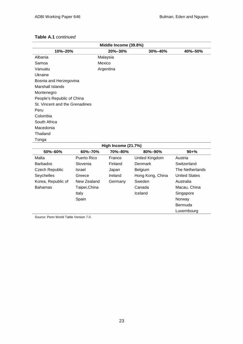
Table A.1 continued

Middle Income (39.8%) 10%–20% 20%–30% 30%–40% 40%–50%

Albania Malaysia Samoa Mexico Vanuatu Argentina Ukraine Bosnia and Herzegovina Marshall Islands Montenegro People’s Republic of China St. Vincent and the Grenadines Peru Colombia South Africa Macedonia Thailand Tonga

High Income (21.7%) 50%–60% 60%–70% 70%–80% 80%–90% 90+%

Malta Puerto Rico France United Kingdom Austria Barbados Slovenia Finland Denmark Switzerland Czech Republic Israel Japan Belgium The Netherlands Seychelles Greece Ireland Hong Kong, China United States Korea, Republic of New Zealand Germany Sweden Australia Bahamas Taipei,China Canada Macau, China Italy Iceland Singapore Spain Norway Bermuda Luxembourg Source: Penn World Table Version 7.0.


24

Figure A.1: Relative Income in 10-Year Increments, 1950–2009

Sources: Penn World Table Version 7.0; Authors’ calculations.

Figure A.1: The log of per capita income relative to the United States in time t is on the X axis, with the time t+10 value on the y axis. The dots correspond to every possible 10-year period between 1950 and 2009. The countries in orange are those that ever escape from middle to high income at any point. The orange countries in the middle-right quadrant (i.e., those that went from rich to middle and at some point also went from middle to rich) are the Czech Republic (which got rich in the mid-1990s after dropping to middle in 1990) and Lebanon (which got rich in the mid-1970s and then went to middle income in the early 1980s).

Figure A.2: Income Mobility at Different Income Categories

Sources: Penn World Table Version 7.0; Authors’ calculations.


25

Table A.2: Mean Value of Fundamentals for Middle-Income Escapees and Non-Escapees

All Middle-income 10%–20% of US 20%–30% of US

Non-escapees Escapees



Per capita GDP growth (%) 4.11 6.86 4.25 6.46 4.04 8.55 Total factor productivity (TFP) growth (%)

1.07 2.18 0.93 0.26 1.08 2.77

Average years of primary schooling relative to the US (%)

73.10 80.43 65.65 73.41 74.39 74.29

Average years of secondary schooling relative to the US (%)

31.00 43.10 28.46 33.72 32.01 45.94

Average years of tertiary schooling relative to the US (%)

17.20 22.46 14.71 21.99 18.04 23.11

Number of patents (1000) 1.79 6.97 2.26 1.33 1.53 1.44 Growth in agricultural share of GDP (%)

–2.68 –4.38 –2.20 –3.71 –3.00 –7.11

Growth in industry share of GDP (%) –0.04 1.79 0.21 3.56 –0.07 1.53 Growth in services share of GDP (%) 1.19 0.19 1.18 0.90 1.11 1.05 Exports as a share of GDP (%) 36.78 57.83 36.05 20.69 33.28 67.80 Log undervaluation 0.17 0.24 0.11 0.28 0.25 0.32 CPI inflation (%) 18.67 6.75 14.55 14.33 27.31 9.15 External debt as a share of GNI (%) 46.72 9.74 44.34 NA 41.11 NA Democracy indicator 5.02 3.81 4.16 1.21 5.27 2.51 Autocracy indicator 2.59 4.02 2.97 5.79 2.39 4.89 Gini coefficient 43.45 37.91 45.45 33.71 45.85 34.54 Age dependency ratio (%) 71.17 66.39 76.22 80.89 68.91 72.67 Change in Gini coefficient (%) 0.68 –0.32 0.76 0.47 0.58 –0.95 Change in age dependency ratio (%) –0.96 –1.62 –0.98 –0.84 –0.87 –1.80

30%–40% of US 40%–50% of US Non-escapees Escapees Non-escapees Escapees

Per capita GDP growth (%) 3.97 6.70 3.63 5.97 Total factor productivity (TFP) growth (%)

1.58 2.49 1.37 2.54

Average years of primary schooling relative to the US (%)

87.07 76.84 96.84 92.91

Average years of secondary schooling relative to the US (%)

30.99 46.89 43.11 44.78

Average years of tertiary schooling relative to the US (%)

19.61 20.33 26.62 23.84

Number of patents (1000) 1.77 3.42 0.50 12.21 Growth in agricultural share of GDP (%)

–2.90 –1.75 –4.30 –5.07

Growth in industry share of GDP (%) –0.49 1.46 –0.75 1.56 Growth in services share of GDP (%) 1.41 0.05 1.21 –0.20 Exports as a share of GDP (%) 41.46 63.92 49.33 61.34 Log undervaluation 0.22 0.24 0.13 0.17 CPI inflation (%) 18.96 4.69 6.91 4.89 External debt as a share of GNI (%) 41.92 8.00 62.98 10.17 Democracy indicator 6.27 4.19 8.17 6.32 Autocracy indicator 2.32 4.00 1.21 2.16 Gini coefficient 37.62 39.44 29.08 40.38 Age dependency ratio (%) 66.20 66.86 51.04 59.55 Change in Gini coefficient (%) 0.47 –0.13 0.99 –0.54 Change in age dependency ratio (%) –1.16 –2.81 –0.80 –1.31 CPI = consumer price index, GDP = gross domestic product, GNI = gross national income, US = United States. Note: Numbers in bold indicate significant difference at 95% confidence. Source: Authors’ calculations (see Data Appendix).


26

Table A.3: Main Regression Results (1) (2) (3) (4) (5)

Baseline Absolute

GDP No Lagged

Growth Low

Income Middle Income

Gini – concurrent average level –0.000 (1.03)

–0.000 (1.29)

–0.000 (0.58)

–0.000 (1.25)

–0.000 (2.40)*

Fertility – 5yr lag average 0.001 (0.54)

–0.000 (0.13)

0.001 (0.64)

0.000 (0.16)

0.003 (2.16)*

Dependency – concurrent avg change

–0.179 (0.98)

–0.124 (0.67)

–0.245 (1.22)

–0.121 (0.56)

–0.144 (0.83)

Agr./GDP – concurrent avg change

–0.321 (5.12)**

–0.312 (5.03)**

–0.378 (5.44)**

–0.329 (5.19)**

–0.181 (3.90)**

Tertiary – lag 1yr relative to US 0.001 (0.07)

0.001 (0.10)

–0.006 (0.51)

–0.005 (0.37)

0.005 (0.34)

CPI – 5yr lag average 0.000 (1.44)

0.000 (1.45)

0.000 (0.01)

0.000 (1.08)

0.000 (0.67)

Polity score – 5yr lag average 0.000 (1.45)

0.000 (1.36)

0.000 (1.12)

0.000 (1.36)

0.000 (1.76)

Trade/GDP – concurrent average level

–0.000 (0.86)

–0.000 (0.89)

–0.000 (1.10)

–0.000 (1.02)

0.000 (2.45)*

Log underval. – concurrent average level

0.004 (0.73)

0.004 (0.71)

0.004 (0.77)

0.003 (0.50)

–0.008 (1.41)

Variables Interacted with Middle-income Dummy

Gini – concurrent avg level –0.000 (1.24)

–0.000 (1.07)

–0.000 (1.56)

Fertility – 5yr lag avg 0.003 (1.37)

0.002 (1.25)

0.004 (1.80)

Dependency – concurrent avg change

0.009 (0.04)

0.019 (0.08)

–0.137 (0.49)

Agr/GDP – concurrent avg change

0.147 (1.94)

0.125 (1.66)

0.235 (2.89)**

Tertiary – lag 1yr relative to US 0.000 (0.02)

0.010 (0.56)

–0.003 (0.18)

CPI – 5yr lag avg –0.000 (0.88)

–0.000 (1.38)

–0.000 (2.07)*

Polity score – 5yr lag avg 0.000 (0.14)

0.000 (0.51)

0.000 (0.23)

Trade/GDP – concurrent avg level

0.000 (1.85)

0.000 (2.04)*

0.000 (2.04)*

Log underval. – concurrent avg level

–0.014 (1.78)

–0.016 (2.04)*

–0.022 (2.71)**

Controls Per capita GDP growth – 5yr lag avg

0.191 (6.06)**

0.190 (6.09)**

0.145 (3.03)**

0.220 (5.46)**

Per cap. GDP (rel. US unless specified)

–0.000 (2.19)*

–0.000 (4.70)**

–0.000 (0.74)

0.000 (0.17)

–0.000 (2.20)*

Constant 0.040 (4.77)**

0.049 (5.73)**

0.042 (4.63)**

0.045 (3.07)**

0.035 (3.55)**

Observations 1682 1682 1686 823 859 Sample L&M L&M L&M L M agr. = agricultural, avg = average, CPI = consumer price index, GDP = gross domestic product, L = low-income countries, M = middle-income countries, US = United States, yr = year. Notes: Robust z statistics in parentheses; * significant at the 5% level; ** significant at the 1% level. Source: Authors’ calculations (see Data Appendix for variable sources and definitions).


27

Table A.4: Growth with Different Structural Variables

Concurrent 10-year Growth of Agriculture Share of GDP Full Sample Low Income Middle Income

Variable -0.312 -0.320 -0.174 (4.25)** (4.18)** (4.97)** MI*Variable 0.127 (1.60) Lag 5yr avg growth 0.143 0.103 0.194 (4.25)** (2.08)* (7.61)** Income relative to US -0.000 (3.49)** Constant 0.037 0.036 0.028 (16.10)** (13.88)** (15.65)** Observations 3,898 2,116 1,782

Concurrent 10-year Growth of Industry Share of GDP Full Sample Low Income Middle Income

Variable 0.072 0.073 0.197 (1.48) (1.48) (4.53)** MI*Variable 0.124 (1.96)* Lag 5yr avg growth 0.154 0.144 0.165 (5.04)** (3.10)** (6.48)** Income relative to US -0.000 (1.21) Constant 0.036 0.036 0.033 (16.53)** (14.34)** (21.48)** Observations 3,893 2,111 1,782

Concurrent 10-year Growth of Services Share of GDP Full Sample Low Income Middle Income Variable 0.093 0.098 -0.156 (1.68) (1.78) (3.79)** MI*Variable -0.242 (3.57)** Lag 5yr avg growth 0.159 0.151 0.166 (5.07)** (3.13)** (6.53)** Income relative to US -0.000 (0.90) Constant 0.037 0.036 0.035 (16.65)** (14.07)** (21.85)** Observations 3,893 2,111 1,782 avg = average, GDP = gross domestic product, MI = middle income, US = United States, yr = year. Notes: Robust z statistics in parentheses; * significant at the 5% level; ** significant at the 1% level. Source: Authors’ calculations (see Data Appendix for variable sources and definitions).


28

Data Appendix Exclusion of Oil-rich Countries We identify oil-rich countries as those whose average oil exports, as a share of gross domestic product (GDP), exceed 30% or whose oil rents, as a share of GDP, exceed 29%, using World Bank World Development Indicators data. With these criteria, the oil exporters are Algeria, Angola, Azerbaijan, Bahrain, Brunei Darussalam, Chad, Congo, Equatorial Guinea, Gabon, Iran, Iraq, Kazakhstan, Kuwait, Libya, Nigeria, Oman, Qatar, Saudi Arabia, Trinidad and Tobago, Turkmenistan, United Arab Emirates, Venezuela, and Yemen.

International Growth Accounting Exercise Baseline data used for growth accounting exercise, including per capita GDP, employment, and investment, come from the Penn World Table Version 7.0 (Heston et al. 2011).

Following Caselli (2005), capital stocks are generated using a perpetual inventory method:

Kt = It + (1 − δ)Kt−1,

where It is investment and δ is the depreciation rate. We assume 6% depreciation across countries. For countries with available investment data pre-1970, we calculate the initial capital stock as

K0 = I0/(g + δ),

where I0 is investment in its first available year and g is the average geometric growth rate of investment between I0 and 1970. For those countries with investment data available starting only in the 1970s, we calculate Kt and K0 with the same equations, but substitute g as the average geometric growth rate of investment between I0 and 1980.

Human capital data at the primary, secondary, and tertiary levels come from Barro and Lee (2011). The data cover average years of schooling in the population over 15 years old from 1950 to 2010, in 5-year intervals.12 Given the persistence of years of schooling data, we extrapolate data for intervening years by assuming constant growth over each 5-year period. To generate a human capital index, we follow Hall and Jones (1999) and generate a human capital index as

h = eφ(s),

where s is average years of schooling and φ(s) is a piecewise linear function with slope contingent on estimates for returns to different levels of schooling: 0.13 for s ≤ 4, 0.10 for 4 < s ≤ 8, and 0.07 for 8 < s.13

12 With our focus on middle-income and lower-income countries, and given lower tertiary attendance rates

in these countries, we focus on years of schooling in the 15+ population rather than the 25+ population, as did Caselli (2005) and Hall and Jones (1999).

13 From Caselli (2005): “International data on education-wage profiles (Psacharopulos 1994) suggests that in Sub-Saharan Africa (which has the lowest levels of education) the return to one extra year of education is about 13.4 percent, the World average is 10.1 percent, and the OECD average is 6.8 percent. Hall and Jones’s measure tries to reconcile the log-linearity at the country level with the convexity across countries.”


29

In the baseline growth accounting exercise, we exclude human capital (its inclusion makes little difference, as shown below) and adopt a simple Cobb–Douglas production function:

Y = AKαL1-α,

Where Y is GDP, K is the aggregate capital stock, L is the number of workers, and α is a constant representing factor shares. We then divide through by the number of workers:

y = Akα,

where y = Y/L and k = K/L. A represents the efficiency with which capital and labor are used, and thus corresponds to total factor productivity (TFP). We take growth rates of y and k and then estimate TFP as

TFP = gy – α*gk,

where the prefix g denotes annual growth rates. In this equation, following general practice, we set α = 0.33. As a robustness check, we also calculate TFP including the human capital measure in the growth accounting exercise:14

y = Akαh1-α

The TFP results across income levels are not greatly affected by such a change.

Inequality Inequality data on Gini coefficients comes from Milanovic (2005). Milanovic calculates a variable “Giniall” that reports Gini coefficients from a wide range of nationally representative household surveys, covering 1,541 country/years. Given many missing observations and the relative annual persistence of Gini coefficients, we replace this “Giniall” variable by its running 5-year average.

Governance Governance indicators come from the Polity IV database. The democracy and autocracy indicators are composite variables (“DEMOC” and “AUTOC” in the original dataset) based on an additive 11-point scale (0–10). The included indicators for both composite variables can be found online (at http://www.systemicpeace.org/inscr/ p4manualv2010.pdf). The full “polity” score is calculated by subtracting a country’s autocracy value from its democracy value.

Undervaluation Undervaluation is calculated following Rodrik (2008), where a “real” exchange rate is calculated as the actual exchange rate divided by the purchasing power parity conversion factor, using the Penn World Table Version 7.0 data. Unlike Rodrik, this index is calculated on an annual, as opposed to 5-year, basis. Given the Balussa–Samuelson effect, whereby non-traded goods are cheaper in poorer countries, Rodrik generates estimated real exchange rates by regressing the log of the real exchange rate on log per capita GDP, including fixed effects for the time period. The undervaluation index is calculated as the difference between the log real exchange rate 14 Here, h is the human capital measure described earlier, and can be seen as the human capital per

worker; in other words, it is the “quality adjusted” workforce, Lh, divided by the number of workers.


30

and the fitted values from this regression (which correspond to the Balussa–Samuelson estimated real exchange rates). The undervaluation index is in log form, and positive values indicate higher levels of undervaluation.

Other Data Additional data come from the World Bank World Development Indicators dataset, and generally require no explanation. A full list of variables and data sources is presented in the table below for all variables whose calculation is not described.

Table DA.1: Variables and Sources

Variable Source GDP and GDP growth PWT Version 7.0 Employment PWT Version 7.0 Investment PWT Version 7.0 Years of schooling Barro and Lee (2011) Gini coefficient Milanovic (2005) Agriculture share of GDP World Bank Industry share of GDP World Bank Services share of GDP World Bank CPI inflation World Bank Patents World Bank Fertility World Bank Age dependency ratio World Bank Exports/GDP World Bank Trade/GDP PWT Version 7.0 Democracy indicator Polity IV Autocracy indicator Polity IV Polity score Polity IV

CPI = consumer price index, GDP = gross domestic product, PWT = Penn World Table. Source: Authors.

Asian Development Bank Institute · α = capital share, GDP = gross domestic product, K/L = capital...

Documents

Transcript of Asian Development Bank Institute · α = capital share, GDP = gross domestic product, K/L = capital...