ASecond-OrderEnergyStableBDFNumericalScheme for the …

Commun. Comput. Phys.doi: 10.4208/cicp.OA-2016-0197

Vol. 23, No. 2, pp. 572-602February 2018

A Second-Order Energy Stable BDF Numerical Scheme

for the Cahn-Hilliard Equation

Yue Yan1, Wenbin Chen1, Cheng Wang2,∗ and Steven M. Wise3

1 School of Mathematical Sciences, Fudan University, Shanghai 200433, China.2 Department of Mathematics, University of Massachusetts Dartmouth,North Dartmouth, MA 02747, USA.3 Mathematics Department, University of Tennessee, Knoxville, TN 37996, USA.

Received 9 November 2016; Accepted (in revised version) 2 May 2017

Abstract. In this paper we present a second order accurate (in time) energy stable nu-merical scheme for the Cahn-Hilliard (CH) equation, with a mixed finite element ap-proximation in space. Instead of the standard second order Crank-Nicolson method-ology, we apply the implicit backward differentiation formula (BDF) concept to derivesecond order temporal accuracy, but modified so that the concave diffusion term istreated explicitly. This explicit treatment for the concave part of the chemical potentialensures the unique solvability of the scheme without sacrificing energy stability. Anadditional term Aτ∆(uk+1−uk) is added, which represents a second order Douglas-Dupont-type regularization, and a careful calculation shows that energy stability is

guaranteed, provided the mild condition A≥ 116 is enforced. In turn, a uniform in time

H1 bound of the numerical solution becomes available. As a result, we are able toestablish an ℓ∞(0,T;L2) convergence analysis for the proposed fully discrete scheme,with full O(τ2+h2) accuracy. This convergence turns out to be unconditional; no scal-ing law is needed between the time step size τ and the spatial grid size h. A fewnumerical experiments are presented to conclude the article.

AMS subject classifications: 35K35, 35K55, 65M12, 65M60

Key words: Cahn-Hilliard equation, energy stable BDF, Douglas-Dupont regularization, mixedfinite element, energy stability.

1 Introduction

The Allen-Cahn (AC) [1] (non-conserved dynamics) and Cahn-Hilliard (CH) [7] (con-served dynamics) equations, which model spinodal decomposition in a binary alloy, are

∗Corresponding author. Email addresses: [email protected] (Y. Yan), [email protected] (W. Chen),[email protected] (C. Wang), [email protected] (S. M. Wise)

http://www.global-sci.com/ 572 c©2018 Global-Science Press

Y. Yan et al. / Commun. Comput. Phys., 23 (2018), pp. 572-602 573

perhaps the most well-known of the gradient flow-type PDEs. In deriving the CH equa-tion, we consider a bounded domain Ω⊂R

d (with d=2 or d=3). For any u∈H1(Ω), theCH energy functional is given by

E(u)=∫

Ω

(

1

4u4−

1

2u2+

ε2

2|∇u|2

)

dx, (1.1)

where ε is a positive constant that dictates the interface width. (See [7] for a detailedderivation.) The CH equation is precisely the H−1 (conserved) gradient flow of the en-ergy functional (1.1):

ut=∆w, in Ω×(0,T),

w :=δφE=u3−u−ε2∆u, in Ω×(0,T),

∂nu=∂nw=0, on ∂Ω×(0,T),

u(·,0)=u0, in Ω,

(1.2)

where T > 0 is the final time, which may be infinite; ∂nu := n·∇u; and n the unit nor-mal vector on the boundary. Due to the gradient structure of (1.2), the following energydissipation law holds:

d

dtE(u(t))=−

∫

Ω|∇w|2dx. (1.3)

In integral form, the energy decay may be expressed as

E(u(t1))+∫ t1

t0

∫

Ω|∇w(t)|2dxdt=E(u(t0)). (1.4)

Furthermore, the equation is mass conservative,∫

Ω∂tudx=0, which follows from the con-

servative structure of the equation together with the homogeneous Neumann boundaryconditions for w. This property can be re-expressed as (u(·,t),1)=(u0,1), for all t≥0.

The Cahn-Hilliard equation is one of the most important models in mathematicalphysics. It is often paired with equations that describe important physical behaviorof a given physical system, typically through nonlinear coupling terms. Examples ofsuch coupled models include the Cahn-Hilliard-Navier-Stokes (CHNS) equation for two-phase, immiscible flow; the Cahn-Larche model of binary solid state diffusion for elasticmisfit; the Cahn-Hilliard-Hele-Shaw (CHHS) equation for spinodal decomposition of abinary fluid in a Hele-Shaw cell; et cetera. The numerical and PDE analyses for the CHequation are quite challenging, since the equation is a fourth-order, nonlinear parabolic-type PDE. There have been many existing numerical works, in particular for first orderaccurate (in time) schemes.

Meanwhile, second order accurate (in time) numerical schemes have also attracted agreat deal of attention in recent years, due to the great advantage over their first ordercounterparts in terms of numerical efficiency and accuracy. However, the analysis forthe second order schemes is significantly more difficult than that for the first order ones,

574 Y. Yan et al. / Commun. Comput. Phys., 23 (2018), pp. 572-602

because of the more complicated form for the nonlinear terms; see the related discussionsin [2, 21, 24], et cetera.

The energy stability of a numerical scheme has been a very important issue, since itplays an essential role in the accuracy of long time numerical simulation. The standardconvex splitting scheme, popularized by Eyre’s work [17], is a well-known approach toachieve numerical energy stability. This framework treats the convex part of the chemicalpotential implicitly and the concave part explicitly, resulting in a scheme that is uniquelysolvable and energy stable, unconditionally with respect to the time and space step sizes.Splitting has been applied to a wide class of gradient flows in recent years, and both firstand second order accurate (in time) algorithms have been developed. See the relatedworks for the phase field crystal (PFC) equation and the modified phase field crystal(MPFC) equation [3,4,28,35,37]; epitaxial thin film growth models [8,10,32,34]; non-localCahn-Hilliard-type models [22,23]; the CHHS and related models [9,13,20,36]; et cetera.One drawback of the first order convex splitting approach, however, is that the extradissipation added to ensure unconditional stability also introduces a significant amountof numerical error [12]. For this reason, second-order energy stable methods have beenhighly desirable.

Recently, for the CH equation (1.2), a second order energy stable scheme has beenanalyzed in [25], based on a modified version of the Crank-Nicolson temporal approxi-mation; see the related discussions in Remarks 2.1 and 4.3. This numerical scheme enjoysmany advantages over the second order temporal approximations reported in the exist-ing literature [5, 16, 24, 38], in particular in terms of the unconditional energy stability,unconditionally unique solvability, and rigorous convergence properties. See also therecent finite element work [15] for related analysis; and see the extension of the ideasin [15, 25] to the Cahn-Hilliard-Navier-Stokes model in the recent papers [14, 27].

In this paper, we propose and analyze an alternate second order energy stable schemefor the CH equation (1.2), based on the 2nd order BDF temporal approximation frame-work, instead of that based on the Crank-Nicolson one. The BDF scheme treats and ap-proximates every term at the time step tn+1 (instead of the time instant tn+1/2). In moredetail, a 2nd order BDF 3-point stencil is applied in the temporal derivative approxima-tion, and the nonlinear term and the surface diffusion terms are updated implicitly, dueto their strong convexities. Meanwhile, a second order accurate, explicit extrapolationformula has to be applied in the approximation of the concave diffusion term, in order tomake the numerical scheme uniquely solvable.

However, the energy stability is not assured for this explicit extrapolation, by a directcalculation. To salvage the energy stability of the numerical scheme, we add a secondorder Douglas-Dupont regularization, in the form of Aτ∆(uk+1−uk). A more carefulanalysis then guarantees the energy stability for this proposed numerical scheme undera mild requirement A≥ 1

16 . For the present scheme, we highlight the fact that the nonlin-ear solver required for the BDF scheme is expected to require less computational effortthan that for the Crank-Nicolson version, due to the simpler form and stronger convexityproperties of the nonlinear term.


A mixed finite element approximation is taken in space, based on a mixed weak for-mulation of the CH equation (1.2). In this approach, the numerical solutions for both thephase variable u and the chemical potential variable w belong to the same finite elementspace Sh, which is a piecewise polynomial subspace of H1. Combined with the secondorder energy stable BDF temporal approximation, the resulting numerical scheme pre-serves the properties of unique solvability and unconditional energy stability. In turn,a uniform-in-time H1 bound can be derived for the numerical phase variable uh. Witha help of this uniform-in-time H1 bound, we are able to establish the convergence anal-ysis, with a combination of consistency and stability estimates for the numerical errorfunctions. The error estimate, in the ℓ∞(0,T;L2)∩ℓ2(0,T;H2

h) norm, has the full orderO(τ2+h2) accuracy. Furthermore, this convergence is unconditional; no scaling law isneeded between τ and h to ensure its validity.

This article is organized as follows. In Section 2 we outline the fully discrete scheme.The unique solvability is proven in Section 3 and the energy stability analysis is estab-lished in Section 4. In Section 5 we present the ℓ∞(0,T;L2)∩ℓ2(0,T;H2

h) convergence anal-ysis for the scheme. Some numerical results are presented in Section 6. Finally, conclud-ing remarks are given in Section 7.

2 The fully discrete numerical scheme

We use standard notation for the norms on their respective function spaces. In particular,we denote the standard norms for the Sobolev spaces Wm,p(Ω) by ‖·‖m,p. We replace‖·‖0,p by ‖·‖p, ‖·‖0,2 =‖·‖2 by ‖·‖, and ‖·‖q,2 by ‖·‖Hq .

The mixed weak formulation of Cahn-Hilliard equation (1.2) is to find u,w ∈L2(0,T;H1(Ω)), with ut∈L2(0,T;H−1(Ω)), satisfying

(ut,v)+(∇w,∇v)=0, ∀ v∈H1(Ω),

(w,ψ)=(u3−u,ψ)+ε2(∇u,∇ψ), ∀ ψ∈H1(Ω),(2.1)

for almost every t ∈ [0,T], where H−1(Ω) is the dual space of H1(Ω)∩L20(Ω), where

L20(Ω) :=

u∈L2(Ω)∣

∣ (u,1)=0

, and (·,·) represents the L2 inner product or the dual-ity pairing, as appropriate.

Let Th=K be a quasi-uniform triangulation on Ω. For q∈Z+, define the piecewise

polynomial space Sh :=v∈C0(Ω) |v|K ∈Pq(K),∀ K∈Th⊂H1(Ω).

We propose the following fully discrete numerical scheme: for n≥1, given un−1h ,un

h ∈

Sh, find un+1h ,wn+1

h ∈Sh, such that

(

3un+1h −4un

h+un−1h

2τ,vh

)

+(∇wn+1h ,∇vh)=0, ∀ vh ∈Sh,

(wn+1h ,ψh)= ε2(∇un+1

h ,∇ψh)+((un+1h )3−2un

h+un−1h ,ψh)

+Aτ(∇(un+1h −un

h),∇ψh), ∀ ψh ∈Sh,

(2.2)


where unh stands for the numerical solution at time tn. As a general rule, the second order

Gear method (BDF approximation) is expected to yield a large region of absolute stability.The explicit Adams-Bashforth extrapolation formula (with a second order approximationto the variable at time step tn+1) is applied to stabilize the concave term, as we will show.The artificial term Aτ∆(un+1

h −unh) – a second order-accurate Douglas-Dupont-type regu-

larization – is added to establish the unconditional energy stability of the scheme, providedA is sufficiently large, while preserving the second order temporal accuracy and uniquesolvability of the scheme. We will show that, there is only a very mild stability require-ment on the artificial parameter A, namely, A≥ 1

16 .The scheme requires an initialization step. To this end, we introduce the Ritz projec-

tion operator Rh : H1(Ω)→Sh, satisfying

(∇(Rh ϕ−ϕ),∇χ)=0, ∀χ∈Sh, (Rh ϕ−ϕ,1)=0. (2.3)

The initial data are chosen so that u0h =Rhu0. Then, we use a standard first-order energy

stable method to obtain u1h,w1

h ∈ Sh. Precisely, the initialization step is as follows: givenu0

h∈Sh, find u1h,w1

h∈Sh, such that

(

u1h−u0

h

τ,vh

)

+(∇w1h,∇vh)=0, ∀ vh ∈Sh,

(w1h,ψh)= ε2(∇u1

h,∇ψh)+((u1h)

3−u0h,ψh), ∀ ψh ∈Sh.

(2.4)

We must solve a nonlinear algebraic system at every time step in the computation.However, many nonlinear solvers, such as the Newton’s iteration or nonlinear conju-gate gradient algorithm, and the nonlinear multigrid give robust performance, since theimplicit part turns out to be the gradient of a certain strictly convex functional.

Remark 2.1. The Crank-Nicolson version of the second order convex splitting scheme forthe CH equation (1.2) takes the (spatially-continuous) form:

un+1−un

τ= ∆wn+1/2,

wn+1/2= χ(un+1,un)−

(

3

2un−

1

2un−1

)

−ε2∆

(

3

4un+1+

1

4un−1

)

,

χ(un+1,un) :=1

4(un+1+un)

(

(un+1)2+(un)2)

.

(2.5)

See the detailed derivations and analyses in [11, 15, 25], involving finite difference, finiteelement and Fourier pseudo-spectral discretizations, respectively. In this numerical ap-proach, every term in the chemical potential is approximated at the time instant tn+1/2:A modified implicit second order approximation is employed for the highest-order dif-fusion term in order to preserve a stronger stability than the standard Crank-Nicolsontreatment; a second order explicit extrapolation is employed for the concave term; and, a


modified Crank-Nicolson approximation (a secant approximation) is used on the nonlin-ear term.

We see that both the Crank-Nicolson version (2.5) and the BDF one (2.2) require anonlinear solver, while the nonlinear term in (2.5) takes a more complicated form than(2.2), which comes from different time instant approximations. Moreover, a stronger con-vexity of the nonlinear term in the BDF one (2.2) improves the numerical efficiency in thenonlinear iteration. In turn, the nonlinear iteration solver in the proposed scheme (2.2)is expected to incur less computational cost than that for (2.5). More detailed compari-son between these two different second order energy stable approaches will be given inRemarks 4.3, 4.4.

3 Unique solvability

To facilitate the analysis below, we define the discrete Laplacian operator and the dis-crete H−1 norm. We will make use of the notation L2

0(Ω) :=

u∈L2(Ω)∣

∣ (u,1)=0

, and,

generically, if V⊆ L2(Ω), V := L20∩V.

Definition 3.1. The discrete Laplacian operator ∆h :Sh→ Sh is defined as follows: for anyvh ∈Sh, ∆hvh ∈ Sh denotes the unique solution to the problem

(∆hvh,χ)=−(∇vh,∇χ), ∀ χ∈Sh.

It is straightforward to show that by restricting the domain, ∆h : Sh → Sh is invertible,and for any vh ∈ Sh, we have

(∇(−∆h)−1vh),∇χ)=(vh,χ), ∀ χ∈Sh.

Lemma 3.1. Let u∈H2N(Ω) :=

u∈H2(Ω)∣

∣ ∂nu=0 on ∂Ω

. Then

‖∆h(Rhu)‖≤‖∆u‖. (3.1)

Proof. Let vh ∈Sh be arbitrary. Then

−(∆u,vh)=(∇u,∇vh)=(∇(Rhu),∇vh)=−(∆h(Rhu),vh). (3.2)

Thus, setting vh =−∆h(Rhu), we have, by the Cauchy-Schwarz inequality,

‖∆h(Rhu)‖2=(∆u,∆h(Rhu))≤‖∆u‖·‖∆h(Rhu)‖. (3.3)

In turn, the result follows on dividing by ‖∆h(Rhu)‖.

Definition 3.2. The discrete H−1 norm, ‖·‖−1,h, is defined as follows:

‖vh‖−1,h :=√

(vh,(−∆h)−1vh), ∀vh ∈ Sh.


Now, suppose ψh ∈ Sh and take the test function as vh = (−∆h)−1ψh in our mixed

scheme (2.2), we obtain

(

3un+1h −4un

h+un−1h

2τ,(−∆h)

−1ψh

)

+ε2(∇un+1h ,∇ψh)

+((un+1h )3−2un

h+un−1h ,ψh)+Aτ(∇(un+1

h −unh),∇ψh)=0. (3.4)

By rearranging the above equation, we get, for every ψh ∈ Sh,

((un+1h )3−(Aτ+ε2)∆hun+1

h +3

2τ(−∆h)

−1(un+1h −u),ψh)= f [un

h ,un−1h ](ψh), (3.5)

where f [unh ,un−1

h ] is a bounded linear functional involving the previous time iterates and

u is the time-invariant mass average of ukh. We make the transformation qh=uk+1

h −u∈ Sh.

Then qh∈ Sh satisfies

((qh+u)3−(Aτ+ε2)∆hqh+3

2τ(−∆h)

−1qh,ψh)= f [unh ,un−1

h ](ψh), (3.6)

iff uk+1h ∈ Sh satisfies (3.5). Define

G(qh) :=1

4‖qh+u‖4

4+1

2(Aτ+ε2)‖∇qh‖

2+3

4τ‖qh‖

2−1,h− f [un

h ,un−1h ](qh).

Since G(·) is a strictly convex functional over the admissible set Sh, it has a unique mini-mizer. The unique minimizer, qh ∈ Sh, satisfies the Euler-Lagrange equation, which coin-cides with the variational problem (3.6). By equivalence, the solution to (3.4) exists andis unique. The unique solvability of the initialization scheme (2.4) is similar. See, forexample, [13].

4 Energy stability and a uniform-in-time H1 stability

The following energy stability estimate is available.

Theorem 4.1. For n≥1, define

E(un+1h ,un

h) :=E(un+1h )+

1

4τ‖un+1

h −unh‖

2−1,h+

1

2‖un+1

h −unh‖

2, (4.1)

and suppose A≥ 116 . Then the numerical scheme (2.2) has the energy-decay property

E(un+1h ,un

h)+τ

(

1−1

16A

)

∥

∥

∥

∥

∥

un+1h −un

h

τ

∥

∥

∥

∥

∥

2

−1,h

≤E(unh ,un−1

h ). (4.2)


Proof. In (2.2), taking vh=(−∆h)−1(un+1

h −unh) and ψh=un+1

h −unh , the two terms including

wh cancel out each other by the definition of ∆h. Therefore,

0=1

2τ(3un+1

h −4unh+un−1

h ,−∆−1h (un+1

h −unh))+ε2(∇un+1

h ,∇(un+1h −un

h))

+((un+1h )3,un+1

h −unh)−(2un

h−un−1h ,un+1

h −unh)+Aτ‖∇(un+1

h −unh)‖

2

:= J1+ J2+ J3+ J4+ J5.

We establish now establish estimates for J1,··· , J5. The time difference term becomes

J1=1

2τ(3un+1

h −4unh+un−1

h ,−∆−1h (un+1

h −unh))

= τ

5

4

∥

∥

∥

∥

∥

un+1h −un

h

τ

∥

∥

∥

∥

∥

2

−1,h

−1

4

∥

∥

∥

∥

∥

unh−un−1

h

τ

∥

∥

∥

∥

∥

2

−1,h

+τ3

4

∥

∥

∥

∥

∥

un+1h −2un

h+un−1h

τ2

∥

∥

∥

∥

∥

2

−1,h

. (4.3)

The highest-order diffusion term turns out to be

J2= ε2(∇un+1h ,∇(un+1

h −unh))

=ε2

2

(

‖∇un+1h ‖2−‖∇un

h‖2)

+ε2

2

∥

∥

∥∇(un+1

h −unh)∥

∥

∥

2. (4.4)

For the nonlinear term, we have

J3 =((un+1h )3,un+1

h −unh)=

1

4

(

‖un+1h ‖4

L4 −‖unh‖

4L4

)

+1

4

∥

∥

∥(un+1

h )2−(unh)

2∥

∥

∥

2

+1

2

∥

∥

∥un+1h (un+1

h −unh)∥

∥

∥

2. (4.5)

For the concave diffusive term, we have

J4= −(2unh−un−1

h ,un+1h −un

h)=−(unh ,un+1

h −unh)−(un

h−un−1h ,un+1

h −unh)

= −1

2

(

‖un+1h ‖2−‖un

h‖2)

+1

2‖un+1

h −unh‖

2

+(un+1h −2un

h+un−1h ,un+1

h −unh)−

∥

∥

∥un+1

h −unh

∥

∥

∥

2

= −1

2‖un+1

h ‖2+1

2

∥

∥

∥un+1

h −unh

∥

∥

∥

2−

(

−1

2‖un

h‖2+

1

2

∥

∥

∥un

h−un−1h

∥

∥

∥

2)

+1

2

∥

∥

∥un+1h −2un

h+un−1h

∥

∥

∥

2−

1

2

∥

∥

∥un+1h −un

h

∥

∥

∥

2. (4.6)

Finally, for the stabilizing term, we have

J5=Aτ‖∇(un+1h −un

h)‖2.


Using the Cauchy-Schwarz inequality, for any α>0,

1

2‖un+1

h −unh‖

2≤1

2

∥

∥

∥∇un+1

h −∇unh

∥

∥

∥·‖un+1

h −unh‖−1,h

≤τ

4α

∥

∥

∥∇un+1

h −∇unh

∥

∥

∥

2+

ατ

4

∥

∥

∥

∥

∥

un+1h −un

h

τ

∥

∥

∥

∥

∥

2

−1,h

. (4.7)

Putting everything together, we have

E(un+1h ,un

h)+τ(

1−α

4

)

∥

∥

∥

∥

∥

un+1h −un

h

τ

∥

∥

∥

∥

∥

2

−1,h

+τ

(

A−1

4α

)

‖∇(un+1h −un

h)‖2≤E(un

h ,un−1h ),

where the numerical energy function E(un+1h ,un

h) is defined in (4.1). The result follows on

setting α= 14A .

We have the following well-known stability for the initialization scheme.

Theorem 4.2. The initialization scheme (2.4) has the energy-decay property

E(u1h)+τ

∥

∥

∥

∥

∥

u1h−u0

h

τ

∥

∥

∥

∥

∥

2

−1,h

≤E(u0h). (4.8)

Since∥

∥

∥

u1h−u0

hτ

∥

∥

∥

−1,h=∥

∥∇w1h

∥

∥, this is equivalent to

E(u1h)+τ

∥

∥

∥∇w1h

∥

∥

∥

2≤E(u0

h). (4.9)

Remark 4.1. A requirement for the artificial coefficient, A≥ 116 , ensures a modified energy

stability at a theoretical level. On the other hand, this requirement may be more associ-ated with theoretical justification than practical necessity. Several numerical experimentshave shown that the non-increasing energy property is still observed even with a valueof A<

116 ; see the detailed numerical simulation results reported in Section 6.

Remark 4.2. Due to the forms of the energy (1.1) and the dynamical equation (1.2), thelower bound requirement for A is ε-independent: A ≥ 1

16 . Meanwhile, if the tempo-ral scale is multiplied by an ε−1 factor, so that the energy functional becomes E(u) =ε−1( 1

4‖u‖4L4 −

12‖u‖2)+ ε

2‖∇u‖2, as analyzed in [19, 33], a careful calculation indicates an

ε-dependent requirement: A≥ 116 ε−2, to ensure a modified energy stability in a similar

form as (4.2).


Remark 4.3. The Crank-Nicolson scheme (2.5), reported in [11, 15, 25], has also beenproven to be uniquely solvable and unconditionally energy stable, combined with ei-ther the finite difference or mixed finite element spatial approximation. In particular, itis observed that no additional regularization term is needed for this scheme, in contrastwith the proposed BDF scheme (2.2). The reason for this difference comes from the subtlefact that the explicit treatment for the concave term in (2.5), namely 3

2 un− 12 un−1 (a second

order approximation to u at tn+1/2), leads to the following stability estimate:

(−3

2un+

1

2un−1,un+1−un)≥ −

1

2(‖un+1‖2−‖un‖2)

+1

4(‖un+1−un‖2−‖un−un−1‖2). (4.10)

In contrast, equality (4.6) (for the BDF scheme) contains a negative term in the energy esti-mate: − 1

2‖unh−un−1

h ‖2. Consequently, an artificial term associated with Douglas-Dupontregularization is needed to balance this negative part, in order to establish the energystability at a theoretical level.

Remark 4.4. We have performed a numerical test to justify the expected improvement innumerical efficiency of the proposed BDF scheme (2.2), with respect to the energy stableCrank-Nicolson scheme (2.5), as argued in Remark 2.1. An exact numerical solution isset over a domain Ω=(0,1)2, with the physical parameter ε=0.05, the spatial resolutionh = 1

512 , and time step size τ = 0.01. The preconditioned steepest descent (PSD) algo-rithm, proposed and analyzed in a more recent article [18], is applied to implement bothnumerical schemes, with the same initial guess in the nonlinear iterations.

This numerical comparison is performed on an Apple iMac computer, with an In-tel Core i6, 2.9 GHz processor, and 32 GB of 1600 MHz DDR3 memory. Our numericalexperiments show that, it took 11 iterations for the BDF scheme (2.2) to obtain an errortolerance of 10−12 (in the maximum norm), with 0.4042 seconds CPU time, while theCrank-Nicolson version (2.5) requires 14 iterations to obtain the same level of error toler-ance, with 0.5263 seconds CPU time. As a result, we conclude that, since the nonlinearterm in (2.2) has a stronger convexity than the one in (2.5), a 20 to 25 percent improvementof the computational efficiency is generally expected.

In addition to the proposed BDF scheme in this article and the Crank-Nicolson ver-sion [11, 14, 15, 25], there are a few related works with second-order in time approxima-tions for the CH equation that we like to mention. A combination of an implicit midpointrule and spatial discretization by the Fourier-Galerkin spectral method was introducedin a recent article [5]; the stability estimates proved may be viewed as conditional, thereis a stability condition for τ in terms of the model parameters, although this restrictiondoes not depend on h.

A semi-discrete second-order scheme for a family of Cahn-Hilliard-type equationswas proposed in [38], with applications to diffuse interface tumor growth models. Anunconditional energy stability was proved, by taking advantage of a (quadratic) cut-off


of the double-well energy and artificial stabilization terms. And also, their scheme turnsout to be linear, which is another advantage. However, a convergence analysis is notavailable in their work.

A careful examination of several second-order in time numerical schemes for the CHequation is presented in [24]. An alternate variable is used in the numerical design, de-noted as a second order approximation to v=u2−1. A linearized, second order accuratescheme is derived as the outcome of this idea, and an unconditional energy stability isestablished in a modified version. However, such an energy stability is applied to a pairof numerical variables (u,v), and an H1 stability for the original physical variable u hasnot been justified. As a result, the convergence analysis is not available for this numericalapproach. Similar methodology has been reported in the invariant energy quadratization(IEQ) approach [26, 39–41].

By combining all these observations, we note many advantages of the proposed BDFscheme and the Crank-Nicolson version over the second order temporal approximationsreported in the existing literature, in particular in terms of the unconditional energy sta-bility, unconditionally unique solvability and convergence analysis.

Remark 4.5. As an alternative to the nonlinear approaches, there has been a recent workof a linear BDF-type scheme in [30]:

3un+1−4un+un−1

2τ=∆(

2(un)3−(un−1)3−(2un−un−1)−ε2∆un+1)

−Aτ(−∆)α(un+1−un), with α=0 or 1. (4.11)

The most important difference with our proposed BDF scheme (2.2) is the purely ex-plicit treatment for the nonlinear part of chemical potential, which in turn avoids anonlinear solver. However, with this explicit update for the nonlinear term, a theoret-ical justification of the energy stability for (4.11) requires a coefficient A of the orderA =O(ε−36|logε|16) for α = 0, and A =O(ε−26|logε|12) for α = 1. Also see the relatedanalysis for the first order linear scheme [31]. In comparison, our proposed algorithm(2.2) only requires A≥ 1

16 for the energy stability.

Since the nonlinear part of the chemical potential (un+1)3 appears as a convex termin (2.2), either the nonlinear multigrid or Newton’s iteration could be efficiently applied,and extensive numerical experiments have indicated a comparable computation cost asthat for (4.11).

As a result of the stability estimate (4.2) for the numerical energy function (4.1), weare able to obtain an uniform-in-time H1 estimate of the numerical solution:

Theorem 4.3. Suppose that the initial data are sufficiently regular that

E(u0h)+

1

3

∥

∥u0h

∥

∥

2≤

C0

3,


for some C0 that is independent of h, and A≥ 116 . Define κA :=1− 1

16A and wn+1h :=∆−1

h

( un+1h −un

hτ

)

,for n≥ 0. Then, there are constants C1,C2,C3 > 0, which depend on C0, Ω, and ε, but are inde-pendent of h and τ, such that for any m≥1

‖umh ‖

2H1 ≤ C1, (4.12)

τ ·κA

m

∑n=1

∥

∥

∥

∥

∥

unh−un−1

h

τ

∥

∥

∥

∥

∥

2

−1,h

=τ ·κA

m

∑n=1

‖∇wnh‖

2≤ C2, (4.13)

τ ·κA

m

∑n=1

‖∇wnh‖

2≤ C3. (4.14)

Proof. Since, for any u∈L4(Ω), 14 ‖u‖4

L4− 12 ‖u‖2≥ 1

2 ‖u‖2−|Ω|, it follows that

1

2‖un

h‖2+

ε2

2‖∇un

h‖2≤E(un

h)+|Ω|,

for any n ≥ 0. From the stability of the initialization step (4.8) and using the triangleinequality, we have

E(u1h,u0

h)= E(u1h)+

1

4τ‖u1

h−u0h‖

2−1,h+

1

2‖u1

h−u0h‖

2

≤ E(u1h)+

1

τ‖u1

h−u0h‖

2−1,h+

1

2‖u1

h−u0h‖

2

≤ E(u0h)+

∥

∥

∥u1

h

∥

∥

∥

2+∥

∥u0h

∥

∥

2

≤ E(u0h)+2E(u1

h)+2|Ω|+∥

∥u0h

∥

∥

2

≤ 3E(u0h)+

∥

∥u0h

∥

∥

2+2|Ω|≤C0+2|Ω|. (4.15)

By definition,

∥

∥

∥

∥

un+1h −un

hτ

∥

∥

∥

∥

−1,h

=∥

∥

∥∇wn+1h

∥

∥

∥, and the energy stability reads

E(un+1h ,un

h)+τ ·κA

∥

∥

∥∇wn+1h

∥

∥

∥

2≤E(un

h ,un−1h ), n≥1.

Therefore, for any m≥2,

E(umh )≤E(um

h ,um−1h )+τ ·κA

m

∑n=2

‖∇wnh‖

2≤E(u1h,u0

h)≤C0+2|Ω|. (4.16)

It follows that, for any m≥0

‖umh ‖

2H1 ≤

2(C0+3|Ω|)

ε2=: C1,


assuming that ε≤1. Next, using the stability (4.9) and the fact that ∇w1h=∇w1

h, we have,for any m≥1,

τ ·κA

m

∑n=1

∥

∥

∥

∥

∥

unh−un−1

h

τ

∥

∥

∥

∥

∥

2

−1,h

=τ ·κA

m

∑n=1

‖∇wnh‖

2≤4C0

3+2|Ω|=: C2.

Finally, for some time varying mass parameter αn ∈R,

wnh =αn+

32 wn

h−12 wn−1

h , n≥2,

w1h, n=1,

which implies that∥

∥∇wnh

∥

∥≤2∥

∥∇wnh

∥

∥. We can conclude that

τ ·κA

m

∑n=1

‖∇wnh‖

2≤4C2=: C3,

and the proof is complete.

5 Convergence analysis and error estimate

We denote the exact solution as un =u(x,tn) at t= tn . As usual, a regularity assumptionhas to be made in the error analysis, and we denote all the upper bounds for the exactsolution as C0. The following estimates hold for Ritz projection [6]:

‖Rh ϕ‖1,p≤C‖ϕ‖1,p, ∀1< p≤∞, (5.1)

‖ϕ−Rh ϕ‖p+h‖ϕ−Rh ϕ‖1,p≤Chq+1‖ϕ‖q+1,p, ∀1< p≤∞. (5.2)

Suppose that u∈L∞(0,T;W1,p). Combining (5.1) and the Sobolev imbedding theorem:W1,p(Ω) → L∞(Ω), for 2< p≤∞ (d= 2), 3< p≤∞ (d= 3), there are constants C4,C5 > 0such that

‖un‖∞ ≤C‖un‖1,p≤C4,

‖Rhun‖∞ ≤C‖Rhun‖1,p≤C‖un‖1,p≤C5.

The following discrete Gronwall inequality is needed in the error analysis.

Lemma 5.1. For a fixed T = τ ·N, where N is a positive integer, and τ > 0, assume thatanN

n=1,bnNn=1 and cnN−1

n=1 are all non-negative sequences, with τ∑N−1n=1 cn≤C6, where C6>0

is independent of τ and N, but possibly dependent on T. If for all τ > 0, there is some C7 > 0,which is independent of τ and N, such that

aN+τN

∑n=1

bn ≤C7+τN−1

∑n=1

ancn,


then

aN+τN

∑n=1

bn ≤ (C7+τa0c0)exp

(

τN−1

∑n=1

cn

)

≤ (C7+τa0c0)exp(C6).

Before proceeding into the convergence analysis, we introduce a new norm. Let Ω be

an arbitrary bounded domain and p= [u,v]T ∈[

L2(Ω)]2

. We define the G-norm to be aweighted inner product

‖p‖2G=(p,Gp), G=

[

12 −1

−1 52

]

.

Since G is symmetric positive definite, the norm is well-defined. Moreover,

G=

[

12 −1

−1 52

]

=

[

12 −1

−1 2

]

+

[

0 0

0 12

]

=:G1+G2.

By the positive semi-definiteness of G1, we immediately have

‖p‖2G=(p,(G1+G2)p)≥ (p,G2p)=

1

2‖v‖2. (5.3)

In addition, for any vi ∈L2(Ω),i=0,1,2, the following equality is valid:

(

3

2v2−2v1+

1

2v0,v2

)

=1

2(‖p2‖

2G−‖p1‖

2G)+

‖v2−2v1+v0‖2

4, (5.4)

with p1=[v0,v1]T,p2=[v1,v2]T.

By (u,w) we denote the exact solution to the original CH equation (1.2). We say thatthe solution pair of regularity of class C if and only if

u∈ W3,∞(0,T;L2)∩W1,∞(0,T;Hq+1), (5.5)

w∈ L2(0,T;Hq+1). (5.6)

The following theorem is the main result of this section.

Theorem 5.1. Suppose that the exact solution pair (u,w) is in the regularity class C, for the fixedfinal time T>0. Let un=u(tn) and un

h be the solution at time t=tn to the fully discrete numericalscheme (2.2), for 1≤n≤N, with N ·τ=T. Then we have the error estimate

‖un−unh‖+

(

τε2n

∑k=1

‖∆h(Rhuk−ukh)‖

2

)1/2

≤C8(hq+1+τ2), (5.7)

for some constant C8>0 that is independent of τ and h.


Proof. First we define error functions: enu := un−un

h , enw := wn−wn

h . Then the followingequations for the error functions hold: for any vh,ψh∈Sh,

(

δτen+1u ,vh

)

+(∇en+1w ,∇vh)=−

(

Rn+11 ,vh

)

, (5.8)

ε2(∇en+1u ,∇ψh)−(en+1

w ,ψh)+τ(∇Tn+12 ,∇ψh)=(Tn+1

1 −Tn+13 ,ψh)

+(Rn+12 −Rn+1

3 ,ψh), (5.9)

where

δτvn+1 :=

3vn+1−4vn+vn−1

2τ , n≥1,

v1−v0

τ , n=0,(5.10)

Rn+11 := un+1

t −δτun+1, (5.11)

Rn+12 := un+1−

2un−un−1, n≥1,

u0, n=0,(5.12)

Rn+13 :=

Aτ∆(un+1−un), n≥1,

0, n=0,(5.13)

Tn+11 :=

2enu−en−1

u , n≥1,

e0u, n=0,

(5.14)

Tn+12 :=

A(en+1u −en

u), n≥1,

0, n=0,(5.15)

Tn+13 := (un+1)3−(un+1

h )3. (5.16)

By the Cauchy-Schwarz inequality, we have the following estimate

‖Rn+11 ‖2≤

32τ3∫ tn+1

tn−1‖∂tttu‖2dt, n≥1,

τ3

∫ t1

0 ‖∂ttu‖2 dt, n=0

≤

32τ3∫ tn+1


τ2

3 ‖u‖W2,∞(0,T;L2) , n=0

≤

32τ3∫ tn+1


C9τ2, n=0.(5.17)

An analogous estimate is available for the second remainder term: for the case n≥1, wehave

‖Rn+12 ‖2≤32τ3

∫ tn+1

tn−1

‖∂ttu‖2dt.


We will not directly need an estimate of∥

∥R12

∥

∥, but we will address the control of R12

shortly. For the third remainder term, we obtain the estimate

‖Rn+13 ‖2≤

A2τ3∫ tn+1

tn‖∂t∆u‖2dt, n≥1,

0, n=0.

Suppose vh ∈Sh is arbitrary. Using the definitions of Ritz projection and the discreteLaplacian, ∆h, we have

(∇en+1w ,∇vh)=(∇wn+1−∇Rhwn+1,∇vh)+(∇Rhwn+1−∇wn+1

h ,∇vh)

=(∇(Rhwn+1−wn+1h ),∇vh)

=(Rhwn+1−wn+1h ,−∆hvh)

=(wn+1−wn+1h +Rhwn+1−wn+1,−∆hvh)

=(en+1w ,−∆hvh)−(wn+1−Rhwn+1,−∆hvh).

Combining the last equation with the error equations (5.9) and (5.8), and taking ψh =−∆hvh, yields

(

δτen+1u ,vh

)

+τ(∇Tn+12 ,∇(−∆h)vh)+ε2(∇en+1

u ,∇(−∆h)vh)

=−(Rn+11 ,vh)+(Tn+1

1 −Tn+13 ,−∆hvh)

+(Rn+12 −Rn+1

3 ,−∆hvh)+(wn+1−Rhwn+1,−∆hvh).

Denote ρn+1:=un+1−Rhun+1 and σn+1h :=Rhun+1−un+1

h , then we get en+1u =ρn+1+σn+1

h .By the definition (2.3) of Ritz projection, it holds that (∇ρn+1,∇χ) = 0, for all χ ∈ Sh.Therefore, with vh =σn+1

h , the error equation can be written as follows:(

δτσn+1h ,σn+1

h

)

+ǫ2‖∆hσn+1h ‖2+τ(∇Tn+1

2,h ,∇(−∆h)σn+1h )

= −(Rn+11 ,σn+1

h )−(Tn+13 ,−∆hσn+1

h )+(Tn+11,a ,−∆hσn+1

h )

+(Tn+11,h ,−∆hσn+1

h )+(Rn+12 ,−∆hσn+1

h )−(Rn+13 ,−∆hσn+1

h )

+(wn+1−Rhwn+1,−∆hσn+1h )−(δτρn+1,σn+1

h )

= : J1+ J2+ J3+ J4+ J5+ J6+ J7+ J8=: J, (5.18)

where

Tn+11,a :=

2ρn−ρn−1, n≥1,

ρ0, n=0,(5.19)

Tn+11,h :=

2σnh −σn−1

h , n≥1,

σ0h ≡0, n=0,

(5.20)

Tn+12,h :=

A(σn+1h −σn

h ), n≥1,

0, n=0.(5.21)


Observe that σ0h ≡0, because of our choice of initial data.

Now look at the left-hand side of (5.18). From (5.4), we have

(

δτσn+1h ,σn+1

h

)

=

12τ (‖pn+1‖2

G−‖pn‖2

G)+ 1

4τ‖σn+1h −2σn

h +σn−1h ‖2, n≥1,

12τ (‖σ1

h‖2−‖σ0

h‖2)+ 1

2τ‖σ1h −σ0

h‖2, n=0,

(5.22)

where pk+1=[σkh ,σk+1

h ]T. Using the definition of ∆h, it follows that

τ(∇Tn+12,h ,∇(−∆h)σ

n+1h )=Aτ(−∆hσn+1

h +∆hσnh ,−∆hσn+1

h )

≥1

2Aτ(‖∆hσn+1

h ‖2−‖∆hσnh ‖

2).

As a result, the left-hand side of (5.18) is bounded from below: for n≥1,

1

2τ

(

‖pn+1‖2G−‖pn‖2

G

)

+1

2Aτ(

‖∆hσn+1h ‖2−‖∆hσn

h ‖2)

+ǫ2‖∆hσn+1h ‖2≤ J,

and, for n=0,1

2τ‖σ1

h‖2+ǫ2‖∆hσ1

h‖2≤ J.

Now we study the seven terms on the right-hand side of (5.18).

J1= (−Rn+11 ,σn+1

h )≤‖Rn+11 ‖·‖σn+1

h ‖

≤

32τ3∫ tn+1

tn−1‖∂tttu‖2dt+ 1

4‖σn+1h ‖2, n≥1,

2C9τ3+ 18τ‖σ1

h‖2, n=0.

For J8, we have

J8=−(

δτρn+1,σn+1h

)

≤∥

∥

∥δτρn+1

∥

∥

∥

2+

1

4‖σn+1

h ‖2.

In addition, (5.2) indicates that

∥

∥

∥δτρn+1∥

∥

∥

2=∥

∥

∥(I−Rh)δτun+1∥

∥

∥

2

≤

9Ch2(q+1)

2τ

∫ tn+1

tn−1‖∂tu‖2

Hq+1dt, n≥1,

Ch2(q+1)

τ

∫ t1

0 ‖∂tu‖2Hq+1 dt, n=0,

which, in turn, shows that, for all 0≤n≤N−1,

J8≤

9Ch2(q+1)

2τ

∫ tn+1

tn−1‖∂tu‖2

Hq+1dt+ 14‖σn+1

h ‖2, n≥1,

Ch2(q+1)

τ

∫ t1

0 ‖∂tu‖2Hq+1dt+ 1

4‖σ1h‖

2, n=0.


For J5, we estimate the n=0 and n≥1 cases separately. For n≥1,

J5 = (Rn+12 ,−∆hσn+1

h )≤4

ε232τ3

∫ tn+1

tn−1

‖∂ttu‖2dt+

ε2

16‖∆hσn+1

h ‖2. (5.23)

To facilitate the special analysis for the initialization step, we need a more careful ap-proach. For n=0, we proceed as follows: using the definition of the Ritz projection, thediscrete Laplacian, and the stability (3.1),

J5 = (R12,−∆hσ1

h )=(ρ1−ρ0,−∆hσ1h )+(Rh(u

1−u0),−∆hσ1h )

= (ρ1−ρ0,−∆hσ1h )−(∆h(Rh(u

1−u0)),σ1h )

≤∥

∥

∥ρ1−ρ0

∥

∥

∥·∥

∥

∥∆hσ1

h

∥

∥

∥+∥

∥

∥∆h(Rh(u

1−u0))∥

∥

∥·∥

∥

∥σ1

h

∥

∥

∥

≤∥

∥

∥ρ1−ρ0∥

∥

∥·∥

∥

∥∆hσ1h

∥

∥

∥+∥

∥

∥∆(u1−u0)∥

∥

∥·∥

∥

∥σ1h

∥

∥

∥

≤2

ε2

Ch2(q+1)

τ

∫ t1

0‖∂tu‖

2Hq+1dt+

ε2

8‖∆hσ1

h‖2

+2C10τ3+1

8τ‖σ1

h‖2. (5.24)

Here we have made use of the estimate

∥

∥

∥∆(u1−u0)

∥

∥

∥

2≤τ

∫ t1

0‖∂t∆u‖2 dt≤τ2‖u‖W1,∞(0,T;H2)≤C10τ2.

For J6, we have

J6≤ ‖Rn+13 ‖·‖∆hσn+1

h ‖2

≤

4ε2 A2τ3

∫ tn+1

tn‖∂t∆u‖2dt+ ε2

16‖∆hσn+1h ‖2, n≥1,

0, n=0.(5.25)

For J7 and J3, we have, using the standard finite element approximations,

J7 =((I−Rh)wn+1,−∆hσn+1

h )≤2Ch2(q+1)

ε2‖wn+1‖2

Hq+1+ε2

8‖∆hσn+1

h ‖2, (5.26)

and

J3= (Tn+11,a ,−∆hσn+1

h )

≤2

ε2‖Tn+1

1,a ‖2+ε2

8‖∆hσn+1

h ‖2

≤ε2

8‖∆hσn+1

h ‖2+4Ch2(q+1)

ε2

4‖un‖2Hq+1+‖un−1‖2

Hq+1 , n≥1,

‖u0‖2Hq+1 , n=0.

(5.27)


For J4,

J4= (Tn+11,h ,−∆hσn+1

h )

≤2

ε2‖Tn+1

1,h ‖2+ε2

8‖∆hσn+1

h ‖2

≤ε2

8‖∆hσn+1

h ‖2+4

ε2

4‖σnh ‖

2+‖σn−1h ‖2, n≥1,

0, n=0.(5.28)

The analysis of the nonlinear term is given by (5.32) in Proposition 5.1:

J2≤2C11h2(q+1)

ε2‖un+1‖2

Hq+1+54

ε6C4

12‖σn+1h ‖2+

ε2

4‖∆hσn+1

h ‖2.

Substituting these terms into (5.18), and multiplying by 2τ on both sides, we have, forn≥1,

‖pn+1‖2G−‖pn‖2

G+Aτ2(‖∆hσn+1h ‖2−‖∆hσn

h ‖2)+

τε2

2‖∆hσn+1

h ‖2

≤

(

1+108

ε6C4

12

)

τ‖σn+1h ‖2+

32τ

ε2‖σn

h ‖2+

8τ

ε2‖σn−1

h ‖2

+9Ch2(q+1)∫ tn+1

tn−1

‖∂tu‖2Hq+1dt+

4Ch2(q+1)

ε2τ‖wn+1‖2

Hq+1

+4

ε2C11τh2(q+1)‖un+1‖2

Hq+1+32C

ε2τh2(q+1)‖un‖2

Hq+1

+8C

ε2τh2(q+1)‖un−1‖2

Hq+1+64τ4∫ tn+1

tn−1

‖∂tttu‖2dt

+8

ε2τ4

(

32∫ tn+1

tn−1

‖∂ttu‖2dt+A2

∫ tn+1

tn

‖∂t∆u‖2dt

)

. (5.29)

For n=0, we have a similar form:

‖σ1h‖

2+2τε2‖∆hσ1h‖

2

≤

(

τ

2+

1

2+

108τ

ε6C4

12

)

‖σ1h‖

2+3τε2

2‖∆hσ1

h‖2+2Ch2(q+1)

∫ t1

0‖∂tu‖

2Hq+1 dt

+4Ch2(q+1)

ε2τ‖w1‖2

Hq+1+4

ε2C11τh2(q+1)‖u1‖2

Hq+1

+8C

ε2τh2(q+1)‖u0‖2

Hq+1+4

ε2Ch2(q+1)

∫ t1

0‖∂tu‖

2Hq+1dt+4τ4C9+4τ4C10. (5.30)

With the help of Proposition 5.2, we get

‖σn+1h ‖+

(

τε2n+1

∑k=1

‖∆hσkh‖

2

)1/2

≤CT,ε(hq+1+τ2), (5.31)


with CT,ε independent of τ and h. In addition, it is easy to see from (5.2) that

‖ρk‖≤Chq+1‖uk‖Hq+1 , 1≤ k≤n+1.

Together with the triangle inequality ‖en+1u ‖≤ ‖ρn+1‖+‖σn+1

h ‖, we finally arrive at theconclusion of the theorem.

The following two propositions are used in the convergence analysis; their proofs aregiven in the Appendix.

Proposition 5.1. For the nonlinear error inner product term J2, as given by (5.18), wehave

J2 ≤2C11h2(q+1)

ε2‖un+1‖2

Hq+1+54

ε6C4

12‖σn+1h ‖2+

ε2

4‖∆hσn+1

h ‖2. (5.32)

Proposition 5.2. By the error evolution inequalities (5.29), (5.30), the following conver-gence estimate is valid:

‖σn+1h ‖+

(

τε2n+1

∑k=1

‖∆hσkh‖

2

)1/2

≤CT,ε(hq+1+τ2), (5.33)

with CT,ε independent of τ and h, under a technical assumption

0<τ≤1

4

(

1+108

ε6C4

12

)−1

:=τ1. (5.34)

Remark 5.1. We note that the ℓ∞(0,T;L2)∩ℓ2(0,T;H2h) convergence (5.7) is unconditional

in the following sense: there is no restriction for τ in terms of h to guarantee convergence.In fact, the energy stability estimate (given by Theorem 4.1) plays an essential role in thederivation of this unconditional convergence analysis. Specifically, the uniform-in-timeH1 estimate (4.12), a direct consequence of (4.2), leads to an ℓ∞(0,T;L6) bound of the nu-merical solution. As a result, the nonlinear coefficients are bounded in the estimate (A.2),and we only need to handle the L6 and discrete H2 norms of the projection error func-tion. This could be accomplished via repeated applications of 3-D Sobolev inequalities.Finally, an unconditional convergence estimate becomes available.

Remark 5.2. It is observed that, the time step requirement (5.34), which states that τ≤Cε6,may be very restrictive. On the other hand, this requirement is only associated with atheoretical justification of the ℓ∞(0,T;L2) convergence analysis, and such a restriction isnot needed in the practical computations. In fact, if we pursue an ℓ∞(0,T;H−1) errorestimate, no time step requirement is needed, due to the following inequality:

((Rhun+1)3−(un+1h )3,σn+1

h )

=((Rhun+1)2+Rhun+1un+1h +(un+1

h )2,(σn+1h )2)≥0, (5.35)


so that the nonlinear error inner product becomes trivial; also see the related discussionin [19]. In addition, for the two-dimensional CH flow, this restriction could be reducedto τ≤Cε2+δ, even for the ℓ∞(0,T;L2) error estimate, since the H1 bound of the numericalsolution ensures an embedding into the Lq norm, for any q>2.

In more detail, due to an implicit treatment of the nonlinear term in the proposednumerical scheme, the time step requirement (5.34) is needed to pass through the discreteGronwall inequality. Instead, for the epitaxial thin film growth without slope selection,such a restriction could be reduced to τ≤Cε2, due to the crucial fact that the higher orderderivative of the nonlinear term has an automatic L∞ bound; see the detailed convergenceanalyses in recent articles [10, 29].

6 Numerical results

6.1 Accuracy check and convergence test

In this subsection we apply the fully discrete second order BDF scheme (2.2) to perform anumerical accuracy check. In a two-dimensional computational domain Ω=(0,1)2, andthe exact solution for the phase variable is given by

ue(x,y,t)=cos(πx)cos(πy)e−t. (6.1)

In turn, ue satisfies the original PDE (1.2), with an artificial, time-dependent forcing termadded on the right hand side:

∂tue =∆(u3e −ue−ε2∆ue)+g, (x,y,t)∈Ω×(0,T]. (6.2)

The final time is taken to be T=1, and the physical parameter is given by ε2=0.05.

The nonlinear equations are solved by Newton’s method. In the iteration process, theinitial guess is chosen to be a second order extrapolation of the previous two steps, i.e.,

un+1,0h = 2un

h−un−1h , which usually leads to one iteration stage less than the one with an

initial guess as un+1,0h = un

h . Therefore, this methodology reduces the computation cost.

The stopping criterion for the nonlinear iteration is given by ‖un+1,(m)h −u

n+1,(m−1)h ‖< δ3,

with δ=h.

We compute solutions with grid sizes N = 32,64,128,256,512, with the L2 errors re-ported at the final time T = 1. The time step is determined by a few different linearrefinement paths: τ = 0.25h, τ= 0.5h, and τ = h, respectively, where h is the spatial gridsize. Fig. 1 shows the L2 error between the numerical and exact solutions. A clear sec-ond order accuracy, for both the temporal and spatial approximations, is observed in theconvergence test. We also note that, the convergence constant associated with τ= 0.25his almost the same as the one associated with τ = 0.5h. This interesting phenomenonis associated with the following subtle fact: the temporal truncation error is associatedwith the fourth order temporal derivative, while the spatial truncation error is associated


101 102 103

N

10 -5

10 -4

10 -3

10 -2

10 -1

L2 e

rror

L2 error vs N

tau=0.25htau=0.5htau=h

Figure 1: L2 numerical errors at T=1.0 plotted versus N for the second order BDF scheme (2.2). The surface

diffusion parameter is taken to be ε2=0.05 and the time step size is given by τ=0.25h, τ=0.5h, τ=h, respectively.The data lie roughly on curves CN−2, for appropriate choices of C, confirming the full second-order accuracyof the scheme.

with the sixth order spatial derivatives. Meanwhile, for the exact test function (6.1), thefourth order temporal derivative is in a much smaller numerical scale than the sixth or-der spatial derivatives. In turn, the overall numerical error is dominated by the spatialones; with a decreasing values of time step size, the temporal errors will become moreand more negligible. Therefore, the difference of convergence constants could be clearlyobserved between τ=h and τ=0.5h, while the overall convergence constants for τ=0.5hand τ=0.25h are almost the same in the figure.

In addition, to test whether a larger value of A may lead to a bigger numerical error,we perform the numerical accuracy check with a sequence of A: A = 0, 1

16 , 1, 2 and 4,and report the corresponding numerical errors, defined as the difference between thenumerical solutions and the exact test function (6.1), in Fig. 2. It is observed that, a biggervalue of A may give less accurate solutions when A≥1; while for A<1, numerical errorsare at a comparable level. In particular, the right part of Fig. 2 shows the L2 errors fordifferent choices of A for N=64.

Another interesting phenomenon to be observed in Fig. 2 is that, the numericalscheme with A = 1 yields the smallest numerical error, instead of the one with A = 0.Such a performance comes from the following subtle fact: the artificial Douglas-Dupontregularization term, −Aτ∆2(uk+1−uk), leads to an O(τ2) local truncation error. In turn,its combination with the truncation error associated with the 2nd order BDF stencil ap-proximation gives the overall temporal truncation error. More interestingly, these twotruncation errors have the maximum cancellation effect with A = 1; that is the reasonwhy the L2 numerical error associated with A=1 is even better than the one with A=0.


101 102 103

N

10 -5

10 -4

10 -3

10 -2

10 -1

L2 e

rror

L2 error vs N

A=0A=1/16A=1A=2A=4

0 0.5 1 1.5 2 2.5 3 3.5 4A

1.4

1.6

1.8

2

2.2

2.4

2.6

2.8

3

3.2

3.4

L2 e

rror

×10 -3 L2 error vs A, N=64

Figure 2: Left: L2 numerical errors at T= 1.0 plotted versus N, with the same physical parameter as Fig. 1,the time step size τ=0.5h, and different values of A. Right: L2 error versus A, with N=64.

On the other hand, with an increasing value of A, such a cancellation effect vanishes; thatis the reason why the L2 numerical error with A= 2 and A= 4 become larger than theones with A≤1.

6.2 Numerical simulation of coarsening process

A numerical simulation result of a physics example is presented in this subsection. Inparticular, the long time evolution scaling law for certain physical quantities, such asthe energy, has caused a great deal of scientific interests, with the assumption that theinterface width is in a much smaller scale than the domain size, i.e., ε ≪ min

Lx,Ly

,

with Ω=(0,Lx)×(0,Ly). A formal analysis has indicated a lower decay bound as t−1/3

for the energy dissipation law, with the lower bound typically observed for the averagedvalues of the energy quantity. A numerical prediction of this scaling law turns out to bea challenging work, due to the fact that both short and long-time accuracy and stabilityare required in the large time scale simulation, in particular for small values of ε.

We compare the numerical simulation result with the predicted coarsening rate, usingthe proposed second order BDF scheme (2.2) for the Cahn-Hilliard flow (1.2). The surfacediffusion coefficient parameter is taken to be ε2=0.005, and the computational domain istaken to be Ω=(0,12.8)2. For the spatial discretization, we use a resolution of N = 256,which is sufficient to resolve the small structures for such a value of ε.

For the temporal step size, we use increasing values of τ in the time evolution. Inmore detail, τ=0.004 on the time interval [0,100], τ=0.04 on the time interval [100,2000].Whenever a new time step size is applied, we initiate the two-step numerical schemeby taking φ−1 = φ0, with the initial data φ0 given by the final time output of the lasttime period. Both the energy stability and second order numerical accuracy have been


Figure 3: (Color online.) Snapshots of the computed phase variable φ at the indicated times for the parameters

L=12.8, ε2 =0.005.

theoretically assured by our arguments in Theorems 4.1, 5.1, respectively. Fig. 3 presentstime snapshots of the phase variable φ with ε2 = 0.005. A significant coarsening processis clearly observed in the system. At early times many small structures are present. Ata later time, t= 1000, a single interface structure emerges, and further coarsening is notpossible.

The long time characteristics of the energy decay rate is of interest to material sci-entists. To facilitate the energy scaling analysis, we add a constant 1

4 |Ω| to the energyintroduced by (1.1):

E(u)=∫

Ω

(

1

4u4−

1

2u2+

1

4+

ε2

2|∇u|2

)

dx=E(u)+1

4|Ω|. (6.3)

As a result, this energy is always non-negative. Fig. 4 presents the log-log plot for theenergy versus time, with the given physical parameter ε2 = 0.005 and the artificial coef-ficient A= 1. The detailed scaling “exponent” is obtained using least squares fits of thecomputed data up to time t=100. A clear observation of the aetbe scaling law can be made,with ae =3.0018, be =−0.3463. In other words, an almost perfect t−1/3 energy dissipationlaw is confirmed by our numerical simulation.


100 101 102 103

time

101

ener

gy

Energy vs Time

Figure 4: Log-log plot of the temporal evolution the energy E for ε2 = 0.005. The energy decreases like t−1/3

until saturation. The blue line represents the energy plot obtained by the simulation, while the red line isobtained by least squares approximations to the energy data. The least squares fit is only taken for the linearpart of the calculated data, only up to about time t=100. The fitted line has the form aetbe , with ae =3.0018,be =−0.3463.

Moreover, we preform a numerical test of this coarsening process with a bigger timestep size and smaller value of A. Our numerical experiments show that, the physicalenergy still keeps decreasing even with a bigger time step size and A<

116 . In particu-

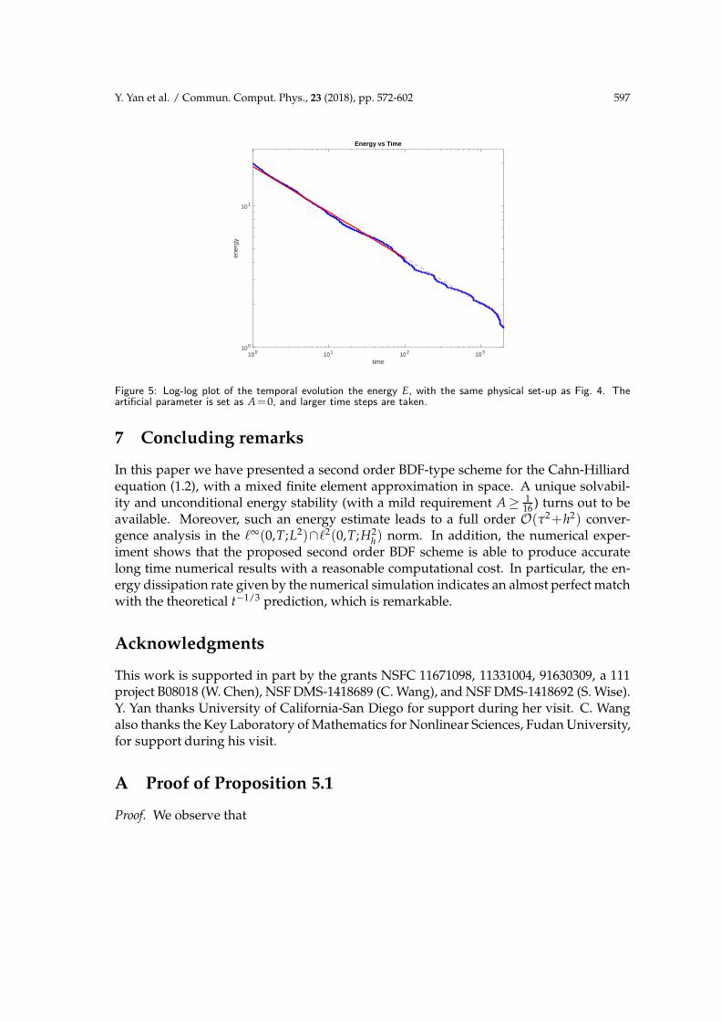
lar, Fig. 5 gives the energy dissipation curve for A= 0 with larger time steps chosen atdifferent coarsening process: τ = 0.04 on the time interval [0,100], τ = 0.08 on the timeinterval [100,2000]. In this log-log plot, the slope of the least square fit line is −0.3222,which indicates a nice consistency with the t−1/3 dissipation law.

These numerical simulation results have also provided many more insights on theproposed numerical scheme (2.2). Although a theoretical justification of the energy sta-bility is only available with A ≥ 1

16 , this numerical experiment has shown that such aconstraint may only be a theoretical issue. Indeed, the numerical energy stability is oftenobserved for any A≥0.

We make another observation that, although Figs. 4 and 5 give almost exactly thesame coarsening rate for the energy over time period [0,100], the numerical result dis-played in Fig. 4 seems to be more accurate, since the log-log oscillation over this timeperiod is weaker than the one displayed in Fig. 5. On the other hand, such a coarseningrate is only valid for short and medium time scales; after t=100 (for a surface diffusionε2=0.005), the t−1/3 coarsening rate may not be accurate any more, and the solutions areexpected to converge to a steady state. Over the time period [100, 1000], we believe thatthe numerical results in Fig. 4 are more accurate, due to the fact that the smaller time stepsizes have been used to create this figure.


100 101 102 103

time

100

101

ener

gy

Energy vs Time

Figure 5: Log-log plot of the temporal evolution the energy E, with the same physical set-up as Fig. 4. Theartificial parameter is set as A=0, and larger time steps are taken.

7 Concluding remarks

In this paper we have presented a second order BDF-type scheme for the Cahn-Hilliardequation (1.2), with a mixed finite element approximation in space. A unique solvabil-ity and unconditional energy stability (with a mild requirement A≥ 1

16 ) turns out to beavailable. Moreover, such an energy estimate leads to a full order O(τ2+h2) conver-gence analysis in the ℓ∞(0,T;L2)∩ℓ2(0,T;H2

h) norm. In addition, the numerical exper-iment shows that the proposed second order BDF scheme is able to produce accuratelong time numerical results with a reasonable computational cost. In particular, the en-ergy dissipation rate given by the numerical simulation indicates an almost perfect matchwith the theoretical t−1/3 prediction, which is remarkable.

Acknowledgments

This work is supported in part by the grants NSFC 11671098, 11331004, 91630309, a 111project B08018 (W. Chen), NSF DMS-1418689 (C. Wang), and NSF DMS-1418692 (S. Wise).Y. Yan thanks University of California-San Diego for support during her visit. C. Wangalso thanks the Key Laboratory of Mathematics for Nonlinear Sciences, Fudan University,for support during his visit.

A Proof of Proposition 5.1

Proof. We observe that


(un+1)3−(un+1h )3=(un+1)3−(Rhun+1)3+(Rhun+1)3−(un+1

h )3.

Therefore, we could separate the estimate of J2 into two parts:

‖(un+1)3−(Rhun+1)3‖2= ‖(

(un+1)2+un+1Rhun+1+(Rhun+1)2)

ρn+1‖2

≤ 8(‖un+1‖4∞+‖Rhun+1‖4

∞)‖ρn+1‖2

≤C11h2(q+1)‖un+1‖2Hq+1 , (A.1)

for some C11>0 that is independent of h and τ. The last estimate implies that

((un+1)3−(Rhun+1)3,−∆hσn+1h )≤

2C11h2(q+1)

ε2‖un+1‖2

Hq+1+ε2

8‖∆hσn+1

h ‖2.

Define u0 := 1|Ω| (u0,1). Observe that (Rhun−u0,1)=(un

h−u0,1)=0. In particular, (σnh ,1)=0,

for all n≥0. We assume, as is standard, that |u0|≤1. Now, for the second part, we applyHolder’s inequality and use the embedding H1(Ω) → L6(Ω), and we get

((Rhun+1)3−(un+1h )3,−∆hσn+1

h )≤‖(Rhun+1)3−(un+1h )3‖·‖∆hσn+1

h ‖

≤‖(Rhun+1)2+Rhun+1un+1h +(un+1

h )2‖L3 ·‖σn+1h ‖L6 ·‖∆hσn+1

h ‖

≤2(

‖Rhun+1‖2L6 +‖un+1

h ‖2L6

)

·‖σn+1h ‖L6 ·‖∆hσn+1

h ‖

≤4(

‖Rhun+1−u0‖2L6+‖un+1

h −u0‖2L6 +2|Ω|

13 |u0|

2)

·‖σn+1h ‖L6 ·‖∆hσn+1

h ‖

≤4C(

‖∇Rhun+1‖2+‖∇un+1h ‖2+2|Ω|

13

)

·‖∇σn+1h ‖·‖∆hσn+1

h ‖

≤4C(

‖∇un+1‖2+‖∇un+1h ‖2+2|Ω|

13

)

·‖∇σn+1h ‖·‖∆hσn+1

h ‖

≤4C(C+C1+1)·C‖∇σn+1h ‖·‖∆hσn+1

h ‖

≤C12‖σn+1h ‖

12 ·‖∆hσn+1

h ‖32 , (A.2)

for some C12>0 that is independent of τ and h. Next, we apply Young’s inequality,

ab≤ap

p+

bq

q,

with p=4 and q=4/3. By carefully balancing the coefficients, we obtain

((Rhun+1)3−(uh)3,−∆hσn+1

h )≤54

ε6C4

12‖σn+1h ‖2+

ε2

8‖∆hσn+1

h ‖2.

This in turn yields inequality (5.32). The proof of Proposition 5.1 is complete.


B Proof of Proposition 5.2

Proof. For n=0, inequality (5.30) indicates that

1

2‖σ1

h‖2+

τε2

2‖∆hσ1

h‖2≤

(

τ

2+

108τ

ε6C4

12

)

‖σ1h‖

2+2Ch2(q+1)∫ t1

0‖∂tu‖

2Hq+1 dt

+4Ch2(q+1)

ε2τ‖w1‖2

Hq+1+4

ε2C11τh2(q+1)‖u1‖2

Hq+1

+8C

ε2τh2(q+1)‖u0‖2

Hq+1+4

ε2Ch2(q+1)

∫ t1

0‖∂tu‖

2Hq+1dt

+4τ4C9+4τ4C10. (B.1)

Equivalently,

3

2‖σ1

h‖2+

τε2

2‖∆hσ1

h‖2≤ τ

(

3

2+

324

ε6C4

12

)

‖σ1h‖

2+6Ch2(q+1)∫ t1

0‖∂tu‖

2Hq+1 dt

+12Ch2(q+1)

ε2τ‖w1‖2

Hq+1+12

ε2C11τh2(q+1)‖u1‖2

Hq+1

+24C

ε2τh2(q+1)‖u0‖2

Hq+1+12

ε2Ch2(q+1)

∫ t1

0‖∂tu‖

2Hq+1dt

+12τ4C9+12τ4C10. (B.2)

Now, observe that∥

∥p1∥

∥

2

G= 3

2

∥

∥σ1h

∥

∥

2and

∥

∥pn+1∥

∥

2

G≥ 1

2

∥

∥

∥σn+1

h

∥

∥

∥. Summing (5.29) from k=2 to

k=n+1, adding (B.2), and keeping in mind (5.3) (the relationship between G-norm andL2-norm), we arrive at the following estimate for n≥1:

1

2‖σn+1

h ‖2+ε2τ

2

n

∑k=0

‖∆hσk+1h ‖2≤‖pn+1‖2

G+Aτ2‖∆hσn+1h ‖2+

ε2τ

2

n

∑k=0

‖∆hσk+1h ‖2

≤

(

1+108

ε6C4

12

)

τ‖σn+1h ‖2+

(

3

2+

324

ε6C4

12+40

ε2

)

τn−1

∑k=0

‖σk+1h ‖2+R,

where

R= h2(q+1)

(

9C+12

ε2

)

∫ T

0‖∂tu‖

2Hq+1 dt+h2(q+1) ·

12C

ǫ2τ

n

∑k=0

‖wk+1‖2Hq+1

+h2(q+1) 12C11+40C

ε2τ

n

∑k=0

‖uk+1‖2Hq+1+τ4 ·64

∫ T

0‖∂tttu‖

2dt

+τ4 ·8

ε2

(

32∫ T

0‖∂ttu‖

2dt+A2∫ T

0‖∂t∆u‖2dt

)

+12τ4C9+12τ4C10

≤ C13(ε)(h2(q+1)+τ4).


Under the time step requirement (5.34), which implies that

1

4‖σn+1

h ‖2+ε2τ

4

n

∑k=0

‖∆hσk+1h ‖2≤

(

3

2+

324

ε6C4

12+40

ε2

)

τn

∑k=1

‖σkh‖

2

+ C13(ε)(h2(q+1)+τ4).

Now, we can apply the discrete Gronwall inequality (5.1) and get

‖σn+1h ‖2+ε2τ

n+1

∑k=1

‖∆hσkh‖

2≤C15(T,ε)(h2(q+1)+τ4).

This completes the proof of Proposition 5.2.

References

[1] S. M. Allen and J. W. Cahn. A microscopic theory for antiphase boundary motion and itsapplication to antiphase domain coarsening. Acta. Metall., 27:1085, 1979.

[2] A. Aristotelous, O. Karakasian, and S.M. Wise. Adaptive, second-order in time, primitive-variable discontinuous Galerkin schemes for a Cahn-Hilliard equation with a mass source.IMA J. Numer. Anal., 35:1167–1198, 2015.

[3] A. Baskaran, Z. Hu, J. Lowengrub, C. Wang, S.M. Wise, and P. Zhou. Energy stable andefficient finite-difference nonlinear multigrid schemes for the modified phase field crystalequation. J. Comput. Phys., 250:270–292, 2013.

[4] A. Baskaran, J. Lowengrub, C. Wang, and S. Wise. Convergence analysis of a second orderconvex splitting scheme for the modified phase field crystal equation. SIAM J. Numer. Anal.,51:2851–2873, 2013.

[5] B. Benesova, C. Melcher, and E. Suli. An implicit midpoint spectral approximation of non-local Cahn-Hilliard equations. SIAM J. Numer. Anal., 52:1466–1496, 2014.

[6] S. Brenner and L. Scott. The Mathematical Theory of Finite Element Methods. Springer-Verlag,3rd edition, 2010.

[7] J.W. Cahn and J.E. Hilliard. Free energy of a nonuniform system. i. interfacial free energy. J.Chem. Phys., 28:258–267, 1958.

[8] W. Chen, S. Conde, C. Wang, X. Wang, and S.M. Wise. A linear energy stable scheme for athin film model without slope selection. J. Sci. Comput., 52:546–562, 2012.

[9] W. Chen, Y. Liu, C. Wang, and S.M. Wise. An optimal-rate convergence analysis of a fully dis-crete finite difference scheme for Cahn-Hilliard-Hele-Shaw equation. Math. Comp., 85:2231–2257, 2016.

[10] W. Chen, C. Wang, X. Wang, and S.M. Wise. A linear iteration algorithm for energy stablesecond order scheme for a thin film model without slope selection. J. Sci. Comput., 59:574–601, 2014.

[11] K. Cheng, C. Wang, S.M. Wise, and X. Yue. A second-order, weakly energy-stable pseudo-spectral scheme for the Cahn-Hilliard equation and its solution by the homogeneous lineariteration method. J. Sci. Comput., 69:1083–1114, 2016.

[12] A. Christlieb, J. Jones, K. Promislow, B. Wetton, and M. Willoughby. High accuracy solutionsto energy gradient flows from material science models. J. Comput. Phys., 257:193–215, 2014.


[13] A. Diegel, X. Feng, and S.M. Wise. Convergence analysis of an unconditionally stablemethod for a Cahn-Hilliard-Stokes system of equations. SIAM J. Numer. Anal., 53:127–152,2015.

[14] A. Diegel, C. Wang, X. Wang, and S.M. Wise. Convergence analysis and error estimates fora second order accurate finite element method for the Cahn-Hilliard-Navier-Stokes system.Numer. Math., 2017. accepted and in press.

[15] A. Diegel, C. Wang, and S.M. Wise. Stability and convergence of a second order mixed finiteelement method for the Cahn-Hilliard equation. IMA J. Numer. Anal., 36:1867–1897, 2016.

[16] Q. Du and R. Nicolaides. Numerical analysis of a continuum model of a phase transition.SIAM J. Numer. Anal., 28:1310–1322, 1991.

[17] D. Eyre. Unconditionally gradient stable time marching the Cahn-Hilliard equation. InJ. W. Bullard, R. Kalia, M. Stoneham, and L.Q. Chen, editors, Computational and MathematicalModels of Microstructural Evolution, volume 53, pages 1686–1712, Warrendale, PA, USA, 1998.Materials Research Society.

[18] W. Feng, A.J. Salgado, C. Wang, and S.M. Wise. Preconditioned steepest descent methods forsome nonlinear elliptic equations involving p-Laplacian terms. J. Comput. Phys., 334:45–67,2017.

[19] X. Feng and A. Prohl. Error analysis of a mixed finite element method for the Cahn-Hilliardequation. Numer. Math., 99:47–84, 2004.

[20] X. Feng and S.M. Wise. Analysis of a fully discrete finite element approximation of aDarcy-Cahn-Hilliard diffuse interface model for the Hele-Shaw flow. SIAM J. Numer. Anal.,50:1320–1343, 2012.

[21] D. Furihata. A stable and conservative finite difference scheme for the Cahn-Hilliard equa-tion. Numer. Math., 87:675–699, 2001.

[22] Z. Guan, J.S. Lowengrub, C. Wang, and S.M. Wise. Second-order convex splitting schemesfor nonlocal Cahn-Hilliard and Allen-Cahn equations. J. Comput. Phys., 277:48–71, 2014.

[23] Z. Guan, C. Wang, and S.M. Wise. A convergent convex splitting scheme for the periodicnonlocal Cahn-Hilliard equation. Numer. Math., 128:377–406, 2014.

[24] F. Guillen-Gonzalez and G. Tierra. Second order schemes and time-step adaptivity for Allen-Cahn and Cahn-Hilliard models. Comput. Math. Appl., 68(8):821–846, 2014.

[25] J. Guo, C. Wang, S.M. Wise, and X. Yue. An H2 convergence of a second-order convex-splitting, finite difference scheme for the three-dimensional Cahn-Hilliard equation. Commu.Math. Sci., 14:489–515, 2016.

[26] D. Han, A. Brylev, X. Yang, and Z. Tan. Numerical analysis of second order, fully discreteenergy stable schemes for phase field models of two phase incompressible flows. J. Sci.Comput., 70:965–989, 2017.

[27] D. Han and X. Wang. A second order in time, uniquely solvable, unconditionally stablenumerical scheme for Cahn-Hilliard-Navier-Stokes equation. J. Comput. Phys., 290:139–156,2015.

[28] Z. Hu, S. Wise, C. Wang, and J. Lowengrub. Stable and efficient finite-difference nonlinear-multigrid schemes for the phase-field crystal equation. J. Comput. Phys., 228:5323–5339, 2009.

[29] L. Ju, X. Li, Z. Qiao, and H. Zhang. Energy stability and convergence of exponential timedifferencing schemes for the epitaxial growth model without slope selection. Math. Comp.,2017. Accepted and in press.

[30] D. Li and Z. Qiao. On second order semi-implicit Fourier spectral methods for 2D Cahn-Hilliard equations. J. Sci. Comput., 70:301–341, 2017.

[31] D. Li, Z. Qiao, and T. Tang. Characterizing the stabilization size for semi-implicit Fourier-


spectral method to phase field equations. SIAM J. Numer. Anal., 54:1653–1681, 2016.[32] J. Shen, C. Wang, X. Wang, and S.M. Wise. Second-order convex splitting schemes for gra-

dient flows with Ehrlich-Schwoebel type energy: Application to thin film epitaxy. SIAM J.Numer. Anal., 50:105–125, 2012.

[33] J. Shen, X. Yang, and H. Yu. Efficient energy stable numerical schemes for a phase fieldmoving contact line model. J. Comput. Phys., 284:617–630, 2015.

[34] C. Wang, X. Wang, and S.M. Wise. Unconditionally stable schemes for equations of thin filmepitaxy. Discrete Contin. Dyn. Sys. A, 28:405–423, 2010.

[35] C. Wang and S.M. Wise. An energy stable and convergent finite-difference scheme for themodified phase field crystal equation. SIAM J. Numer. Anal., 49:945–969, 2011.

[36] S.M. Wise. Unconditionally stable finite difference, nonlinear multigrid simulation of theCahn-Hilliard-Hele-Shaw system of equations. J. Sci. Comput., 44:38–68, 2010.

[37] S.M. Wise, C. Wang, and J.S. Lowengrub. An energy stable and convergent finite-differencescheme for the phase field crystal equation. SIAM J. Numer. Anal., 47:2269–2288, 2009.

[38] X. Wu, G.J. van Zwieten, and K.G. van der Zee. Stabilized second-order convex splittingschemes for Cahn-Hilliard models with application to diffuse-interface tumor-growth mod-els. Inter. J. Numer. Methods Biomed. Eng., 30:180–203, 2014.

[39] X. Yang. Linear, and unconditionally energy stable numerical schemes for the phase fieldmodel of homopolymer blends. J. Comput. Phys., 302:509–523, 2016.

[40] X. Yang and D. Han. Linearly first- and second-order, unconditionally energy stable schemesfor the phase field crystal model. J. Comput. Phys., 330:1116–1134, 2017.

[41] J. Zhao, Q. Wang, and X. Yang. Numerical approximations for a phase field dendritic crystalgrowth model based on the invariant energy quadratization approach. Inter. J. Num. Meth.Engr., 110:279–300, 2017.

ASecond-OrderEnergyStableBDFNumericalScheme for the …

Documents

Transcript of ASecond-OrderEnergyStableBDFNumericalScheme for the …