April 2015 Revenue Forecast Methodology and Technical ... · Tax and Revenue Division at...

STATE OF INDIANA Michael R. Pence

Governor

STATE BUDGET AGENCY 212 State House

Indianapolis, Indiana 46204-2796

317-232-5610

Brian E. Bailey

Director

April 2015 Revenue Forecast

Methodology and Technical Documentation

Table of Contents

Section I: Commentary on the Economic Forecast Section II: Economic Indicators for Indiana

Section III: Models Used in the Forecast Section IV: Technical Explanations

2

Introduction This document provides an overview to the April 2015 state revenue forecast. Historically, this document has included step-by-step calculations to achieve the total forecast. This practice has been discontinued due to proprietary data used from the committee’s economic forecaster. Instead of the calculation instructions, each model’s specifications, summary statistics, and forecasts are included. For further information and assistance in the calculation of models, please contact the State Budget Agency’s Tax and Revenue Division at 317-232-5610. Revenue Forecast Committee The revenue forecast committee is comprised of members from both the executive and legislative branches. Staff from both the State Budget Agency and Legislative Services Agency have a vital role in the process by assisting with data analysis and modeling. Each forecast model and revenue estimate is agreed to by the technical committee on a consensus basis. Technical Committee: Eric Bussis, State Budget Agency David Dukes, House Republican Appointee Erik Gonzalez, House Democratic Appointee Dr. John Mikesell, Indiana University SPEA Susan Preble, Senate Democratic Appointee David Reynolds, Senate Republican Appointee Budget Committee Appointed Advisors: John Grew William Sheldrake

Key Contributors: Vanessa DeVeau Bachle, State Budget Agency Heath Holloway, Legislative Services Agency Matthew Hutchinson, State Budget Agency Randhir Jha, Legislative Services Agency Dr. Jim Landers, Legislative Services Agency Megan McDermott, State Budget Agency

Economic Forecast The forecast committee uses economic forecasts from IHS Global Insight, Inc. Forecasts cited in this document are provided by IHS, a leading economic consulting firm. IHS is routinely ranked among the leading economic forecasters in studies by The Wall Street Journal and Bloomberg Markets. The State Budget Agency is also provided with access to the Indiana forecasts of Indiana University’s Center for Econometric Model Research (“CEMR”). The committee reviews the projections for comparison.

3

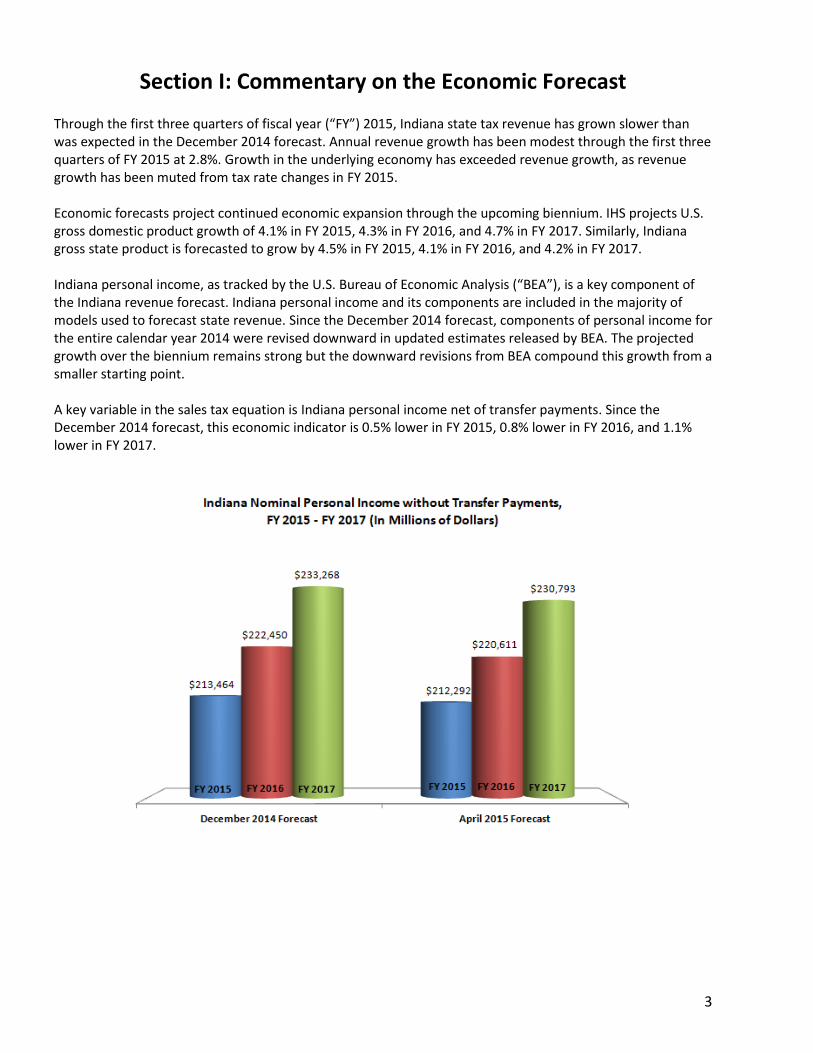
Section I: Commentary on the Economic Forecast Through the first three quarters of fiscal year (“FY”) 2015, Indiana state tax revenue has grown slower than was expected in the December 2014 forecast. Annual revenue growth has been modest through the first three quarters of FY 2015 at 2.8%. Growth in the underlying economy has exceeded revenue growth, as revenue growth has been muted from tax rate changes in FY 2015. Economic forecasts project continued economic expansion through the upcoming biennium. IHS projects U.S. gross domestic product growth of 4.1% in FY 2015, 4.3% in FY 2016, and 4.7% in FY 2017. Similarly, Indiana gross state product is forecasted to grow by 4.5% in FY 2015, 4.1% in FY 2016, and 4.2% in FY 2017. Indiana personal income, as tracked by the U.S. Bureau of Economic Analysis (“BEA”), is a key component of the Indiana revenue forecast. Indiana personal income and its components are included in the majority of models used to forecast state revenue. Since the December 2014 forecast, components of personal income for the entire calendar year 2014 were revised downward in updated estimates released by BEA. The projected growth over the biennium remains strong but the downward revisions from BEA compound this growth from a smaller starting point. A key variable in the sales tax equation is Indiana personal income net of transfer payments. Since the December 2014 forecast, this economic indicator is 0.5% lower in FY 2015, 0.8% lower in FY 2016, and 1.1% lower in FY 2017.

4

The BEA’s downward revision also impacted Indiana wage and salary disbursements. This economic indicator is the main determinant of the individual income tax forecast. Since the December 2014 forecast, Indiana wage and salary disbursements have decreased approximately one billion dollars (0.7%) for each fiscal year of the forecast period.

The corporate income tax model utilized by the committee is driven by BEA U.S. corporate profits. These profits, which increased by 1.2% in FY 2014, are forecasted by IHS Global Insight to increase by 4.4% in FY 2015, 8.1% in FY 2016, and 2.3% in FY 2017. Although still strong, growth in corporate profits at the time of the December forecast for FY 2015 was 8.9%, which is half of the forecasted growth rate The committee continues to monitor both the size and shifts in the labor market. Over the past year, the number of employed Hoosiers has increased and the unemployment rate has decreased. In the forecast period, the unemployment rate is projected to decline and reach 5.5% in the beginning of calendar year 2016. The labor force participation rate and the changing demographics of the labor force are key aspects to Indiana’s economic outlook. At the time of the December 2014 forecast, IHS Global Insight forecasted an Indiana labor force participation rate of 61.0% in FY 2015. In the latest forecast this is projected to reach 61.4% in FY 2015, 61.6% in FY 2016, and 61.6% in FY 2017. The number of Indiana residents employed as a percent of population has also recovered in the last year. While the rate remained above 60% from 1988 to 2008, it fell to 55% in 2010. The rate is forecasted to remain around 58% throughout the upcoming biennium.

5

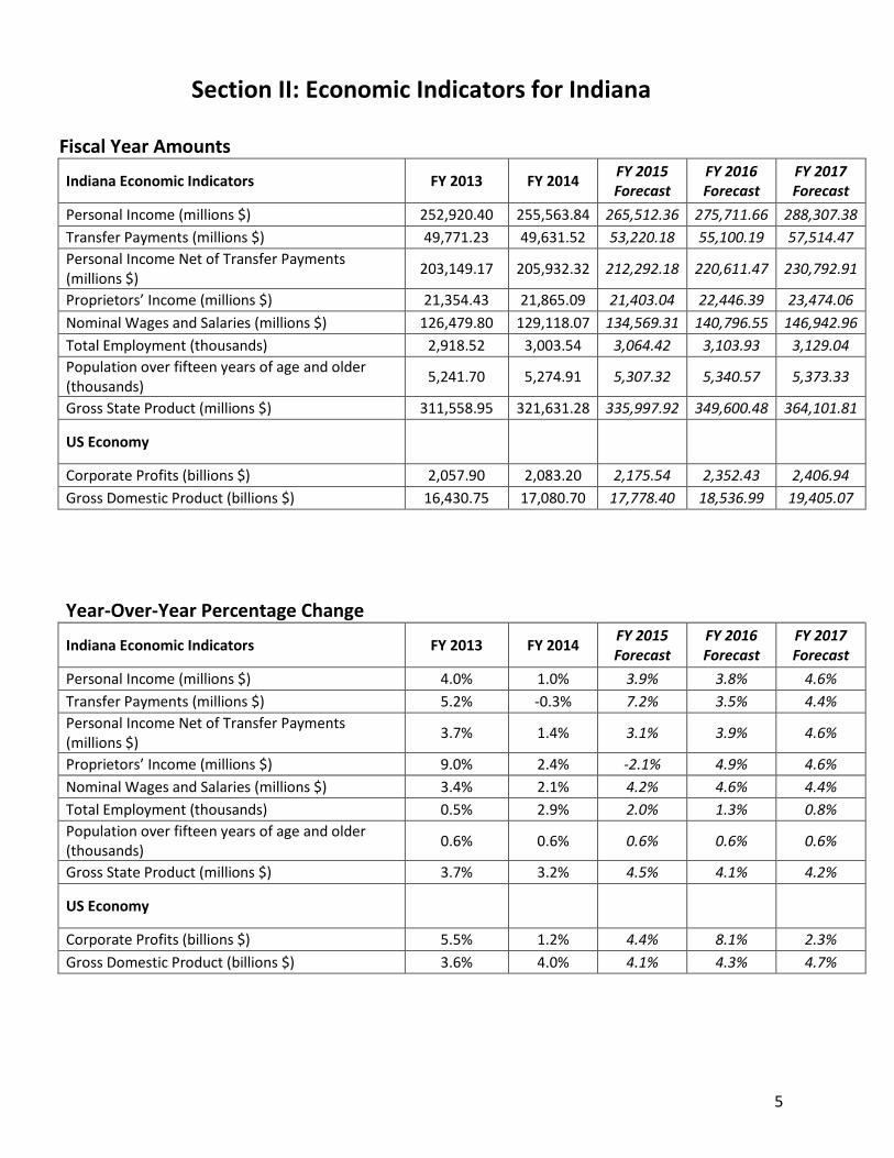
Section II: Economic Indicators for Indiana Fiscal Year Amounts

Indiana Economic Indicators FY 2013 FY 2014 FY 2015 Forecast

FY 2016 Forecast

FY 2017 Forecast

Personal Income (millions $) 252,920.40 255,563.84 265,512.36 275,711.66 288,307.38

Transfer Payments (millions $) 49,771.23 49,631.52 53,220.18 55,100.19 57,514.47

Personal Income Net of Transfer Payments (millions $)

203,149.17 205,932.32 212,292.18 220,611.47 230,792.91

Proprietors’ Income (millions $) 21,354.43 21,865.09 21,403.04 22,446.39 23,474.06

Nominal Wages and Salaries (millions $) 126,479.80 129,118.07 134,569.31 140,796.55 146,942.96

Total Employment (thousands) 2,918.52 3,003.54 3,064.42 3,103.93 3,129.04

Population over fifteen years of age and older (thousands)

5,241.70 5,274.91 5,307.32 5,340.57 5,373.33

Gross State Product (millions $) 311,558.95 321,631.28 335,997.92 349,600.48 364,101.81

US Economy

Corporate Profits (billions $) 2,057.90 2,083.20 2,175.54 2,352.43 2,406.94

Gross Domestic Product (billions $) 16,430.75 17,080.70 17,778.40 18,536.99 19,405.07

Year-Over-Year Percentage Change

Indiana Economic Indicators FY 2013 FY 2014 FY 2015 Forecast

FY 2016 Forecast

FY 2017 Forecast

Personal Income (millions $) 4.0% 1.0% 3.9% 3.8% 4.6%

Transfer Payments (millions $) 5.2% -0.3% 7.2% 3.5% 4.4%

Personal Income Net of Transfer Payments (millions $)

3.7% 1.4% 3.1% 3.9% 4.6%

Proprietors’ Income (millions $) 9.0% 2.4% -2.1% 4.9% 4.6%

Nominal Wages and Salaries (millions $) 3.4% 2.1% 4.2% 4.6% 4.4%

Total Employment (thousands) 0.5% 2.9% 2.0% 1.3% 0.8%

Population over fifteen years of age and older (thousands)

0.6% 0.6% 0.6% 0.6% 0.6%

Gross State Product (millions $) 3.7% 3.2% 4.5% 4.1% 4.2%

US Economy

Corporate Profits (billions $) 5.5% 1.2% 4.4% 8.1% 2.3%

Gross Domestic Product (billions $) 3.6% 4.0% 4.1% 4.3% 4.7%

6

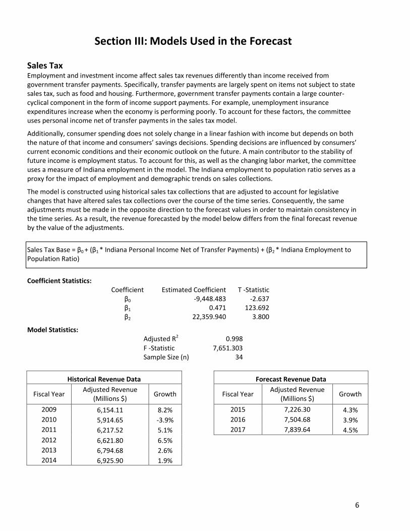
Section III: Models Used in the Forecast Sales Tax Employment and investment income affect sales tax revenues differently than income received from government transfer payments. Specifically, transfer payments are largely spent on items not subject to state sales tax, such as food and housing. Furthermore, government transfer payments contain a large counter-cyclical component in the form of income support payments. For example, unemployment insurance expenditures increase when the economy is performing poorly. To account for these factors, the committee uses personal income net of transfer payments in the sales tax model.

Additionally, consumer spending does not solely change in a linear fashion with income but depends on both the nature of that income and consumers’ savings decisions. Spending decisions are influenced by consumers’ current economic conditions and their economic outlook on the future. A main contributor to the stability of future income is employment status. To account for this, as well as the changing labor market, the committee uses a measure of Indiana employment in the model. The Indiana employment to population ratio serves as a proxy for the impact of employment and demographic trends on sales collections.

The model is constructed using historical sales tax collections that are adjusted to account for legislative changes that have altered sales tax collections over the course of the time series. Consequently, the same adjustments must be made in the opposite direction to the forecast values in order to maintain consistency in the time series. As a result, the revenue forecasted by the model below differs from the final forecast revenue by the value of the adjustments.

Sales Tax Base = β0 + (β1 * Indiana Personal Income Net of Transfer Payments) + (β2 * Indiana Employment to Population Ratio)

Coefficient Statistics: Coefficient Estimated Coefficient T -Statistic

β0 -9,448.483 -2.637 β1 0.471 123.692 β2 22,359.940 3.800

Model Statistics: Adjusted R2 0.998

F -Statistic 7,651.303 Sample Size (n) 34

Historical Revenue Data

Forecast Revenue Data

Fiscal Year Adjusted Revenue

(Millions $) Growth


(Millions $) Growth

2009 6,154.11 8.2%

2015 7,226.30 4.3%

2010 5,914.65 -3.9%

2016 7,504.68 3.9%

2011 6,217.52 5.1%

2017 7,839.64 4.5%

2012 6,621.80 6.5%

2013 6,794.68 2.6%

2014 6,925.90 1.9%

7

Individual Income Tax The Committee determined that the income tax forecast should be derived using three separate equations to account for differences between income taxes collected through estimated payments, tax withheld from salary and wage disbursements, and income tax return filings. The selected equations use quarterly data rather than fiscal year data to account for fluctuations throughout each fiscal year. Estimated payments are mainly collected on investment income, sole proprietors’ income, and business income. BEA’s Indiana proprietors’ income comprises the majority of these income components. The estimated payments equation used by the committee includes Indiana proprietors’ income, the previous year’s quarterly estimated payments, and a set of binary variables to account for seasonal factors and structural changes in estimated payment activity. Withholding on income tax is driven mainly by Indiana salary and wage disbursements. Additionally, income tax can be withheld on pension benefits, retirement benefits, and some government transfer payments. The final settlement amounts include refunds for overpayment and all forms of final remits. The committee used a five year historical average to estimate a fiscal year total. As with sales, both the withholding and the final settlements series have been adjusted to maintain a consistent time series despite legislative changes. The final settlements series includes adjustments for both the College Choice 529 Credit and the Earned Income Tax Credit. Additionally, over the period of the forecast, the income tax rate is scheduled to be reduced from 3.4% in the middle of FY 2015 to 3.23% by the middle of FY 2017. As a result, while many of the explanatory models used to forecast income tax collections are expected to increase, total collections will increase more slowly.

Total Income Tax Forecast = Estimated Payments + Withholding + Settlements

8

Income Tax: Estimated Payments Estimated Payments Tax Base = β0 + (β1 * Indiana Proprietor’s Income) + (β2 * Dummy CY Q1) + (β3 * Dummy CY Q2) + (β4 * Dummy CY Q3) + (β5 * Year Lag of Estimated Payments) + (β6 * Dummy for CY 2008 Q2) + (β7 * Dummy FY 2009 and After) Coefficient Statistics:

Coefficient Estimated Coefficient T -Statistic β0 -174.296 -0.337 β1 0.079 2.314 β2 1,984.802 5.859 β3 2,967.581 6.847 β4 1,716.789 5.742 β5 0.335 3.969 β6 2,780.507 3.899 β7 -1,037.438 -4.513

Model Statistics:

Adjusted R2 0.89 F -Statistic 80.545 Sample Size (n) 70

Historical Data

Forecast Data


(Millions $) Growth


(Millions $) Growth

2009 471.72 -33.0%

2015 461.77 7.1%

2010 356.10 -24.5%

2016 446.11 -3.4%

2011 378.85 6.4%

2017 450.23 0.9%

2012 394.36 4.1%

2013 433.36 9.9%

2014 431.24 -0.5%

9

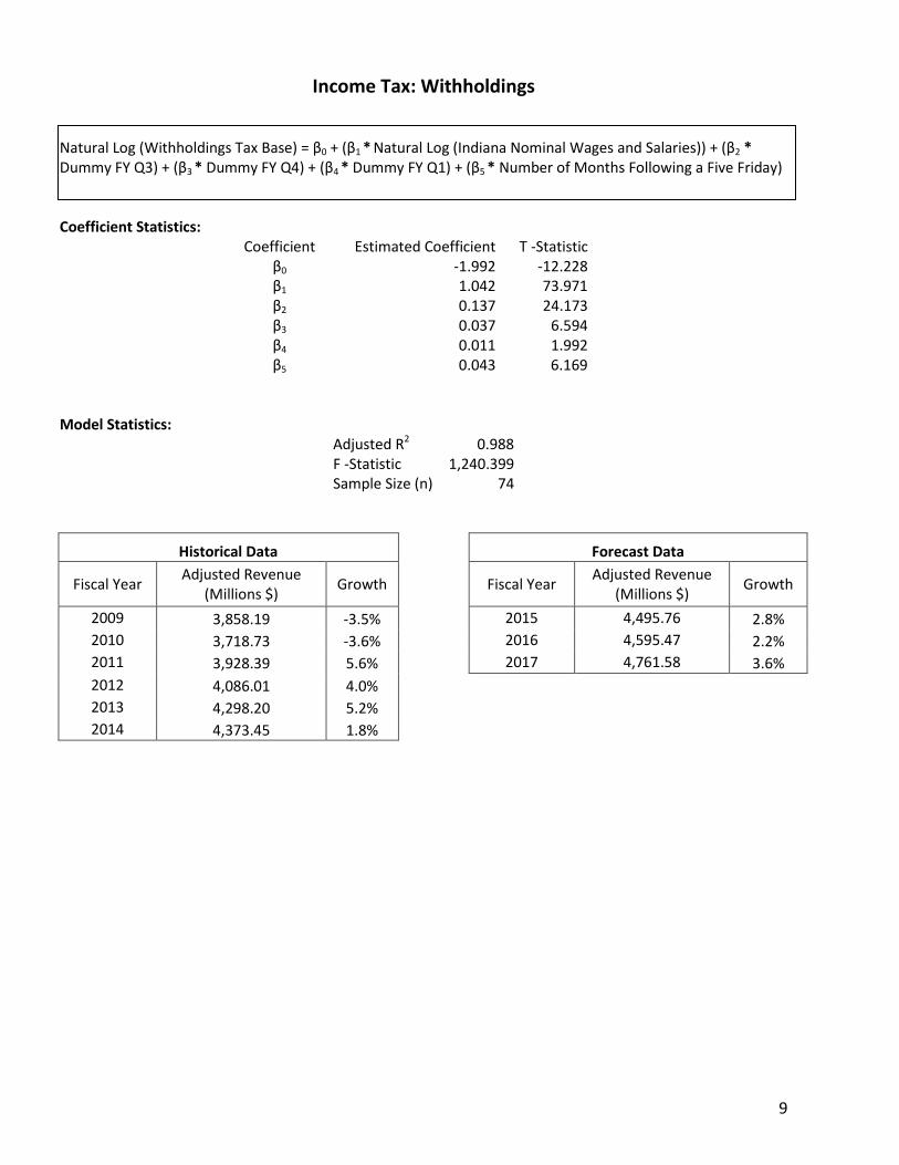
Income Tax: Withholdings

Natural Log (Withholdings Tax Base) = β0 + (β1 * Natural Log (Indiana Nominal Wages and Salaries)) + (β2 * Dummy FY Q3) + (β3 * Dummy FY Q4) + (β4 * Dummy FY Q1) + (β5 * Number of Months Following a Five Friday) Coefficient Statistics:

Coefficient Estimated Coefficient T -Statistic β0 -1.992 -12.228 β1 1.042 73.971 β2 0.137 24.173 β3 0.037 6.594 β4 0.011 1.992 β5 0.043 6.169

Model Statistics:

Adjusted R2 0.988 F -Statistic 1,240.399 Sample Size (n) 74

Historical Data

Forecast Data


(Millions $) Growth


(Millions $) Growth

2009 3,858.19 -3.5%

2015 4,495.76 2.8%

2010 3,718.73 -3.6%

2016 4,595.47 2.2%

2011 3,928.39 5.6%

2017 4,761.58 3.6%

2012 4,086.01 4.0%

2013 4,298.20 5.2%

2014 4,373.45 1.8%

10

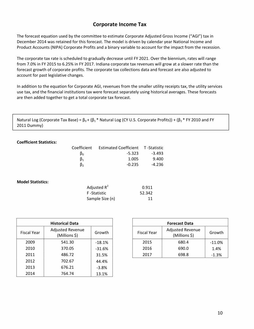
Corporate Income Tax The forecast equation used by the committee to estimate Corporate Adjusted Gross Income (“AGI”) tax in December 2014 was retained for this forecast. The model is driven by calendar year National Income and Product Accounts (NIPA) Corporate Profits and a binary variable to account for the impact from the recession. The corporate tax rate is scheduled to gradually decrease until FY 2021. Over the biennium, rates will range from 7.0% in FY 2015 to 6.25% in FY 2017. Indiana corporate tax revenues will grow at a slower rate than the forecast growth of corporate profits. The corporate tax collections data and forecast are also adjusted to account for past legislative changes. In addition to the equation for Corporate AGI, revenues from the smaller utility receipts tax, the utility services use tax, and the financial institutions tax were forecast separately using historical averages. These forecasts are then added together to get a total corporate tax forecast. Natural Log (Corporate Tax Base) = β0 + (β1 * Natural Log (CY U.S. Corporate Profits)) + (β2 * FY 2010 and FY 2011 Dummy) Coefficient Statistics:

Coefficient Estimated Coefficient T -Statistic β0 -5.323 -3.493 β1 1.005 9.400 β2 -0.235 -4.236

Model Statistics:


Historical Data

Forecast Data


(Millions $) Growth


(Millions $) Growth

2009 541.30 -18.1%

2015 680.4 -11.0%

2010 370.05 -31.6%

2016 690.0 1.4%

2011 486.72 31.5%

2017 698.8 -1.3%

2012 702.67 44.4%

2013 676.21 -3.8%

2014 764.74 13.1%

11

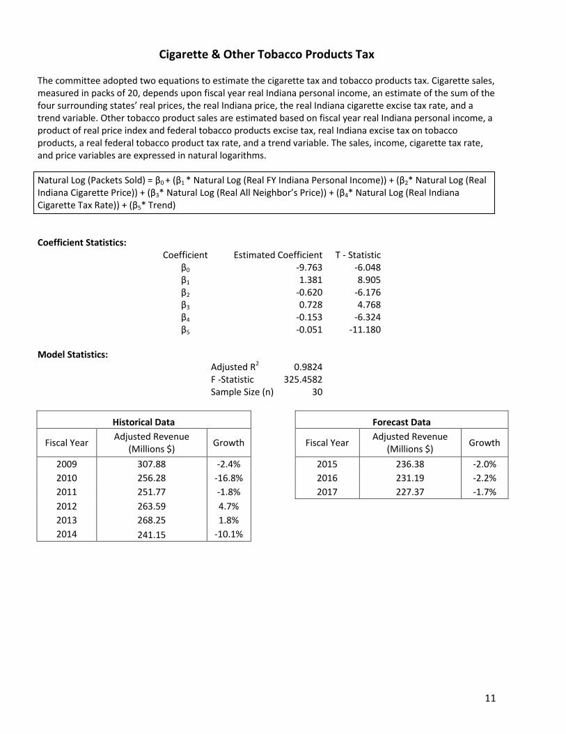
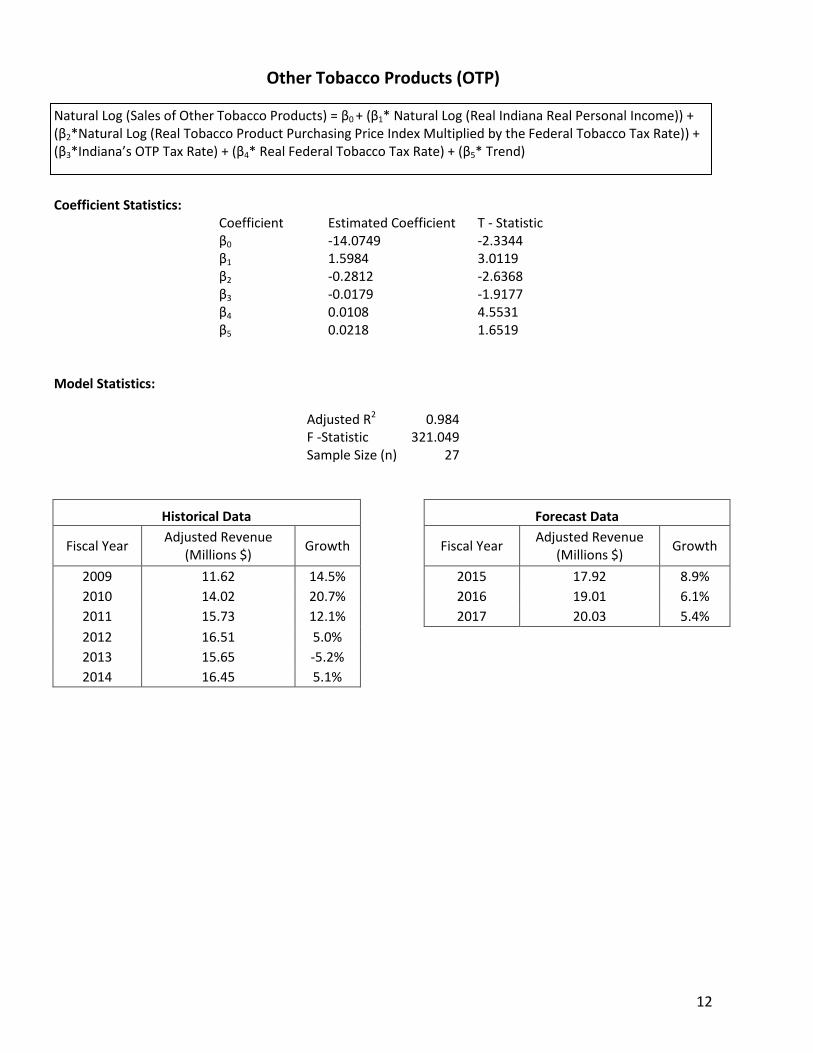
Cigarette & Other Tobacco Products Tax The committee adopted two equations to estimate the cigarette tax and tobacco products tax. Cigarette sales, measured in packs of 20, depends upon fiscal year real Indiana personal income, an estimate of the sum of the four surrounding states’ real prices, the real Indiana price, the real Indiana cigarette excise tax rate, and a trend variable. Other tobacco product sales are estimated based on fiscal year real Indiana personal income, a product of real price index and federal tobacco products excise tax, real Indiana excise tax on tobacco products, a real federal tobacco product tax rate, and a trend variable. The sales, income, cigarette tax rate, and price variables are expressed in natural logarithms. Natural Log (Packets Sold) = β0 + (β1 * Natural Log (Real FY Indiana Personal Income)) + (β2* Natural Log (Real Indiana Cigarette Price)) + (β3* Natural Log (Real All Neighbor’s Price)) + (β4* Natural Log (Real Indiana Cigarette Tax Rate)) + (β5* Trend) Coefficient Statistics:

Coefficient Estimated Coefficient T - Statistic β0 -9.763 -6.048 β1 1.381 8.905 β2 -0.620 -6.176 β3 0.728 4.768 β4 -0.153 -6.324 β5 -0.051 -11.180

Model Statistics:


Historical Data

Forecast Data


(Millions $) Growth


(Millions $) Growth

2009 307.88 -2.4%

2015 236.38 -2.0%

2010 256.28 -16.8%

2016 231.19 -2.2%

2011 251.77 -1.8%

2017 227.37 -1.7%

2012 263.59 4.7%

2013 268.25 1.8%

2014 241.15 -10.1%

12

Other Tobacco Products (OTP) Natural Log (Sales of Other Tobacco Products) = β0 + (β1* Natural Log (Real Indiana Real Personal Income)) + (β2*Natural Log (Real Tobacco Product Purchasing Price Index Multiplied by the Federal Tobacco Tax Rate)) + (β3*Indiana’s OTP Tax Rate) + (β4* Real Federal Tobacco Tax Rate) + (β5* Trend) Coefficient Statistics:

Coefficient Estimated Coefficient T - Statistic β0 -14.0749 -2.3344 β1 1.5984 3.0119 β2 -0.2812 -2.6368 β3 -0.0179 -1.9177 β4 0.0108 4.5531 β5 0.0218 1.6519

Model Statistics:


Historical Data

Forecast Data


(Millions $) Growth


(Millions $) Growth

2009 11.62 14.5%

2015 17.92 8.9%

2010 14.02 20.7%

2016 19.01 6.1%

2011 15.73 12.1%

2017 20.03 5.4%

2012 16.51 5.0%

2013 15.65 -5.2%

2014 16.45 5.1%

13

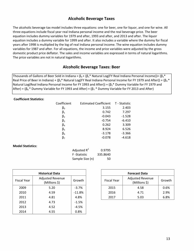
Alcoholic Beverage Taxes The alcoholic beverage tax model includes three equations: one for beer, one for liquor, and one for wine. All three equations include fiscal year real Indiana personal income and the real beverage price. The beer equation includes dummy variables for 1979 and after, 1993 and after, and 2013 and after. The liquor equation includes a dummy variable for 1999 and after. It also includes a variable where the dummy for fiscal years after 1998 is multiplied by the log of real Indiana personal income. The wine equation includes dummy variables for 1987 and after. For all equations, the income and price variables were adjusted by the gross domestic product price deflator. The sales and income variables are expressed in terms of natural logarithms. The price variables are not in natural logarithms.

Alcoholic Beverage Taxes: Beer

Thousands of Gallons of Beer Sold in Indiana = β0 + (β1* Natural Log(FY Real Indiana Personal Income))+ (β2* Real Price of Beer in Indiana) + (β3* Natural Log(FY Real Indiana Personal Income for FY 1979 and After)) + (β4 * Natural Log(Real Indiana Personal Income for FY 1993 and After)) + (β5* Dummy Variable for FY 1979 and After) + (β6 * Dummy Variable for FY 1993 and After) + (β7 * Dummy Variable for FY 2013 and After)

Coefficient Statistics:

Coefficient Estimated Coefficient T - Statistic β0 3.155 2.403 β1 0.742 7.297 β2 -0.043 -1.528 β3 -0.754 -6.410 β4 0.262 3.309 β5 8.924 6.526 β6 -3.178 -3.366 β7 -0.078 -4.618

Model Statistics:


Historical Data

Forecast Data


(Millions $) Growth


(Millions $) Growth

2009 5.20 -3.7%

2015 4.58 0.6%

2010 4.59 -11.8%

2016 4.71 2.9%

2011 4.81 4.8%

2017 5.03 6.8%

2012 4.73 -1.5%

2013 4.52 -4.5%

2014 4.55 0.8%

14

Alcoholic Beverage Taxes: Liquor Thousands of Gallons of Liquor Sold in Indiana = β0 + (β1 * Natural Log (Real Indiana Personal Income)) + (β2 * Real Price of Liquor in Indiana) + (β3 * Natural Log (FY Real Indiana Personal Income for FY 1999 and After)) + (β4 * Dummy Variable for FY 1999 and After) Coefficient Statistics:

Coefficient Estimated Coefficient T - Statistic β0 16.706 19.461 β1 -0.593 -8.657 β2 -0.072 -14.656 β3 2.479 9.626 β4 -30.079 -9.513

Model Statistics:


Historical Data

Forecast Data


(Millions $) Growth


(Millions $) Growth

2009 8.91 -1.1%

2015 10.41 0.6%

2010 6.26 -29.8%

2016 10.71 2.9%

2011 9.12 45.7%

2017 11.44 6.8%

2012 9.44 3.6%

2013 10.26 8.7%

2014 10.35 0.8%

15

Alcoholic Beverage Taxes: Wine Thousands of Gallons of Wine Sold in Indiana = β0 + (β1* Natural Log (Real Indiana Personal Income)) + (β2 * Real Price of Wine in Indiana) + (β3 * Dummy Variable for 1987 and After) Coefficient Statistics:

Coefficient Estimated Coefficient T - Statistic β0 1.330 0.571 β1 0.842 4.965 β2 -0.533 -5.214 β3 -0.269 -2.812

Statistics:


Historical Data

Forecast Data


(Millions $) Growth


(Millions $) Growth

2009 1.99 -0.2%

2015 2.21 0.6%

2010 1.86 -6.6%

2016 2.28 2.9%

2011 2.18 17.3%

2017 2.43 6.8%

2012 2.22 2.0%

2013 2.22 -0.3%

2014 2.20 -0.8%

16

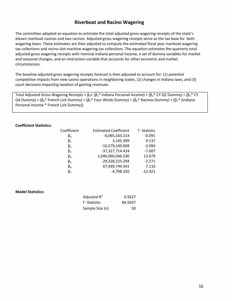
Riverboat and Racino Wagering The committee adopted an equation to estimate the total adjusted gross wagering receipts of the state’s eleven riverboat casinos and two racinos. Adjusted gross wagering receipts serve as the tax base for both wagering taxes. These estimates are then adjusted to compute the estimated fiscal year riverboat wagering tax collections and racino slot machine wagering tax collections. The equation estimates the quarterly total adjusted gross wagering receipts with nominal Indiana personal income, a set of dummy variables for market and seasonal changes, and an interaction variable that accounts for other economic and market circumstances. The baseline adjusted gross wagering receipts forecast is then adjusted to account for: (1) potential competitive impacts from new casino operations in neighboring states, (2) changes in Indiana laws, and (3) court decisions impacting taxation of gaming revenues. Total Adjusted Gross Wagering Receipts = β0+ (β1* Indiana Personal Income) + (β2* CY Q2 Dummy) + (β3* CY Q4 Dummy) + (β4* French Lick Dummy) + (β5* Four Winds Dummy) + (β6* Racinos Dummy) + (β7* (Indiana Personal Income * French Lick Dummy)) Coefficient Statistics:

Coefficient Estimated Coefficient T -Statistic β0 -6,065,163.214 -0.091 β1 3,145.399 9.137 β2 -10,579,149.009 -2.094 β3 -37,327,714.424 -7.607 β4 1,046,060,046.536 13.679 β5 -29,328,225.294 -2.271 β6 67,939,744.341 7.110 β7 -4,798.350 -12.421

Model Statistics:

Adjusted R2 0.9227

F -Statistic 84.5937

Sample Size (n) 50

17

Riverboat and Racino Wagering

Riverboat Wagering Historical Data

Riverboat Wagering Forecast Data


(Millions $) Growth


(Millions $) Growth

2009 545.40 -6.4%

2015 334.24 -8.0%

2010 538.10 -1.3%

2016 320.47 -4.1%

2011 529.05 -1.7%

2017 319.02 -0.5%

2012 496.55 -6.1%

2013 448.65 -9.6%

2014 363.32 -19.0%

Racino Wagering Historical Data

Racino Wagering Forecast Data


(Millions $) Growth


(Millions $) Growth

2009 107.70

2015 112.17 1.3%

2010 120.80 12.2%

2016 109.57 -2.3%

2011 131.30 8.7%

2017 108.49 -1.0%

2012 117.60 -10.4%

2013 105.90 -9.9%

2014 110.70 4.5%

18

Section IV: Technical Explanations

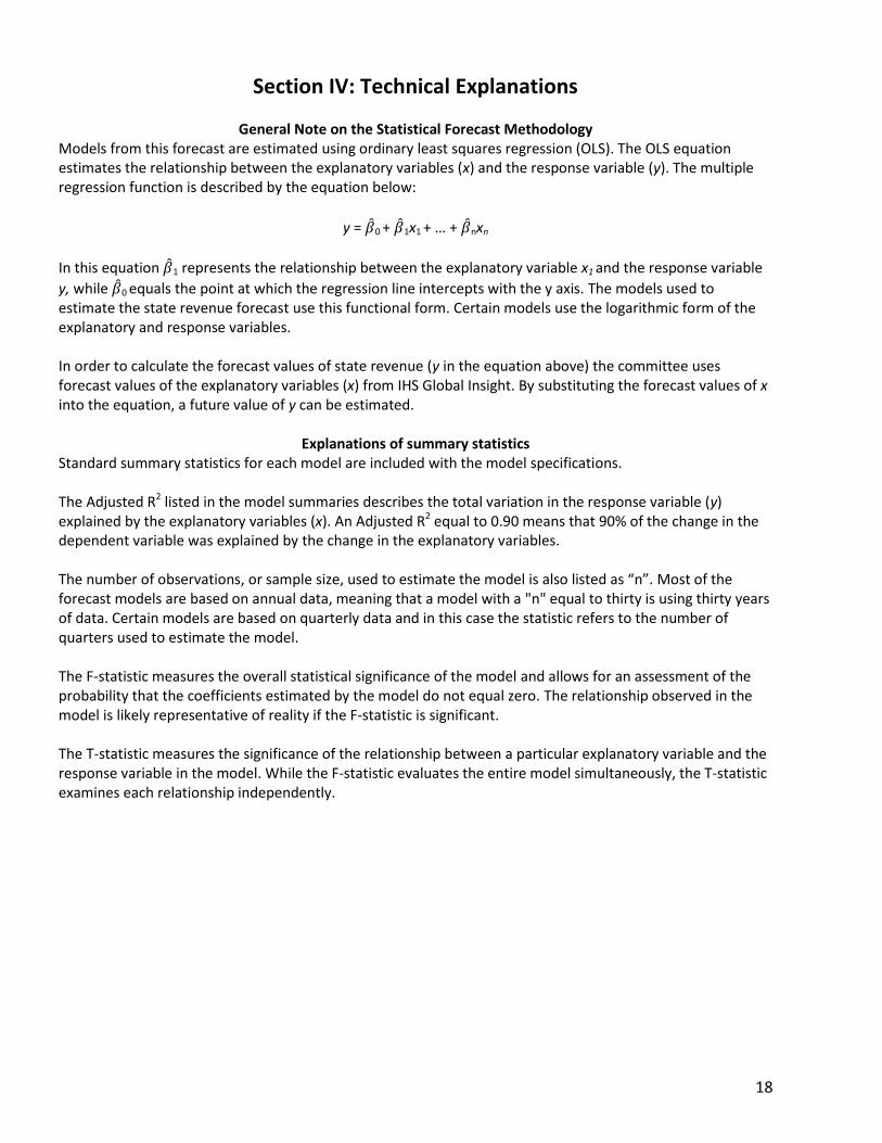
General Note on the Statistical Forecast Methodology Models from this forecast are estimated using ordinary least squares regression (OLS). The OLS equation estimates the relationship between the explanatory variables (x) and the response variable (y). The multiple regression function is described by the equation below:

y = 0 + 1x1 + … + nxn

In this equation 1 represents the relationship between the explanatory variable x1 and the response variable

y, while 0 equals the point at which the regression line intercepts with the y axis. The models used to estimate the state revenue forecast use this functional form. Certain models use the logarithmic form of the explanatory and response variables. In order to calculate the forecast values of state revenue (y in the equation above) the committee uses forecast values of the explanatory variables (x) from IHS Global Insight. By substituting the forecast values of x into the equation, a future value of y can be estimated.

Explanations of summary statistics Standard summary statistics for each model are included with the model specifications. The Adjusted R2 listed in the model summaries describes the total variation in the response variable (y) explained by the explanatory variables (x). An Adjusted R2 equal to 0.90 means that 90% of the change in the dependent variable was explained by the change in the explanatory variables. The number of observations, or sample size, used to estimate the model is also listed as “n”. Most of the forecast models are based on annual data, meaning that a model with a "n" equal to thirty is using thirty years of data. Certain models are based on quarterly data and in this case the statistic refers to the number of quarters used to estimate the model. The F-statistic measures the overall statistical significance of the model and allows for an assessment of the probability that the coefficients estimated by the model do not equal zero. The relationship observed in the model is likely representative of reality if the F-statistic is significant. The T-statistic measures the significance of the relationship between a particular explanatory variable and the response variable in the model. While the F-statistic evaluates the entire model simultaneously, the T-statistic examines each relationship independently.

April 2015 Revenue Forecast Methodology and Technical ... · Tax and Revenue Division at...

Documents

Transcript of April 2015 Revenue Forecast Methodology and Technical ... · Tax and Revenue Division at...