ORNL/TM-2005/263

ANCILLARY SERVICES PROVIDED FROM DER

December 2005

J. B. Campbell T. J. King

B. Ozpineci D. T. Rizy

L. M. Tolbert Y. Xu, UTK X. Yu, UTK

OAK RIDGE NATIONAL LABORATORY Oak Ridge, Tennessee 37831

managed by UT-BATTELLE, LLC

for the U.S. DEPARTMENT OF ENERGY

under contract No. DE-AC05-00OR22725

ORNL/TM-2005/263

Engineering Science and Technology Division

Ancillary Services Provided from DER

J. B. Campbell

T. J. King B. Ozpineci D. T. Rizy

L. M. Tolbert Y. Xu, UTK X. Yu, UTK

Publication Date: December 2005

Prepared by the OAK RIDGE NATIONAL LABORATORY

Oak Ridge, Tennessee 37831 managed by

UT-BATTELLE, LLC for the

U.S. DEPARTMENT OF ENERGY Under contract DE-AC05-00OR22725

DOCUMENT AVAILABILITY

Reports produced after January 1, 1996, are generally available free via the U.S. Department of Energy (DOE) Information Bridge:

Web site: http://www.osti.gov/bridge Reports produced before January 1, 1996, may be purchased by members of the public from the following source:

National Technical Information Service 5285 Port Royal Road Springfield, VA 22161 Telephone: 703-605-6000 (1-800-553-6847) TDD: 703-487-4639 Fax: 703-605-6900 E-mail: info@ntis.fedworld.gov Web site: http://www.ntis.gov/support/ordernowabout.htm

Reports are available to DOE employees, DOE contractors, Energy Technology Data Exchange (ETDE) representatives, and International Nuclear Information System (INIS) representatives from the following source:

Office of Scientific and Technical Information P.O. Box 62 Oak Ridge, TN 37831 Telephone: 865-576-8401 Fax: 865-576-5728 E-mail: reports@adonis.osti.gov Web site: http://www.osti.gov/contact.html

This report was prepared as an account of work sponsored by an agency of the United States Government. Neither the United States government nor any agency thereof, nor any of their employees, makes any warranty, express or implied, or assumes any legal liability or responsibility for the accuracy, completeness, or usefulness of any information, apparatus, product, or process disclosed, or represents that its use would not infringe privately owned rights. Reference herein to any specific commercial product, process, or service by trade name, trademark, manufacturer, or otherwise, does not necessarily constitute or imply its endorsement, recommendation, or favoring by the United States Government or any agency thereof. The views and opinions of authors expressed herein do not necessarily state or reflect those of the United States Government or any agency thereof.

ii

CONTENTS

Page

LIST OF FIGURES .............................................................................................................................. iv LIST OF TABLES................................................................................................................................ vi ACRONYMS AND ABBREVIATIONS .............................................................................................. vii ABSTRACT........................................................................................................................................... viii EXECUTIVE SUMMARY ................................................................................................................... ix 1. INTRODUCTION........................................................................................................................... 1 2. TYPES OF DG ............................................................................................................................... 2 2.1 MICROTURBINE ................................................................................................................. 2 2.2 ICE GENERATORS .............................................................................................................. 4 2.3 SUMMARY ........................................................................................................................... 6 3. TYPES OF ANCILLARY SERVICES........................................................................................... 7 3.1 VOLTAGE CONTROL ......................................................................................................... 7 3.1.1 Voltage Control for Maintaining the Bus Voltage of Critical or Sensitive Loads ..... 8 3.1.2 Control Methods......................................................................................................... 8 3.1.3 Simulation Results for Control Method One.............................................................. 9 3.1.4 Simulation Results for Control Method Two with Inductive Load............................ 14 3.1.5 Simulation Results for Control Method Three ........................................................... 15 3.1.6 Compensation Effect of the Three Control Methods under Severe-Voltage Sag....... 16 3.1.7 Voltage Control for Maintaining Transmission-System Voltages ............................. 17 3.2 REGULATION ...................................................................................................................... 18 3.3 LOAD FOLLOWING ............................................................................................................ 19 3.4 NETWORK STABILITY ...................................................................................................... 20 3.5 SPINNING RESERVE .......................................................................................................... 20 3.6 SUPPLEMENTAL RESERVE (NON-SPINNING).............................................................. 21 3.7 PEAK SHAVING .................................................................................................................. 21 3.8 BACKUP SUPPLY................................................................................................................ 22 3.9 HARMONIC COMPENSATION.......................................................................................... 22 3.9.1 Harmonic Detection ................................................................................................... 24 3.9.2 Harmonic Compensation............................................................................................ 26 3.10 SEAMLESS TRANSFER ...................................................................................................... 27 3.10.1 Requirements of the Control Algorithm..................................................................... 27 3.10.2 Utility-Interactive Mode to Stand-Alone Mode ......................................................... 28 3.10.3 Stand-Alone Mode to Utility-Interactive Mode ......................................................... 29 3.10.4 Simulation Results ..................................................................................................... 31 3.11 SUMMARY ........................................................................................................................... 34 4. REACTIVE POWER ...................................................................................................................... 35 4.1 STANDARD DEFINITIONS FOR REACTIVE POWER 4.1.1 Ideal Electric-Power System ...................................................................................... 35 4.1.2 Standard Definitions ................................................................................................................ 35

iii

CONTENTS (cont’d)

Page

4.2 GENERALIZED REACTIVE-POWER THEORY 4.2.1 Nonlinear Loads and Distortion in Power Systems.................................................... 37 4.2.2 Generalized Reactive-Power Theory.......................................................................... 37 4.2.3 Reference Voltage vp(t) and Averaging Interval Tc .................................................... 39 4.2.4 Simulation Results ..................................................................................................... 41 4.3 SUMMARY ........................................................................................................................... 42 5. TYPES OF ANCILLARY SERVICES PROVIDED FROM DER ................................................ 43 5.1 DER WITH POWER-ELECTRONICS INTERFACE .......................................................... 43 5.1.1 Power-Electronics Interface for a Microturbine......................................................... 43 5.1.2 Power-Electronics Interface for a FC......................................................................... 43 5.1.3 Control of DER with a Power-Electronics Interface.................................................. 44 5.1.4 Control of DER without a Power-Electronics Interface............................................. 45 5.2 SUMMARY ........................................................................................................................... 45 6. TYPES OF ANCILLARY SERVICES THAT PROVIDE THE BEST IMPACT 6.1 WHY PROVIDE ANCILLARY SERVICES FROM DER................................................... 46 6.2 COST TO PROVIDE ANCILLARY SERVICES ................................................................. 48 6.2.1 PCS Costs for Various Ancillary Services ................................................................. 48 6.2.2 Cost Reduction Recommendations ............................................................................ 50 6.3 BEST IMPACT OF ANCILLARY SERVICES .................................................................... 51 6.3.1 Provide the Most Impact to the Utility....................................................................... 51 6.3.2 Provide the Most Impact to the DER Owner ............................................................. 51 6.3.3 Provide the Most Impact to Both the Utility and the DER Owner............................. 52 6.4 SUMMARY ........................................................................................................................... 52 7. MICROGRIDS................................................................................................................................ 53 7.1 MICROSOURCE CONTROLLER........................................................................................ 53 7.1.1 Basic Control of Real and Reactive Power ................................................................ 54 7.1.2 Voltage Regulation through Droop ............................................................................ 55 7.1.3 Fast Load Tracking and the Need for Storage............................................................ 55 7.1.4 Frequency Droop for Power Sharing ......................................................................... 56 7.2 SYSTEM OPTIMIZATION................................................................................................... 57 7.3 PROTECTION....................................................................................................................... 57 7.4 SUMMARY........................................................................................................................... 57 8. SUMMARY AND RECOMMENATIONS .................................................................................... 58 9. REFERENCES................................................................................................................................ 61 DISTRIBUTION................................................................................................................................... 63

iv

LIST OF FIGURES

Figure Page

2.1 Block diagram of a microturbine system ................................................................................. 2 2.2 Bowman model TG80RC-G microturbine............................................................................... 3 2.3 Internal combustion generator ................................................................................................. 4 2.4 Internal combustion generator fueled by methane gas............................................................. 5 3.1 System analysis scheme........................................................................................................... 8 3.2 System scheme for voltage support ......................................................................................... 9 3.3 Voltage-control system scheme for the first control method under utility-fault condition...... 9 3.4 Simulation results using Control Method One under utility-fault condition ........................... 11 3.5 Compensation effect when VL = 5088 V ................................................................................. 12 3.6 Current provided by DER when VL = 3620 V......................................................................... 12 3.7 Two techniques to simulate inductive load.............................................................................. 13 3.8 Simulation results using Control Method One under the inductive-load condition................. 13 3.9 Simulation results using Control Method One with changes in the real power of the load..... 14 3.10 Simulation results using Control Method Two under the inductive-load condition ................ 15 3.11 Simulation results using Control Method Three under a utility-fault condition ...................... 15 3.12 Simulation results using Control Method Three under an inductive load................................ 16 3.13 Simulation results using Control Method Three for real-power load changes ........................ 17 3.14 Midpoint-voltage regulation of a transmission line connecting two generators ...................... 17 3.15 Simulation results for the compensation effect for regulation ................................................. 19 3.16 System scheme for load following........................................................................................... 19 3.17 Simulation results for spinning reserve.................................................................................... 21 3.18 Simulation results of the output current and voltage waveform for backup supply condition .................................................................................................................................. 23 3.19 Fundamental current detection circuit...................................................................................... 24 3.20 Impedance vs. frequency measurement of the RLC circuit in Fig. 3.19.................................. 24 3.21 Phase angle vs. frequency measurement of the RLC circuit near 60 Hz ................................. 25 3.22 Comparison between the actual and calculated-fundamental current ifc .................................. 25 3.23 Comparison between the actual if and calculated-fundamental current ifc after the dynamic process ..................................................................................................................................... 263.24 Comparison between the actual if and calculated-fundamental current ifc using reactive- current theory........................................................................................................................... 26 3.25 Harmonic-compensation schematic diagram........................................................................... 27 3.26 Simulation results for harmonic compensation........................................................................ 27 3.27 Interconnection of the PWM inverter to the utility ................................................................. 28 3.28 Polar plot of the load voltage ................................................................................................... 29 3.29 Δ f as a function of Φload ......................................................................................................... 30 3.30 Δ f as a function of Φload (with hysteresis) .............................................................................. 30 3.31 Grid current during grid-tie mode to off-grid mode transition ................................................ 31 3.32 Voltages during grid-tie mode to off-grid mode transition...................................................... 32 3.33 Load current during grid-tie mode to off-grid mode transition................................................ 32 3.34 Load and utility voltages during phase-match transition ......................................................... 33 3.35 Variation in Δ f with time ........................................................................................................ 33 3.36 Load voltage and utility current when the triac activates ........................................................ 34 4.1 Simulation results of compensating unbalanced load harmonics with distorted system voltage...................................................................................................................................... 42 4.2 Distorted source current after compensation if vp = Vs is chosen ............................................ 42 5.1 Simplified diagram of a dc-link converter ............................................................................... 43

v

LIST OF FIGURES (cont’d)

Figure Page

5.2 Schematic description of the power inverter for a FC ............................................................. 44 7.1 Microgrid architecture ............................................................................................................. 54 7.2 Interface-inverter system ......................................................................................................... 54 7.3 Voltage set-point with droop ................................................................................................... 55 7.4 Power vs. frequency-droop control.......................................................................................... 56

vi

LIST OF TABLES

Table Page

2.1 RPM of ICE from generator frequency and number of poles.................................................. 4 4.1 Summary of the parameters vp and Tc in the nonactive-power theory ..................................... 41 6.1 PCS costs for voltage-support applications ............................................................................. 48 6.2 PCS costs for peak-shaving applications ................................................................................. 49 6.3 PCS costs for voltage-support applications ............................................................................. 49

vii

ACRONYMS AND ABBREVIATIONS ac alternating current ASD Adjustable-speed drives BES Battery-energy storage BOS Balance of systems CAES Compressed air energy storage CES Capacitor energy storage CHP Combined heat and power CT Current transducer dc direct current DE Distributed energy DER Distributed energy resources DG Distributed generation DSP Digital-signal processor EMI Electromagnetic interference FACTS Flexible ac transmission systems FC Fuel cell FES Flywheel energy storage Hz Hertz ICE Internal combustion engine

IGBT Insulated gate bipolar transistor LC Inductor capacitor NG Natural gas NOx Nitrogen oxide PC Personal computer PCC Point of common coupling PCS Power-conversion system PF Power factor PWM Pulse-width modulation RL Resistor inductor rms root mean square rpm revolutions per minute Si Silicon SiC Silicon carbide SMES Superconducting magnetic energy storage STS Static-transfer switch VA volt-amperes

viii

ABSTRACT Distributed energy resources (DER) are quickly making their way to industry primarily as backup generation. They are effective at starting and then producing full-load power within a few seconds. The distribution system is aging and transmission system development has not kept up with the growth in load and generation. The nation’s transmission system is stressed with heavy power flows over long distances, and many areas are experiencing problems in providing the power quality needed to satisfy customers. Thus, a new market for DER is beginning to emerge. DER can alleviate the burden on the distribution system by providing ancillary services while providing a cost adjustment for the DER owner. This report describes 10 types of ancillary services that distributed generation (DG) can provide to the distribution system. Of these 10 services the feasibility, control strategy, effectiveness, and cost benefits are all analyzed as in the context of a future utility-power market. In this market, services will be provided at a local level that will benefit the customer, the distribution utility, and the transmission company.

ix

EXECUTIVE SUMMARY In this study, the Oak Ridge National Laboratory has performed a technology review to assess the feasibility for commercially available DG such as microturbines and internal combustion engines (ICEs) to provide ancillary services for either the electric-distribution system or local loads. The intent of the review is to facilitate an assessment of the present status of marketed DG technology with respect to how versatile the designs are for potentially providing different services to the grid based on changes in market direction, new industry standards, and the critical needs of the local service provider. The project includes data gathering and documentation of the state-of-the-art design approaches that are being used by microturbine and ICE manufacturers in their power-delivery development and refinement. This project task entails a review of DG sized between 20 kW and 1 MW.

DG, especially microturbines, is equipped with a power electronic converter to interface with the distribution system. The power converters produce 50–60-Hertz (Hz) power that can be used for local loads or, using interface electronics, can be synchronized for connection to the local feeder. Power electronics enables operation in stand-alone mode as a voltage source or in utility-connect mode as a current source. Typically, DG is designed to transition automatically between the two modes.

The information obtained in this data gathering effort will provide a basis for determining what is required for the DG industry to provide services such as voltage regulation, combined control of voltage and current, fast/seamless mode transfers, enhanced reliability, reactive-power supply, power quality, and other ancillary services. Some power-quality improvements will require the addition of storage devices; therefore, the task shall also determine what must be done to enable the power-conversion circuits to accept a varying voltage direct current (dc) source. The study will also look at technical issues pertaining to the interconnection and coordinated/compatible operation of multiple DG units. It is important to know if modifications to provide improved operation and additional services will entail complete redesign, selected component changes, software modifications, or the addition of power-storage devices. This project is designed to provide a strong technical foundation for determining present technical needs and identifying recommendations for future work. In some parts of the nation, the transmission and distribution systems have been restructured into the model of the distribution company, balancing authority, transmission operator, and system operator. In other parts of the nation, restructuring has not yet started. To be inclusive in this report, we will refer to the distribution company as the utility and the transmission system as the grid.

This report is organized as follows: Chapter 2 contains an introduction to microturbine generators and ICEs. Chapter 3 describes the realization of the 10 types of ancillary services. Chapter 4 provides details on a specific reactive-power definition and compensation technique. Chapter 5 describes the types of ancillary services provided from DER with power electronics

and without power electronics. Chapter 6 analyzes the types of ancillary services that provide the best impact to the utility or to

the DER owner. Chapter 7 provides a discussion of microgrids. Chapter 8 concludes the report with a summary and recommendations for future work.

1

1. INTRODUCTION Distributed generation (DG) applications currently are primarily designated for backup and peak power-shaving conditions. This report considers only microturbine generators and internal combustion engines (ICEs) because these generators are the most popular among the DG market based on their technology maturity. Frequently, these generators sustain long periods at an inoperative state until the needs of the load or the local utility require additional generation. Thus DG is costly to install, maintain, and operate for most commercial customers.

DG is tremendously cost-effective in combined heat and power (CHP) applications where the “waste” heat from the microturbine or reciprocating engine is utilized as well as the electric energy. However, these applications generally require advance planning and are rarely backfitted to an existing installation. DG is cost effective as solely an electric energy producer in cases where the electricity cost is extremely high, such as Hawaii and the Northeast, or where outage costs are high. Two possibilities for achieving cost effectiveness for DG are reducing the capital and installation costs of the systems and taking advantage of additional ancillary services that DG is capable of providing.

A market for unbundled services (ancillary services) would promote installation of DG where costs could not be justified based purely on real-power generation. The provision to produce ancillary services with DG would greatly alleviate the present demands on an aging power grid. Unfortunately, the demand on the grid is increasing at a faster rate than transmission is being built. Deteriorating power quality is a result of the stress on the grid and distribution system. Ancillary services can be the bridge between the capabilities of DG and the needs of the utility. Power electronics offer significant potential to improve the local voltage regulation of the distribution system that will benefit both the utility and the customer-owned DG source. Basically, power electronics for DG are in their infancy. Power electronics offer the conversion of real power to match the system voltage and frequency, but this interface could do much more. Power electronics could be designed to incorporate voltage and frequency conditioning for the utility. Also, various controls could be built into the power electronics so a DG system could respond to special events or coordinate its operation with other DG sources on the distribution system.

In this report, we investigate the possibility of using DG to provide the following 10 ancillary services:

1. Voltage control, 2. Regulation, 3. Load following, 4. Spinning reserve, 5. Supplemental reserve (non-spinning), 6. Backup supply, 7. Harmonic compensation, 8. Network stability, 9. Seamless transfer, and 10 Peak shaving.

2

2. TYPES OF DG

This section is an introduction to microturbine generators and ICEs. These generators are the most popular types in the DG market based on their technology maturity.

2.1 MICROTURBINE

Microturbines are small gas turbines used to generate electricity. Microturbines have small footprints that make them suitable for on-site generation. Typically, they have output power in the range of 30–300 kW and their waste heat can be recovered and utilized for hot-water or hot-air production increasing the microturbine efficiency to more than 80%. Microturbines are suitable to use in many types of applications such as CHP, standby generation, and peak shaving.

A microturbine, as shown in Fig. 2.1, has a gas-combustion turbine engine integrated with an electrical generator that produces electric power while operating at a high speed, generally in the range of 50,000–120,000 revolutions per minute (rpm). Unfortunately, electrical energy generated at these frequencies is not suited for synchronizing with the utility. Thus, microturbines must use one of two techniques to generate at utility frequency: (1) provide a gearbox that reduces the speed of the generator, or (2) interface with an alternating current (ac)-to-ac power-electronics converter. Most manufacturers of microturbines have chosen the ac-to-ac converter option because the power electronics used in the converter are smaller, cheaper, and easily programmed for multiple energy outputs [1].

Fig. 2.1. Block diagram of a microturbine system.

Figure 2.2 illustrates the key components of a Bowman Model TG80RC-G microturbine that are common among most microturbines. The process begins with the starter; a small electrical motor spins the turbine that draws air from the inlet port to the compressor while fuel is mixed with the air and ignited in the combustor. The combustor sharply increases the air pressure and velocity, and then the turbine transfers the energy from the combusted air by directing the air through a series of fins to rapidly rotate the turbine shaft. The turbine shaft turns the generator to produce electricity. The hot-exhaust gases are then passed from the turbine to the recuperator where the waste heat is used to heat the inlet air and improve efficiency. Raising the inlet-air temperature improves fuel efficiency because less energy is used to ignite the same air-fuel mixture. Also, shown in Fig. 2.2 is a boiler/heat exchanger. This component in CHP systems uses the exhaust gases to heat water for various energy-saving methods; an example is providing space heat for offices.

Gas Microturbine

Fuel system

Permanent- Magnet

Generator

ac/ac Power

Converter Filter

(If required)

Tie to utility

or local loads

3

Fig. 2.2. Bowman model TG80RC-G microturbine.

Source:http://www.bowmanpower.co.uk/turbogen_technology_overview.html Unlike traditional backup generators, microturbines are designed to operate for extended periods of time and require little maintenance. They are designed to supply a customer’s base-load requirements or can be used for standby, peak-shaving, and co-generation applications. In addition, the present generation of microturbines has the following specifications:

• They are relatively small compared with other DG types. • High efficiency, fuel-to-electricity conversion can reach 25–30%. However, if waste-heat

recovery is used, the combined heat and electric power could achieve energy-efficiency levels greater than 80%.

• They are environmentally superior: nitrogen oxide (NOx) emissions are lower than seven parts per million for natural-gas (NG) machines in practical operating ranges.

• They are durable, designed for 11,000 hours of operation between major overhauls, and a service life of at least 45,000 hours.

• They are economical with system costs lower than $500 per kilowatt and electricity costs that are competitive with alternatives (including utility-connected power) for market applications.

• They offer fuel flexibility: they can use alternative/optional fuels including NG, diesel, ethanol, landfill gas, and other biomass-derived liquids and gases [1].

The key barriers to microturbine usage include maintenance costs (the exact costs are unknown, but are expected to be lower than for ICEs because they have fewer moving parts); questionable part-load efficiency (manufacturers’ data vary); limited field experience; use of air bearings (they are desirable to reduce maintenance, but air-filtration requirements are stringent), and the high-frequency noise produced but relatively easy to control.

4

NG is the fuel of choice for small business and domestic microturbines, but it requires compression from essentially ambient-pipeline pressures to levels exceeding compressor-delivery pressure. The compressor-outlet pressure is nominally three to four atmospheres. Today, Capstone Turbine Corporation is by far the dominant manufacturer of microturbines. With more than 3000 Capstone microturbines worldwide, Capstone is the leading provider of microturbine co-generation systems for clean, continuous energy management, energy conservation, and biogas-fueled renewable energy. In June 2005, Capstone received orders for 2.4 MW of its 60-kW microturbine systems from the company’s Brooklyn sales and service office for customers in New York and New Jersey. Besides Capstone, there are other significant manufacturers of microturbines producing these mini-power plants: Bowman Power Systems, Elliott Energy Systems, Ingersoll-Rand Power Works, Toyota Turbine Systems, and Turbec AB [2].

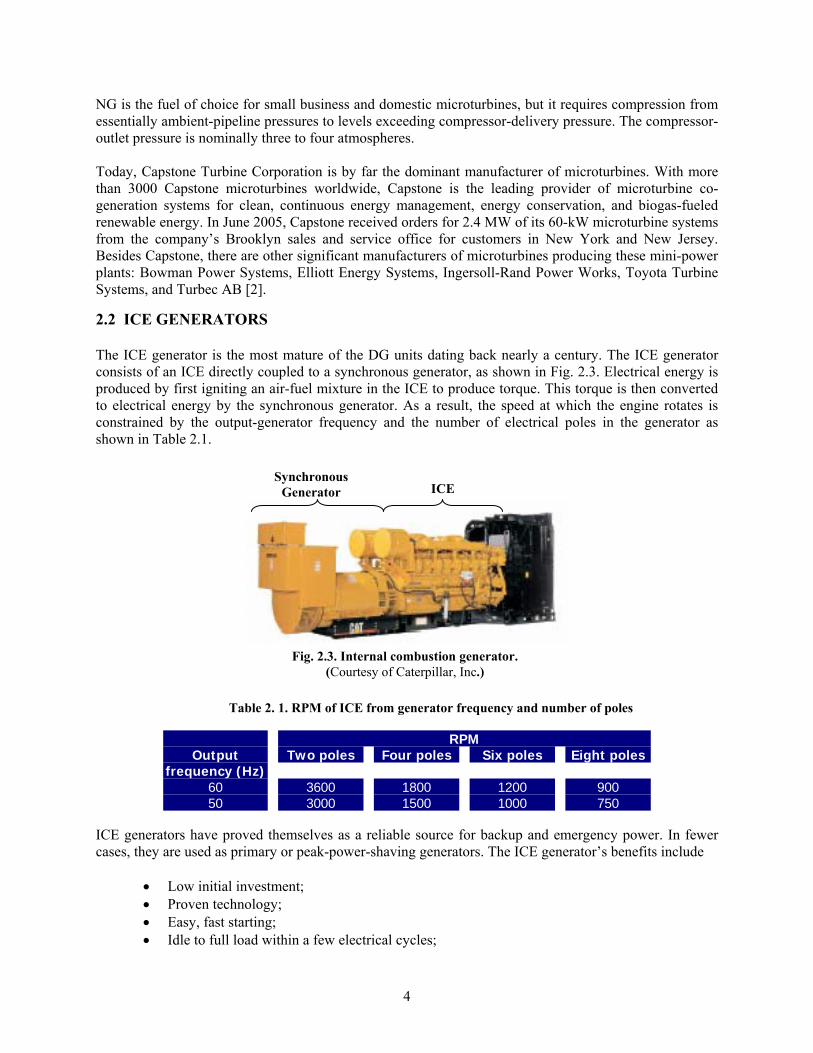
2.2 ICE GENERATORS The ICE generator is the most mature of the DG units dating back nearly a century. The ICE generator consists of an ICE directly coupled to a synchronous generator, as shown in Fig. 2.3. Electrical energy is produced by first igniting an air-fuel mixture in the ICE to produce torque. This torque is then converted to electrical energy by the synchronous generator. As a result, the speed at which the engine rotates is constrained by the output-generator frequency and the number of electrical poles in the generator as shown in Table 2.1.

Table 2. 1. RPM of ICE from generator frequency and number of poles

RPM Output

frequency (Hz) Two poles Four poles Six poles Eight poles

60 3600 1800 1200 900 50 3000 1500 1000 750

ICE generators have proved themselves as a reliable source for backup and emergency power. In fewer cases, they are used as primary or peak-power-shaving generators. The ICE generator’s benefits include

• Low initial investment; • Proven technology; • Easy, fast starting; • Idle to full load within a few electrical cycles;

Synchronous Generator ICE

Fig. 2.3. Internal combustion generator. (Courtesy of Caterpillar, Inc.)

5

• No power-electronics interface between generator and utility; and • Fast transfers from utility to island connect and back.

Their simplistic engineering, experienced service and maintenance personnel, readily available parts, and low-cost initial investment have ICE generators dominating the market for backup and emergency power. Commercial office buildings, hospitals, critical data centers, and manufacturing plants all rely on ICE generators to provide reliable backup and emergency generation. Generally, once a loss of utility power is detected, only a few cycles will be missed before the generator provides a full load.

The drawbacks of ICE generators are acoustic noise, NOX emissions, poor fuel efficiency, and frequent maintenance. Many urban areas have noise and emission ordinances; thus, ICE generators usually require noise suppression, environmental containment, and limited use during non-emergency conditions. The efficiency of ICE generators is 30–40% based on the amount of potential energy of the fuel and the output energy of the ICE. This low efficiency makes for costly operation during non-emergency or non-peak conditions. Maintenance requirements for ICE generators are the highest among all DG because of the many mechanical parts. These generators must be frequently operated (usually on a weekly basis) to ensure that they will start and run when called upon.

The fuels used in the ICE are primarily diesel, NG, methane gas, and gasoline. Diesel and gasoline are easily transported and stored on-site for use as demanded, while natural and methane gas ICEs must have a continuous supply from a reliable source and must be outfitted with appropriate plumbing. Historically, NG is less expensive than diesel; therefore, NG is used more frequently when available. A recent alternative fuel source for ICE generators is methane gas from landfill and wastewater treatment facilities. Methane gas is a free byproduct of coal seams, landfills, and wastewater treatment facilities during normal operation. Burning methane gas helps to lower the operating costs of a typical ICE unit making these units more attractive at these facilities.

ICE generators typically operate only a few hours per year consisting of maintenance, testing, and actual utility-power outages. Most standby generator sets are installed according to building code requirements and are designed to carry critical-electrical loads during outages. Facilities such as hospitals, critical data centers, and manufacturing plants often have substantial standby generation capacity. An estimate of approximately 40 GW of ICE generating capacity is installed in the United States, making these generators a key area of interest for ancillary services during non-emergency conditions [3].

Fig. 2.4. Internal combustion generator fueled by methane gas. (Courtesy of Cummins Power Generation)

Source: http://www.cumminspower.com/powerapplications/landfillgas.jhtml

6

2.3 SUMMARY ICE generators and microturbines are primarily operated as backup generation and peak-load sharing. ICE generators are the most mature of the DG units, where as microturbines are in their technical infancy. ICE generators are readily available in a wide variety of volt-amperes (VA) ratings, easy to install, and rapid start-up times. The drawbacks to these machines include the production of NOx and noise emissions that are harsh to the environment, low fuel efficiency, and high maintenance costs. Microturbines are machines that have higher fuel efficiency and take less real estate than ICE generators. The drawbacks to microturbines include more costly, higher maintenance, and slower startups than microturbines. A major difference between ICE generators and microturbines is that a microturbines’ electrical output is managed by power electronics. Power electronics are instrumental for providing multiple ancillary services described in the next chapter.

7

3. TYPES OF ANCILLARY SERVICES

Ten types of ancillary services are detailed in this report. Simple simulations have been conducted to demonstrate how each service might be provided. The ancillary services considered in this report include:

1. Voltage control, 2. Regulation, 3. Load following, 4. Spinning reserve, 5. Supplemental reserve (non-spinning), 6. Backup supply, 7. Harmonic compensation, 8. Network stability, 9. Seamless transfer, and 10. Peak shaving.

Reactive-power compensation is usually closely related with voltage control. However, because of its complexity and importance, the definition and compensation of reactive power is described separately in Chapter 4.

To provide the ancillary services from distributed energy resources (DER), the system should contain two subsystems: (1) the on-line detection subsystem, which detects the need for ancillary services and gives a signal when an ancillary service is needed; and (2) a function-realization subsystem, which works to provide the related ancillary services after receiving that signal. For example, the same DER could be a voltage supporter or a harmonics compensator. The only difference is in the control part; if the detection subsystem found the harmonics were beyond the pre-set range, it would start the control part of the harmonics compensator to let the DER work as a harmonics compensator. If the detection subsystem found the voltage to be beyond the pre-set range, then it would start the control part of the voltage supporter to let the DER operate as a voltage supporter. A control hierarchy must be established such that the DER provides the most important ancillary service when more than one ancillary service is needed. To decide which is the most important ancillary service, we need to consider both economical issues and technical feasibility. For most ancillary services, we need only additional software codes to provide it from DER. However, if an external energy-storage capability were available, the power converter could provide very high, short-duration power to start motors which is very important in providing ancillary services such as load following and regulation. Such external energy-storage devices may also be needed. 3.1 VOLTAGE CONTROL Voltage control is the injection or absorption of reactive power by generation and transmission equipment to maintain transmission-system voltages within required ranges or maintain the bus voltages of critical or sensitive loads; the latter is the emphasis of the discussion in this report [4]. Simulations will demonstrate how DER could perform the voltage-control function.

8

3.1.1 Voltage Control for Maintaining the Bus Voltage of Critical or Sensitive Loads There are three types of conditions that may cause voltage sag/swell for the bus voltage of critical or sensitive loads. The analysis scheme for voltage-control conditions is shown in Fig. 3.1:

• First condition: the load has some inductive component. The inductive component will not

absorb active power; however, it absorbs reactive power which will cause larger transmission-voltage drop and a lower load voltage VL.

• Second condition: the real power of the load changes. Changing the impedance value of the load could simulate this condition.

• Third condition: there is a fault in the utility that makes Vg change, so VL changes accordingly.

Fig. 3.1. System analysis scheme.

Generally speaking, the second and third condition may cause voltage sag or swell, and the first condition only causes voltage sag. 3.1.2 Control Methods Voltage control regulates the utility voltage to ensure it stays within a pre-set range. The system scheme for voltage support is shown in Fig. 3.2. The basic principle control is that if the voltage is smaller than the pre-set value, the DER will provide reactive power. If the voltage is larger than the pre-set value, DER will absorb reactive power.

There are at least three general control methods that can realize this basic principle:

1. Compare the actual root mean square (rms) value of VL and the reference value (for example,

480 V), then use the difference to control DER to provide/absorb reactive power. 2. Calculate the reactive power absorbed by the load and then use DER to provide it. The

calculation of reactive power is described in detail in Chapter 4. 3. Control DER to work as a voltage source that is in phase with VL but has different amplitude

from VL. Then the DER could provide/absorb reactive power. This will require some inductance between the DG and its utility interconnection so that the DG can control current flow to be in through the inductor (inductive) or out to the system (capacitive).

load

Utility Line

VL Vg

9

Fig. 3.2. System scheme for voltage support. When these methods are applied to DER control, the following point should be considered:

• Response time for DER with power electronics is on the order of milliseconds; and for DER without power electronics, response time is on the order of seconds.

3.1.3 Simulation Results for Control Method One A. Utility fault Use the following scheme (as shown in Fig. 3.3) to simulate a utility-fault condition: set rated voltage to be 4160 V. Choose [3952, 4368] to be a pre-set acceptable voltage range; when the voltage is outside this range, the voltage supporter is started. Change the amplitude of the ac voltage source to simulate the voltage-control effect.

Fig 3.3. Voltage-control system scheme for the first control method under utility-fault condition.

Figure 3.4 is the comparison between the compensated voltage (blue) and the original voltage (red) where the voltage before compensation is (a) 3620 V (13% less than the rated voltage), (b) 3229 V (22.4% less), (c) 2838 V (31.8% less), and (d) 2348 V (43.6% less). As shown in Fig. 3.5(a) and (b), the compensation effect is near ideal. However, when the utility fault is too severe, the resulting voltage may not be able to reach the pre-set value and the voltage wave may be distorted as shown in Fig. 3.4(c) and (d).

Load

Utility Line

VL Vg

DG (Working as

Voltage Supporter)

10

From Fig. 3.6, the current provided by DER is mostly reactive current only after about one cycle of dynamic process. Since the dynamic process is very short, DER will provide almost no energy in the dynamic process. In fact, the dynamic process shown in Fig. 3.6 is a function of the calculation period. It needs some time (1 cycle in this simulation, choosing TC = 1/60 s) to calculate the active and reactive current and, at the same time, the rms value of the voltage VL needs one cycle to be calculated in this simulation. From the simulation results we could see that, by comparing the rms value of V L to its expected value that controls the amount of provided reactive current, DER could support the voltage well under the condition resulting from utility fault. For voltage swell, take 5088 V (22.3% more than the rated voltage) as an example. Figure 3.5 is the comparison between the compensated voltage (blue) and the original voltage (red).

Take 3620 V (13% less than the rated voltage) as an example to show the active and reactive current provided by DER in this condition, which is shown in Fig. 3.6. The first plot is the entire current provided by DER, the second plot is the active component, and the third plot is the reactive component.

11

(b) Compensation effect when VL = 3229 V.

0 0.01 0.02 0.03 0.04 0.05 0.06 0.07 0.08 0.09 0.1-8000

-6000

-4000

-2000

0

2000

4000

6000

8000

t im e(s ec )

VL (

V )

V L w ith c om p

V L w ithout c om p

0 0.01 0.02 0.03 0.04 0.05 0.06 0.07 0.08 0.09 0.1-8000

-6000

-4000

-2000

0

2000

4000

6000

8000

tim e(s ec )

VL (

V )

V L with c om p

V L without c om p

0 0.01 0.02 0.03 0.04 0.05 0.06 0.07 0.08 0.09 0.1-8000

-6000

-4000

-2000

0

2000

4000

6000

8000

time(sec)

VL (

V )

VL with comp

VL without comp

0 0.01 0.02 0.03 0.04 0.05 0.06 0.07 0.08 0.09 0.1-8000

-6000

-4000

-2000

0

2000

4000

6000

8000

time(sec)

VL (

V )

VL with comp

VL without comp

(a) Compensation effect when VL = 3620 V.

(c) Compensation effect when VL = 2838 V. (d) Compensation effect when VL = 2348 V.

Fig. 3.4. Simulation results using Control Method One under grid-fault condition.

12

0 0.01 0.02 0.03 0.04 0.05 0.06 0.07 0.08 0.09 0.1-8000

-6000

-4000

-2000

0

2000

4000

6000

8000

time(sec)

VL (

V )

VL with comp

VL without comp

Fig 3.5. Compensation effect when VL = 5088 V.

0 0.01 0.02 0.03 0.04 0.05 0.06 0.07 0.08 0.09 0.1-1000

0

1000

time(sec)

i C (

A )

0 0.01 0.02 0.03 0.04 0.05 0.06 0.07 0.08 0.09 0.1-1000

0

1000

time(sec)

i Ca (

A )

0 0.01 0.02 0.03 0.04 0.05 0.06 0.07 0.08 0.09 0.1-1000

0

1000

time(sec)

i Cr (

A )

Fig. 3.6. Current provided by DER when VL = 3620 V. B. Inductive load

There are two techniques to simulate the inductive load as shown in Fig. 3.7. Generally, there is no difference between these two techniques because they are equal to each other under most conditions.

13

OR

(a) Series. (b) Parallel.

Fig. 3.7. Two techniques to simulate inductive load. However, when there are harmonic components in the current, these two load simulations are not equal. The simulation for this report used a parallel resistor inductor (RL) combination rather than a series RL combination. A filter will not be used to remove the harmonic components from DER in the simulation. If the series RL is used, the harmonic current will result in high-harmonics voltage (since jωL will become very high, if ω is very high); however, if parallel RL is used to simulate the inductive load, harmonic current will not have much influence.

Given R = 7.5 Ω and L = 50 mH as an example to simulate the inductive-load condition of power factor (PF) equal to 0.37. Figure 3.8 shows the simulation results. The first plot is the comparison of the voltage before (red) and after compensation (blue). The second plot is the total current provided by DER, the third plot is the active component, and the fourth plot is the reactive component. We could also see that the current provided by DER is mostly reactive current only after about one cycle of dynamic process.

0 0.01 0.02 0.03 0.04 0.05 0.06 0.07 0.08 0.09 0.1-1

0

1x 10

4

time(sec)

VL (

V )

0 0.01 0.02 0.03 0.04 0.05 0.06 0.07 0.08 0.09 0.1-1000

0

1000

time(sec)

i C (

A )

0 0.01 0.02 0.03 0.04 0.05 0.06 0.07 0.08 0.09 0.1-1000

0

1000

time(sec)

i Ca (

A )

0 0.01 0.02 0.03 0.04 0.05 0.06 0.07 0.08 0.09 0.1-1000

0

1000

time(sec)

i Cr (

A )

Fig. 3.8. Simulation results using Control Method One under the inductive-load condition.

Based on the simulation results, the technique of comparing the rms value of VL with the expected value to control the amount of provided reactive current, DER could support the voltage even with the inductive load.

14

C. Load change This simulation changes the resistant value of the load from 7.5 Ω to 4.5 Ω, which results in greater load current.

Figure 3.9 shows the simulation results. The first plot is the comparison of the voltage before and after compensation. The second plot is the entire current provided by DER, the third plot is the active component, and the fourth plot is the reactive component. As shown in Fig. 3.9, the current provided by DER is mostly reactive current only after about one cycle of dynamic process.

0 0.01 0.02 0.03 0.04 0.05 0.06 0.07 0.08 0.09 0.1-1

0

1x 10

4

time(sec)

VL (

V )

0 0.01 0.02 0.03 0.04 0.05 0.06 0.07 0.08 0.09 0.1-2000

0

2000

time(sec)

i C (

A )

0 0.01 0.02 0.03 0.04 0.05 0.06 0.07 0.08 0.09 0.1-2000

0

2000

time(sec)

i Ca (

A )

0 0.01 0.02 0.03 0.04 0.05 0.06 0.07 0.08 0.09 0.1-2000

0

2000

time(sec)

i Cr (

A )

Fig. 3.9. Simulation results using Control Method One with changes in the real power of the load.

Judging from the simulation results, we could see by comparing the rms value of VL and the expected value to control the amount of provided reactive current, that DER could support the voltage well when the real power of the load changes. 3.1.4 Simulation Results for Control Method Two with an Inductive Load Assume parallel RL load (R = 7.5 Ω and L = 15mH) to simulate the condition. Figure 3.10 shows the simulation results. The first picture is the comparison of the voltage before and after compensation. The second picture is the load current, the third picture is the active component of the load current, and the fourth picture is the reactive component. The fifth picture is the comparison of the load-reactive current and the current provided by DER and they match well from the comparison. Based on the simulation results, the technique of providing the reactive current in the load, DER could support the voltage well.

15

0 0 . 0 1 0 . 0 2 0 . 0 3 0 . 0 4 0 . 0 5 0 . 0 6 0 . 0 7 0 . 0 8 0 . 0 9 0 . 1-1

0

1x 1 0

4

t im e (s e c )

VL (

V )

0 0 . 0 1 0 . 0 2 0 . 0 3 0 . 0 4 0 . 0 5 0 . 0 6 0 . 0 7 0 . 0 8 0 . 0 9 0 . 1-2 0 0 0

0

2 0 0 0

t im e (s e c )

i L ( A

)

0 0 . 0 1 0 . 0 2 0 . 0 3 0 . 0 4 0 . 0 5 0 . 0 6 0 . 0 7 0 . 0 8 0 . 0 9 0 . 1-2 0 0 0

0

2 0 0 0

t im e (s e c )

i La (

A )

0 0 . 0 1 0 . 0 2 0 . 0 3 0 . 0 4 0 . 0 5 0 . 0 6 0 . 0 7 0 . 0 8 0 . 0 9 0 . 1-2 0 0 0

0

2 0 0 0

t im e (s e c )

i Lr (

A )

0 0 . 0 1 0 . 0 2 0 . 0 3 0 . 0 4 0 . 0 5 0 . 0 6 0 . 0 7 0 . 0 8 0 . 0 9 0 . 1-2 0 0 0

0

2 0 0 0

t im e (s e c )

i Lr(A

) an

d i Lc

(A)

Fig. 3.10. Simulation results using Control Method Two under the inductive-load condition.

3.1.5 Simulation Results for Control Method Three A. Utility fault The voltage is set to 97.75 V before compensation. Figure 3.11 shows simulation results using Control Method Three under a utility fault. The first plot is the comparison between the resulting voltage and the original voltage. The second plot is the whole current provided by DER, the third plot is the active component, and the fourth plot is the reactive component. The results indicate that the current provided by DER is mostly reactive current. Also, judging from the simulation results, the technique of DER acting as a voltage source with different amplitude and in phase with the utility, DER could support the voltage under the condition resulting from utility fault.

0 0.01 0.02 0.03 0.04 0.05 0.06 0.07 0.08 0.09 0.1-1

0

1x 10

4

time(sec)

VL (

V )

0 0.01 0.02 0.03 0.04 0.05 0.06 0.07 0.08 0.09 0.1-500

0

500

time(sec)

i C (

A )

0 0.01 0.02 0.03 0.04 0.05 0.06 0.07 0.08 0.09 0.1-500

0

500

time(sec)

i Ca (

A )

0 0.01 0.02 0.03 0.04 0.05 0.06 0.07 0.08 0.09 0.1-500

0

500

time(sec)

i Cr (

A )

Fig. 3.11. Simulation results using Control Method Three under a utility-fault condition.

16

B. Inductive load The results using a parallel RL (R = 7.5 Ω and L = 50 mH) to simulate the inductive load are shown in Fig. 3.12. The first plot is the comparison between the resulting voltage and the original voltage. The second plot is the whole current provided by DER, the third plot is the active component, and the fourth plot is the reactive component. The results indicate that the current provided by DER is mostly reactive current. Also, judging from the simulation results, the technique of DER acting as a voltage source with different amplitude and in phase of VL, it could support the voltage with an inductive load.

0 0.01 0.02 0.03 0.04 0.05 0.06 0.07 0.08 0.09 0.1-1

0

1x 10

4

time(sec)

VL (

V )

0 0.01 0.02 0.03 0.04 0.05 0.06 0.07 0.08 0.09 0.1-500

0

500

time(sec)

i C (

A )

0 0.01 0.02 0.03 0.04 0.05 0.06 0.07 0.08 0.09 0.1-500

0

500

time(sec)

i Ca (

A )

0 0.01 0.02 0.03 0.04 0.05 0.06 0.07 0.08 0.09 0.1-500

0

500

time(sec)

i Cr (

A )

Fig. 3.12. Simulation results using Control Method Three under an inductive load.

C. Change in real-power load Changes to the resistant value of the load from 7.5 Ω to 6.0 Ω would mean a heavier load. Figure 3.13 shows the simulation results. The first plot is the comparison of the voltage before and after compensation. The second plot is the whole current provided by DER, the third plot is the active component, and the fourth plot is the reactive component. The results indicate that the current provided by DER is mostly reactive current only after about one cycle of dynamic process.

From the simulation results, the technique of DER acting as a voltage source with different amplitude and in phase of VL, DER could support the voltage well under the condition that real power of the load changes.

3.1.6 Compensation Effect of the Three Control Methods under Severe-Voltage Sag As mentioned before, when the utility fault is too severe, the resulting voltage for Control Method One may not be able to reach the pre-set value and the voltage wave may be distorted. For inductive-load and load-change conditions, such a problem also exists. The most severe-voltage sag, which still could be compensated, depends on the control system’s parameters.

17

0 0.01 0.02 0.03 0.04 0.05 0.06 0.07 0.08 0.09 0.1-1

0

1x 10

4

time(sec)

VL (

V )

0 0.01 0.02 0.03 0.04 0.05 0.06 0.07 0.08 0.09 0.1-1000

0

1000

time(sec)i C

( A

)

0 0.01 0.02 0.03 0.04 0.05 0.06 0.07 0.08 0.09 0.1-1000

0

1000

time(sec)

i Ca (

A )

0 0.01 0.02 0.03 0.04 0.05 0.06 0.07 0.08 0.09 0.1-1000

0

1000

time(sec)

i Cr (

A )

Fig. 3.13. Simulation results using Control Method Three for real-power load changes.

For Control Method Two, such a problem does not exist. When Control Method Two is used, the exact reactive power needed always can be calculated, no matter how severe the voltage sag. The only limitation would be the current limit of the compensator.

For Control Method Three, DER is controlled as a voltage source in phase with VL but has different amplitude. When the voltage sag becomes severe, first the DER output voltage must increase and then the output-reactive power will be increased to support the voltage sag. At the same time, the output voltage must be in phase with VL so that output-active power is zero. Theoretically, the amplitude of the output voltage of the DER could be increased without limit; however, the compensator-current rating will provide a limit.

3.1.7 Voltage Control for Maintaining Transmission-System Voltages As mentioned before, there is another aim for voltage control, which is maintaining transmission-system voltages. As an example, Fig. 3.14 takes midpoint-voltage regulation of a transmission line connecting two generators.

x/2 x/2

Vs Vr

Ism Imr

s= sendingm=midpointr=receivingQ

P=0

Vm

Fig. 3.14. Midpoint-voltage regulation of a transmission line connecting two generators.

18

Assuming line impedance consists only of inductance X and Vs = Vr = V: • Without midpoint-voltage regulation, the permissible-power transfer from sending end to

receiving end is: srsrrs

sr XV

XVV

P δδ sinsin2

== , where δsr is < Vs – Vr.

• With reactive compensator at midpoint, Vs = Vm = Vr = V (same fundamental amplitude)

The compensator segments the line into two independent points: 1. From sending end to midpoint impedance = X/2. 2. From midpoint to receiving-end impedance = X/2.

Now by supplying only reactive power at midpoint:

2

sin2 2sr

sr XVP

δ= .

Thus, twice the rated power can transfer from bus s to bus r. From this example, by voltage control of the midpoint, the midpoint voltage is maintained to increase the permissible-power transfer. The basic principle of the control method is the same as voltage control for maintaining the bus voltage of critical or sensitive loads. 3.2 REGULATION Regulation is the use of online generation units that are equipped with governors and automatic generation control and can change in a timely fashion to regulate frequency [4]. When connected to a large bulk power system, a few megawatts of DER could do little to impact frequency. However, DER could perform this regulation function in a small island or microgrid [5].

When the mechanical power and electrical power of the synchronous generator are not in balance, then the frequency in the grid will change and the corresponding equation is

eumue

PPfH−=

⋅

ωπ4

,

where Pmu is the mechanical power (W), Peu is the electrical power (W), H is per unit inertia constant (s), ωe is the electrical-rotational speed, and f is the frequency, ωe = 2πf. Since f changes slightly, we could treat 4πH/ωe as a constant K. In our simulation let K = 50,000. Suppose that the load is in balance with generation supply before time t = 0 and the frequency is 60 Hz. At time t = 0, there is a step increase of 100 kW in the load power. DER shall supply this increased amount. Comparing the frequency with and without regulation, the result is shown in Fig. 3.15.

In Fig. 3.15, the first plot describes the comparison between load increment and the power DER provides. The second plot shows the comparison of the frequency with DER compensation and without DER compensation. In this simulation, the frequency could be controlled to be in the pre-set range (59.98–60.02 Hz) in less than one cycle (1/60 s).

19

0 0.01 0.02 0.03 0.04 0.05 0.06 0.07 0.08 0.09 0.10

50

100

150

200

time(sec)

P (

kW)

0 0.01 0.02 0.03 0.04 0.05 0.06 0.07 0.08 0.09 0.1 59.8

59.85

59.9

59.95

60 59.98

time(sec)

f (H

z)

compensated power

load increment

frequency without comp

frequency with comp

Fig. 3.15. Simulation results for the compensation effect for regulation.

3.3 LOAD FOLLOWING Figure 3.16 is the system scheme for load following. DG sells some of its power to the utility, while at the same time it supplies the load and tracks the changes in customer needs. For load following, part of the function is also to track the load, which is a similar control strategy to Control Method Two used earlier for voltage regulation. Load following is often mentioned together with regulation; they both address the temporal variations in load.

Fig. 3.16. System scheme for load following. In this system (providing ancillary services from DER), the difference between regulation and load following is that for load following DER sells some of its power to the utility and tracks the load’s change at the same time; but for regulation, DER only tracks the load’s change. However, in some of the other systems the distinction between load following and regulation is the time periods over which these fluctuations occur. Regulation responds to rapid-load fluctuations (on the order of one minute), and load following responds to slower changes (on the order of 5–30 minutes) [6]. So their precise definitions vary from system to system.

Load

Utility Line

V Vg

DG (Load following)

20

3.4 NETWORK STABILITY In trying to improve transmission-system use, a key assumption is that the existing system stability will be maintained. Network stability is the use of special equipment at a power plant (e.g., power system stabilizers or dynamic resistor) or on the transmission system (e.g., direct current (dc) lines, flexible ac transmission systems (FACTS), and energy storage) to help maintain transmission-system reliability [4]. For this example (providing ancillary services from DG), we mainly mention the latter instead of the former. To maintain network stability, power systems need to have adequacy which is defined as the ability of the power system to meet energy demands within component ratings and voltage limits. Energy storage can be used to enhance operation of the transmission-system power-flow control equipment by supplementing the ability of this equipment to generate or absorb active power [4]. Therefore, to maintain network stability, the energy-storage needs must be fully available very quickly (in the order of one cycle).

Network stability is similar to regulation, but it requires a more rapid response time. DER with power electronics could perform a network-stability function by monitoring frequency fluctuations and controlling the DER import/export since it can respond very quickly. As shown in Fig. 3.15, by using DER the frequency could be controlled to be in the pre-set range (59.98–60.02 Hz) in less than one cycle (1/60 s). However, since this ancillary service needs fast–responding ability, DER without a power-electronics interface could not perform it. It is important to note that simulations have been performed, and they indicate that in some cases DER inertia may destabilize the utility system. A likelihood is that their response to a system disturbance is dramatically phase shifted, causing a destabilizing effect possibly because the DER units are placed after significant level of reactance [7].

3.5 SPINNING RESERVE Normally, spinning reserve is the use of generating equipment that is online and synchronized to the grid so that the generating equipment can begin to increase output delivery immediately in response to changes in interconnection frequency and can be fully utilized within seconds to <10 minutes to correct for generation/load imbalances caused by generation or transmission outages [4]. Most on-line DER could supply spinning reserve and respond in less than 10 seconds.

For example, for DER with a power-electronics interface, the control method is to control the current from DER to let it be an active current and changing the amplitude of the current could change the output-active power of the DER. For DER without power electronics, DER must operate as a voltage source having the same amplitude as the user and a small leading-phase angle; controlling the phase angle controls the output-active power.

As an example, DER with a power-electronics interface will be simulated. Assume that at a time of 0.4 s, a frequency drop is detected and a decision is established to use DER to supply active power. The original source provides less active power and then the utility frequency is normal again. Figure 3.17 is the simulation result; the first plot is the active power and reactive power the source provides, the second plot is the active power and reactive power DER provides, and the third plot is the active power and reactive power the load absorbs.

From Fig. 3.17, the active power the source must provide changes from 1151 to 836 kW and the DER provides this difference (315 kW). Only about 0.02 s (from t = 0.04 s to t = 0.06 s) is needed for the

21

system to finish the dynamic process. Since 0.02 s is much smaller than 10 s, on-line DER is qualified as a spinning reserve.

0 0.02 0.04 0.06 0.08 0.1 0.12 0.14 0.16 0.18 0.20

1000

2000

time(sec)

PS (

kW)

0 0.02 0.04 0.06 0.08 0.1 0.12 0.14 0.16 0.18 0.20

500

1000

time(sec)

PC (

kW)

0 0.02 0.04 0.06 0.08 0.1 0.12 0.14 0.16 0.18 0.20

1000

2000

time(sec)

PL (

kW)

PSa

PSr

PCa

PSa

PLa

PCr

PLr

Fig. 3.17. Simulation results for spinning reserve.

3.6 SUPPLEMENTAL RESERVE (NON-SPINNING) Supplemental reserve (non-spinning) is the use of generating equipment and interruptible load that can be fully available to correct for generation/load imbalance caused by generation or transmission outages [4]. Supplemental reserve differs from spinning reserve because supplemental reserve need not respond to an outage immediately. Traditional non-spinning reserve needs to be available within 10 minutes.

If a DER system is not on-line, it needs some time to start.

• For a microturbine, using a Capstone microturbine as an example, approximately 120 s is

needed to start up. • For an ICE, the time needed to start is 2–5 s. • Most fuel cells (FCs) have a start-up time of 3–4 minutes.

For most DER, 10 minutes is adequate time to start and it is conceivable that an off-line DER system is appropriate to perform supplemental reserve. 3.7 PEAK SHAVING Peak shaving is the use of generation equipment during certain peak-load periods. Customers must purchase power at a higher cost during peak-load periods, and the demand charge is a function of the peak demand at any time during a year; therefore, use of generation for peak shaving can reduce a customer’s operational costs. DER could serve a peak-shaving function.

Peak shaving is providing active power to the user during peak load. It is also providing active power, which is similar to operating reserve in this point, so the accomplishment of the two ancillary services is

22

similar. However, operating reserve is a service given to the utility and peak shaving is a service given to the DER owner. 3.8 BACKUP SUPPLY Backup supply is a service that customers would purchase to protect against forced outages at the generating units that provide their energy or against loss of transmission between their normal supply and their load [4]. Unlike spinning reserve and supplemental reserve, which are system services required for reliability, backup supply is a commercial service that supports individual transactions. DER could perform backup supply. The basic principle is to use DER to supply the load during forced outages of the utility. The control method is to control the output voltage of the DER to give the load uninterruptible supply. For example, DER with power electronics is used in a simulation. The results are shown in Fig. 3.18 for four different cases. Figure 3.18(a) shows that for an outage that occurs at t = 0.0375 s when the current is at its peak amplitude (after 0.0001 s), the outage is detected and the DER begins to supply the load. The first plot is the current of the load and the second plot is the load voltage. In fact, this is the worst condition since the source voltage is lost when the current is at its maximum amplitude. Under this condition, DER needs approximately 0.083 s to supply the load normally.

Figure 3.18(b) shows that for an outage at t = 0.05s when the current is crossing through 0 after 0.0001 s, the outage is detected and the DER then starts to supply the load. Under this condition, there is almost no transition process and the DER could normally supply the load immediately. Figure 3.18(c) shows that for an outage at t = 0.04 s when the current is not 0 and not at the maximum amplitude after 0.0001s, the outage is detected and the DER starts to supply the load. Under this condition, there exists a transition; however, it is less than 0.0833 s.

Decreasing the value of the inductance that connects DER and the load may cause the transition process to be short and almost disappear; however, the voltage and current wave will not be as smooth as before. Take an outage that happens at t = 0.0375s as an example since this is the worst condition; the result is shown in Fig. 3.18(d). 3.9 HARMONIC COMPENSATION Harmonic compensation is the use of online generation equipment to compensate for harmonics caused by non-continuous loads. Harmonics can cause poor power quality, voltage imbalances, and excessive zero-sequence currents.

DER could perform a harmonic-compensation function. However, because harmonic compensation needs fast-response capability, DER without power-electronics interfaces cannot perform this function.

23

0 0.01 0.02 0.03 0.04 0.05 0.06 0.07 0.08 0.09 0.1-1000

-500

0

500

1000

time(sec)

i L ( A

)

0 0.01 0.02 0.03 0.04 0.05 0.06 0.07 0.08 0.09 0.1-1

-0.5

0

0.5

1x 10

4

time(sec)

VL (

V )

0 0 .01 0.02 0.03 0.04 0.05 0.06 0.07 0.08 0.09 0.1-1000

-500

0

500

1000

tim e(s ec )

i L ( A

)

0 0 .01 0.02 0.03 0.04 0.05 0.06 0.07 0.08 0.09 0.1-1

-0.5

0

0.5

1x 10

4

t im e(s ec )

VL (

V )

0 0.01 0.02 0.03 0.04 0.05 0.06 0.07 0.08 0.09 0.1-1000

-500

0

500

1000

time(sec)

i L ( A

)

0 0.01 0.02 0.03 0.04 0.05 0.06 0.07 0.08 0.09 0.1-1

-0.5

0

0.5

1x 10

4

time(sec)

VL (

V )

0 0.01 0.02 0.03 0.04 0.05 0.06 0.07 0.08 0.09 0.1-1000

-500

0

500

1000

t im e(s ec )

i L ( A

)

0 0.01 0.02 0.03 0.04 0.05 0.06 0.07 0.08 0.09 0.1-1

-0.5

0

0.5

1x 10

4

t im e(s ec )

VL (

V )

(b) Outage occurs at ts = 0.05 s. (a) Outage occurs at ts = 0.0375 s.

(c) Outage occurs at ts = 0.04 s. (d) Outage occurs at ts = 0.0375 s with less output inductance.

Fig. 3.18. Simulation results of the output current and voltage waveform for backup supply condition.

24

3.9.1 Harmonic Detection A. Circuit detection

Before harmonic-current compensation, harmonic current must be detected. A simple circuit is assumed to detect the fundamental current.

The detection circuit is shown in Fig. 3.19 with r = 0.9488 Ω, l = 35 mH, and C = 200 μF. For fundamental current, the impedance of this circuit is the largest; for harmonic currents the impedance is much smaller, almost negligible. Figure 3.20 is the impedance versus frequency measurement of this circuit.

Fig. 3.19. Fundamental current detection circuit.

Fig. 3.20. Impedance vs. frequency measurement of the RLC circuit in Fig. 3.19.

For the fundamental current (60 Hz), the impedance is more than 10 times that of the harmonics current. Since the original amplitude of the harmonics current is much smaller than that of the fundamental current, there is almost no harmonics voltage in the output voltage.

Z(jω)i

l

r

C

25

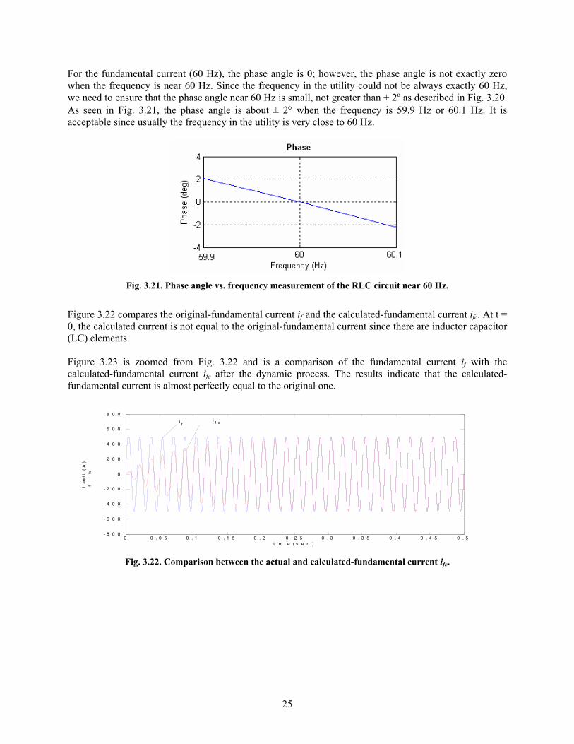
For the fundamental current (60 Hz), the phase angle is 0; however, the phase angle is not exactly zero when the frequency is near 60 Hz. Since the frequency in the utility could not be always exactly 60 Hz, we need to ensure that the phase angle near 60 Hz is small, not greater than ± 2º as described in Fig. 3.20. As seen in Fig. 3.21, the phase angle is about ± 2° when the frequency is 59.9 Hz or 60.1 Hz. It is acceptable since usually the frequency in the utility is very close to 60 Hz.

Fig. 3.21. Phase angle vs. frequency measurement of the RLC circuit near 60 Hz.

Figure 3.22 compares the original-fundamental current if and the calculated-fundamental current ifc. At t = 0, the calculated current is not equal to the original-fundamental current since there are inductor capacitor (LC) elements. Figure 3.23 is zoomed from Fig. 3.22 and is a comparison of the fundamental current if with the calculated-fundamental current ifc after the dynamic process. The results indicate that the calculated-fundamental current is almost perfectly equal to the original one.

0 0 . 0 5 0 . 1 0 . 1 5 0 . 2 0 . 2 5 0 . 3 0 . 3 5 0 . 4 0 . 4 5 0 . 5- 8 0 0

- 6 0 0

- 4 0 0

- 2 0 0

0

2 0 0

4 0 0

6 0 0

8 0 0

t i m e ( s e c )

i f and

i fc

( A

)

i fi f c

Fig. 3.22. Comparison between the actual and calculated-fundamental current ifc.

26

0 . 4 0 . 4 1 0 . 4 2 0 . 4 3 0 . 4 4 0 . 4 5 0 . 4 6 0 . 4 7 0 . 4 8 0 . 4 9 0 . 5- 8 0 0

- 6 0 0

- 4 0 0

- 2 0 0

0

2 0 0

4 0 0

6 0 0

8 0 0

t i m e ( s e c )

i f and

i fc(

A )

Fig. 3.23. Comparison between the actual if and calculated-fundamental current ifc after the dynamic process. B. Reactive-current calculation

Current detection is only one of the many methods for harmonics detection; others, for example, are reactive-current calculation and Fourier analysis.

Using reactive-current calculation as an example and using the reactive-current theory discussed in Chapter 4, choose Tc = 1/60s. The fundamental current is the active current, and the harmonic current is the reactive current. The calculated-active current will be the fundamental current. The comparison between the original-fundamental current and the calculated-fundamental current is shown in Fig. 3.24. The result shows that the calculated-fundamental current is perfectly equal to the original after only one calculation period Tc = 0.0167 s.

0 0 . 0 1 0 . 0 2 0 . 0 3 0 . 0 4 0 . 0 5 0 . 0 6 0 . 0 7 0 . 0 8 0 . 0 9 0 . 1- 8 0 0

- 6 0 0

- 4 0 0

- 2 0 0

0

2 0 0

4 0 0

6 0 0

8 0 0

t i m e ( s e c )

i f and

i fc(

A )

i f ci f

Fig. 3.24. Comparison between the actual if and calculated-fundamental current ifc using reactive-current theory.

3.9.2 Harmonic Compensation The principle for harmonic compensation is to (1) calculate the fundamental current if from the load current iL, then (2) subtract if from the load current iL to get the harmonic current, which is the ic that the compensator should provide as shown in Fig. 3.25.

27

ic

iLiS

loadcompensator

Source

ic

iLiS

loadcompensator

Source

Fig. 3.25. Harmonic-compensation schematic diagram.

Figure 3.26 is the compensation result. The first plot shows the load current iS1 (before compensation) and the fundamental current if. The second plot shows the load current iS2 (after compensation) and the fundamental current if. The third plot shows the calculated harmonic current ih and the compensated harmonic current ic.

0.35 0.4 0.45 0.5

-500

0

500

(a)

i S1 a

nd i f (

A )

time(sec)

time(sec)

time(sec)

0.35 0.4 0.45 0.5

-500

0

500

(b)

i S2 a

nd i f (

A )

0.35 0.4 0.45 0.5-200

0

200

(c)

i h and

i c ( A

)

Fig. 3.26. Simulation results for harmonic compensation.

3.10 SEAMLESS TRANSFER When DER transfers from stand-alone mode to utility-connection mode, or vice-versa, it is expected to transfer almost instantaneously; the operation is called “seamless transfer.” In a wider definition, seamless transfer is the ability for online generation to transition among various ancillary services without power-delivery disruption. Here we assume the former definition and discuss how DER could perform seamless transfer. The following is a summary of a paper by Tirumala et al. [8].

3.10.1 Requirements of the Control Algorithm Figure 3.27 shows the interconnection of the pulse-width modulation (PWM) inverter to the utility. The critical load is connected across the output of the PWM inverter at the point of common coupling (PCC).

28

To be able to disconnect from the utility in the least possible time, a triac is used as a static-transfer switch (STS). The triac would ensure that the utility can be disconnected from the load within half a line-frequency cycle in the event of a fault.

Fig. 3.27. Interconnection of the PWM inverter to the utility [8].

The PWM inverter is operated in current-controlled mode when it is connected to the utility and it regulates the current injected into the PCC. The utility is assumed to be relatively stiff and maintains the voltage across the load. In the stand-alone mode, the PWM inverter is operated in the voltage-controlled mode. The inverter is controlled to regulate the voltage across the load. Thus, the PWM inverter has to be capable of shifting between current-controlled and voltage-controlled modes to maintain the voltage across the load in the presence of faults on the utility.

The control algorithm required to transfer between current-controlled and voltage-controlled modes should ensure that the STS turns off before the inverter shifts to the voltage-controlled mode (otherwise, it will result in two voltage sources being connected in parallel). Also, the algorithm has to ensure that the voltage applied across the load matches the load voltage just before disconnect so that there are no inrush currents drawn by the load as a result of the sudden change in the load voltage.

For the transfer between voltage-controlled and current-controlled mode, the inverter voltage should match the utility voltage in both magnitude and phase (synchronize) before the STS can be turned on (the triac should be turned on when there is essentially zero voltage across it). Once the triac is turned on, the utility current should be slowly ramped up to prevent any voltage spikes caused by the grid inductance.

The proposed algorithm takes care of all the above-mentioned requirements associated with the transfer of a PWM inverter between grid-tied and off-grid modes. Moreover, the algorithm is completely independent of the actual realization of the current and voltage controllers.

3.10.2 Utility–Interactive Mode to Stand–Alone Mode Assume initially that the inverter is operating in the grid-tied mode. The PWM inverter is current-controlled, and the utility governs the voltage at the PCC. When there is a fault on the utility, the voltage at the PCC drops. The fault-detection circuitry turns off the triac when the utility voltage drops below a pre-set minimum value. Thus, the inverter is disconnected from the utility at the first zero crossing of the utility current after the triac has been turned off. At this instant, the PWM inverter can be shifted from current-controlled to voltage-controlled mode.

If the load is a motor-type load or if the fault on the utility is not shorted at the load, the voltage at the PCC will not drop to zero instantaneously but will decay exponentially. Figure 3.28 shows the polar plot of the voltage for the case of a motor-type load, with decaying magnitude and varying phase. In such a case, when the inverter is shifted to voltage-controlled mode, it is necessary to match the magnitude and phase of the voltage at the PCC to avoid high-inrush currents. By using a digital-signal processor (DSP)

29

to monitor the voltage at the PCC, it is possible to measure the magnitude and phase of the load voltage at the instant of utility disconnect. These values form the starting magnitude and phase of the voltage reference given to the voltage controller. The voltage magnitude is then ramped up from the initial value to the rated value in the span of a couple of line cycles. Thus the steps to be performed in the algorithm can be summarized as follows.

1. Detect a fault on the utility and give a turn-off signal to the triac. 2. Monitor the magnitude and phase of the load voltage. 3. When the triac current goes to zero, switch the inverter to a voltage-controlled mode with the

voltage reference being derived from the load voltage. 4. Ramp up the magnitude of the load voltage from its initial value to the rated value.

Fig 3.28. Polar plot of the load voltage [8]. 3.10.3 Stand-Alone Mode to Utility-Interactive Mode Assume initially that there is a fault on the utility and the inverter is operating in voltage-controlled mode with the STS open. When the fault on the utility is cleared and the utility voltage comes back on, the phase and amplitude of the load voltage (maintained by the PWM inverter) and the utility voltage may not match. Thus, before the triac can be turned on to reconnect the inverter to the utility, the magnitudes and phases of the two voltages must be matched. The magnitudes can be matched easily by ramping the inverter-reference voltage up or down to match the utility voltage. However, in order to match the phase, it is necessary to increase or decrease the frequency of the load voltage until the phases match.

To determine the change in the frequency of the load voltage required to obtain a phase match in the shortest time, a simple function can be used. Figure 3.29 plots the change in the load-voltage frequency required (Δ f) as a function of the phase of the load voltage that is measured at the rising-edge zero crossing of the utility voltage. A phase measurement of zero or 2π indicates that the two voltages are in phase. Thus at these values, the required Δ f is zero, and hence the function is tapered to zero. This also ensures that once a phase match is obtained, the two voltages stay in phase.

One possible problem with the function shown in Fig. 3.29 is the jitter that can occur if the phase is close to π. In this case, depending on the errors in measurement, Δ f will oscillate between +1 and −1, locking

30

the two voltages out of phase permanently. This situation can be avoided by having a small hysteresis around π as shown in Fig. 3.30.

Fig. 3.29. Δ f as a function of Φload [8].

Fig. 3.30. Δ f as a function of Φload (with hysteresis) [8].

Once the phase and amplitude match is obtained, the PWM inverter is shifted from the voltage-controlled mode to the current-controlled mode. Similar to the previous case, the current reference of the PWM inverter at the instant of turn-on of the triac is matched to the load current. The inverter current is then slowly changed to match the pre-specified current injection into the utility. Thus the steps to be performed in this phase of the algorithm can be summarized as follows:

1. Detect that the utility is within nominal operating parameters. 2. Adjust the load voltage to match the magnitude and phase of the utility voltage. 3. Once load voltage is equal to utility voltage, turn on the triac and switch from voltage-

controlled to current-controlled mode, with the reference current being equal to the load current.

4. Change the reference current slowly to the desired current (both magnitude and phase).

31

3.10.4 Simulation Results Simulation of the proposed algorithm was carried out in SABER [9] for a 120-V, 750-VA single-phase PWM inverter system. An average-current controller and a voltage controller were designed. The parameters of the system are

Inverter rated output voltage: 120 V Inverter rated output VA: 750 VA Load: 350 VA at 0.8pf lag Load current (rms): 2.96 A Initial utility current (rms): 3.45A

A. Grid-tied mode to off-grid mode Figures 3.31 and 3.32 show the simulation results for a transfer from a grid-tied mode to an off-grid mode.

Fig. 3.31. Grid current during grid-tie mode to off-grid mode transition.

32

Fig. 3.32. Voltages during grid-tie mode to off-grid mode transition. The utility voltage starts reducing at approximately 0.18 s. Once the utility voltage reaches about 80% of its steady-state value, a turn-off signal is applied to the gate of the triac. The triac turns off at the next zero crossing of the utility current (Fig. 3.31).

As can be seen from Fig. 3.32, the voltage across the load is continuous at the time of disconnect from the utility and the controller starts the inverter voltage in both amplitude and phase match with the utility. The load voltage is slowly ramped up to the rated value in about five line cycles. Figure 3.33 shows the load current, which does not have any inrush spikes during the entire transition period, indicating a smooth transition from current-controlled mode to voltage-controlled mode.

Fig. 3.33. Load current during grid-tie mode to off-grid mode transition.

33

B. Off-grid mode to grid-tied mode Figure 3.34 shows the utility voltage and inverter-output voltage during the phase-match stage. The voltages start out 180° out of phase and reach phase match in about 0.5 s.

Fig. 3.34. Load and utility voltages during phase-match transition.

Figure 3.35 shows the frequency change (Δ f) during this time. The value is found to start at one and gradually decrease to zero.

Figure 3.36 shows the load voltage and grid current when the triac is turned on. The grid current is slowly ramped up so that there are no spikes in the load voltage because of the line inductance. The load voltage is found to be smooth during the entire transition period.

Fig. 3.35. Variation in Δ f with time.

34

Fig. 3.36. Load voltage and utility current when the triac activates. 3.11 SUMMARY

This chapter describes the ten types of ancillary services that can be provided by DER. Simple simulations have been conducted to demonstrate how each service might be provided. An alteration of software code is needed to provide most of the ancillary services; however, if an external energy storage capability was available, the power converter could provide very high, short-duration power to start motors, which is very important in providing ancillary services such as load following and regulation. Such external energy storage devices may also be needed.

35

4. REACTIVE POWER Reactive (or nonactive) power compensation is closely related to voltage control. There are many definitions of nonactive power/current. There is little debate about the definitions of active power or nonactive power in sinusoidal cases, but the theories differ in the case of non-sinusoidal and non-periodic waveforms. Some definitions work well in three-phase, three-wire systems but are not able to handle the single-phase case; others can be applied only to periodic waveforms. Some definitions are physical quantities, while others do not have any physical meanings.

The theory proposed by Peng and Lai [10] is a generalized theory of instantaneous-active power/current and instantaneous-nonactive power/current for a three-phase system. Active power is the time rate of energy generation, transmission, or consumption. The current that carries active power is the active current, which is the component of current in phase with the voltage. Nonactive power is the time rate of the energy that circulates back and forth between the source and load. In a multi-phase circuit, it also includes the power that circulates between phases.

4.1 STANDARD DEFINITIONS FOR REACTIVE POWER 4.1.1 Ideal Electric-Power System Ac, three-phase electric-power systems were developed in the late 1800s and have been adopted as the standard for more than 100 years. In an ideal power system, the voltage and current are sinusoidal at a constant frequency (50 Hz or 60 Hz) and balanced (the same magnitude for each of the three phases, and the phase angle between consecutive phases being 120° radians). A system is considered ideal if the generation is ideal (sine wave with constant magnitude and constant-fundamental frequency) and all the loads are linear. (The loads consist only of resistance R, inductance L, and/or capacitance C.) There are single-phase loads (two-wire), three-phase loads (three-phase without neutral), and three-phase, four-wire loads (three-phase with neutral) in ac power systems.

4.1.2 Standard Definitions For an ideal electric-power system as defined above, the standard definitions are as follows [11]: f denotes the frequency and T = 1/f is the period; v(t) denotes the instantaneous voltage for which a typical sinusoidal waveform has the form

)cos(2)( tVtv ω= . (4.1)

The instantaneous current is denoted by i(t) and a typical sinusoidal waveform has the form

)cos(2)( θω += tIti , (4.2) where ω = 2πf and θ is the phase angle between v(t) and i(t). V and I are the rms values of the voltage v(t) and the current i(t) over the time T, respectively; that is

2

0

1 ( )T

V v t dtT

= ∫ (4.3)

and

36

∫=T

dttiT

I0

2 )(1. (4.4)

The instantaneous power p(t) is defined by

)()()( titvtp = . (4.5) The instantaneous power p(t) is, at the terminals of entry into a delimited region, the rate at which the electric energy is being transmitted by the circuit into or out of the region [11]. For a multi-phase system, define the voltage vector v(t) by

1 2( ) [ ( ), ( ),..., ( )]Tmt v t v t v t=v . (4.6)

The current vector i(t) is defined by

1 2( ) [ ( ), ( ),..., ( )]Tmt i t i t i t=i , (4.7)

where m is the number of the phases. The instantaneous power p(t) is defined by

∑=

==m

kkk

T titvtitvtp1

)()()()()( . (4.8)

The definitions in Eqs. (4.5) and (4.8) are also true for voltages and currents with arbitrary waveforms.

The average active power P over the time period T is the average value of the instantaneous power over one period of the waveform; that is

∫=T

dttpT

P0

)(1. (4.9)

In the case of a sinusoidal voltage and current as given in Eqs. (4.1) and (4.2) respectively, it follows that

0

1 ( ) cosT

P p t dt VIT

θ= =∫. (4.10)

The apparent power is defined by

VIS = . (4.11) The average reactive power is defined by

22 PSQ −= . (4.12) The power factor pf is defined by

37

SPpf = . (4.13)

If the voltage and current are sinusoidal and are as given in Eqs. (4.1) and (4.2) respectively, then cospf θ= .

4.2 GENERALIZED REACTIVE-POWER THEORY 4.2.1 Nonlinear Loads and Distortion in Power Systems Because of generation, transmission, and nonlinear loads in a power system, there are distortion and deviation in the voltage and/or current waveforms which deteriorate the quality of the electric power. For example, the harmonics generated in the system may be amplified because of parallel and series resonance in the system. The existence of harmonics reduces the energy efficiency of a power system at the generation, transmission, and consumption points of the system. Harmonics can cause extra heating of the cores of transformers and electrical machines. Furthermore, the harmonics may expedite the aging of the insulation of the components in the system and shorten their useful lifetimes.

In a system with distortion in the current and voltage waveforms, the standard definitions given for reactive power and reactive current are no longer applicable to defining, measuring, or describing the power quality which is a precondition to improve the power quality as well as to eliminate the distortion in the system. Different reactive-power theories have been proposed in the literature, and different reactive-power compensation methods have been implemented to compensate the reactive-power component in a power system. In this report, a new approach is presented on instantaneous reactive-power definitions which can be used in a reactive-power compensation system for fundamental reactive power and other reactive power as well.

4.2.2 Generalized Reactive-Power Theory The theory presented here is based on Fryze’s idea of nonactive power/current [12] and is an extension of the theory proposed in [13]. It is independent of the number of phases of the system. The definitions in the previous subsection are based on a single-phase system. In a multi-phase system, the voltage and current are vectors which are defined by

v(t) = [v1, v2,…, vm]T (4.14) and

i(t) = [i1, i2,…, im]T (4.15) where m is the number of phases. The instantaneous-active current ia(t) and the instantaneous-nonactive current in(t) are defined by

ia(t))(

)(2 TV

tP

P

= vp(t) (4.16)

and

38

in(t) = i(t) – ia(t). (4.17) The reference voltage is given by

1 2( ) [ , ,..., ]Tp p pmt v v v=pv . (4.18)

The rms value of vp(t) is then defined by

1( ) ( ) ( ) c

tT

pc t T

V t dT

τ τ τ−

= ∫ p pv v. (4.19)

The instantaneous power p(t) is the summation of the instantaneous power of each phase

p(t) = vT(t)i(t) =∑=

m

kkk titv

1

)()( . (4.20)

The average power P(t) over time period [t-Tc, t] is

∫−

=t

Ttc c

dpT

tP ττ )(1)(. (4.21)

In particular, for a three-phase system with

[ ]1 2 3( ) ( ) ( ) ( ) Tt v t v t v t=v (4.22) and

[ ]1 2 3( ) ( ) ( ) ( ) Tt i t i t i t=i , (4.23) the instantaneous-active current and the instantaneous-nonactive current are, respectively,

1 1

2 22

3 3

( ) ( )( )( ) ( ) ( )( )

( ) ( )

a p

a pp

a p

i t v tP tt i t v t

V ti t v t

⎡ ⎤⎡ ⎤⎢ ⎥⎢ ⎥= = ⎢ ⎥⎢ ⎥⎢ ⎥⎢ ⎥⎣ ⎦ ⎣ ⎦

ai (4.24)

1 1 1

2 2 2

3 3 3

( ) ( ) ( )( ) ( ) ( ) ( )

( ) ( ) ( )

n a

n a

n a

i t i t i tt i t i t i t

i t i t i t

⎡ ⎤ ⎡ ⎤ ⎡ ⎤⎢ ⎥ ⎢ ⎥ ⎢ ⎥= = −⎢ ⎥ ⎢ ⎥ ⎢ ⎥⎢ ⎥ ⎢ ⎥ ⎢ ⎥⎣ ⎦ ⎣ ⎦ ⎣ ⎦

ni (4.25)

where

39

[ ]1 1 2 2 3 31( ) ( ) ( ) ( ) ( ) ( ) ( )

c

t

c t T

P t v i v i v i dT

τ τ τ τ τ τ τ−

= + +∫ (4.26)

and

2 2 21 2 3

1( ) ( ) ( ) ( ) c

t

p p p pc t T

V t v v v dT

τ τ τ τ−

⎡ ⎤= + +⎣ ⎦∫ . (4.27)

For a three-phase, four-wire system, the neutral current i0(t) is the sum of the other three phases; i.e.,

)()()()( 3210 titititi ++= . (4.28)

The instantaneous-active power pa(t) and the instantaneous-nonactive power pn(t) are, respectively,

[ ]1

1 2 3 2 1 1 2 2 3 3

3

( )( ) ( ) ( ) ( ) ( ) ( ) ( ) ( ) ( ) ( ) ( )

( )

a

a a a a a

a

i tp t v t v t v t i t v t i t v t i t v t i t

i t

⎡ ⎤⎢ ⎥= = + +⎢ ⎥⎢ ⎥⎣ ⎦

(4.29)

and

[ ]1

1 2 3 2 1 1 2 2 3 3

3

( )( ) ( ) ( ) ( ) ( ) ( ) ( ) ( ) ( ) ( ) ( )

( )

n

n n n n n

n

i tp t v t v t v t i t v t i t v t i t v t i t

i t

⎡ ⎤⎢ ⎥= = + +⎢ ⎥⎢ ⎥⎣ ⎦

. (4.30)

Unlike many of the other nonactive-power/current definitions, the above definitions do not put any limitations on the voltage v(t) and current i(t) waveforms. It is a general definition independent of the number of phases and whether voltages or currents are sinusoidal or non-sinusoidal and periodic or non-periodic. For each different case, it is consistent with the traditional definitions. It takes on a specific form by choosing the reference voltage vp(t) and the averaging interval Tc. This will be elaborated upon in the following sections.

4.2.3 Reference Voltage vp(t) and Averaging Interval Tc The reference voltage vp(t) is used to specify the shape of the instantaneous-active current waveform. Choices for vp(t) include

1. vp(t) = v(t), if v(t) is a pure sinusoid or the active current ia(t) is preferred to have the same

waveform as v(t). 2. vp(t) = vf(t), where vf(t) is the fundamental component of v(t). In power systems, if v(t) is

distorted or even unbalanced and a purely sinusoidal ia(t) is desired, then vp(t) is chosen as the fundamental positive-sequence component of v(t). This ensures that ia(t) is balanced and does not contain any harmonics, even if the source voltage is distorted or unbalanced.

By choosing different reference voltages, ia(t) can be reshaped and the unwanted components in i(t) can be eliminated. Furthermore, the elimination of each component is independent of the other.

40

The averaging time interval Tc can be chosen arbitrarily from zero to infinity and for different Tc, the resulting active current will have different characteristics. Case 1: Tc = 0 In this case, instead of averaging over the period Tc, the system variables are specified instantaneously; that is

( ) ( )( ) ( )( ) ( )

T

T

t tt tt t

=av ii vv v (4.31)

( ) ( ) ( ) ( ) ( ) ( )T T

ap t t t t t p t= = =av i v i (4.32)

( ) ( ) ( ) 0Tnp t t t= =nv i . (4.33)

So, if Tc = 0, the instantaneous-nonactive power is zero and the instantaneous-active power is equal to the instantaneous power p(t). Case 2: Tc is a finite value For a periodic system with harmonics only, Tc is chosen as Tc = T/2 or T, where T is the fundamental period. For a system with subharmonics containing frequencies that are not an integral multiple of the fundamental frequency, a longer Tc is required to completely eliminate the nonactive component. Case 3: Tc → ∞ In power systems, the system voltage is sinusoidal with low-harmonic distortion (the total harmonic distortion is less than 5%); therefore, a non-periodic system indicates that only the current is non-periodic. A sinusoidal-active current can be achieved only if Tc is infinite (P(t)/V2

p(t) is constant). In practice, it is not possible to implement a compensation system in which Tc is infinite. Usually Tc is chosen to be 1–10 times the fundamental period based on the tradeoff between acceptable compensation results and reasonable capital cost. Table 4.1 shows the different combinations of vp and Tc for different nonlinear loads, and the corresponding compensation results are shown in the last column.

41

Table 4.1. Summary of the parameters vp and Tc in the nonactive-power theory

Load current i(t) vp Tc Active current ia(t)

Tc 0 Three-phase fundamental nonactive current

v

T/2 or T

Unity pf and pure sine wave

v T/2 or T Unity pf and same shape of v

vf+ T/2 or T Pure sine wave and in phase with vf+.

Single-phase or multi-phase fundamental nonactive current and harmonic current

v Tc → 0 Instantaneous current

Nonperiodic disturbance current vf+ nT Reduced amplitude and near sine wave with unity pf

Subharmonic current vf+ nT Pure sine wave or smoothed sine wave with unity pf

Nonperiodic current vf+ nT Smoothed sine wave with unity pf

Nonperiodic current v ∞ In phase with v

Notes: Both v(t) and i(t) are distorted except in Case 1.. vf+ is the positive sequence of the fundamental component of v.

4.2.4 Simulation Results This simulation takes a three-phase, four-wire unbalanced load as an example. Most loads in a power system are three-phase. If there is a neutral line and the load is unbalanced, there will be a neutral current flowing in the neutral line. A three-phase, four-wire system is balanced if the phase angle between each of the two phases is 120° and all the phases have the same magnitude; otherwise, it is unbalanced. Harmonics are the most common distortion in power systems, existing in both voltage and current. Harmonics compensation is independent of the averaging interval Tc if Tc is an integer multiple of T/2. According to the definition of active current:

)()(

)()( 2 tvtVtPti p

Pa = .

For harmonics compensation, P(t) and Vp(t) are constant; i.e., ip(t) is in phase with vp(t) and has the same waveform as vp(t) when Tc is an integer multiple of T/2. If the system voltage is not distorted and the load current has harmonics and is unbalanced, then the system voltage itself can be used as the reference voltage to achieve sinusoidal, balanced, and unity power-factor source current after compensation.

If the system voltage is also distorted, choosing a different reference voltage will result in a different source current. If the source current in the previous case is still preferred, another reference voltage should be used other than the system voltage which is usually the positive sequence ( 1v+ ) of the fundamental component of the system voltage vs. The source currents will be sinusoidal and balanced, and the system will have a unity PF. This case is illustrated in Fig. 4.1.

42

(a) System voltage vs(t)

(b) Load current il(t)

(c) vsa(t) and reference voltage vpa(t)

(d) Reference voltage vp(t)

(g) Source neutral current isn(t)

(h) dc-link voltage vdc(t)

Fig. 4.1. Simulation results of compensating unbalanced load harmonics with distorted-system voltage. If the system voltage itself is used as the reference voltage vp(t), is(t) will be proportional to and have the same shape as vs(t) as shown in Fig. 4.2. The blue waveforms are the system voltages (phase 1, 2, and 3 respectively, which are scaled by a factor of 5 for clearness) and the red waveforms are the source currents after compensation, which have the same shape as the system voltages [14].

(a) vsa(t) and isa(t); (b) vsb(t) and isb(t); (c) vsc(t) and isc(t).

Fig. 4.2. Distorted-source current after compensation if vp = Vs is chosen.

4.3 SUMMARY This chapter describes the standard and instantaneous definitions for reactive power. The differences are pronounced by distortion in the current and voltage waveforms; where as the standard definitions given for reactive power and reactive current are no longer applicable. In section 4.2.4, the simulation shows distorted source currents can be compensated using injected reactive current to yield a pure sinusoidal waveform. The system then will have a unity PF.

43

5. TYPES OF ANCILLARY SERVICES PROVIDED FROM DER Not every DER has a power-electronics interface. Generally speaking, DER without a power-electronics interface can provide fewer types of ancillary services because it cannot respond as quickly as DER with a power-electronics interface.

5.1 DER WITH POWER-ELECTRONICS INTERFACE There are two main types of power-electronics topologies for DER to be connected to the utility. One is for DER whose output is ac voltage; the other is for DER whose output is dc voltage. Take as examples a microturbine with ac output voltage and a FC with dc output voltage.

5.1.1 Power-Electronics Interface for a Microturbine The most common power-converter topology used for connecting microturbines to the utility is the dc-link converter. Figure 5.1 shows a microturbine generator feeding power to an active rectifier circuit (or, alternatively, a passive rectifier) followed by a dc link and inverter circuit.

Fig. 5.1. Simplified diagram of a dc-link converter.

The high-frequency power from the generator must be converted to dc before the inverter can reconstruct a three-phase voltage supply at the lower frequency required for utility connection. A controller manages the operation of the active rectifier and inverter circuitry by ensuring that functions such as voltage following, current following, phase matching, harmonic suppression, and so on are performed reliably and at high efficiency.

The controller may be mostly on-board, personal computer (PC)-based, a processor linked to a PC, etc. depending on constraints and factors such as desired microturbine packaging, desired versatility, type of available features, and the sophistication/maturity of the system design [14].

5.1.2 Power-Electronics Interface for a FC Since most FC modules operate in the voltage range of 25–45 Vdc and the utility voltage is 230 Vrms. The power-electronics interface must perform two tasks: the power must be inverted and the voltage must be amplified. As shown in Fig. 5.2, these tasks could be done either by connecting an inverter to the FC

44

followed by a 60-Hz transformer (ac-to-ac voltage gain) or by connecting a switch mode dc-to-dc converter to the FC ( dc-to-dc voltage gain) followed by a utility-connected inverter. A dc-to-dc voltage gain (switch mode dc-to-dc converter) is preferred in order to limit the physical size and the cost of the system [16].

Fig. 5.2. Schematic description of the power inverter for a FC. 5.1.3 Control of DER with a Power-Electronics Interface From the discussion above, we see that normally there is a dc-to-ac inverter in the power-electronics interface for DER to be connected to the utility. By controlling the dc-to-ac inverter, DER with power electronics could provide the 10 types of ancillary services as discussed earlier in Chapter 3. At the same time, energy should be supplied from the DER to make the dc voltage constant.

There are mainly two controls needed: control of the dc-to-ac inverter to provide the ancillary service immediately and regulation of the dc-link voltage of the inverter. The PWM inverter is operated in current-controlled mode when it is connected to the utility and regulates the current injected into the PCC. In stand-alone mode, the PWM inverter is operated in voltage-controlled mode. The inverter is controlled to regulate the voltage across the load.

Most of these ancillary services operate in current-controlled mode since they are under utility -connection conditions. For backup supply, DER operates in voltage-controlled mode because it is under stand-alone mode. Furthermore, for seamless transfer, DER transfers from stand-alone to utility-connection mode or from utility-connection to stand-alone mode. Thus, the PWM inverter has to be capable of shifting between current-controlled and voltage-controlled modes to maintain the voltage across the load in the presence of faults on the utility.

For some ancillary services, the DER needs to provide only reactive power, such as voltage control and harmonics compensation; for some other ancillary services, the DER needs to provide active power such as regulation, load following, operating reserve, backup supply, network stability, and peak shaving.

To provide reactive power, the inverter must provide a current whose phase is 90° lagging or leading the load voltage. When it is 90° leading, the reactive power provided is negative, or the inverter is absorbing reactive power. When it is 90° lagging, the reactive power provided is positive, or we can say the inverter is supplying reactive power. In order to produce the 90° phase difference between the utility voltage and current supplied by the inverter, we let the output voltage of the DER be in phase with the source voltage but with a different amplitude than the load voltage. By inserting an inductance between the output

FC Inverter dc-to-ac

Voltage Gain ac-to-ac

Utility

FC Inverter dc-to-ac

Voltage Gain ac-to-ac

Utility

(a) Voltage gain in ac-to-ac stage.

(b) Voltage gain in dc-to-dc stage.

45

voltage of the DER and the source voltage (see Fig. 3.2), then the current through the inductance will be a current whose phase is 90° lagging or leading the load voltage.

For voltage control, there are three methods to control the voltage to rated voltage as mentioned before. Since the DER with power electronics could respond quickly, it could support the voltage in a very short time.

For harmonic compensation, first calculate the harmonic current that must be compensated and then output this current. The calculation of the harmonic current must be precise and quick, and this is a concern for the two methods that have been mentioned in the report (circuit detection and reactive-current calculation). Another concern in harmonic compensation is providing the harmonic current immediately; this could be accomplished only by DER with power electronics because DER without power electronics cannot respond quickly enough.

To provide active power for such services as load following, operating reserve, network stability, and peak shaving the inverter needs to provide a current in phase with the load voltage. The current’s amplitude is determined by the local and system demand. Details can be found in Chapter 3. For backup supply, the DER acts in a stand-alone mode so it only needs to control the output voltage.

5.1.4 DER without a Power-Electronics Interface Some microturbine makers choose not to use power electronics but instead use a speed-reduction gear between the turbine and alternator that produces fixed-frequency and -voltage three-phase output. In addition, for traditional generator sets with ICEs, there is no power-electronics interface between generator and utility.

Without a power-electronics interface, DER cannot provide those ancillary services that require a fast response time, such as harmonic compensation and network stability. But for the other ancillary services, DER without a power-electronics interface can provide them.

As an example of Control Method One for voltage control, the control principle is to compare the rms value of VL and the expected value (for example, 480 V), then use the difference to control the DER to provide/absorb reactive power. Both DER with a power-electronics interface and DER without a power-electronics interface could perform this principle. However, after the rms value of VL and the expected value are compared to get a difference value, the DER with power electronics can provide the required reactive power very quickly and the DER without power electronics cannot respond as fast, and its response to dynamic system changes may be unsatisfactory. 5.2 SUMMARY

This chapter describes the types of ancillary services provided from DER with and without a power-electronics interface. Microturbine and FC are used to show the structure of the power-electronics interface of DER. The control methods to provide different ancillary services are also mentioned. Without a power-electronics interface, DER cannot provide those ancillary services that require a fast response time, such as harmonic compensation and network stability. DER without a power-electronics interface can provide the other ancillary services.

46

6. TYPES OF ANCILLARY SERVICES THAT PROVIDE THE BEST IMPACT 6.1 WHY PROVIDE ANCILLARY SERVICES FROM DER Even a few years back, the main concern of consumers of electricity was the reliability of the supply. Even though the power generation in most advanced countries is fairly reliable, the distribution is not always so.

A power outage is the loss of the electricity supply to an area, and unscheduled outages cause major problems to both utilities and customers alike. The reason for a power failure can be, for instance, a defect in a power station, damage to a power line or other part of the distribution system, a short circuit, or the overloading of electricity mains. Sometimes it is caused by natural disasters and accidents like earthquakes, floods, blizzards, tornadoes, fires, arson, or terrorist activities. A power outage may be referred to as a blackout if power is lost completely as a voltage sag, if some power supply is retained but the voltage level is below the minimum level specified for the system or as a voltage swell if the voltage level is above the maximum level specified for the system. A voltage sag is usually more common than voltage swell [17].

Power outages cause higher financial loss to utility customers arising from loss of production in factories and assembly lines and rotting or contamination of edible materials in food processing plants, restaurants, and even domestic households. The impact of even short outages in semiconductor plants can be very severe [17].

Power failures are particularly damaging for hospitals, since many life-critical medical devices and tasks require power. For this reason, hospitals like many enterprises (notably collocation facilities and other data centers), have emergency power generators that are typically powered by diesel fuel and configured to start automatically as soon as a power failure occurs. Other life-critical systems such as telecommunications are also required to have emergency power [17].

There are many loads that cannot tolerate voltage sags, such as adjustable-speed drives (ASDs), computers, and programmable logic controllers. ASDs are used in many process industries. If these drives stop because of voltage sags, the result may be the termination of the process in which these drives are employed. That may in turn result in a reduction in the quality of the product or the loss of raw material that cannot be used again. Therefore, these undesirable events must be avoided [18].

While ancillary services provided by DER perhaps could not have prevented past large-scale blackouts, a large penetration of these devices throughout the electric grid might protect against a future large-scale electric catastrophe. The following is a list of recent well-known, wide-scale power outages [17]:

• During the California electricity crisis, there were regular power failures resulting from

energy shortages and market manipulation resulting from failed deregulation. • On August 14, 2003, there was a wide-area power failure in the northeastern United States

and central Canada that affected 50 million people (see 2003 North America blackout). • On August 28, 2003, there was a blackout in London that prompted worldwide headlines

(e.g., “Power cut cripples London”) but in fact only affected 500,000 people. • On September 23, 2003, a power failure affected five million people in Denmark and

southern Sweden. • On September 27–28, 2003, a power failure affected all of Italy except Sardinia, cutting

service to more than 56 million people. • On December 20, 2003, a power failure hit San Francisco affecting 120,000 people.

47

• On September 4, 2004, five million people in Florida were without power at one point as a result of Hurricane Frances, one of the most widespread outages ever due to a hurricane.

• On May 25, 2005, most parts of Moscow were without power from 11:00 MSK (+0300 UTC). Approximately 10 million people were affected. Power was restored within 24 hours.

Harmonics is another major concern for utilities. Although most electronic equipment in our professional environment makes work more convenient, these devices complicate demands on facility wiring and power utilities. Most facilities employ a variety of devices such as multiple-switch mode power supplies, motors, fans, and other nonlinear loads. Among the adverse effects of multiple-nonlinear loads are voltage distortion, excessive neutral return currents, reduced utilization of available power, and power-factor penalties.

Harmonic currents in particular are receiving more attention as a critical power-quality concern, with an estimated 40% of electricity now passing through nonlinear loads. Ironically, the equipment used to boost productivity and efficiency is also generating increases in non-productive power consumption, power pollution, and low-PF. Additionally, the equipment producing the harmonic distortion is also highly susceptible to its damaging effects [19].

The symptoms of harmonic-voltage distortion can be severe and serious problems can result:

• Transformers may overheat, cables may get too hot, and the insulation may break down.

Capacitors may overheat or form tuned circuits that resonate [20]. • The presence of harmonics can cause additional losses in induction motors, especially when

they are operating close to their rated values. Moreover, as a result of the additional losses created by harmonic currents, overall heating may increase leading to premature failure of the motors [18].

• Electronic displays and lighting may flicker, circuit breakers may trip, fuses may blow spuriously, computers may fail, and metering may give false readings [20].

• The supply voltage is used for timing purposes in many cases. For example, supply-voltage cycles are counted to get timing information for digital clocks. Similarly, many items of power electronic equipment, such as phase-controlled thyristor circuits, use the zero crossing of the supply voltage to generate trigger pulses for semiconductor devices. A distorted voltage waveform can create false triggering of the timing circuits [18].

• Most office buildings contain many items sensitive to excessive harmonic distortion, such as computers, and these must be protected from the harmful effects.

Since these power-quality problems bring so much loss to utility users, ancillary services must be provided to solve them. What is more, utilities need to carry operating reserve to ensure adequate system performance and to guard against sudden loss of generation, off-system purchases, unexpected load fluctuations, or unexpected transmission-line outages. The discussion of operating reserves so far has emphasized their use to protect against major generation and transmission outages, a form of insurance intended to help maintain bulk-power reliability. In practice, utilities have historically used operating reserves for additional reliability and commercial purposes [21].

Providing ancillary services from DER will be a good solution to power-quality problems, which could be seen from the following points:

• Local regulation is much more efficient with local sources and DER can supply precisely the

level of regulation needed [5]. Here “regulation” means not only the regulation of voltage

48

(voltage support as mentioned in Chapter 3), but also the regulation of frequency (network stability, load following, and regulation as mentioned in Chapter 3). So DER is a good fit to provide voltage control, network stability, load following, and regulation.

• Harmonic compensation and network stability both require fast-response capability; DER with power electronics is appropriate to provide these two ancillary services.

• DER is perfect to provide backup supply and peak shaving because of their proximity to the user. In fact, DG applications today are primarily designated for backup and peak power-shaving conditions.

• DER could serve as reserve to the utility and perform other ancillary services when the utility has enough power. So there will be no waste for the resource.

6.2 COST TO PROVIDE ANCILLARY SERVICES Although providing ancillary services from DER has great economic benefits, its cost must also be considered. Sandia National Laboratories prepared a report in 1998 that detailed the costs for power converters associated with energy-storage systems [22].

The power-conversion system (PCS) cost was broken into four major cost centers—power stage, device drivers, PCS controller, and balance of system (BOS). The power stage consists of the topological connection of switching devices, its thermal management, and its protective circuits (such as snubbers). The nameplate rating of the power stage (which includes the ratings of its semiconductor devices and ancillary circuits), the chosen inverter topology, and the control requirements are all factors that determine the overall cost of the inverter. The device drivers are circuits that take input signals from the controller and affect the turn-ON/turn-OFF of the switching devices. The PCS controller includes the inner loop, outer loop, and fictional-control loop. The BOS includes the dc interface, the ac interface, and the magnetics.

6.2.1 PCS Costs for Various Ancillary Services PCS companies were contacted and estimated cost structures were discussed. The companies interviewed were asked to provide the total cost of the PCS which includes materials, labor, and overhead. Switchgears, transformers, and cabinets are also included in the total PCS cost. Shipping and installation costs are not included in the total PCS cost because they are site-specific and highly variable.

• PCS costs for voltage-regulation applications Three companies discussed PCS costs for voltage-regulation applications, but only two provided cost breakdown information. As shown in Table 6.1, the total cost for a voltage-regulation application ranges from $150–500/kW. The power stage accounted for 33–36% of the total PCS cost, the controller for 10–33%, and the BOS for 33–54%. Both companies that gave detailed information (Companies A and B) included the cost of the device drivers in the power-stage costs.

Table 6.1. PCS costs for voltage-support applications

Company Total $/kW

Power stage (% reduction)

Device drivers (% reduction)

Controllers (% reduction)

BOS (% reduction)

A $400 33% (−30%) In PS 33% (−30%) 33% (−30%) B $500 36% (−30 to 40%) In PS 10% (−33%) 54% (ROI1) C $150 NA NA NA NA

1 Return on investment.

49

The cost-reduction potential for the power-stage/device drivers ranged from 30–40% of the current cost. The companies also saw a potential 30–33% reduction in the cost of controllers. Company A estimated a 30% reduction could be achieved for the BOS; however, Company B felt that the cost for the BOS fluctuated with the rate of inflation. • PCS costs for peak-shaving applications The same three companies supplied cost information for the customer demand peak-reduction application, but only two provided cost breakdown information. The total PCS cost for this application ranged from $420–750/kW, as shown in Table 6.2. Both of the companies that provided detailed cost information (Companies A and B) included the cost of the device drivers in the power-stage costs, which accounted for 32–36% of the total PCS cost. The controller accounted for 10–30% of the total PCS cost, and the BOS for 10–30%.

Table 6.2. PCS costs for peak-shaving applications

Company Total $/kW

Power stage (% reduction)

Device drivers (% reduction)

Controllers (% reduction)

BOS (% reduction)

A $420 32% (−30%) In PS 32% (−30%) 36% (−30%) B $500 36%(−30 to 40%) In PS 10% (−33%) 54% (ROI1) C $750 NA NA NA NA

1 Return on investment. Companies A and B speculated that a 30–40% reduction in power-stage costs could be achieved. It was anticipated that the lower cost, solid-state switches coming on the market could result in such a reduction. The cost-reduction potential for controllers was estimated as being between 30 and 33%. Company A estimated a 30% reduction in BOS costs in the near future; however, Company B stated that BOS costs, and consequently any potential cost reductions, depend on the rate of inflation. For example, the cost of steel used for enclosures fluctuates according to the rate of inflation, as does the cost of copper and iron used in filters and transformers.

• PCS costs for area control/frequency regulation applications The cost estimates and cost-reduction potentials for PCSs used in area control/frequency regulation applications were highly speculative and presented a wide cost range (see Table 6.3). Company A estimated the total PCS cost for this application as $320/kW, while Company B estimated only $80/kW. Both costs are based on low-volume production, and in both estimates the cost of the device drivers was combined with the power-stage cost. The device drivers and power stage accounted for 40–44.5% of the total PCS cost. The controller accounted for 4.7–6% and the BOS from 50.8–54%.

Table 6.3. PCS costs for voltage-support applications

Company Total $/kW

Power stage (% reduction)

Device drivers (% reduction)

Controllers (% reduction)

BOS (% reduction)

A $320 44.5% (−30%) In PS 4.7% (−30%) 50.8% (−30%) B $80 40%(−30 to 40%) In PS 6% (−33%) 54% (ROI1)

1Return on investment. Company A suggested that a 30% cost reduction could be achieved for the power stage, controller, and BOS. This reduction is based on high-volume production, which tends to reduce cost. Company B indicated that a 30–40% reduction was possible for the power stage and device drivers based on the

50

possible availability of higher rated components in the near future. The use of higher rated components would reduce the need for protective circuits for a high-power system and consequently reduce the costs associated with supplying those circuits. Company B sees a possible 33% cost reduction in controller technology, primarily based on moving toward digital circuits from older, more expensive, analog circuits. Company B stated that because the BOS costs fluctuate with the rate of inflation, they are unpredictable [22].

6.2.2 Cost Reduction Recommendations • Higher component integration and increased functionality Higher component integration and increased functionality per unit area—such as that which could be achieved by replacing analog components with digital components in controller circuits—could also result in cost reductions as well as a smaller package. The sophisticated internal processes, such as self-testing, in digital controllers simplify controller maintenance and diagnostics. Digital circuits also require fewer calibrations and less testing and set-up time compared with analog circuits.

As mentioned in Chapter 3.9, there are two methods for the detection of harmonics: analog circuits and digital calculation. Based on this consideration, the latter should be preferred. Furthermore, with the development of DSP technology, the response time could satisfy most of the conditions now. • Use of advanced semiconductors Some cost reductions may also be realized from advances in semiconductors. Insulated gate bipolar transistors (IGBTs) are leading today’s market for semiconductors used in medium-level (up to 750-kVA) PCSs [23]. IGBT technology has wide industry support and is most likely to provide the greatest cost-reduction potential for the near future. Advanced semiconductors have increased switching speeds that allow for higher operating frequencies, which in turn reduce the size of filters and other passive components. Increases in semiconductor voltage and current ratings could also reduce the number of switches required for higher rated systems while improving reliability and reducing design complexity. Fewer semiconductor switches would reduce the need for protective circuits (such as snubbers) and elaborate heat-sink designs, thus reducing the overall cost. Nevertheless, higher rated components will help reduce cost only to a certain degree. Three-phase operation, for instance, will still require at least six semiconductor switches for a converter.

Recently, silicon carbide (SiC)-based power devices have been drawing increasing attention because of their superior characteristics compared with silicon (Si)-based power devices. SiC-based power devices possess the features of high voltage, high power, high frequency, and high-temperature operation in a smaller package. An SiC-based power converter would have the benefits of reduced losses, higher efficiency, a reduction of up to 2/3 in the heat-sink size, smaller passive components, and less susceptibility to extreme ambient heat [14].

• Modular-component designs Possibly the greatest cost reduction in PCS development would come from combining modular-semiconductor switching devices with advanced microprocessor controllers. The trend in industry appears to be toward modular-component designs that use advanced controllers; for example, some manufacturers are placing the entire inverter-power stage in a single package with one heat sink. This standardization of a single, modular package that could be used for a variety of applications by slightly modifying the software could reduce or eliminate the need for custom-designed PCSs. Modular design tends to reduce

51

noise sensitivity in components and reduce electromagnetic interference (EMI), but it has a tendency to require increased complexity in the heat sinks used in the devices. This modular concept is currently being pursued by the federal interagency Power Electronics Building Block program.

As shown in Tables 6.1, 6.2, and 6.3, the cost for the controller is a relatively small cost among the PCS’s four cost components. If the same power stage, device drivers, and BOS can be used and a different controller used to realize different ancillary services, as mentioned in the introduction of Chapter 3, then the cost for providing ancillary services from DER will be tremendously reduced.

The potential cost reductions discussed require design enhancements that can increase the initial design cost of the PCS. However, the costs of PCS components and subassemblies are generally on a downward trend. Advances in technology are expected in the areas of packaging, semiconductors, and power-conversion topologies. These advances may help reduce the number of parts required and the size of the units and, combined with increased demand and higher production will probably result in lower PCS costs in the future. Finally, most manufacturers agreed that they would like to see reductions in the costs of the magnetic components (e.g., transformers and filter inductors) and do not feel that much work is being done in this area [22].

6.3 BEST IMPACT OF ANCILLARY SERVICES By the goal of the ancillary services, these 10 types of ancillary services could be divided into those that mostly benefit the utility, those that mostly benefit the DER owner, and those that benefit both more or less equally.

6.3.1 Providing the Most Impact to the Utility Spinning reserve, supplemental reserve (non-spinning), and network stability provide the most impact to the utility. All three of these ancillary services aim to keep the load and supply in balance, which keeps the frequency of the utility at its normal value (60 Hz) so they are system services required for reliability and provide the most impact to the utility.

6.3.2 Providing the Most Impact to the DER Owner Backup supply, peak shaving, load following, and seamless transfer provide the most impact to the DER owner.

Backup supply is a service that customers would purchase to protect against forced outages at the generating units that provide their energy, or against loss of transmission between their normal supply and their load. Thus, backup supply is a commercial service that supports individual transactions and provides the most impact to the DER owner.

Peak shaving is the use of generation equipment during certain peak-load periods. Customers must purchase power at a higher cost during peak-load periods; therefore, use of generation for peak shaving can reduce customers’ operational costs. Thus, peak shaving provides the most impact to the DER owner.

Load following is the use of online generation equipment to track the changes in customer needs. This minimizes the power purchased from the utility. Thus, load following provides the most impact to the DER owner.

When DER transfers from stand-alone mode to utility-connection mode or from utility-connection to stand-alone mode, it is expected to transfer seamlessly. By providing uninterrupted service to a company’s loads, seamless transfer provides the most impact to the DER owner.

52

6.3.3 Provide the Most Impact to Both the Utility and the DER Owner Voltage control, regulation, and harmonic compensation impact the utility and the DER owner more or less equally.

Voltage control regulates a bus voltage which improves the power quality of the DER owner, but it also minimizes reactive power drawn from the utility, improving system efficiency and stability.

For regulation, the goal is to maintain the rated frequency of the utility by tracking the load’s demand. The DER owner is also a part of the load, so regulation provides impact to both the utility and the DER owner.

Through harmonic compensation, the source avoids the need to provide harmonic current to a load with harmonic components because it has been provided by the DER. Thus, there will be no harmonic current flowing through the rest of the utility. This improves system efficiency and stability by reducing losses in the rest of the system. It may also enable the owner of a harmonic-producing load to avoid paying penalties to the utility for harmonic-producing loads that do not comply with IEEE 519, “Harmonics Control in Power Systems.”

6.4 SUMMARY This chapter described the needs and costs associated with ancillary services, as well as cost reducing recommendations. These ten types of ancillary services could be divided into the following three categories: (1) those that mostly benefit the utility, (2) those that mostly benefit the DER owner, and (3) those that benefit both more or less equally. Spinning reserve, supplemental reserve (non-spinning), and network stability provide the most impact to the utility; backup supply, peak shaving, load following, and seamless transfer provide the most impact to the DER owner; voltage control, regulation, and harmonic compensation impact the utility and the DER owner more or less equally.

Higher component integration and increased functionality, use of advanced semiconductors, and modular component designs are all recommendations to reduce the system costs. Only then, DER can be economical for a large penetration of these devices throughout the electric grid which might protect against future large-scale electric catastrophes.

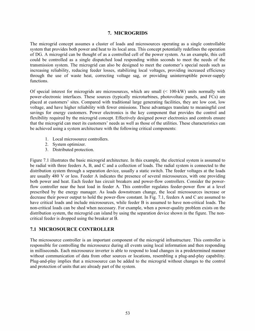
53

7. MICROGRIDS The microgrid concept assumes a cluster of loads and microsources operating as a single controllable system that provides both power and heat to its local area. This concept potentially redefines the operation of DG. A microgrid can be thought of as a controlled cell of the power system. As an example, this cell could be controlled as a single dispatched load responding within seconds to meet the needs of the transmission system. The microgrid can also be designed to meet the customer’s special needs such as increasing reliability, reducing feeder losses, stabilizing local voltages, providing increased efficiency through the use of waste heat, correcting voltage sag, or providing uninterruptible power-supply functions. Of special interest for microgrids are microsources, which are small (< 100-kW) units normally with power-electronic interfaces. These sources (typically microturbines, photovoltaic panels, and FCs) are placed at customers’ sites. Compared with traditional large generating facilities, they are low cost, low voltage, and have higher reliability with fewer emissions. These advantages translate to meaningful cost savings for energy customers. Power electronics is the key component that provides the control and flexibility required by the microgrid concept. Effectively designed power electronics and controls ensure that the microgrid can meet its customers’ needs as well as those of the utilities. These characteristics can be achieved using a system architecture with the following critical components:

1. Local microsource controllers. 2. System optimizer. 3. Distributed protection.

Figure 7.1 illustrates the basic microgrid architecture. In this example, the electrical system is assumed to be radial with three feeders A, B, and C and a collection of loads. The radial system is connected to the distribution system through a separation device, usually a static switch. The feeder voltages at the loads are usually 480 V or less. Feeder A indicates the presence of several microsources, with one providing both power and heat. Each feeder has circuit breakers and power-flow controllers. Consider the power-flow controller near the heat load in feeder A. This controller regulates feeder-power flow at a level prescribed by the energy manager. As loads downstream change, the local microsources increase or decrease their power output to hold the power-flow constant. In Fig. 7.1, feeders A and C are assumed to have critical loads and include microsources, while feeder B is assumed to have non-critical loads. The non-critical loads can be shed when necessary. For example, when a power-quality problem exists on the distribution system, the microgrid can island by using the separation device shown in the figure. The non-critical feeder is dropped using the breaker at B.

7.1 MICROSOURCE CONTROLLER The microsource controller is an important component of the microgrid infrastructure. This controller is responsible for controlling the microsource during all events using local information and then responding in milliseconds. Each microsource inverter is able to respond to load changes in a predetermined manner without communication of data from other sources or locations, resembling a plug-and-play capability. Plug-and-play implies that a microsource can be added to the microgrid without changes to the control and protection of units that are already part of the system.

54

Fig. 7.1. Microgrid architecture [24].

7.1.1 Basic Control of Real and Reactive Power There are two basic classes of microsources: dc and ac. Dc sources consist of FCs, photovoltaic cells, and battery storage while ac sources consist of ICEs and high-frequency microturbines, which need to be rectified. In both cases, except for the ICE, the resulting dc voltage is converted to an acceptable ac source using a voltage-source inverter. Shown in Fig. 7.2 is the general model for a microsource containing three basic elements: prime mover, dc interface, and voltage-source inverter. The voltage-source inverter provides control of both the magnitude and phase of its output voltage, V. The vector relationship between the inverter voltage, V, and the system voltage, E, along with the inductor’s reactance, X, determines the flow of real and reactive power (P and Q) from the microsource to the system.

Fig. 7.2. Interface-inverter system [24].

The P and Q magnitudes are coupled as shown in Eqs. (7.1), (7.2), and (7.3). For small changes, P is predominantly dependent on the power angle, δP, while Q is dependent on the magnitude of the

55

converter’s voltage, V. These provide for basic feedback loops for the control of output power and bus voltage, E, through regulation of reactive-power flow.

PXVEP δsin

23

= , (7.1)

)cos(23

PEVXVQ δ−= , and (7.2)

EVP δδδ −= . (7.3)

7.1.2 Voltage Regulation through Droop Cooperation among large numbers of microsources is not practical with basic P-Q controls. Voltage regulation is necessary for local reliability and stability. Without it, systems with high penetration of microsources can experience voltage and/or reactive-power oscillations. Voltage control requires care to ensure that there are not large circulating-reactive currents between sources. In the power grid, the impedance between large generators is usually enough to greatly reduce the possibility of circulating currents. However, in a typically radial microgrid large circulating-reactive currents cannot be ignored. Small errors in voltage set-points can result in a circulating current that can exceed the ratings of the microsources. This situation requires a voltage versus reactive-current droop controller. The local voltage set-point is reduced as the reactive current generated by the microsource becomes more capacitive. Conversely, as the current becomes more inductive, the voltage set-point is increased [24]. The function of the basic controller is shown in Fig. 7.3. The Q limit shown in the figure is a function of the VA rating of the inverter and the power being provided by the prime mover.

Fig. 7.3. Voltage set-point with droop [24].

7.1.3 Fast Load Tracking and the Need for Storage A system with groups of microsources and storage could be designed to operate both in an isolated mode and connected to the power grid. In isolated operation, load-tracking problems arise since microturbines and FCs have slow response and are inertia-less. The prime movers’ output power time constants range from 10–200 s, which is too slow for most loads. Recall that the present power systems have storage provided though the generator’s inertia. When a new load comes on line, the initial energy balance is satisfied by the system’s inertia. This results in a slight reduction in system frequency. A system with

56

clusters of microsources designed to operate in an island mode must provide some form of storage to ensure initial energy balance. The necessary microgrid storage can come in several forms: batteries or supercapacitors on the dc bus for each microsource, direct connection of ac storage devices (batteries, flywheels, etc.), or use of traditional generation with inertia with the microsources. If the microgrid is not required to operate in island mode, the energy unbalance can be met by the ac system without providing storage on the microgrid.

7.1.4 Frequency Droop for Power Sharing Microgrids provide premium power through the ability to smoothly move from dispatched power mode (while connected to the utility grid) to load tracking (while in island mode). In the island mode, such problems occur as slight errors in frequency generation at each converter, and the need to change power operating points to match load changes using power versus frequency-droop functions at each microsource without an explicit communication network.

In grid-connected mode, the loads in the microgrid receive power both from the grid and from the microsources. In case of loss of the grid due to voltage drops, faults, and blackouts, the microgrid smoothly transfers to island operation. With separation from the grid, the voltage-phase angles at each microsource in the microgrid change, resulting in an apparent reduction in local frequency. This frequency reduction, coupled with a power increase, allows for each microsource to provide its proportional share of load without new power dispatch from the energy manager. In island operation, the energy manager is not used except for reconnection to the grid.

Consider two microsources, as suggested in Fig. 7.4. In this example, the sources are assumed to have different ratings, P1max, and P2max. The dispatched power in grid mode (P01 and P02) is defined at base frequency, ω0. The droop is defined to ensure that both systems are at rated power at the same minimum frequency.

Fig. 7.4. Power vs. frequency-droop control [2].

During a change in power demand, these two sources operate at different frequencies which causes a change in the relative-power angles between them. As this happens, the two frequencies tend to drift toward a lower, single value, ω1. Unit 2 was initially operating at a lower power level than Unit 1. However, at the new power level, Unit 2 has increased its share of the total power needs. Although power is adjusted within fractions of seconds, frequency restoration can take longer. A restoration function must be included in each controller. The droop-control design is based on each microsource having a maximum

57

power rating. As a consequence, droop is dependent on the dispatched power level while the microsources are connected to the grid.

7.2 SYSTEM OPTIMIZATION The energy manager provides system optimization. The energy manager uses information on local electrical and heat needs, power-quality requirements, electricity and gas costs, wholesale/retail service needs, special grid needs, demand-side management requests, and congestion levels to determine the amount of power that the microgrid should draw from the distribution system. Some key functions of the energy manager are

• Provide the individual power and voltage set-point for each power flow and microsource

controller. • Ensure that heat and electrical loads are met. • Ensure that the microgrid satisfies operational contracts with the transmission system. • Minimize emissions and system losses. • Maximize the operational efficiency of the microsources. • Provide logic and control for islanding and reconnecting the microgrid during events.

7.3 PROTECTION Protection must respond to both system and microgrid faults. If the fault is on the utility grid, the desired response may be to isolate the microgrid from the main utility as rapidly as necessary to protect its loads. The speed of isolation is dependent on the specific customer’s loads on the microgrid. In some cases, sag compensation can be used without separation from the distribution system to protect critical loads. If the fault is within the microgrid, the protection coordinator isolates the smallest possible section of the radial feeder to eliminate the fault. Most conventional distribution protection is based on short-circuit current sensing. Power electronic-based microsources cannot normally provide the levels of short circuit required. Microsources may be capable only of supplying twice the load current or less to a fault. Some overcurrent sensing devices will not even respond to this level of overcurrent, and those that do respond will take many seconds to respond, rather than the fraction of a second that is required.

The unique nature of the microgrid design and operation requires a unique look into relaying. A need exists to develop a real-time fault location technique that will identify the exact location of the fault much more accurately than the classical relaying is capable of doing under any circumstances. Low-cost approaches, such a current transducer (CT)-based zero-sequence detection and differential current and/or voltage methods, also show promise. These means are not in common use on distribution systems, but they can provide these required functions. The nuances of applying these techniques to distribution systems in a variety of different configurations are not as well understood as overcurrent sensing [24]. 7.4 SUMMARY

The MicroGrid concept assumes a cluster of loads and microsources operating as a single controllable system that provides both power and heat to its local area. This concept provides a new paradigm for defining the operation of distributed generation. This chapter provides an overview of the MicroGrid paradigm, which includes the basic architecture, control and protection, and energy management.

58

8. SUMMARY AND RECOMMENDATIONS

Reliability and quality are the two most important facets of any power-delivery system. In recent times, the concerns involved with power quality and custom-power solutions have generated a tremendous amount of interest among power system engineers. Since these power-quality problems bring so much loss to utility users, ancillary services must be provided to solve them.

Providing ancillary services from DER will be a good solution to power-quality problems, as can be seen from following points:

• Local regulation is much more efficient with local sources, and DER can supply precisely the level of regulation needed [5]. Here, “regulation” means not only regulation of voltage (voltage support, as mentioned in Chapter 3), but, in small isolated systems, the regulation of frequency (network stability, load following, and regulation, as mentioned in Chapter 3).

• Harmonic compensation and network stability both require fast-response capability; DER with power electronics is quite appropriate to provide these two ancillary services.

• DER is perfect to provide backup supply and peak shaving because of its close proximity to the user. In fact, DG applications today are primarily designated for backup and peak power-shaving conditions.

• DER could be used to reserve the utility and perform other ancillary services when the utility has sufficient real power. Thus, there would be no waste for the resource.

In this report, we investigate the possibility of using DG to provide ancillary services. The 10 types of ancillary services considered in this report are

1. Voltage control. 2. Regulation. 3. Load following. 4. Spinning reserve. 5. Supplemental reserve (non-spinning). 6. Backup supply. 7. Harmonic compensation. 8. Network stability. 9. Seamless transfer. 10. Peak shaving.

Reactive-power compensation is usually closely related with voltage control. Because of its complexity and importance, reactive power is discussed separately in Chapter 4. We also consider what types of ancillary services DER without power electronics could provide. In addition, some types of ancillary services provide the most impact to the grid, and some types provide the most impact to the DER owner, as discussed in Chapter 6.

Following are several recommendations in support of providing ancillary services from DER.

Ability to interface with energy-storage devices The ability to accept power from a storage device such as a battery or ultracapacitor will help DER to provide large amounts of active power. For some of the ancillary services, such as voltage sag support and harmonic compensation, only reactive power is supplied, so they do not need an external energy-storage device. However, if the external-energy storage were available, the DER could provide very high,

59

short-duration power to start motors, which is very important in providing ancillary services such as load following and regulation.

Battery-energy storage (BES) and superconducting magnetic-energy storage (SMES) are the most universally applicable forms of energy storage for transmission applications. Both have relatively high efficiency, few sighting requirements, and the capability to store energy in amounts appropriate for transmission applications. There are many other forms of energy storage, including capacitor energy storage (CES), flywheel energy storage (FES), compressed air energy storage (CAES), pumped hydro, etc.; but these either have stringent site requirements (CAES and pumped hydro), are still under development for sizes suitable for transmission applications (FES), or appear to be expensive for the energy requirements of transmission systems (CES) [23].

Interconnection of multiple DER sources DER with power electronics are not difficult to connect with each other since most have a dc link. By using the common dc link, multiple DER will act just like one DER with a higher power rating [25].

Lower costs by developing materials and packaging techniques The cost of power electronics is a significant portion of a DER system, up to one third of the total installed cost [26]. Thus, it is imperative that manufacturers reduce costs while maintaining or enhancing functionality and reliability. Research is needed in the development of advanced materials and packaging techniques that reduce the costs of the power-electronics converters.

Use of advanced semiconductors Some cost reductions may also be realized from advances in semiconductors. IGBTs are currently leading the market for semiconductors used in medium-level (up to 750-kVA) PCSs. IGBT technology has wide industry support and is most likely to provide the greatest cost-reduction potential for the near future [23].

Recently, SiC-based power devices have been drawing increasing attention because of their superior characteristics compared with Si-based power devices. An SiC-based power converter would have the benefits of reduced losses, higher efficiency, a reduction of up to 2/3 in the heat-sink size, smaller passive components, and less susceptibility to extreme ambient heat. DER power converters would certainly benefit from utilizing SiC-power devices.

Higher component integration and increased functionality Higher component integration and increased functionality per unit area, such as could be achieved by replacing analog components with digital components in controller circuits, could also result in cost reductions, as well as a smaller package. The sophisticated internal processes, such as self-testing, in digital controllers simplify controller maintenance and diagnostics. Digital circuits also require fewer calibrations and less testing and set-up time compared with analog circuits.

Modular-component designs with onboard, reprogrammable microprocessors Possibly the greatest cost reduction in PCS development would come from combining modular-semiconductor switching devices with advanced microprocessor controllers. The trend in industry appears to be toward modular-component designs that use advanced controllers; for example, some manufacturers are placing the entire inverter-power stage in a single package with one heat sink. This standardization of a single, modular package that could be used for a variety of applications by slightly modifying the software could reduce or eliminate the need for custom-designed PCS. Modular design tends to reduce noise sensitivity in components and EMI, but it has a tendency to require increased complexity in the heat sinks used in the devices.

60

Since most of the ancillary services need only additional software code, if using onboard, reprogrammable microprocessors, the firmware can be upgraded easily, maybe even by the user, remotely [14, 21]. In addition, the cost for the controller is a relatively small cost among a PCS’s four cost components, as mentioned in Chapter 6.2. Therefore, if the same power stage, device drivers, and BOS are used, and a different controller is used to provide different ancillary services, as mentioned in the introduction of Chapter 3, then the cost for providing ancillary services from DER will be greatly reduced.

Develop software tools that can analyze the dynamic capabilities Existing power-system analysis packages have been adequate only for distribution-system analysis [27]. However, new digital loads that demand higher power quality and shrinking operating margins are making the dynamics of distribution-system operation more important. These analysis packages are based on the radial nature of distribution systems and use linear characteristics to model the various loads. In order to model distributed energy (DE) devices, the real (P) and reactive-power (Q) models of these loads must be used, but with negative values when power is injected into the system from a source. None of these analysis models can adequately model the nonlinear characteristics or control capabilities of power electronics, which is important. As the dynamic characteristics of power-electronics–based DE come more into play, this aspect will become more and more important. Rotating DE (synchronous generators or condensers) and static DE (inverters) offer different challenges for the operation of the distribution system. Rotating-based DE can contribute high current to faults (no theoretical limit), while static-based DE is limited by the inverter. The challenge will be to model the fault contribution from multiple DE sources when they represent a significant penetration of the network capacity. Optimally, DE placed in the correct electrical locations on the distribution network can have the most impact on supporting the distribution system in ways such as voltage regulation. The rule of thumb is to place DE farther from the substation so that it can better provide voltage regulation for a given distribution circuit. Optimal analysis methods need to be developed to achieve maximum loss reduction, capacity relief, and voltage regulation from DE. Also, the sensitivity of the distribution system to load changes and how this relates to DE operation for services such as voltage regulation need to be modeled.

Interconnection guidelines The present standards in IEEE 1547 are focused on making DE easily compatible with the utility system [27] at the cost of eliminating some of its most useful services. Standard 1547 requires that DE remove itself from the electrical network whenever the system is in stress and a possibility of an islanding situation exists (DE continuing to operate and supply power to a separated part of the network). By disconnecting the DER, however, the local utility loses the voltage support and frequency regulation capabilities of the DER. More research is needed to determine how DER can help the utility, rather than focusing entirely on determining whether existing DER technology meets IEEE 1547.

61

9. REFERENCES 1. A. Al-Hinai and A. Feliachi, “Dynamic Model of a Microturbine Used as a Distributed Generator,”

pp.209–213 in Proceedings of the Thirty-Fourth Southeastern Symposium on System Theory, March 18–19, 2002.

2. B. F. Kolanowski, Guide to Microturbines, pp. 63, Fairmont Press, 2004. 3. A. M. Borbely and J. F. Krelider, Distributed Generation: The Power Paradigm for the New

Millennium, pp. 53–77, CRC press, 2001. 4. E. Hirst and B. Kirby, Creating Competitive Markets for Ancillary Services, Oak Ridge National

Laboratory, October 1997. 5. J. D. Kueck, B. J. Kirby, L. M. Tolbert, and D. T. Rizy, “Voltage Regulation: Tapping Distributed

Energy Resources,” pp. 47–51 in Public Utilities Fortnightly, 142(9), September 2004. 6. E. Hirst and B. Kirby, “Separating and Measuring the Regulation and Load-Following Ancillary

Services,” pp. 75–81 in Utilities Policy, 8(2), June 1999. 7. R. T. Guttromson, “Modeling Distributed Energy Resource Dynamics on the Transmission

System,” pp. 1148–1153 in IEEE Transactions on Power Systems, 17(4), November 2002. 8. R. Tirumala, N. Mohan, and C. Henze, “Seamless Transfer of Grid-Connected PWM Inverters

between Utility-Interactive and Stand-Alone Modes,” pp. 1081–1086 in IEEE Applied Power Electronics Conference and Exposition (APEC) 2002, 2, March 2002.

9. SABER Users Manual, Avant Corporation, 2000. 10. F. Z. Peng and J. S. Lai, “Generalized Instantaneous Reactive Power Theory for Three-Phase Power

Systems,” pp. 293– 297 in IEEE Transactions on Instrumentation and Measurement, 45, February 1996.

11. IEEE Standard Dictionary of Electrical and Electronics Terms, pp. 988–989, Institute of Electrical

and Electronic Engineers, Piscataway, New Jersey, 1993. 12. S. Fryze, “Active, Reactive, and Apparent Power in Non-Sinusoidal Systems,” pp. 193–203 in

Przeglad Elektrot, 7, 1931 (in Polish). 13. F. Z. Peng and L. M. Tolbert, “Compensation of Non-Active Current in Power Systems—

Definitions from Compensation Standpoint,” pp. 983–987 in IEEE Power Engineering Society Summer Meeting, Seattle, July 15–20, 2000.

14. Y. Xu, L. M. Tolbert, F. Z. Peng, J. N. Chiasson, and J. Chen, “Compensation-based Non-active

Power Definition,” pp. 45–50 in IEEE Power Electronics Letters, 1(2), June 2003. 15. R. H. Staunton and B. Ozpineci, Microturbine Power Conversion Technology Review, ORNL/TM-

2003/74, UT-Battelle, LLC, Oak Ridge National Laboratory, April 2003.

62

16. G. K. Andersen, C. Klumpner, S. B. Kjaer, and F. Blaabjerg, “A New Green Power Inverter for Fuel Cells,” pp. 727–733 in IEEE 33rd Annual Conference of Power Electronics Specialists Conference (PESC), 2, 2002.

17. http://www.answers.com/main/ntquery 18. A. Ghosh and G. Ledwich, Power Quality Enhancement Using Custom Power Devices, pp. 56–87,

Kluwer Academic Publishers, 2002. 19. http://www.nasatech.com/Briefs/july04/ECC0704.html 20. http://www.abb.co.uk 21. http://www.ornl.gov/sci/btc/apps/Restructuring/Operating_Reserves.pdf 22. S. Atcitty, S. Ranade, and A. Grey-Fenner, Summary of the State-of-the-art Power Conversion

Systems for Energy Storage Applications, SAND98-2019, Sandia National Laboratories, September 1998.

23. S. Eckroad, “FACTS with Energy Storage: Conceptual Design Study,” Electric Power Research

Institute, Palo Alto, California, December 1999. 24. R. H. Lasseter, “Microgrids,” pp.305–308 in IEEE Power Engineering Society Winter Meeting, 1,

January 2002. 25. B. Ozpineci, L. M. Tolbert, and Z. Du, “Multiple Input Converters for Fuel Cells,” pp. 791–797 in

IEEE Industry Applications Society Annual Meeting, Seattle, October 3–7, 2004. 26. J. Lyons of Bowman Power, September 23, 2005, personal correspondence. 27. L. M. Tolbert, T. J. King, B. Ozpineci, J. B. Campbell, G. Muralidharan, D. T. Rizy, A. S. Sabau,

B. W. McConnell, H. Zhang, W. Zhang, X. Yu, H. F. Huq, and H. Liu, Power Electronics for Distributed Energy Systems and Transmission and Distribution Applications, ORNL/TM-2005/230, UT-Battelle, LLC, Oak Ridge National Laboratory, September 2005.

63

DISTRIBUTION

Internal

1. D. J. Adams 2. M. A. Brown 3. J. B. Campbell 4. K. P. Gambrell 5. P. W. Garland 6. T. J. King 7. B. Ozpineci

8. D. T. Rizy 9. D. P. Stinton

10. L. M. Tolbert 11. Y. XU 12. X. Yu 13. Laboratory Records

External

14. D. A. Haught, U.S. Department of Energy, Office of Distributed Energy Program,

1000 Independence Avenue, SW, FORS EE-2D, Washington, D.C. 20585. 15. P. A. Hoffman, U.S. Department of Energy, Office of Distributed Energy Program,

1000 Independence Avenue, SW, FORS EE-2D, Washington, D.C. 20585.