An Introduction to Property Testing Andy Drucker 1/07.
112
An Introduction to Property Testing Andy Drucker 1/07
-
date post
21-Dec-2015 -
Category
Documents
-
view
218 -
download
0
Transcript of An Introduction to Property Testing Andy Drucker 1/07.

An Introduction to Property Testing
Andy Drucker
1/07

Property Testing: ‘The Art of Uninformed Decisions’
This talk developed largely from a survey by Eldar Fischer [F97]--fun reading.

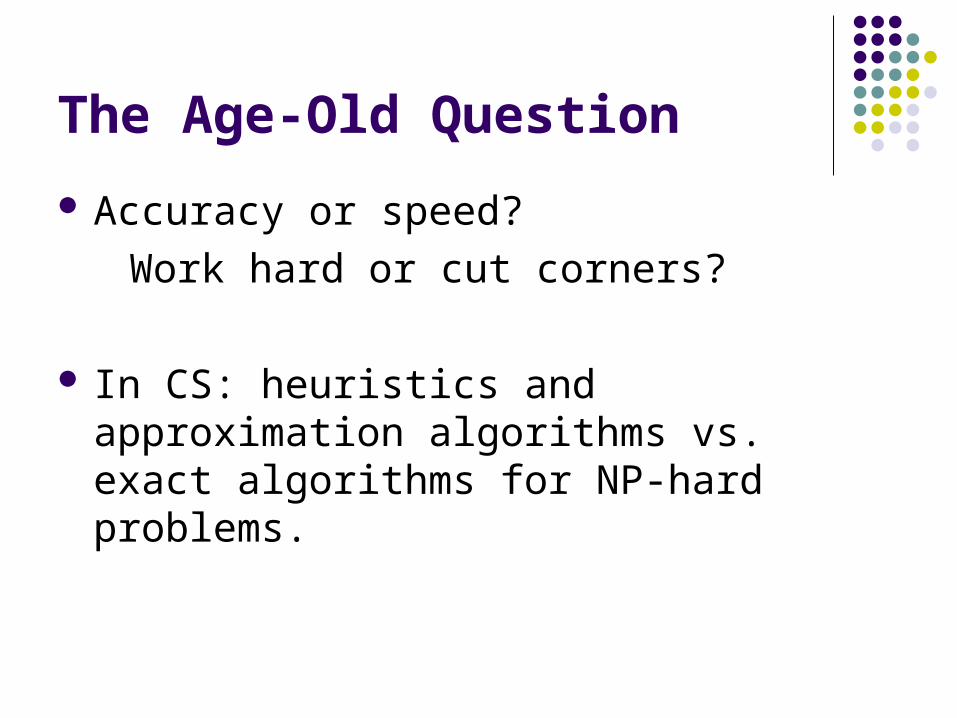
The Age-Old Question
Accuracy or speed?
Work hard or cut corners?
The Age-Old Question
Accuracy or speed?
Work hard or cut corners?
In CS: heuristics and approximation algorithms vs. exact algorithms for NP-hard problems.

The Age-Old Question
Both well-explored. But…
The Age-Old Question
Both well-explored. But…
“Constant time is the new polynomial time.”

The Age-Old Question
Both well-explored. But…
“Constant time is the new polynomial time.”
So, are there any corners left to cut?

The Setting
Given a set of n inputs x and a property P, determine if P(x) holds.

The Setting
Given a set of n inputs x and a property P, determine if P(x) holds.
Generally takes at least n steps (for sequential, nonadaptive algorithms).
The Setting
Given a set of n inputs x and a property P, determine if P(x) holds.
Generally takes at least n steps. (for sequential, nonadaptive algorithms).
Possibly infeasible if we are doing: internet or genome analysis, program checking, PCPs,…

First Compromise
What if we only want a check that rejects any x such that ~P(x), with probability > 2/3? Can we do better?
First Compromise
What if we only want a check that rejects any x such that ~P(x), with probability > 2/3? Can we do better?
Intuitively, we must expect to look at ‘almost all’ input bits if we hope to reject x that are only one bit away from satisfying P.

First Compromise
What if we only want a check that rejects any x such that ~P(x), with probability > 2/3? Can we do better?
Intuitively, we must expect to look at ‘almost all’ input bits if we hope to reject x that are only one bit away from satisfying P.
So, no.
Second Compromise
This kind of failure is universal. So, we must scale our hopes back.

Second Compromise
This kind of failure is universal. So, we must scale our hopes back.
The problem: those almost-correct instances are too hard.
Second Compromise
This kind of failure is universal. So, we must scale our hopes back.
The problem: those almost-correct instances are too hard.
The solution: assume they never occur!
Second Compromise
Only worry about instances y that either satisfy P or are at an ‘edit distance’ of c*n from any satisfying instance. (we say y is c-bad.)

Second Compromise
Only worry about instances y that either satisfy P or are at an ‘edit distance’ of c*n from any satisfying instance. (we say y is c-bad.)
Justifying this assumption is app-specific; the ‘excluded middle’ might not arise, or it might just be less important.
Model Decisions
Adaptive or non-adaptive queries?

Model Decisions
Adaptive or non-adaptive queries?
Adaptivity can be dispensed with at the cost of (exponentially many) more queries.

Model Decisions
Adaptive or non-adaptive queries?
Adaptivity can be dispensed with at the cost of (exponentially many) more queries.
One-sided or two-sided error?

Model Decisions
Adaptive or non-adaptive queries?
Adaptivity can be dispensed with at the cost of (exponentially many) more queries.
One-sided or two-sided error?
Error probability can be diminished by repeated trials.

The ‘Trivial Case’: Statistical Sampling
Let P(x) = 1 iff x is all-zeroes.
The ‘Trivial Case’: Statistical Sampling
Let P(x) = 1 iff x is all-zeroes.
Then y is c-bad, if and only if ||y|| >= c*n.

The ‘Trivial Case’: Statistical Sampling
Algorithm: sample O(1/c) random, independently chosen bits of y, accepting iff all bits come up 0.
The ‘Trivial Case’: Statistical Sampling
Algorithm: sample O(1/c) random, independently chosen bits of y, accepting iff all bits come up 0.
If y is c-bad, a 1 will appear with probability 2/3.

The ‘Trivial Case’: Statistical Sampling
Algorithm: sample O(1/c) random, independently chosen bits of y, accepting iff all bits come up 0.
If y is c-bad, a 1 will appear with probability 2/3.
Sort-Checking [EKKRV98]
Given a list L of n numbers, let P(L) be the property that L is in nondecreasing order. How to test for P with few queries?
(Now queries are to numbers, not bits.)

Sort-Checking [EKKRV98]
First try: Pick k random entries of L, check that their contents are in nondecreasing order.
Sort-Checking [EKKRV98]
First try: Pick k random entries of L, check that their contents are in nondecreasing order.
Correct on sorted lists…

Sort-Checking [EKKRV98]
First try: Pick k random entries of L, check that their contents are in nondecreasing order.
Correct on sorted lists…
Suppose L is c-bad; what k will suffice to reject L with probability 2/3?

Sort-Checking (cont’d)
Uh-oh, what about L = (2, 1, 4, 3, 6, 5, …, 2n, 2n - 1)?

Sort-Checking (cont’d)
Uh-oh, what about L = (2, 1, 4, 3, 6, 5, …, 2n, 2n - 1)?
It’s ½-bad, yet we need k ~ sqrt(n) to succeed.
Sort-Checking (cont’d)
Uh-oh, what about L = (2, 1, 4, 3, 6, 5, …, 2n, 2n - 1)?
It’s ½-bad, yet we need k ~ sqrt(n) to succeed.
Modify the algorithm to test adjacent pairs? But this algorithm, too, has its blind spots.

An O(1/c * log n) solution [EKKRV98]
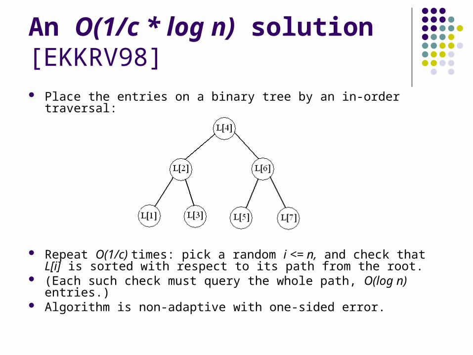
Place the entries on a binary tree by an in-order traversal:

An O(1/c * log n) solution [EKKRV98] Place the entries on a binary tree by an in-order traversal:
Repeat O(1/c) times: pick a random i <= n, and check that L[i] is sorted with respect to its path from the root.
An O(1/c * log n) solution [EKKRV98] Place the entries on a binary tree by an in-order traversal:
Repeat O(1/c) times: pick a random i <= n, and check that L[i] is sorted with respect to its path from the root.
(Each such check must query the whole path, O(log n) entries.) Algorithm is non-adaptive with one-sided error.
Sortchecking Analysis
If L is sorted, each check will succeed.
Sortchecking Analysis
If L is sorted, each check will succeed.
What if L is c-bad? Equivalently, what if L contains no nondecreasing subsequence of length (1-c)*n?

Sortchecking Analysis
It turns out that a contrapositive analysis works more easily.

Sortchecking Analysis
It turns out that a contrapositive analysis works more easily.
That is, suppose most such path-checks for L succeed; we argue that L must be close to a sorted list L’ which we will define.

Sortchecking Analysis (cont’d)
Let S be the set of indices for which the path-check succeeds.
Sortchecking Analysis (cont’d)
Let S be the set of indices for which the path-check succeeds.
If a path-check of a randomly chosen element succeeds with probability > (1 – c), then
|S| > (1 – c)*n.
Sortchecking Analysis (cont’d)
Let S be the set of indices for which the path-check succeeds.
If a path-check of a randomly chosen element succeeds with probability > (1 – c), then
|S| > (1 – c)*n. We claim that L, restricted to S, is in
nondecreasing order!

Sortchecking Analysis (cont’d)
Then, by ‘correcting’ entries not in S to agree with the order of S, we get a sorted list L’ at edit distance < c*n from L.

Sortchecking Analysis (cont’d)
Then, by ‘correcting’ entries not in S to agree with the order of S, we get a sorted list L’ at edit distance < c*n from L.
So L cannot be c-bad.

Sortchecking Analysis (cont’d)
Thus, if L is c-bad, it fails each path-check with probability > c, and O(1/c) path-checks expose it with probability 2/3.

Sortchecking Analysis (cont’d)
Thus, if L is c-bad, it fails each path-check with probability > c, and O(1/c) path-checks expose it with probability 2/3.
This proves correctness of the (non-adaptive, one-sided error) algorithm.
Sortchecking Analysis (cont’d)
Thus, if L is c-bad, it fails each path-check with probability > c, and O(1/c) path-checks expose it with probability 2/3.
This proves correctness of the (non-adaptive, one-sided error) algorithm.
[EKKRV98] also shows this is essentially optimal.
First Moral
We saw that it can take insight to discover and analyze the right ‘local signature’ for the global property of failing to satisfy P.

Second Moral
This, and many other property-testing algorithms, work because they implicitly define a correction mechanism for property P.
Second Moral
This, and many other property-testing algorithms, work because they implicitly define a correction mechanism for property P.
For an algebraic example:

Linearity Testing [BLR93]
Given: a function f: {0,1}^n {0, 1}.

Linearity Testing [BLR93]
Given: a function f: {0,1}^n {0, 1}.
We want to differentiate, probabilistically and in few queries, between the case where f is linear
(i.e., f(x+y)=f(x)+f(y) (mod 2) for all x, y),

Linearity Testing [BLR93]
Given: a function f: {0,1}^n {0, 1}.
We want to differentiate, probabilistically and in few queries, between the case where f is linear
(i.e., f(x+y)=f(x)+f(y) (mod 2) for all x, y),
and the case where f is c-far from any linear function.
Linearity Testing [BLR93]
How about the naïve test: pick x, y at random, and check that
f(x+y)=f(x)+f(y) (mod 2)?

Linearity Testing [BLR93]
How about the naïve test: pick x, y at random, and check that
f(x+y)=f(x)+f(y) (mod 2)?
Previous sorting example warns us not to assume this is effective…
Linearity Testing [BLR93]
How about the naïve test: pick x, y at random, and check that
f(x+y)=f(x)+f(y) (mod 2)?
Previous sorting example warns us not to assume this is effective…
Are there ‘pseudo-linear’ functions out there?

Linearity Test - Analysis
If f is linear, it always passes the test.

Linearity Test - Analysis
If f is linear, it always passes the test. Now suppose f passes the test with
probability > 1 – d, where d < 1/12;

Linearity Test - Analysis
If f is linear, it always passes the test. Now suppose f passes the test with
probability > 1 – d, where d < 1/12; we define a linear function g that is 2d-close
to f.

Linearity Test - Analysis
If f is linear, it always passes the test. Now suppose f passes the test with
probability > 1 – d, where d < 1/12; we define a linear function g that is 2d-close
to f. So, if f is 2d-bad, it fails the test with
probability > d, and O(1/d) iterations of the test suffice to reject f with probability 2/3.

Linearity Test - Analysis
Define g(x) = majority ( f(x+r)+f(r) ),
over a random choice of vector r.

Linearity Test - Analysis
Define g(x) = majority ( f(x+r)+f(r) ),
over a random choice of vector r.
f passes the test with probability at most
1 – t/2, where t is the fraction of entries where g and f differ.
Linearity Test - Analysis Define g(x) = majority ( f(x+r)+f(r) ), over a random choice of vector r.
f passes the test with probability at most 1 – t/2, where t is the fraction of entries where g and
f differ.
1 – t/2 > 1 – d implies t < 2d, so f, g are 2d-close, as claimed.

Linearity Test - Analysis
Now we must show g is linear.

Linearity Test - Analysis
Now we must show g is linear.
For c < 1, let G_(1-c) =
{x: with probability > 1-c over r,
f(x) = f(x+r)+f(r) }.
Let t_c = 1 - |G_(1-c)|/ 2^n.

Linearity Test - Analysis
Reasoning as before, we have t_c < d / c.
Linearity Test - Analysis
Reasoning as before, we have t_c < d / c.
Thus, t_(1/6) < 6d < 1/2.
Linearity Test - Analysis
Reasoning as before, we have t_c < d / c.
Thus, t_(1/6) < 6d < 1/2.
Then, given any x, there must exist a z such that z, x+z are both in G_5/6.
Linearity Test - Analysis
Now, what is Prob[g(x) = f(x+r) + f(r)]?
(How ‘resoundingly’ is the majority vote decided for an arbitrary x?)
Linearity Test - Analysis
Now, what is Prob[g(x) = f(x+r) + f(r)]?
(How ‘resoundingly’ is the majority vote decided for an arbitrary x?)
It’s the same as
Prob[g(x) = f(x + (z+r)) + f(z+r)],
Linearity Test - Analysis
Now, what is Prob[g(x) = f(x+r) + f(r)]? (How ‘resoundingly’ is the majority vote decided for
an arbitrary x?)
It’s the same as Prob[g(x) = f(x + (z+r)) + f(z+r)], since for fixed z, z+r is uniformly distributed if r
is.
Linearity Test - Analysis
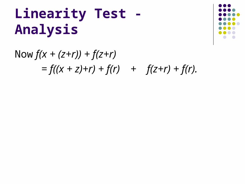
Now f(x + (z+r)) + f(z+r)
= f((x + z)+r) + f(r) + f(z+r) + f(r).

Linearity Test - Analysis
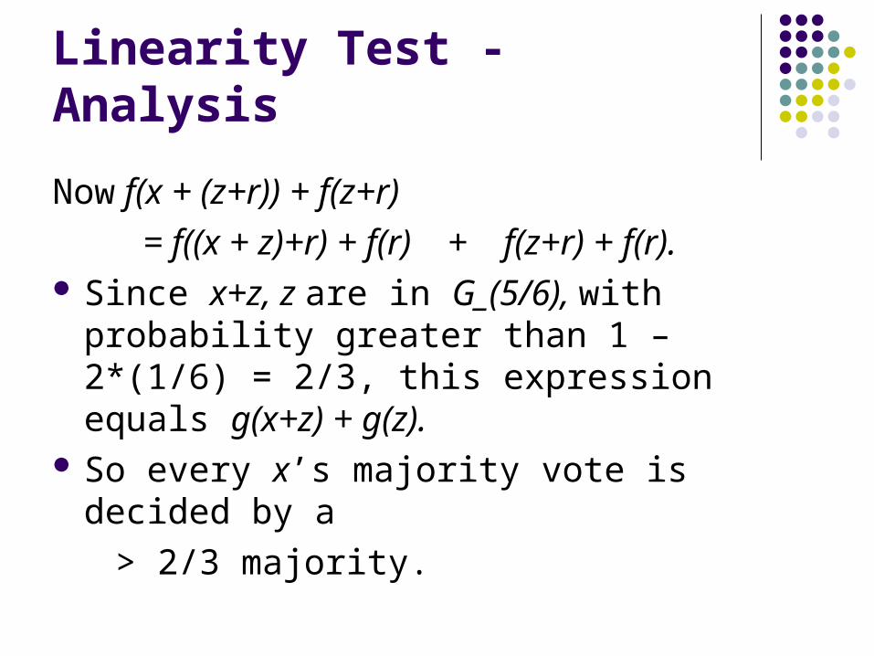
Now f(x + (z+r)) + f(z+r)
= f((x + z)+r) + f(r) + f(z+r) + f(r). Since x+z, z are in G_(5/6), with probability
greater than 1 – 2*(1/6) = 2/3, this expression equals g(x+z) + g(z).
Linearity Test - Analysis
Now f(x + (z+r)) + f(z+r)
= f((x + z)+r) + f(r) + f(z+r) + f(r). Since x+z, z are in G_(5/6), with probability
greater than 1 – 2*(1/6) = 2/3, this expression equals g(x+z) + g(z).
So every x’s majority vote is decided by a
> 2/3 majority.
Linearity Test - Analysis
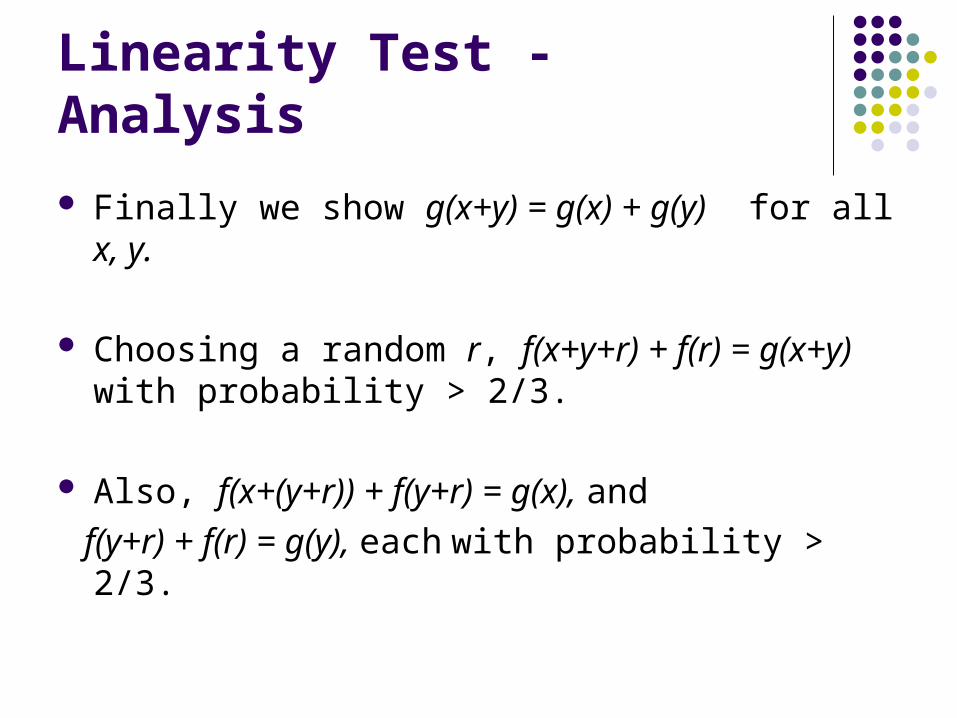
Finally we show g(x+y) = g(x) + g(y) for all x, y.

Linearity Test - Analysis
Finally we show g(x+y) = g(x) + g(y) for all x, y.
Choosing a random r, f(x+y+r) + f(r) = g(x+y) with probability > 2/3.
Linearity Test - Analysis
Finally we show g(x+y) = g(x) + g(y) for all x, y.
Choosing a random r, f(x+y+r) + f(r) = g(x+y) with probability > 2/3.
Also, f(x+(y+r)) + f(y+r) = g(x), and
f(y+r) + f(r) = g(y), each with probability > 2/3.
Linearity Test - Analysis
Finally we show g(x+y) = g(x) + g(y) for all x, y.
Choosing a random r, f(x+y+r) + f(r) = g(x+y) with probability > 2/3.
Also, f(x+(y+r)) + f(y+r) = g(x), and f(y+r) + f(r) = g(y), each with probability > 2/3.
Then with probability > 1 – 3 * (1/3) > 0, all 3 occur. Adding, we get g(x+y) = g(x) + g(y). QED.

Testing Graph Properties
A ‘graph property’ should be invariant under vertex permutations.
Testing Graph Properties
A ‘graph property’ should be invariant under vertex permutations.
Two query models: i) adjacency matrix queries, ii) neighborhood queries.
Testing Graph Properties
A ‘graph property’ should be invariant under vertex permutations.
Two query models: i) adjacency matrix queries, ii) neighborhood queries.
ii) appropriate for sparse graphs.
Testing Graph Properties
For hereditary graph properties, most common testing algorithms simply check random subgraphs for the property.

Testing Graph Properties
For hereditary graph properties, most common testing algorithms simply check random subgraphs for the property.
E.g., to test if a graph is triangle-free, check a small random subgraph for triangles.

Testing Graph Properties
For hereditary graph properties, most common testing algorithms simply check random subgraphs for the property.
E.g., to test if a graph is triangle-free, check a small random subgraph for triangles.
Obvious algorithms, but often require very sophisticated analysis.

Testing Graph Properties(Cont’d)
Efficiently testable properties in model i) include:

Testing Graph Properties(Cont’d)
Efficiently testable properties in model i) include: Bipartiteness
Testing Graph Properties(Cont’d)
Efficiently testable properties in model i) include: Bipartiteness 3-colorability

Testing Graph Properties(Cont’d)
Efficiently testable properties in model i) include: Bipartiteness 3-colorability In fact [AS05], every property that’s ‘monotone’ in
the entries of the adjacency matrix!

Testing Graph Properties(Cont’d)
Efficiently testable properties in model i) include: Bipartiteness 3-colorability In fact [AS05], every property that’s ‘monotone’ in
the entries of the adjacency matrix! A combinatorial characterization of the testable
graph properties is known [AFNS06].
Lower Bounds via Yao’s Principle
A q-query probabilistic algorithm A testing for property P can be viewed as a randomized choice among q-query deterministic algorithms {T[i]}.

Lower Bounds via Yao’s Principle
A q-query probabilistic algorithm A testing for property P can be viewed as a randomized choice among q-query deterministic algorithms {T[i]}.
We will look at the 2-sided error model.

Lower Bounds via Yao’s Principle
For any distribution D on inputs, the probability that A accepts its input is a weighted average of the acceptance probabilities of the {T[i]}.

Lower Bounds via Yao’s Principle
Suppose we can find (D_Y, D_N): two distributions on inputs, such that

Lower Bounds via Yao’s Principle
Suppose we can find (D_Y, D_N): two distributions on inputs, such that
i) x from D_Y all satisfy property P;

Lower Bounds via Yao’s Principle
Suppose we can find (D_Y, D_N): two distributions on inputs, such that
i) x from D_Y all satisfy property P; ii) x from D_N all are c-bad;

Lower Bounds via Yao’s Principle
Suppose we can find (D_Y, D_N): two distributions on inputs, such that
i) x from D_Y all satisfy property P; ii) x from D_N all are c-bad; iii) D_Y and D_N are statistically 1/3-close on
any fixed q entries.
Lower Bounds via Yao’s Principle
Then, given a non-adaptive deterministic q-query algorithm T[i], the statistical distance between T[i](D_Y) and T[i](D_N) is at most 1/3, so the same holds for our randomized algorithm A!

Lower Bounds via Yao’s Principle
Then, given a non-adaptive deterministic q-query algorithm T[i], the statistical distance between T[i](D_Y) and T[i](D_N) is at most 1/3, so the same holds for our randomized algorithm A!
Thus A cannot simultaneously accept all P-satisfying instances with prob. > 2/3 and accept all c-bad instances with prob. < 1/3.

Example: Graph Isomorphism
Let P(G_1, G_2) be the property that G_1 and G_2 are isomorphic.
Example: Graph Isomorphism
Let P(G_1, G_2) be the property that G_1 and G_2 are isomorphic.
Let D_Y be distributed as (G, pi(G)), where G is a ‘random graph’ and pi a random permutation;

Example: Graph Isomorphism
Let P(G_1, G_2) be the property that G_1 and G_2 are isomorphic.
Let D_Y be distributed as (G, pi(G)), where G is a ‘random graph’ and pi a random permutation;
Let D_N be distributed as (G_1, G_2), where G_1, G_2 are independent random graphs.
Example: Graph Isomorphism
Briefly: (G_1, G_2) is almost always far from satisfying P because for any fixed permutation pi, the adjacency matrices of G_1 and pi(G_2) are ‘too unlikely’ to be similar;

Example: Graph Isomorphism
Briefly: (G_1, G_2) is almost always far from satisfying P because for any fixed permutation pi, the adjacency matrices of G_1 and pi(G_2) are ‘too unlikely’ to be similar;
D_Y ‘looks like’ D_N as long as we don’t query both a lhs vertex of G and its rhs counterpart in pi(G)—and pi is unknown.
This approach proves a sqrt(n) query lower bound.

Concluding Thoughts
Property Testing: Revitalizes the study of familiar properties
Concluding Thoughts
Property Testing: Revitalizes the study of familiar properties Leads to simply stated, intuitive, yet
surprisingly tough conjectures

Concluding Thoughts
Property Testing: Contains ‘hidden layers’ of algorithmic
ingenuity

Concluding Thoughts
Property Testing: Contains ‘hidden layers’ of algorithmic
ingenuity Brilliantly meets its own lowered standards
Acknowledgments
Thanks for Listening!
Thanks to Russell Impagliazzo and Kirill Levchenko for their help.

References [AS05]. Alon, Shapira: Every Monotone Graph Property is
Testable, STOC ’05. [AFNS06]. Alon, Fischer, Newman, Shapira: A combinatorial
characterization of the testable graph properties: it's all about regularity, STOC ’06.
[BLR93] Manuel Blum, Michael Luby, and Ronitt Rubinfeld. Self-testing/correcting with applications to numerical problems. Journal of Computer and System Sciences, 47(3):549–595, 1993. (linearity test)
[EKKRV98]F. Erg¨un, S. Kannan, S. R. Kumar, R. Rubinfeld, and M. Viswanathan. Spot-checkers. STOC 1998. (sort-checking)
[F97] Eldar Fischer: The Art of Uninformed Decisions. Bulletin of the EATCS 75: 97 (2001) (survey on property testing)