Alexandra BystrÃ¶m Print III - DiVA...

DOCTORA L T H E S I S

Department of Civil, Environmental and Natural Resources EngineeringDivision of Structural and Fire Engineering Compartment Fire Temperature:

Calculations and Measurements

Alexandra Byström

ISSN 1402-1544ISBN 978-91-7583-812-0 (print)ISBN 978-91-7583-813-7 (pdf)

Luleå University of Technology 2017

Alexandra B

yström C

ompartm

ent Fire Temperature: C

alculations and Measurem

ents Steel Structures

Division of Structural and Fire EngineeringDepartment of Civil, Environmental and Natural Resources Engineering

Luleå University of Technology SE - 971 87 LULEÅ

www.ltu.se/sbn

DOCTORAL THESIS

COMPARTMENT FIRE TEMPERATURE: CALCULATIONS AND MEASUREMENTS

Alexandra Byström Luleå, 2017

Division of Structural and Fire Engineering Department of Civil, Environmental and Natural Resources Engineering

Luleå University of Technology SE - 971 87 LULEÅ

www.ltu.se/sbn

DOCTORAL THESIS

COMPARTMENT FIRE TEMPERATURE: CALCULATIONS AND MEASUREMENTS

Alexandra Byström

Luleå, March 2017

Printed by Luleå University of Technology, Graphic Production 2017

ISSN 1402-1544 ISBN 978-91-7583-812-0 (print)ISBN 978-91-7583-813-7 (pdf)

Luleå 2017

www.ltu.se

Abstract

I

Abstract

This thesis is devoted to heat transfer and fire dynamics in enclosures. It consists of a main part which summarizes and discusses the theory of heat transfer, conservation of energy, fire dynamics and specific fire scenarios that have been studied. In the second part of this thesis, the reader will find an Appendix containing seven scientific publications in this field.

In particular, one- and two-zone compartment fire models have been studied. A new way of calculating fire temperatures of pre- and post-flashover compartment fires is presented. Three levels of solution techniques are presented including closed form analytical expressions, spread-sheet calculations and solutions involving general finite element temperature calculations. Validations with experiments have shown good accuracy of the calculation models and that the thermal properties of the surrounding structures have a great impact on the fire temperature development. In addition, the importance of the choice of measurement techniques in fire engineering has been studied. Based on the conclusions from these studies, the best techniques have been used in further experimental studies of different fire scenarios.

Keywords: compartment fire temperature, heat transfer, FEM, calculation of temperature, temperature measurement, fire scenario, validation, flashover.

Abstract in Swedish

III

Abstract in Swedish

Denna avhandling behandlar problem kopplade till värmeöverföring och branddynamik i slutna utrymmen med tonvikt på värmeöverföring mellan gaser och utsatta konstruktioner. Avhandlingen består av en huvuddel och ett appendix innehållande sju vetenskapliga artiklar. I huvuddelen sammanfattas och diskuteras grundläggande teorier och principer inom värmeöverföring och branddynamik samt studier av ett antal specialfall av brandscenarion som baseras på dessa teorier. I de avslutande bilagorna (Artiklar A1-A3 och Artiklar B1-B2) finns sju vetenskapliga artiklar som grundligare beskriver de ovan nämnda specialfallen.

Huvudfokus i avhandlingen ligger på temperaturutveckling vid brand i slutna utrymmen. I avhandlingen studeras i synnerhet en- och två-zonsmodeller för brand i slutna utrymmen, och en ny metod för att beräkna brandgastemperaturer före och efter övertändning i rumsbränder är framtagen. Validering av dessa modeller med experiment visar att deras noggrannhet är bra. Modellerna visar också att de termiska egenskaperna hos de omgivande ytorna har stor inverkan på brandtemperatursutvecklingen. I tillägg studeras i denna avhandling betydelsen av val av mätmetoder i brandtekniska tillämpningar. På grundval av slutsatserna från dessa studier har de främsta mätteknikerna använts i ytterligare experimentella studier av olika brandscenarier.

Nyckelord: brandtemperaturer i slutna utrymmen, värmeöverföring, FEM, temperaturberäkning, temperaturmätning, brandmodellering, validering, övertändning.

Contents

V

Contents

ABSTRACT ......................................................................................................... I

ABSTRACT IN SWEDISH .............................................................................. III

CONTENTS ....................................................................................................... V

ACKNOWLEDGMENT ................................................................................... IX

ABBREVIATIONS .......................................................................................... XI

1 INTRODUCTION ..................................................................................... 1 1.1 Literature review .............................................................................. 3 1.2 Objectives and research questions ................................................... 5 1.3 Limitations ....................................................................................... 6 1.4 Scientific approach ........................................................................... 6 1.5 Structure of the thesis ....................................................................... 7 1.6 Short summaries of appended papers ............................................... 8 1.7 Additional work (not included in this thesis) ................................. 10

2 THEORETICAL BACKGROUND ........................................................ 13 2.1 Heat transfer ................................................................................... 13

2.1.1 Radiation ............................................................................ 14 2.1.2 Convection .......................................................................... 15 2.1.3 Boundary conditions ........................................................... 16 2.1.4 Unsteady-state conduction ................................................. 18 2.1.5 Heat transfer in fire safety engineering .............................. 19

2.2 Fire dynamics ................................................................................. 23 2.2.1 Conservation of mass ......................................................... 23 2.2.2 Conservation of energy ...................................................... 25

Compartment fire temperature: calculations and measurements

VI

3 METHODS .............................................................................................. 31 3.1 Literature review ............................................................................ 31 3.2 Experimental studies ...................................................................... 32

3.2.1 Experiments in laboratory facilities ................................... 32 3.2.2 Experiments in the field ..................................................... 36

3.3 Computation models for compartment fire .................................... 39 3.4 Numerical modelling ..................................................................... 39 3.5 Influence of various parameters ..................................................... 41

4 MEASURING TECHNIQUES ............................................................... 43 4.1 Thermocouple ................................................................................ 44 4.2 Heat flux meter, HFM .................................................................... 45 4.3 Plate thermometer .......................................................................... 46

4.3.1 Alternatively designed Plate Thermometers ...................... 46 4.3.2 Corrections of PT measurements ....................................... 49

5 COMPARTMENT FIRE MODELS ....................................................... 53 5.1 Limitations ..................................................................................... 54 5.2 Compartment fire models .............................................................. 54 5.3 Analogous electrical model ............................................................ 55

5.3.1 General formulation of the new fire models ...................... 56 5.3.2 Heat transfer at the surface of the surroundings................. 59

5.4 New calculation models ................................................................. 60 5.4.1 Analytical solution ............................................................. 60 5.4.2 Numerical solutions ........................................................... 61

5.5 Validation of the models ................................................................ 63

6 DISCUSSIONS AND CONCLUSIONS ................................................. 65 6.1 Addressing the research questions ................................................. 65 6.2 Future research ............................................................................... 70

REFERENCES ................................................................................................. 71

PAPERS A ............................................................................................................ Paper A1 ...................................................................................................... Paper A2 ...................................................................................................... Paper A3 ......................................................................................................

PAPERS B ............................................................................................................ Paper B1 ...................................................................................................... Paper B2 ...................................................................................................... Paper B3 ...................................................................................................... Paper B4 ......................................................................................................

Acknowledgment

VII

Acknowledgment

The research work presented in this thesis was carried out at the Department of Civil, Environmental and Natural Resources at Luleå University of Technology (LTU), in the Research Group of Steel Structures at the Division of Structural and Fire Engineering.

I gratefully acknowledge the financial support provided by The Swedish fire research board, Brandforsk, Sweden, as well as that provided by Europeiska regionala utvecklingsfonden, En investering för framtiden, project NSS, Nordic Safety and Security, 2008-2011. I would also like to acknowledge the support by Wallenbergstiftelsen – Jubileumsanslaget, for giving me a possibility to meet other researchers in my field during conferences in Switzerland and Portugal.

I would like to sincerely thank my supervisor, Professor Ulf Wickström, who has been an endless resource of knowledge, inspiration, support and who has guided me through every issue of heat transfer. Your research and personality is pure inspiration. I am grateful to know you.

I also would like to thank my co-supervisor Professor Michael Försth for valuable comments. He has been an incredibly valuable source of knowledge and inspiration for me since he joined LTU.

I am very grateful to Professor Milan Veljkovic who gave me this great opportunity to become a PhD student and to be part of interesting research projects in the beginning of my journey.

My sincere thanks also to my ex-colleague and co-author of some of my papers, associate Professor Xudong Cheng at University of Science & Technology of China, Hefei, for his indispensable collaboration and letting me gain from his knowledge and experience.


VIII

Many thanks also goes to the co-author of some of my papers, scientist and PhD Johan Sjöström at Technical Research Institute of Sweden, SP, Fire technology, for great collaboration, positivity, inspiration and just great ideas and solutions. It has been a pleasure working with you and I would be pleased to continue this collaboration in the future.

I would like to thank COMPLAB, the testing laboratory at the Department of Civil, Mining and Natural Resources Engineering, LTU for their help and cooperation.

A big thank you to the Luleå Emergency Training Center (Luleå Räddningstjänst utbildningscentrum), Hertsön, for letting us to use their facility for research purpose.

I am thankful for the assistance of the staff of Laboratory facility at Technical Research Institute of Sweden, SP, Fire technology for their valuable assistance carrying out fire tests.

I would also like to thank all my colleagues for making me feel part of the group, for all support and distraction.

What would it be without the greatest support of the families: some are so close in my heart but so far away from me in distance: my sisters and my mother who always believed in me even when I did not and my father who would have been so proud of me, my second family for welcoming me, supporting and being my extended family in Sweden. Last but not least, I would like to thank my family and especially my dear husband Johan for his love, support, encouragement, great help with my research spirit and my wonderful, full of love and energy children Alexander, Christian and William. All of this is meaningless without you.

Luleå, January 2017

Alexandra Byström

Abbreviations

IX

Abbreviations

Roman letters

A Area [m2]

Ao Area of openings [m2]

Atot Total surrounding area of enclosure [m2]

C Heat capacity coefficient [J/m2K]

c Specific heat capacity [J/(kg K)]

Cd Flow coefficient [-]

cp Specific heat at constant pressure [J/(kg K)]

ho Height of the openings [m2]

h Heat transfer coefficient [W/m2K]

ch Convection heat transfer coefficient [W/m2K]

rh Radiation heat transfer coefficient [W/m2K]

K Heat conduction coefficient [W/m2K]

k Thermal conductivity [W/(m K)]


X

m Mass [kg]

am Mass flow rate through the opening [kg/s]

im Mass flow rate in compartment [kg/s]

om Mass flow rate out [kg/s]

pm Plume mass flow rate [kg/s]

O Opening factor [m1/2]

P Pressure [Pa=N/m2]

q Heat flux [W/m2]

cq Heat release rate by combustion [W]

lq Heat loss rate by the flow of hot gases out of compartment openings [W]

rq Heat radiation out through the openings [W]

wq Losses to the surrounding structure [W]

R Thermal resistance [(m2 K)/W]

T Temperature [ºC or K]

gT Gas temperature [ºC or K]

rT Radiation temperature [ºC or K]

sT Surface temperature [ºC or K]

t Time [s]

v Velocity [m/s]

Abbreviations

XI

z Effective height of the plume above the burning area [m]

Greek letters

1 Flow constant [kg/(s·m5/2) ]

2 Constant describing the combustion energy developed per unit mass of air [(W·s)/kg ]

3 Correlation factor [kg/(m5/3·W1/3·s]

cH Complete heat of combustion [J/kg ]

Temperature increase [ºC or K]

Emissivity [-]

Density [kg/m3]

Stefan-Boltzmann constant [W/(m2K4)]

Time constant [s]

Configuration or shape factor [-]

Combustion efficiency [-]

Subscripts

abs Absorptivity

AST Adiabatic Surface Temperature

con Convection

emi Emitted

f Fire

F.C Fuel Controlled


XII

fl Flame

hfm Heat Flux Meter

g Gas

F.O Flashover

i Initial

inc Incident

PT Plate Thermometer

rad Radiation

ref Reflectivity

s Surface

TC Thermocouple

tot Total

trans Transmissivity

ult Ultimate

V.C Ventilation Controlled

Ambient

Introduction

1

1 INTRODUCTION

Fire development in enclosures goes through the following phases: ignition, fire growth and eventually a fire may grow to a fully developed fire when flashover is reached (Walton & Thomas 2002), followed by a cooling phase.

During the ignition and growth phases, the main concern is lifesaving (Harmathy & Mehaffey 1983). The temperatures in the compartment are then generally moderate and not a threat to structures. The fire is limited to the amount of available pyrolysed gaseous fuel and can be defined as a fuel-controlled or pre-flashover fire. If a flashover is reached, a fully developed fire occurs. Fire burns at its maximum potential of the available air supply and can be defined as a ventilation-controlled or post-flashover fire. At the fully developed stage, temperatures rise considerably and may be a threat to the performance of the loadbearing structures. It is therefore in general this stage of a fire which is considered in the design of structural fire resistance. The main concern in this thesis is the stage when a developed compartment fire might affect the stability of structures.

According to Hurley and Rosenbaum (Hurley & Rosenbaum 2015), performance based design of structural fire resistance can be done using the following approach:

1) Determine the fire exposure to which a structure could be subjected.

2) Determine the thermal response of the structure. It involves heat transfer analysis based on the determined fire temperature.

3) Predict the mechanical performance of structural members and of the total building structure.


2

Usually structures are designed to resist the standard fire according to ISO 834 (ISO834-1 1999) or EN 1363-1 (EN1363-1 2012) for a specified time. Alternatively, parametric fires as specified in Eurocode 1, Annex A (EN1991-1-2 2002) could be applied for compartments less than 500 m2. In larger spaces, possible intense local fire exposure must also be considered.

During the past 10-20 years, much work has gone into development of advanced fire models. Development in information technology has contributed to reduction of calculation times and user interfaces have become friendlier, which has made advanced models commonly used. The number of numerical models identified by the fire engineering community has been increasing essentially the last 25 years.

However, more sophisticated models require good knowledge and understanding of fire phenomena. Such models are often computationally expensive, i.e. require extensive computer times and can sometimes produce erroneous results due to numerical instabilities. It is always recommended that numerical results are validated with experiments (if possible). Sometimes simpler methods can be used to assure the right order of magnitude.

Validation is aimed at different levels of complexity and therefore different types of experimental data are needed. The difference between a model’s prediction and an experiment’s measurement is a combination of three main components according to NUREG-1824 (U.S.NRC 2014):

- uncertainty in the measurement of the predicted quantity, related uncertainties in measured input, e.g. the experimental uncertainties reported in NUREG/CR-6905 (Hamins et al. 2006).

- uncertainty in the model input parameters.

- uncertainty in the model physics and numerics.

The accuracy of temperature measurements is very important for validation of mathematical fire models. Moreover, for performance based design it is important to be able to predict and estimate the right temperature to which construction elements can be exposed. In addition, there are large differences in the fire exposure to structures. The differences lie both in where and how the temperatures are probed but mostly in what type of material the wall is made of.

Introduction

3

In the case of a fire resistance test, usually thermocouples are used. However, a temperature measured by thermocouples may significantly differ from the true gas temperature due to the effect of radiation from flames, smoke layers, heated surroundings (Pitts et al. 1998; Blevins 1999; Blevins & Pitts 1999), soot effects, emissivity uncertainties or convection heat transfer correlations (Whitaker 1972). Measured temperatures depend on how they are probed, e.g. using plate thermometers (PTs) or thermocouples (TCs) (Sjöström et al. 2016). So called plate thermometers measure approximately the adiabatic surface temperature (AST), which is a suitable quantity when calculating heat transfer from fires to structures. The Plate Thermometer was invented to measure and control temperature in fire resistance furnaces (Wickström 1994).

Several researchers have studied compartment fires experimentally and several models have been published on estimating post-flashover compartment fire development, see e.g. (SFPE 2004; Walton & Thomas 2002).

The work presented in this thesis has been focused on the development of novel mathematical formulations of models for computing temperature of post- and pre-flashover fires in a single room compartment. Like other similar models, see (SFPE 2004; Walton & Thomas 2002), the models described in this thesis are based on an analysis of the energy and mass balance within a single fire compartment. However, the mathematical solution techniques in this model have been altered in such a way that it can be used to calculate fire temperatures in compartments with various types of surrounding structures. Several new parameters have been identified which facilitates the overall understanding of the thermal dynamics of compartment fires.

1.1 Literature review

A large number of studies in enclosure fire have been carried out through the last decades. Starting from the early research conducted by Ingberg (Ingberg 1928), researchers have studied compartment fires. In 1958 Kawagoe (Kawagoe 1958) published a large number of fully developed fire experiments conducted in reduced scale concrete enclosures. Wood was used as a fuel. Several measurements were made, including temperature- and pressure-gradient within the enclosure, gas velocity, radiation and other parameters. The results confirmed that the temperature in an enclosure can be assumed uniform and that the air flow into the compartment depends on the geometry of the openings and enclosure. In a later work by some Japanese researchers the first energy balance expression for a fully developed compartment fire was published (Kawagoe & Sekine 1963). Ödeen in 1968 (Ödeen 1968) described a


4

series of experiments carried out in a concrete tunnel building. In the 1970s, Magnusson and Thelandersson (Magnusson & Thelandersson 1970) calculated fire compartment gas temperature-time curves based on heat and mass balance analyses. Their model input data consisted of fire load density, geometry of ventilations and thermal characteristics of the compartment (floor, walls and ceiling). The Magnusson & Thelandersson model (Magnusson & Thelandersson 1970) is known as the Swedish opening factor method. Later, in 1974, Magnusson and Thelandersson presented further results (Magnusson & Thelandersson 1974) in form of gas temperature-time curves of a complete process of fire for a range of opening factors and fuel loads.

Based on the work of Magnusson and Thelandersson (Magnusson & Thelandersson 1970), Wickström (Wickström 1985) proposed a modified way of expressing fully developed design fires based on the standard ISO 834 curve (ISO834-1 1999). This has later been adapted in EN 1991-1-2 (EN1991-1-2 2002). Later on, Franssen (Franssen 2000) and Feasey and Buchanan (Feasey & Buchanan 2002) have suggested modifications. Franssen (Franssen 2000) suggested new modifications that took into account multi layered walls for controlled fires. These modifications concern the equivalent thermal properties of multi material walls, the introduction of a minimum duration of the fire and the ventilation effect in case of fuel controlled fires. In 2002, Feasey and Buchanan (Feasey & Buchanan 2002) suggested a more accurate way to modify the dependence of the decay rate on the ventilation factor and thermal insulation.

Babrauskas developed a computer program for calculating post-flashover fire temperatures, COMPF2, (Babrauskas 1979) and used it to derived closed-form algebraic equations to estimate temperature development in post flashover compartment fires (Babrauskas 1981). A comprehensive review of existing correlation models can be found in the SFPE Engineering Guide to Fire Exposures to Structural Elements (SFPE 2004). Hurley (Hurley 2005) evaluated the temperature and burning rate predictions of several models that were presented in (SFPE 2004) to fully developed post-flashover compartment fires, the so called CIB experiments. These experiments were part of a large CIB (Conseil Internationale du Bâtiment) collaboration where a number of experiments were conducted in a variety of enclosures (Thomas & Heselden 1970; Thomas & Heselden 1972). These experiments were conducted in enclosures of reduced size and most of the test room models were constructed of only 10 mm thick asbestos millboard. Hurley’s conclusion was that most of these models overestimate the fire temperature. A similar analysis has been done by Hunt and Cutonilli (Hunt et al. 2010).

Introduction

5

A series of eight full-scale fire tests (Lennon & Moore 2003; Dowling & Moore 2004) were conducted in a compartment with overall dimensions of 12 m x 12 m. These experiments were part of a research project by Building Research Establishment (BRE) and are known as the Cardington fire tests. The tests were used for validation of Eurocode 1 (EN1991-1-2 2002) but some changes in assumption have later been considered in the analysis (Lennon & Moore 2003).

Since the middle of the 20th century, several researchers have been trying to define suitable criteria for flashover. Waterman in 1968 (Waterman 1968) conducted some experimental studies in a compartment 3.64 m by 3.64 m and 2.43 m high. He claimed that a heat flux of about 20 kW/m2 at the floor level was required for flashover to occur. Another conclusion was that the temperature just below the ceiling reached 600ºC (Waterman 1968). Since then, several models have been published to predict flashover (McCaffrey et al. 1981; Thomas 1981; Babrauskas 1980).

Models to predict the temperature of the hot gases in fuel-controlled or pre-flashover compartment fires are usually based on the amount and type of combustible fuel. The McCaffrey, Quintiere and Harkleroad model, known as the MQH model (McCaffrey et al. 1981), was derived based on comparisons with tests and assumptions of heat losses to surrounding structures depending on their thermal properties. Their model is empirical. Evegren and Wickström (Evegren & Wickström 2015) have published a new numerical model for estimating temperatures in pre-flashover fires where the fire enclosure boundaries are assumed to have lumped heat capacity. Their model is applicable for structures of steel sheets, with or without insulation, where the heat capacity of the insulation may be ignored.

1.2 Objectives and research questions

The main objectives of this thesis are to contribute to the fire safety science with:

- methods for measuring thermal exposure of fire exposed structures that can be measured in a simple and robust way.

- methods for predicting effective fire temperatures in enclosures for expressing thermal exposure of structures.

The following key research questions are addressed in this thesis:


6

1. How can thermal exposure of a structure be measured in a simple and robust way?

2. How can compartment fire temperature and thermal exposure be calculated, using simple and more advanced methods?

3. Which parameters determine compartment maximum fire temperature and temperature rise rate, respectively?

1.3 Limitations

The fire models described in this thesis are simplified models that focus on temperature calculation of fire exposed structures in single room enclosures with natural ventilation conditions. These models are limited to simple room configurations, but extensions can be made to other applications, such as tunnel-, mine- and underground fires. Fire spreading between compartments will also not be addressed in this thesis.

Moreover, this thesis is not focused on issues such as smoke development, smoke spread, evacuation etc. and does not include any guidance for overall fire safety design or risk assessment process.

1.4 Scientific approach

The work presented in this thesis is divided into two main parts: measuring techniques and compartment fire models. The first part is based on understanding of the heat transfer phenomena when a body is exposed to fire. This has been done in parallel with a series of experiments, both under laboratory and field conditions. The theory using the concept of adiabatic surface temperature (AST) as a boundary condition for heat transfer analysis of structures exposed to fire has been validated with experiments.

The second part is based on the understanding of temperature development in single room compartment fires. These models were formulated from analyses of heat and mass balance equations and are validated with a well-controlled series of experiments rather than correlations with experiments. The choice of measuring equipment was based on observations and conclusions from the first studies presented in this work.

The work presented in this thesis is based on these four main scientific methods, see Figure 1-1:

Introduction

7

1. Observation (of experiments) and understanding of the phenomenon of compartment fire. The understanding of this phenomenon has been achieved by literature studies on the theories of heat transfer and fire dynamics.

2. Formulation of a hypothesis/model to explain the phenomenon of compartment fire in the form of a mathematical and physical relation.

3. Validation of a hypothesis/model with a series of well-controlled experiments. Study the effect of different parameters.

4. Formulate a final model/method and recommendations based on repeated verification of the results.

Figure 1-1. Scientific method.

1.5 Structure of the thesis

Chapter 2 summarizes the key theory of fire dynamics. Heat transfer in compartment fires is discussed in this part.

Chapter 3 focuses on the research methods that have been used to accomplish the work presented in this thesis.

Chapter 4 contains an overview of different thermal devices used to measure thermal exposure and the theory on how these measurements can be used. The main focus has been to study the use of the concept of adiabatic surface temperature (AST) in the compartment fire experiments.


8

Chapter 5 focuses on the development of novel mathematical formulation of models for computing temperature of post- and pre-flashover compartment fires. Model formulation, applicability and validation with experiments are overviewed in this chapter.

Chapter 6 discusses results and the main conclusions of the research work described in the previous chapters. Research questions are discussed and answered. Recommendations for future work are given.

Appendices, Papers A and Papers B, contain scientific articles on measuring techniques and compartment fire models, respectively. The appendices consist of five journal papers: three published in international research journals, one accepted and one submitted. In addition, there are two papers published in conference proceedings (Paper A1 was also published in a journal).

1.6 Short summaries of appended papers

A - Measuring techniques:

A1: “Use of plate thermometer for better estimate of fire development” by Alexandra Byström, Ulf Wickström, Milan Veljkovic. Published in 2011 in the Proceedings of the 3rd International workshop on Performance, Protection & Strengthening of Structures under Extreme Loading and in the Journal of Applied Mechanics and Materials, 82, pp. 362-367

This paper focuses on the use of the concept of adiabatic surface temperature (AST) together with Plate Thermometer (PT) measurements. Temperatures measured by PT were compared to the gas temperature measured by ordinary thermocouples (TCs), Ø=0.25 mm, and shielded thermocouples, Ø=3 mm. An experimental study was conducted in laboratory environment, using a cone calorimeter test (ISO5660-1 2002) under constant incident radiation exposure.

A2: “Measurement and calculation of adiabatic surface temperature in a full-scale compartment fire experiment” by Alexandra Byström, Xudong Cheng, Ulf Wickström, Milan Veljkovic. Published in 2012 in Journal of Fire Science, 31, 1, pp. 35-50.

This paper summarizes a fire experiment study in a two-story concrete building connected with a stairwell, during very low ambient temperature in Luleå, Sweden. The fuel was wood. Gas temperatures and temperatures measured by plate thermometers inside the compartment are presented.

Introduction

9

A3: “Large scale test on a steel column exposed to localized fire” by Alexandra Byström, Johan Sjöström, Ulf Wickström, David Lange, Milan Veljkovic. Published in Journal of Structural Fire Engineering, 2014, vol. 5, no 2, pp. 147-160.

This paper presents a full scale test of the exposure from localized fire on a steel column. Temperatures were measured by plate thermometers. Steel temperatures were calculated with the finite element method based on the gas temperature measurements and compared with measured steel temperatures. Comparisons were also made with estimates based on Eurocode 1 (EN1991-1-2 2002).

B – Compartment fire models:

B1: “Thermal analysis of a pool fire test in a steel container” by Xudong Cheng, Alexandra Byström, Ulf Wickström, Milan Veljkovic. Published in 2012 in Journal of Fire Sciences, Vol. 30 (2), pp. 170-184.

This paper presents results of a pool fire test conducted in a non-insulated steel container under low ambient temperature. During this experiment, temperatures were measured, analyzed and compared with numerically calculated temperatures by FDS.

B2: "Compartment fire temperature – a new simple calculation method” by Ulf Wickström, Alexandra Byström. Published in 2014 in Proceedings of 11th International Symposium on Fire Safety Science, University of Canterbury, New Zealand, February 10 – 14, 2014, pp. 289-301.

A new simplified method to calculate the ultimate fire temperature that can be reached in fully developed compartment fire is described. The theory and assumptions follow broadly the work of Magnusson and Thelandersson (Magnusson & Thelandersson 1970) and Pettersson et al (Pettersson et al. 1976). It has later been modified and reformulated by Wickström (Wickström 1985) and is the basis for the so called parametric fire curves in Eurocode 1, EN 1991-1-2, Annex A (EN1991-1-2 2002).

B3: "Temperature of post-flashover compartment fires – calculations and validation” by Alexandra Byström, Ulf Wickström. Accepted and to appear in Journal of Fire and Materials, 2017.

This paper describes and validates a one-zone fire model with a series of fully developed compartment fire tests conducted in a reduced scale compartment


10

(Sjöström et al. 2016). The model is based on an analysis of the energy and mass balance assuming combustion being limited by the availability of oxygen and is described in Paper B2. However, the mathematical solution techniques in this model have been altered which makes it possible to use a general finite element temperature calculation program for predicting compartment fire temperatures. Then combinations of materials and non-linearities such as material properties varying with temperature and moisture content can be considered.

B4: "Pre-flashover compartment fire temperature: a new calculation model validated with experiments” by Alexandra Byström, Ulf Wickström. Submitted to Fire Safety Journal, 2017.

This paper describes a two-zone model for computing temperature of pre-flashover compartment fires and validates it by comparisons with tests conducted in a reduced scale compartment (Sjöström et al. 2016). The model is based on an analysis of the energy balance and plume flow rate. The model takes into account the basic physics of heat transfer and thermodynamics.

1.7 Additional work (not included in this thesis)

In addition to the articles appended to this thesis, the following publications have also been achieved during the Ph.D. study period.

Journal papers

Byström A., Cheng X., Wickström U. & Veljkovic M. (2011). Full-scale experimental and numerical studies on compartment fire under low ambient temperature, Building and Environment, Vol. 51 (May 2012), 255-262.

Conference papers

Byström A., Sjöström J., Wickström U. (2016). Temperature measurements and modelling of flashed over compartment fires. In Proceedings of the 14th International Conference and Exhibition on fire science and engineering, Interflam , July 2016, Nr Windsor.

Introduction

11

Byström A., Wickström U. (2015). Influence of surrounding boundaries on fire compartment temperature. In Proceedings of Applications of Structural Fire Engineering, 15-16 October 2015, Dubrovnik, Croatia

Byström A., Lind O., Palmklint E., Jönsson P., Wickström U. (2015). Analysis of a new plate thermometer – the copper disc plate thermometer, In Proceedings of 1st International Fire Safety Symposium, IFireSS, 20th – 23rd April 2015, Coimbra, Portugal, 453-460.

Wickström U., Sjöström J. & Byström A. (2013). New method for calculating time to reach ignition temperature. In Proceedings of 13th International Conference and Exhibition on fire science and engineering, Interflam, June 2013, Nr Windsor, 735-742.

Wickström U., Byström A., Sandström J. & Veljkovic M. (2013). Reducing design steel temperature by accurate temperature calculations. In Proceedings of International conference Applications of structural fire engineering, April 2013, 290-298.

Byström A., Sjöström J., Wickström U. & Veljkovic M. (2012). A steel column exposed to localized fire. In Proceedings of the Nordic Steel Construction Conference, September 2012, Oslo, Norway, 401-410.

Byström A., Sjöström J., Wickström U. & Veljkovic M. (2012). Large scale test to explore thermal exposure of column exposed to localized fire. In Proceedings of 7th International Conference in Fire, SiF, June 2012, Zurich, Switzerland, 185- 194.

Cheng X., Veljkovic M., Byström A., Iqbal N., Sandström J. & Wickström U. (2011). Prediction of temperature variation in an experimental building. In Proceedings of International conference Applications of structural fire engineering, Protect, April 2011, Lugano, Switzerland, 387-392.

Technical reports

Sjöström, J., Wickström, U., Byström, A.(2016). Validation data for room fire models: Experimental background. Technical report, Project 307-131, SP Technical research Institute of Sweden, 2016


12

Byström, A., Sjöström, J., Wickström, U. (2016). Validation of a one-zone room fire modal with well-defined experiments. Technical report, Project 307-131, Luleå University of Technology, Financed by Brandforsk, Sweden 2016

Sjöström J., Byström A., Lange D. & Wickström U. (2012). Thermal exposure to a steel column from localized fires. Technical report 302-111, ISSN 0284-5172, SP Technical research Institute of Sweden.

Licentiate thesis

Byström A. (2013). Fire temperature development in enclosures: Some theoretical and experimental studies. Licentiate Thesis, Luleå University of Technology, Luleå; Sweden.

Theoretical background

13

2 THEORETICAL BACKGROUND

A compartment fire may be characterized by several phases: it starts from ignition and then moves into a growth stage. If no action is taken to suppress the fire and there is enough fuel, it may eventually grow to a maximum intensity fire that is controlled by the amount of air available through ventilation openings. When the fuel is consumed, the fire temperature will decrease.

This chapter describes the background of heat transfer and temperature calculation analyses of compartment fires.

2.1 Heat transfer

Heat can be transferred by three different mechanisms: conduction, convection and radiation. Conduction is the transfer of energy from more energetic particles (higher temperature) of a solid to less energetic ones as a result of interaction between particles. Convection is the transfer of energy between a solid surface and an adjacent fluid that is in motion. Radiation is the transfer of energy due to emission of electromagnetic waves.

The governing differential equation for two-dimensional heat conduction assuming a constant thermal conductivity k is:

2 2

2 2

T T c Tx y k t

(2.1)


14

The heat transfer from the flame and hot gases to a surface consists of three main independent components: absorbed radiative heat from the black body, emitted heat and heat transferred by convection, see Figure 2-1.

Figure 2-1. Heat transfer mechanism by radiation and convection at the

surface.

Thus:

'' '' '' ''tot abs emi conq q q q (2.2)

2.1.1 Radiation

When radiant energy meets a material surface, part of the energy will be reflected, part of it absorbed and part of it transmitted as shown in Figure 2-1. This can be written as:

1ref abs trans (2.3)

where ref is reflectivity – the fraction that is reflected, abs is absorptivity – the fraction that is absorbed and trans is transmissivity – the fraction that is transmitted. Most solid bodies do not transmit thermal radiation (Holman 2009). Hence the equation above can be written as:

1ref abs (2.4)

Surface absorptivity abs and surface emissivity s depend on the temperature and the wavelength of the radiation. As can be found in the literature (Holman 2009; Cengel 2008), according to Kirchhoff’s identity the emissivity and the absorptivity of a surface at a given temperature and a fixed wavelength are equal. In practical applications, the average absorptivity of a surface is taken to be equal to its average emissivity.


15

The absorbed radiation heat ''absq is proportional to the incident radiation and the

absorptivity ,abs s of the surface, which is said to be equal to the emissivity of the surface, s . Thus

'' '' '',abs abs s inc s incq q q (2.5)

The incident radiation or emitted radiation of a black body according to the Stefan-Boltzmann law of thermal radiation is proportional to the fourth power of the black body’s absolute temperature, rT :

'' 4inc rq T (2.6)

Here the proportionality constant, , is called Stefan-Boltzmann’s constant and is equal to 85.67 10 W/(m2·K4).

The major radiant heat in a fire comes from the flame, the smoke layer, heated structural elements and surrounding surfaces.

The emitted heat depends only on the surface temperature and on the surface emissivity, according to the Stefan-Boltzmann law:

4''emi s sq T (2.7)

and the total heat transfer by radiation inside the enclosure may therefore be written as

'' 4 4( )rad s r sq T T (2.8)

When calculating the rate of heat transfer by radiation between surfaces, the concept view factor, , needs to be introduced. The view factor is a purely geometric quantity and is independent of the surface properties and the temperature. The terms configuration factor, shape factor, and angle factor are sometimes also used. The view factor between two surfaces is defined as the fraction of radiative heat leaving one surface that arrives at the other. More about the view factor can be found in several books like (Drysdale 1998; Cengel 2008; Holman 2009; Wickström 2016).


16

2.1.2 Convection

Heat is transferred by convection from a fluid to a surface of a solid due to the temperature difference between the fluid and the surface. The convection can be calculated by introducing the convection heat transfer coefficient, denoted as h or sometimes as ch , which can be estimated in various situations relevant for fire safety engineering problems. This can be found in several books like (Cengel 2008; Holman 2009).

According to Newton’s law of cooling, the effect of convection can be expressed as:

'' ( )con c g sq h T T (2.9)

Thus, heat transfer by convection depends on the overall temperature difference between the surrounding gas temperature gT and the surface temperature sT and on the convection heat transfer coefficient, denoted

ch . Empirical expressions for the convective heat transfer coefficient in non-dimensional form as a function of non-dimensional heat release rate has been proposed by Tanaka and Yamada (Tanaka & Yamada 1999) and other authors (Veloo & Quintiere 2013).

There are two types of convection: forced by fan or wind and natural caused by buoyancy forces due to density differences caused by difference in temperature.

2.1.3 Boundary conditions

There are three main boundary conditions that can be identified when solving the heat conduction equation, Eq. (2.10), see Table 2-1. These conditions are specified at the surface (x=0) for one –dimensional systems. The first boundary condition corresponds to a case for which the temperature at the surface is held at a fixed value. This is called a Dirichlet condition, or a boundary condition of the first kind. The second boundary condition corresponds to a prescribed constant heat flux at the surface. The prescribed heat flux to the boundary must be equal to the heat being conducted away from the surface according to Fourier’s law:

0x

x

Tq kx

(2.10)


17

This is called a Neumann condition, or a boundary condition of the second kind, i.e. xq is prescribed. A special case of the 2nd kind of BC is an adiabatic or perfectly insulated surface where the surface heat flux is zero:

0

0x

Tkx

(2.11)

The third kind of boundary condition (sometimes called a natural boundary condition) means that the heat flux to the boundary depends on specified surrounding temperatures and the surface temperature. In its simplest form, the heat flux is proportional to the difference between the surrounding gas temperature and the surface temperature. The proportionality constant is denoted the heat transfer coefficient:

0g x

x

Th T T kx

(2.12)

Note that 0x x sT T is defined as surface temperature.


18

Table 2-1. Three kinds of boundary conditions.

No Type of boundary conditions Formula

1 Prescribed/constant surface temperature

( 0, ) sT x t T

2 Prescribed/constant surface heat flux 0

0x

x

Tq kx

2* adiabatic/perfectly insulated 0

0x

Tkx

3a Natural/mixed boundary condition 0

g xx

Th T T kx

3b Natural/mixed boundary condition, f g rT T T

4 40x f s c f sq T T h T T

3c Natural/mixed boundary condition, g rT T

4 40x r s c g sq T T h T T

2.1.4 Unsteady-state conduction

Any solid body suddenly subjected to a change of environment conditions will gradually change the temperature until it reaches steady state condition or equilibrium. The rate of this process depends on the mass and the thermal properties of the exposed body, as well as on heat transfer conditions at the surface.

To analyse a transient one-dimensional heat-transfer problem, a general heat-conduction equation can be written (Holman 2009) as:

2

2

1T Tx t

(2.13)


19

where kc is the thermal diffusivity in m2/s.

2.1.5 Heat transfer in fire safety engineering

Heat transfer in fire safety engineering according to the theory described above in Chapter 2.1.2 and Chapter 2.1.1, from a fire to any surface, occurs by convection and radiation according to

'' '' '' '' '' ''tot rad con inc emi conq q q q q q (2.14)

By assuming natural/mixed boundary conditions (see Table 2-1) and by inserting Eq. (2.6), Eq. (2.7) and Eq. (2.9) we get:

'' 4 4( ) ( )tot s r s c g sq T T h T T (2.15)

which can be expressed as:

'' ( ) ( )tot r r s c g sq h T T h T T (2.16)

where rh is the radiative heat transfer coefficient:

2 2( )( )r s r s r sh T T T T (2.17)

As we can see in Figure 2-2, the radiation heat transfer coefficient varies considerably with the temperature level (from less than 5 W/m2K when

20 °CrT up to 400 W/m2K when 1000 °Cr sT T ). For simplicity, the surface temperature sT can be assumed equal to the incident radiant temperature, rT , so Eq. (2.17) can be written as:

34r s rh T (2.18)

The convective heat transfer coefficient, ch , for the walls in the enclosure can be assumed to be 4 W/m2K on unexposed sides (EN1991-1-2 2002) and 25-50 W/m2K on exposed to fire sides.


20

0

200

400

600

800

1000

1200

0 300 600 900 1200 1500

Radi

atio

n he

at tr

ansf

er co

effic

ient

, hr

[W/m

²K]

Incident radiation temperature, Tr [°C]

Radiative heat transfer coefficient

Tr=Ts

Tr, Ts=20 °C

Figure 2-2. The radiative heat transfer coefficient.

Heat transfer in a one-zone compartment fire

In a post-flashover compartment fire, one commonly assumes uniform fire temperature across the compartment, i.e. g r fT T T . Then Eq. (2.16) becomes:

'' 4 4( ) ( )tot s f s c f sq T T h T T (2.19)

or

'' ( ) ( ) ( )tot r f s c f s tot f sq h T T h T T h T T (2.20)

Heat transfer in a two-zone compartment fire

For this fire scenario, one usually assumes that the room is divided into two effective areas: one upper (with uniform gas and radiation temperatures) and one lower with ambient gas temperature at the compartment boundaries. However, the radiation heat is transferred equally much in any direction, i.e. the hot smoke concentrated in the upper layer will radiate equally much heat in all directions (even to the lower surroundings of the compartment).


21

Heat transfer inside flames

The incident radiation, ''incq , inside flames depends on the flame emissivity fl ,

the view factor (Wickström 2016) and the flame temperature flT . The emissivity of the flame depends on the flame thickness L and the absorption or emission coefficient K (Drysdale 1998). Here

'' 4 4 (1 )KLinc fl fl flq T e T (2.21)

The total heat transfer by radiation inside a flame may therefore be written as

'' 4 4( )rad s fl fl sq T T (2.22)

In case of a column exposed to localized fire, placed with its base in the middle of a burning source, we can assume that the gas and flame temperatures will be equal, i.e. fl gT T , see Paper A3 and (Sjöström et al. 2012). As demonstrated in Paper A3, the total heat transfer to the column exposed to the surrounded localized fire can then be expressed as:

'' 4 4( ) ( )tot s fl fl s c fl sq T T h T T (2.23)

In the equation of total heat transfer proposed by Eurocode 1 (EN1991-1-2 2002), both the flame emissivity and the view factor are included for the emitted radiation. The flame emissivity, fl , and the view factor, , are however, irrelevant for the radiation emitted from the surface. For thick sooty flames (where the emissivity is close to one) completely engulfing the structure, it makes a marginal difference. However, for cleaner fuels like methanol or for a fire not directly adjacent to the structure, the equation in the Eurocode 1 is not correct. The heat transfer inside the flame has been experimentally studied in Paper A3.

Adiabatic Surface Temperature

In general, the heat transfer to an exposed surface constitutes a so called mixed boundary condition (Wickström 2016), see Table 2-1, since the heat transfer consists of both convective and radiative contributions. The surrounding boundary temperature levels for calculating the heat transfer components from radiation and convection are usually assumed equal when predicting temperature in structures exposed to fully developed fires. However, in other


22

fire scenarios the radiation temperature may either be higher or lower than the surrounding gas temperature. This has been further studied and discussed in several papers, Papers A (1-3). In this case, an effective boundary temperature denoted adiabatic surface temperature (AST) may be introduced to simplify the calculation.

The term “adiabatic” literally means impenetrable (from Greek - - , not-through-to pass), corresponding to an absence of heat transfer. In other words, the adiabatic surface is a surface which cannot absorb or lose heat, i.e. a perfect insulator (Wickström et al. 2007). The concept of the AST is used for the calculation of heat transfer to fire-exposed bodies when they are exposed to simultaneous convection and radiation (so-called mixed boundary conditions) (Wickström et al. 2007; Wickström 2008; Wickström 2016), where the gas temperature and the radiation temperature may be considerably different.

By definition, the AST can be obtained from the heat balance at a surface:

'' '' ''0 abs emi conq q q (2.24)

4 40 ( ) ( )s r AST c g ASTT T h T T (2.25)

where ASTT is the adiabatic surface temperature (AST). Thus the value of AST is a weighted mean temperature of the radiation temperature and the gas temperature and can explicitly be expressed as:

ASTc g r r

AST ASTc r

h T h TT

h h (2.26)

where the radiation heat transfer coefficient ASTrh can be calculated as:

2 2( )( )ASTr s r AST r ASTh T T T T (2.27)

In the case of mixed boundary conditions, see Table 2-1, the exposure temperatures rT and gT or the fire temperature (denoted fT ) may be replaced by an effective temperature, the adiabatic surface temperature. It must, however, then be noted that the heat transfer coefficient by radiation varies considerably with the level of the exposure temperature as well as with the exposed surface temperature.


23

2.2 Fire dynamics

Fire dynamics is based on several different research areas and their interaction, such as: chemistry, fire science, material science, thermodynamics, fluid mechanics and heat transfer. In other words, fire dynamics is the study of fires from ignition through the development until the fire is totally extinguished.

The theory covered in this section describes the fundamental principles underlying compartment fire temperature development. Based on these theories, a new formulation for pre- and post-flashover compartment fires has been modified as presented in Paper B2, Paper B3 and Paper B4.

2.2.1 Conservation of mass

The mass conservation principle for a control volume states that the net mass transfer to or from a control volume (CV) during a time interval t is equal to the net change in total mass within the control volume during this time t. That is,

Total mass entering Total mass leaving Net change in massCV during time CV during time within CV during time t t t

where air and combustion products flow in and out of the compartment driven by buoyancy, i.e. the pressure difference developed between the inside and outside of the compartment due to temperature difference as indicated in Figure 2-3 and Figure 2-4.

The mass flow rates through vents can be computed by (numerically) solving Navier-Stokes equations. For engineering purposes it is however generally good enough to apply Bernoulli’s principle for fluid dynamics. How to compute the flow through vertical openings has been described in the literature (Babrauskas & Williamson 1978). See also (Byström 2013).

Mass flow rate

Air and combustion products flow in and out of a fire compartment driven by buoyancy, i.e. the pressure difference developed between the inside and outside of the compartment due to temperature difference, as indicated in Figure 2-3.

According to the conservation of mass, the mass flow rate of the gases out of the compartment must be equal to the mass flow rate of the fresh air entering


24

the compartment plus the mass burning rate produced inside the compartment. For a fully developed compartment fire, usually the mass produced inside the compartment is ignored (Magnusson & Thelandersson 1970). So

i o am m m (2.28)

Then by following the procedure discussed above (Steckler et al. 1982) and applying the Bernoulli theorem, the mass flow rate of gases through the vertical opening is:

dA

m C vdA (2.29)

where the flow rate constant dC is experimentally found to be about 0.7 (Prahl & Emmons 1975).

According to Babrauskas and Williamson (Babrauskas & Williamson 1978), when the gas temperature inside the compartment exceeds 800 K, the mass flow rate into the compartment will be proportional to the area and to the height of the opening. The proportionality constant 1 0.5 is called a flow constant (Paper B2).

In other words, the dependence of 1 on the fire temperature level is assumed small over a wide range and is therefore neglected here as in most analyses of this kind. Thus we get the relationship:

10.5a o o o om A h A h (2.30)

where oA and oh are the area and height of the vertical opening of the compartment, respectively.

Details on e.g. multiple openings and horizontal openings can be found in Eurocode 1, Annex A (EN1991-1-2 2002) or in other literature (Magnusson & Thelandersson 1974; Babrauskas & Williamson 1978).

In pre-flashover compartment fires, see Figure 2-4, hot gases generated by the combustion enter the upper layer via the fire plume. Ambient air is continually entrained over the plume height. The flow rate pm at which mass is entering


25

the upper layer is equal the mass flows in, im , and out, om , of the compartment, i.e.

p i om m m (2.31)

The plume mass flow rate is often (Heskestad 2016) calculated as a function of the heat release rate cq and the height between the fuel surface and the upper smoke layer interface. Thus in the pre-flashover stage, it is the plume entrainment rate that governs the mass flow rate in and out of the compartment. The mass flow rate can be obtained by an iteration procedure from correlation models of the ideal plume flow rate by Zukoskis’ et al, Thomas or Heskestad (Karlsson & Quintiere 2000). The plume flow rate pm by Zukoskis’ (Zukoski 1994) has been used for the analysis in this work, Paper B4. Thus:

513 3

3p cm q z (2.32)

where z is the effective height of the plume above the burning area. The proportionality constant for normal atmospheric condition 3 0.0071 [kg/(m5/3·W1/3·s)] was experimentally determined by Zukoski (Zukoski 1994).

2.2.2 Conservation of energy

The heat balance of any compartment fire can be written as:

Heat release rate by Heat loss rate combustion

Thus the heat balance for a fire compartment as shown in Figure 2-3 and Figure 2-4 may be written:

c l w rq q q q (2.33)

where cq is the heat release rate in the compartment by combustion of fuel, lq the heat loss rate due to the flow of hot gases out of the compartment openings,

wq the losses to the compartment boundaries and rq the heat radiating out


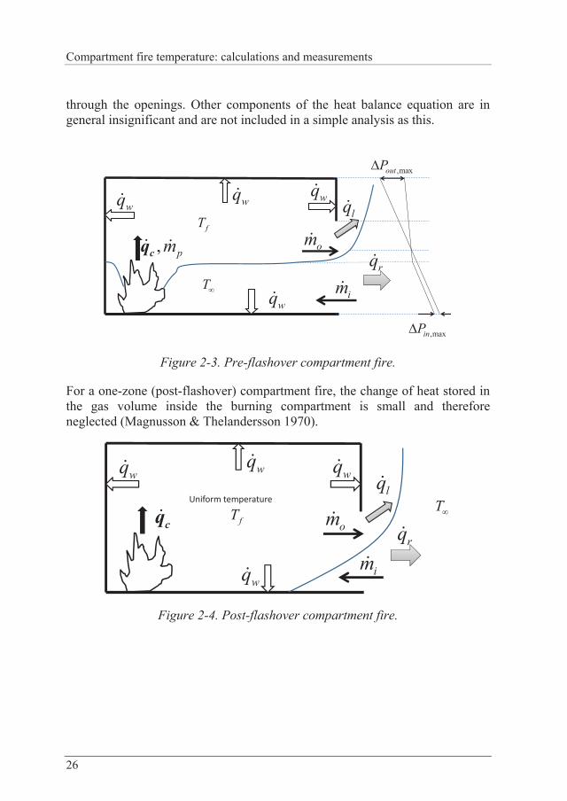
26

through the openings. Other components of the heat balance equation are in general insignificant and are not included in a simple analysis as this.

wqwq

wq

wq

, pmcq

lq

rqom

im

fT

T

,maxinP

,maxoutP

Figure 2-3. Pre-flashover compartment fire.

For a one-zone (post-flashover) compartment fire, the change of heat stored in the gas volume inside the burning compartment is small and therefore neglected (Magnusson & Thelandersson 1970).

wqwq

wq

wq

cqlq

rqom

im

Uniform temperature

fT T

Figure 2-4. Post-flashover compartment fire.


27

The combustion rate or the burning rate is computed as:

fuelc c

dmq H

dt (2.34)

where fueldmdt

is the mass burning rate of fuel, the combustion efficiency

and cH the complete heat of combustion, which is depending on the combustible materials. According to Tewarson (Tewarson 1980), the combustion efficiency values can be up to 93% for some liquid fuels, like heptane. This value has been determined in laboratory tests based on the measured heat of complete combustion of the fuel, using an oxygen bomb calorimeter and measuring the heat required to generate a unit mass of fuel vapors which has been obtained by so called pyrolysis experiments. A later work of Tewarson (Tewarson 1982), using a Factory Mutual flammability Apparatus, suggested that the combustion efficiency values can be up to 99% for methanol. By narrowing the range of the efficiency, the combustion efficiency is usually assumed to be in the range of 40% - 70% according to Drysdale (Drysdale 1998).

Combustion efficiency is an uncertain parameter. As a general rule it will decrease when fires become fuel rich or ventilation controlled as have been reported by for example Tewarson in 1980 (Tewarson 1980). Unburnt fuel may then burn outside the fire compartment.

The combustion rate cq inside a ventilation controlled (V.C) compartment is proportional to the mass flow rate and can be written as:

.2

V Cc aq m (2.35)

where 2 is a constant describing the combustion energy developed per unit mass of air (Paper B2, Paper B3). The combustion yield constant is assumed to be 6

2 3.0 10 (W·s)/kg. This value is obtained from the knowledge that most organic materials yield about 13.1·106 Ws per kg oxygen under ideal combustion conditions (Huggett 1980). The yield constant 2 is calculated assuming that the mass fraction of oxygen is 23 % in the ambient air.


28

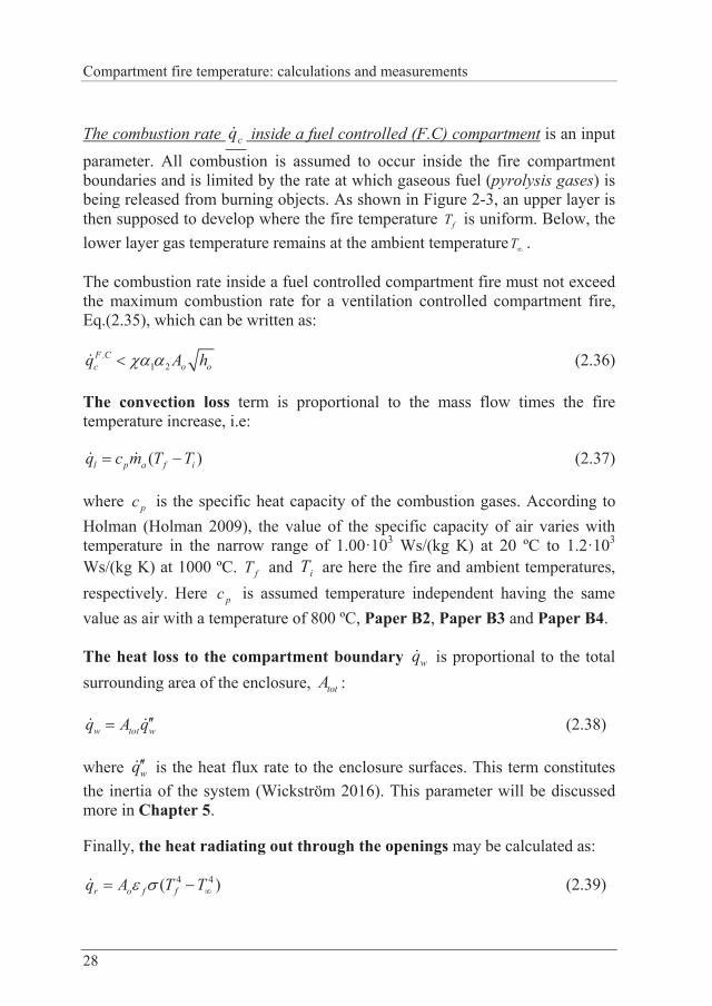
The combustion rate cq inside a fuel controlled (F.C) compartment is an input parameter. All combustion is assumed to occur inside the fire compartment boundaries and is limited by the rate at which gaseous fuel (pyrolysis gases) is being released from burning objects. As shown in Figure 2-3, an upper layer is then supposed to develop where the fire temperature fT is uniform. Below, the lower layer gas temperature remains at the ambient temperatureT .

The combustion rate inside a fuel controlled compartment fire must not exceed the maximum combustion rate for a ventilation controlled compartment fire, Eq.(2.35), which can be written as:

.1 2

F Cc o oq A h (2.36)

The convection loss term is proportional to the mass flow times the fire temperature increase, i.e:

( )l p a f iq c m T T (2.37)

where pc is the specific heat capacity of the combustion gases. According to Holman (Holman 2009), the value of the specific capacity of air varies with temperature in the narrow range of 1.00·103 Ws/(kg K) at 20 ºC to 1.2·103 Ws/(kg K) at 1000 ºC. fT and iT are here the fire and ambient temperatures, respectively. Here pc is assumed temperature independent having the same value as air with a temperature of 800 ºC, Paper B2, Paper B3 and Paper B4.

The heat loss to the compartment boundary wq is proportional to the total surrounding area of the enclosure, totA :

w tot wq A q (2.38)

where wq is the heat flux rate to the enclosure surfaces. This term constitutes the inertia of the system (Wickström 2016). This parameter will be discussed more in Chapter 5.

Finally, the heat radiating out through the openings may be calculated as:

4 4( )r o f fq A T T (2.39)


29

where T is the ambient temperature, assumed to be equal to the initial temperature, iT T , and the emissivity f is here a reduction coefficient considering that the entire opening is not radiating. For the one-zone (post-flashover) fire model a maximum value of f equal to unity can be assumed, see Paper B2 and Paper B3, for the two-zone (pre-flashover) compartment fire model a smaller value can be used, see Paper B4.

Flashover is generally defined as the transition from a growing fire, the so called pre-flashover fire, to a fully developed fire, a post-flashover fire, i.e. when all combustible items in the compartment are involved in fire (Walton & Thomas 2002). To define the onset of flashover one usually uses the value of the temperature in the hot smoke layer. In this case, temperatures in the range 500 to 600 ºC are often associated with the onset of flashover (Thomas 1981). Based on these characteristic temperature assumptions and applying the energy balance to the upper layer, several methods to predict flashover have been developed (McCaffrey et al. 1981; Babrauskas 1980; Thomas 1981). All these well-known models include losses to the compartment boundaries in the model.

In this study, flashover is supposed to occur when the combustible fuel gases balance the amount of oxygen available for combustion. Then the Heat Release Rate needed for flashover is:

. . 2 . . . 1 2F O a F O o oq m A h (2.40)

This criterion was used in the validation of experiments (Sjöström et al. 2016) with post and pre-flashover compartment fire.

Methods

31

3 METHODS

Different scientific research methods have been used in this thesis. The first part of this thesis, Paper A1, Paper A2 and Paper A3, focuses on understanding the theory of heat transfer to fire exposed surfaces and how this exposure can be measured. During this process several different experiments were conducted both in laboratory facilities and in the field. Temperature measurements were collected, analysed and applied as boundary conditions for the FE-analysis in Paper A3. The second part of this work, Paper B2, Paper B3 and Paper B4, focuses on the development of compartment fire models and validation of these models with experiments (Sjöström et al. 2016). During these experiments, temperature was measured with plate thermometers (PT) and thin thermocouples as a choice from the first part. All of the methods described in this chapter have been used in the research papers attached to this thesis.

3.1 Literature review

There are two main topics covered in this thesis: measuring techniques (PapersA) and compartment fire temperature model development (Papers B). Chapter 1 in this thesis contains a brief overview of references concerning the topics of compartment fire and measuring techniques in fire safety engineering. This literature study was a basis for understanding the idea of improving existing fire compartment models used for prediction of compartment fire temperature in enclosures. Improvements are obtained by going to the basic definitions of heat and mass balance inspired by the work done by Magnusson and Thelandersson in 1970’s (Magnusson & Thelandersson 1970). Chapter 2


32

contains a review of theories necessary for evaluating and analysing results of experiments conducted during this work. This includes understanding heat transfer at the exposed to fire surface, effect of thermal properties of surrounding structure and fire dynamics in compartment fires. Theories relevant for the specific aspects are presented and discussed in the appended papers, see Papers A and Papers B.

3.2 Experimental studies

The main purpose of all the experiments conducted in this thesis was to measure compartment fire temperatures and thermal exposure of structures. Plate Thermometers and thin thermocouples were studied in laboratory facilities Paper A1, in the field, Paper A2 and Paper B1, and inside a turbulent flame, Paper A3.

3.2.1 Experiments in laboratory facilities

Experiments conducted at laboratory facilities are usually more controlled and give the opportunity to study effects of different parameters, such as heat release rate or incoming radiation. Furthermore, they usually have more information about the thermal material properties used in the experiments.

Cone calorimeter (Paper A1)

These experimental studies were conducted in the laboratory facilities at Luleå Technical University in the experimental laboratory Complab. The main focus was to study the use of the concept of adiabatic surface temperature (AST), based on the measured temperatures with Plate Thermometers (PT) according to ISO 834 (ISO834-1 1999) and EN 1363-1 (EN1363-1 2012) and thin thermocouples (Ø=0.25 mm). The purpose of these studies was to get better understanding of how we can predict and describe in a quantitative way the thermal exposure of structures in mixed boundary conditions, see Chapter2.1.3.

The experiment was conducted in a cone calorimeter (ISO5660-1 2002) under constant incident radiation heat flux exposure, see Paper A1. Temperature was measured with three devices: a quick-tip 0.25 mm in diameter and a shielded thermocouple (TC) with an outlet diameter of 3 mm attached to the PT, see Figure 3-1. The PT and thermocouples were placed 20-25 mm under the edge of the radiation heater in a cone calorimeter and exposed to a constant incident

Methods

33

radiation heat flux of 25 kW/m2 and constant gas temperature. Natural convection boundary conditions were assumed for the horizontal plate.

(a) (b)

Figure 3-1. (a): Cone calorimeter ISO 5660 (ISO5660-1 2002), (b) Plate Thermometer together with a thermocouple.

Fire testing laboratory at SP, Borås

Experiments referred in this part were carried out in the large fire hall of the fire testing facilities, SP, Borås, Sweden. The size of the hall is 20 m by 20 m and 20 m high.

Localized fire (Paper A3)

A 6 m tall, 200 mm wide and 10 mm thick circular, unprotected and unloaded steel column was exposed to circular pool fires with various burning area, see Figure 3-2. This column was hanging centrally fixed at the upper end, 200 mm over the fuel container in the middle of the fire hall under the main exhaust hood. The lower and upper ends of the column were sealed (for more details about the experimental setup, see Paper A3 and the technical report (Sjöström et al. 2012). The main objective of this experiment was to measure thermal exposure of a structure with PTs and investigate if these measurements could be used as boundary conditions for calculating temperature in structures exposed to localized fires.


34

(a) (b)

Figure 3-2. Setup for localized fire experiment: (a) steel column, position of thermo devices, (b) large fire hall at SP, Sweden.

Gas temperatures were measured using welded 0.25 mm thermocouples. Steel temperatures were measured with thermocouples fixed about 1 mm into the steel structures. Standard plate thermometers were used as in furnace testing according to EN 1363-1 (EN1363-1 2012). They were mounted a few centimetres from the steel surface. In two positions, ±90° from position 1, curved PTs were mounted in square holes in the steel column together with thin thermocouples, see Figure 3-3. Opposite to position 1, gas and steel temperatures were measured together with PTs at 2 m and 4 m heights, see Figure 3-3. The experiment setup is described in details in Paper A3 and in a technical report (Sjöström et al. 2012).

Methods

35

(a) (b)

Figure 3-3. Localized fire (a) experimental setup seen from position 1(b): cross section of the column from top view showing instruments in the different positions, Paper A3.

Room fire

A set of experiments in reduced scale was conducted at the SP Fire Research (Sjöström et al. 2016). These experiments using constant effect from the burning source were chosen for validation of the room fire models described in Paper B3 and Paper B4. The experiments were conducted in a compartment with light weight boundaries and in a compartment having steel boundaries both with and without insulation. For more data and information about the experimental setup and result, see report (Sjöström et al. 2016). The main objective of these experiments was to collect data for validation of the pre- and post-flashover models described in this thesis, see Chapter 5.

The inner structure was representing an office room in scale 3:4. The inner dimensions of the tested compartment were 1800 mm by 2700 mm having a height of 1800 mm. Centrally on one of the short ends was a 600 mm by 1500 mm high doorway opening. The materials and thicknesses of the walls were changed between the test series (Sjöström et al. 2016). The same materials were used in floor, ceiling and walls for each set of experiments.

To minimize uncertainties due to effect produced by the burning source, a gas burner with a known mass flux output was used in these experiments. A


36

diffusion propane burner (300 mm by 300 mm) was placed in the middle of the enclosure. The gas burner was filled to half its volume with gravel (~10-20 mm stones). The heat release rate (HRR) was kept constant at 500 kW (defined as a pre-flashover room fire according to the theory described in Chapter 2.2.2) and 1000 kW (post-flashover room fire).

Several thermocouple trees were installed to measure gas temperatures at various heights (Sjöström et al. 2016). Insulated Plate Thermometers (insPT) (Sjöström & Wickström 2013) together with thermocouples were mounted both inside the compartment and in the door opening. In total, more than 50 measuring devices were installed during each experiment. In this work, only the readout from the insulated Plate Thermometers (insPT) measurements were selected and compared with calculated fire temperatures. In addition, some PT measurements were correlated to the AST. This correlation procedure will be more discussed in Chapter 4.3.

3.2.2 Experiments in the field

The main focus of the experimental studies conducted at the Luleå Emergency Training Center (Luleå Räddningstjänst utbildningscentrum), was to study the use of the concept of adiabatic surface temperature (AST) based on measured temperatures with Plate Thermometers (PT) and thin thermocouples (Ø=0.25 mm) in full scale experiments under field conditions. The purpose was to get better understanding of how we can predict and describe in a quantitative way the thermal exposure of structures in a two-zone compartment fire.

Steel container (Paper B1)

Two pool fire tests were conducted in a non-insulated steel container in the field under low ambient temperature conditions, -20ºC, see Paper B1. The inner dimensions of the steel container were 12000 mm by 2400 mm, a height of 2400 mm and with a steel thickness of 3 mm. The floor was made of concrete. Centrally on one of the short ends was an 800 mm by 2000 mm high doorway opening, see Figure 3-4.

A steel fuel tank was located 1.0 m from the closed end of the container. The size of the tank was 0.7 m by 0.7 m and 0.2 m deep. The mass loss rate of the burning jet fuel was measured. The heat release rate was calculated by multiplying the mass loss rate by the effective heat of combustion of the jet fuel, which was assumed to be 43000 kJ/kg. Seven temperature devices,

Methods

37

including five high temperature thermocouples (HT) and two plate thermometers (PT), were installed on the wall to measure temperature.

Figure 3-4. Setup for full scale experiment, Paper B1.

Two-story concrete building (Paper A2)

This full scale experiment was conducted in a two-story concrete building connected with a stairwell during a day with very low ambient temperature. Four thermocouple trees and five plate thermometers measured gas temperatures and adiabatic surface temperatures in the compartment. The mass loss of fuel (wooden cribs) was recorded during the test. The AST was then derived based on the measured temperatures by PT and TC (0.25 mm). In addition, FDS simulations of the fire scenario were carried out.

Temperatures measured by PT were compared with the gas temperature measured by ordinary thermocouples (TCs). These experiments were conducted in full-scale, see Paper A2. The AST calculated from temperatures measured by plate thermometer was compared with the AST calculated by the CFD code FDS. Good agreements between the ASTs based on measurements and those based on FDS computations, respectively, were obtained.

Figure 3-5 shows the concrete building used for this experiment. It is normally used for the daily training of fire-fighters. The main part is a 2 story building, connected via stairwell (the highest part of the building). The experiment was conducted in the compartment on the ground floor. The door to the compartment above from the stairwell was kept closed.


38

Figure 3-5. The concrete building.

The temperatures were measured by TCs together with PT. The location of the TCs are as shown in Figure 3-6. TCs together with PTs on positions 1, 2, 4, 5 were mounted on the height 1.6 m, see Figure 3-6. PT 5 and TC-5 were placed on the ground level facing upwards 1 m away from the fire source.

The setup of the experiment together with detailed information about fuel and positions of the measuring devices can be found in Paper A2 and (Byström et al. 2012).

Figure 3-6. Positions of the thermocouples TC and plate thermometers PT.

Methods

39

3.3 Computation models for compartment fire

Based on the theory described in Chapter 2, a new formulation to calculate the smoke fire temperature has been developed for both pre-and post-flashover fire scenarios, Paper B2 and Paper B4, respectively.

The pre-flashover and post flashover fire models presented in Chapter 5, Paper B2 and Paper B4 are inspired by the work of Magnusson and Thelandersson (Magnusson & Thelandersson 1970). The fire temperature as a function of time according to the proposed models may in some idealized cases be calculated by simple analytical closed form expressions. These models are based on energy balance within a single fire compartment, see the theory described in Chapter 2.

The new approach presented in this thesis may use finite element modelling for calculating fire temperature, see Paper B3 and Paper B4. It gives the opportunity to accurately consider the influence of various boundaries including structures containing several layers, materials with temperature dependent properties as well as voids where radiation and convection heat exchanges are considered. Thus non-linear effects due to latent heat caused by water evaporation may for example be considered. Previous models are not able to accurately consider such effects. By making certain approximations, simple spread-sheet calculations may be used for calculating the fire temperatures and even closed form analytical solutions may be derived, see Paper B2, Paper B4 and (Wickström 2016). In general, this model shows that the maximum temperature is only slightly dependent on the fire compartment geometry while the rate at which the fire temperature rises is increasing by the ratio of the opening factor and the thermal inertia of the surrounding boundaries.

3.4 Numerical modelling

Finite element modelling: TASEF It is common to use finite element analysis in heat transfer problems. Several computer codes are commercially available for calculating temperature in fire exposed structures. In general, modern codes are based on the finite element method. Some are specifically developed and optimized for calculating temperature in fire exposed structures while others are more general purpose codes. TASEF (Wickström 1979a; Sterner & Wickström 1990), SAFIR (Franssen 2005) and others are example of programs which have been


40

developed for fire safety problems. They all allow for temperature-dependent material properties and boundary conditions.

There are many very advanced general purpose finite element computer codes commercially available like ABAQUS, ANSYS, ADINA and COMSOL. These codes can be used for many types of problems including three-dimensional heat transfer and they all come with advanced graphical user interfaces and postprocessors.

All the FE-analysis in this thesis was done by using a software called TASEF (Temperature Analysis of Structures Exposed to Fire) (Wickström 1979a; Sterner & Wickström 1990). TASEF is capable of solving one- and two-dimensional, axisymmetric heat transfer problems. The TASEF code was designed in the late 70s but has in later years got the interface TASEFplus.

TASEF employs a forward difference solving technique which makes it particularly suitable for problems where latent heat due to e.g. evaporation of water must be considered. It requires in most cases very short computing times, in particular for problems with a large number of nodes.

The boundary conditions that can be defined in TASEF are shown in Table 2-1, including natural or third kind boundary conditions with different exposure gas and radiation temperatures.

Finite difference – Computational Fluid Dynamics (CFD) Additional simulations were performed using the Fire Dynamics Simulator (FDS) (McGrattan et al. 2015b), see Paper A2, Paper B1 and Paper B3. The FDS software solves the Navier-Stokes equations in the limit of low-speed, thermally-driven flow with an emphasis on smoke and heat transport from fires. The algorithm used is an explicit predictor-corrector scheme that is second order accurate in space and time where turbulence is treated by means of Large Eddy Simulation (LES). The FDS software with default settings uses a structured, uniform staggered grid in order to utilize the efficiency of the Fast Fourier transforms in the pressure solver. The combustion chemistry is simplified and a generalized lumped species approach together with the eddy dissipation concept is used for a single step reaction between fuel and oxidizer. In the default setting, radiation is calculated using 100 discrete angles in a finite volume approximation of the radiation transport equation with grey gas. The FDS model is not limited to these simple algorithms, however any additional physics included incur at increased computational costs. The default

Methods

41

model options have been selected in some cases based on results from a wide variety of full-scale validation experiments (McGrattan et al. 2015a).

All simulations have been done in accordance with the tests using the same heat release rates and geometrical set-up and extracting similar outputs as in the experimental scenarios. The material data (in cases when known) (PaperB3) was taken from measurements.

For some studies, the FDS output Adiabatic Surface Temperatures was compared with AST calculated from PT measurements (Paper A2 and Paper B1). In Paper B3, plate thermometers were introduced as physical objects in the simulation to be able to account for the time delay of the PT response depending on the thermocouple characteristics of the insulating material and the sheet of metal in the plate thermometer. The physical model of PT described by Jansson and Anderson (Jansson & Anderson 2012) was used for the FDS simulation in Paper B3.

3.5 Influence of various parameters

The numerical and analytical models described in this thesis require assumptions for some parameters. The effects of different parameters in one of these models were studied and presented in the licentiate thesis (Byström 2013). The main objective was to see how these parameters affect the final fire temperature in the compartment.

Measuring techniques

43

4 MEASURING TECHNIQUES

When designing a structural element it is very important to estimate the right temperature to which such elements can be exposed. This can either be done experimentally or numerically.

In fire safety engineering, temperature is nearly always measured with thermocouples. However, all types of thermo devices measure strictly neither the gas temperature nor the radiation temperature, but rather a weighted average in between. As shown in Paper A1, there is a great difference in temperatures measured by different thermo devices, see Table 4-1. Similar observations were made in Paper A2, Paper A3 and Paper B1.

Table 4-1. Measured temperatures in a Cone Calorimeter with various devices. Summarized results presented in Paper A1.

Thermo device Temperature after 500 sec. [ºC]

Plate Thermometer (PT) About 500

Thermocouple Ø=0.25 mm About 60

Shielded thermocouple Ø=3 mm About 160

This chapter contains an overview of different thermal devices often used to measure thermal exposure and the theory behind how these measurements can be used. The main focus was the use of the concept of adiabatic surface


44

temperature (AST) based on measured temperatures with Plate Thermometers (PT) and thin thermocouples (Ø=0.25 mm). Several experiments were conducted in various fire conditions. The measurements were done under constant incoming radiation heat flux and constant gas temperature in a cone Calorimeter (Paper A1), during experiments in full-scale tests in the field (Paper A2) and during local exposure from a flame (Paper A3).

The purpose of these studies was to get better understanding of how we can predict and describe in a quantitative way the thermal exposure of structures during any set of experiments.

4.1 Thermocouple

A thermocouple is two wires of different metals or alloys connected at two points. A voltage is then generated proportional to the temperature difference between the so called hot junction and the cold junction, a reference point with known temperature.

There are several different types of thermocouples widely used in fire safety engineering. In this work, different designs of thermocouples in fire safety engineering have been divided into the following four main categories:

Bare bead thermocouples (TC) are widely used in various fire applications for many reasons. They have low cost, wide temperature range (depending on the type of metal combination), are robust and easy to replace. However, a thermocouple measurement is subject to uncertainties related to its bead size, time response and radiation effect on the measured temperature (Whitaker 1972; Pitts et al. 1998; Blevins & Pitts 1999; Hamins et al. 2006).

High temperature (HT) thermocouples with ceramic protection tube are often used in combustion boilers and heat treatment furnaces. Due to ceramic protection, this type of thermocouple is designed to meet the most demanding temperature requirement. This kind of thermocouples were used during the experiment in the steel container, see Paper B1. The measured temperatures were corrected to eliminate the effect of thermal inertia (slow response of HT). However, a HT measurement (similar to a bare bead TC) is subject to uncertainties related to its bead size, time response and radiation effect on the measured temperature.

Aspirated thermocouple, also known as suction pyrometers. Several papers have been published on the design and use of aspirated thermocouples, also


45

known as suction pyrometers (Strömberg 1975; Pitts et al. 1998; Blevins & Pitts 1999; Blevins 1999; Sung Chan Kim & Hamins 2008).

Aspirated thermocouples are more accurate for measuring gas temperature in a highly radiating environment than bare-bead thermocouples. Aspirated thermocouples can be used for uncertainty estimates for bare-bead thermocouple temperature measurements (Brohez et al. 2004).

Thermocouples integrated into the surface of structural elements are used in order to be able to measure temperature on the surface of exposed structures. However, this can only be done on metal structures. This is often achieved by welding bare bead thermocouples to the metal surface or by using thermocouples with quick-tip placed into drilled holes and fixed by a punch mark in the nearby metal (Sjöström et al. 2012).

4.2 Heat flux meter, HFM

For several purposes, the incident heat radiant flux can be important to know. Radiative heat flux is usually measured with so-called total heat flux meters of the Schmidt-Boelter (thermopile) or Gardon (foil) types. Such meters register the combined heat flux by radiation and convection to a water cooled surface. The flux by convection will, however, depend on the size and shape of the heat flux meter, its orientation, and its temperature level, which is near the cooling water temperature. In many practical situations in fire testing, uncertainties due to convection can amount to 25 % of the total heat flux, see ISO 14934 (ISO14934-1 2010).

According to Wickström (Wickström 2016), the heat flux meter is exposed to both convection and radiation so the general expression of the heat flux meter is:

'' '' 4hfm hfm inc hfm hfm g hfmq q T h T T (4.1)

where hfmT is assumed equal to the cooling water temperature, hfm is emissivity, gT the gas temperature near the HFM and hfmh is the convective heat transfer coefficient at the surface of the HFM.

A heat flux meter is a very sensitive device. In 1997, Persson and Wetterlund, (Persson & Wetterlund 1997) concluded that the convective influence of a heat flux meter can be quite different depending on the arrangement of the meter


46

and the heating source. A heat flux meter mounted in free air allowing cool air to pass the sensing element will register a too low heat flux. On the other extreme, a heat flux meter mounted in a surrounding board which is heated by incident radiation will register a too high heat flux. More complete analyses of the use of heat flux meters are given in the following publications (Lattimer & Thomas Diller 2011; Lattimer 2016).

4.3 Plate thermometer

So called plate thermometers measure approximately the adiabatic surface temperature (AST), which is a suitable quantity when modeling heat transfer from fires to structures in fire. The concept of AST was discussed earlier in Chapter 2.1.5. As stated above in Chapter 2.1.5, the AST is a weighted mean temperature of the radiation temperature and the gas temperature. It is possible to measure the AST with plate thermometers (PT) (Wickström 1994; Ingason & Wickström 2007) or numerically calculate it by using the computer code FDS (McGrattan et al. 2015b; Sandström 2013).

4.3.1 Alternatively designed Plate Thermometers

The Plate Thermometer was invented to measure and control temperature in fire resistance furnaces (Wickström 1994). The standard design PT is specified in the international and European standards ISO 834-1 (ISO834-1 1999) and EN 1363-1 (EN1363-1 2012). It is made of a shielded TC welded to the center of a 0.7 mm thick nickel alloy sheet folder which is insulated on its back side. The exposed front face is 100 mm by 100 mm and has on the backside a 10 mm thick inorganic insulation pad, see Figure 4-1. The plate thermometer is sensitive to convection and radiation in a similar way as a real specimen, due to large sensor surface. Therefore it yields an effective temperature which can be used for predicting the heat transfer to surfaces exposed to radiation and convection. This suggests that PT measurements yield very valuable data for expressing the intensity of thermal exposure which was earlier shown for a beam (Wickström et al. 2009). In that case, temperatures measured with PTs and thermocouples, respectively, were very different.


47

Thermocouplewelded on the

back side

Thermocouplelead

Sensor surface

Insulationpad

Figure 4-1. Design of a Plate Thermometer.

Plate thermometers can be of various designs, but they always consist of three main components: a relatively large metal sensor surface, insulation and a thermocouple welded on the back side of the sensor surface, see Figure 4-1. The sensor surface size or shape can be varied depending on the geometry of the target surface.

To minimize errors in the measurements and make it possible to evaluate measured data, the following parameters should be kept in mind:

1. The thinner the sensor plate, the faster the response time of the device.

2. The emissivity of the exposed surface is important.

3. Geometry and size of the sensor surface affects the heat transfer coefficient by convection, ch . The bigger surface, the lower value of ch (Holman 2009; Wickström 2016).

4. The insulation on the back side reduces the heat losses from the sensor surface.

Alternatively designed PTs, that can be found in the literature:

Standard PT, Insulated PT (insPT) or Plate Thermometer. The insPT is designed to improve the calculations of incident radiation (Sjöström & Wickström 2013). Compared to a standard PT, the insPT is better insulated


48

having 30 mm ceramic wool compared to 10 mm for a standard PT. The ceramic wool has lower density which minimizes the heat capacity of the device. A thinner Inconel steel plate (0.4 mm) and less metal is used to attach the insulation pad, see Figure 4-2.

Figure 4-2. Plate thermometers (non-standard) mounted in two directions, adapted from (Sjöström & Wickström 2013).

A Heat Flux Meter (PTHFM) is a modified and improved version of an insulated PT (insPT). The PTHFM was developed for measuring incident radiant heat flux up to 80 kW/m2. The PTHFM consists of a thinner Inconel steel plate (0.3 mm) having a high surface emissivity of about 0.95. This type of PT is still under development and improvement.

Copper disk PT (cdPT). This is a kind of plate thermometer developed to estimate AST. The cdPT consists of a small copper disc with a diameter of 12 mm in contrary to the standard PT. This device has been named copper disc plate thermometer (cdPT), (Denisse 2011). This new smaller PT is easy to produce, can be mounted within the sample and will continue to work even when the sample ignites (Denisse 2011; Byström et al. 2015).

Specifically designed PTs. There are other varieties of plate thermometer devices. Some examples of specifically designed PTs found in the literature are:


49

- a cylindrical shape PT imitating munitions exposed to fire (Evers & Möllerström 2013),

- a car replica (0.5 m by 1.5m Inconel plate, insulated on the backside, equipped with seven thermocouples on the backside), used when studying fire spread in tunnels (Sjöström & Wickström 2013),

- a bent steel plate insulated on the back side has been integrated inside a steel column exposed to localized fire, see Paper A3.

4.3.2 Corrections of PT measurements

The use of PT to calculate incident heat flux was first described by (Ingason & Wickström 2007). It requires the knowledge of the surface emissivity, an estimation of the convective heat transfer coefficient and the ambient gas temperature during the experiment.

The dynamic heat balance at the exposed surface of a PT may be written as:

4 PT PTinc PT c g PT PT g PT PT

dTq T h T T K T T Cdt

(4.2)

where PTT is the temperature measured by PT in Kelvin. Here

- PTK [W/m2K] is the heat conduction coefficient of the PT. This is a correction factor due to heat losses by conduction from the sensor surface of the PT. Heat is conducted through the insulation in the metal holder and lost by radiation and convection on the backside of the PT (Häggkvist et al. 2013; Sjöström & Wickström 2013).

- PTC [J/m2K] is the heat capacity coefficient. This is a correction factor due to the heat being stored in the PT when the temperature rises in the metal and insulation slab (Häggkvist et al. 2013; Sjöström & Wickström 2013).

Values of the correction factors for some PT have been analysed both experimentally and through finite element analysis (Häggkvist et al. 2013; Sjöström & Wickström 2013) and can be found in Table 4-2.


50

Table 4-2. Correction factors for PT measurements, according to Sjöström and Wickström (Sjöström & Wickström 2013).

Type of plate thermometer Correction factor

for conductive losses, K , W/m2K

Correction factor for thermal storage,

C , J/m2K

Standard PT, ISO 834-1 and EN 1363-1 8 4200

Copper disk PT (cdPT) 6 1240

Insulated PT (ins PT) 4 2500

Incident radiation from PT measurements

Heat balance at the surface of the PT, Eq.(4.2), can provide the incident heat flux (Häggkvist et al. 2013; Sjöström & Wickström 2013).

4

PT PTc PT g PT PT

inc PT

dTh K T T Cdtq T (4.3)

Adiabatic Surface Temperature from PT measurements

The temperature measured by a PT is close to the AST. However, there are some differences between them due to the response time and the heat conduction loss of the PT. Based on the theory in Chapter 2.1.5, the AST can be calculated based on the measured temperatures by PT, PTT , together with the gas temperature, gT , according to Eq. (4.4). A more detailed procedure is presented in Paper A2.

PTPT PT g PT

AST PT PT PTr c

dTC K T TdtT T

h h (4.4)

where


51

2 2PTr AST PT AST PTh T T T T (4.5)

In the Cone Calorimeter experiment in Paper A1, temperatures measured by the finest thermocouple (Ø =0.25 mm) were much closer to the gas temperature than to the radiation temperature. These kinds of thermocouples are quite sensitive to heat transfer by convection and relatively less sensitive to radiation due to thermocouples geometry and relatively small size. In this thesis, it has been assumed that the finest TCs give values close to the gas temperature.

Comparison results show that the calculated AST increases more rapidly than the measured temperature of the PT during the initial growth period. However, the AST and measured temperature with PT agree well during the steady state period, see Paper A2.

The calculated values of AST can thereafter be used as input to finite element calculations of the thermal exposure of any surface or construction elements, see Paper A3. The measured and simulated (with use of FE analysis) values of the steel temperatures match very well despite the unstable and inhomogeneous nature of the flame, see Paper A3.

Compartment fire models

53

5 COMPARTMENT FIRE MODELS

The models described in this thesis are based on an analysis of the energy and mass balances in fire compartments. The mathematical formulations include key physical and chemical input parameters. The theory covered in Chapter2.2 of this thesis describes the fundamental principles underlying compartment fire temperature development. Based on these theories, models for pre- and post-flashover compartment fires have been modified as presented in PaperB2, Paper B3 and Paper B4.

It is demonstrated in the attached Paper B2, Paper B3 and Paper B4 that these models can be used to predict fire temperatures in compartments with boundaries of semi-infinitely thick structures as well as with boundaries of insulated and non-insulated steel sheets where the entire heat capacity of the surrounding structure is assumed to be concentrated to the steel core. With these assumptions, fire temperatures can be calculated using spread-sheet calculation methods. For more advanced problems, a general finite element (FE) solid temperature calculation code (TASEF) was used to calculate the temperature in the boundary structure, see Paper B3 and Paper B4. With this FE code it is possible to analyse surrounding structures of various kinds, for example comprising materials with properties varying with temperature as well as assemblies of various materials and voids.

It is also shown how these models relate to current standard time-temperature curves, so called parametric fire curves, see Paper B2 and Paper B3. In PaperB3 and Paper B4, these models were validated with a series of accurately defined experiments. In all these tests, a propane diffusion burner was used as the only fire source. Temperatures were measured with thermocouples and plate thermometers at several positions (Sjöström et al. 2016).


54

The objective of the work presented in this chapter is to discuss some novel techniques to calculate fire temperature in enclosures with any boundaries for both pre- and post-flashover fire scenarios. These models are able to take into account the effect of radiation losses through openings and heat loss out through the compartment boundaries of any layer (multiple layers with temperature dependent material properties).

5.1 Limitations

A number of simplifications and assumptions are made to limit the number of input parameters and facilitate the calculations. These are

- The fire compartment is ventilated by natural convection at a constant rate in terms of mass per unit time, independent of temperature.

- The combustion rate inside a ventilation controlled compartment is limited by the amount of available oxygen, i.e. proportional to the ventilation rate. The combustion rate inside a fuel controlled compartment is an input parameter. This parameter was discussed early in Chapter 2.2.2 of this thesis.

- The gas temperature of the fire hot layer is uniform in the fire compartment.

- The fire duration is proportional to the amount of energy in the combustibles in the compartment, i.e. the fuel load, over the ventilation rate for ventilation controlled fires.

- The energy of the fuel is released entirely inside the compartment.

- For analytical solutions, all material and physical parameters (heat transfer coefficients, heat release rate, etc.) are assumed constant

5.2 Compartment fire models

The post-flashover fire model is mainly inspired by the work of Magnusson and Thelandersson (Magnusson & Thelandersson 1970), which was later modified and reformulated in a work by Wickström (Wickström 1985).

In the post-flashover model, the heat release rate cq is proportional to the mass flow rate of air into the compartment which in this case is constant, see Paper


55

B2 and Paper B3. Fire burns at its maximum potential of the available air supply and any unburned fuel vapors leaving out through the openings will burn outside the compartment. The temperature inside an enclosure is assumed uniform and the air flow into the compartment depends on the geometry of the openings (area times the square root of the height).

In the pre-flashover model, the heat release rate cq (kept constant) is an input parameter, see Paper B4. The entire combustion is assumed to occur inside the fire compartment boundaries and is limited by the rate at which gaseous fuel (pyrolysis gases) are being released from burning objects. As shown in Figure 2-3, the upper layer is then supposed to develop a uniform fire temperature. In the lower layer, the gas temperature remains at the ambient temperature. The heat is assumed lost to all compartment boundaries uniformly. This is justified by the fact that the heat transfer to the surrounding surfaces is dominated by radiation which is independent of gravity.

Hot gases generated by the combustion enter the upper layer via the fire plume. Ambient air is continually entrained over the plume height. The flow rate at which mass is entering the upper layer is assumed to govern the mass flows in and out of the compartment, see Paper B4.

5.3 Analogous electrical model

The thermal conditions of a one dimensional heat transfer system can be seen as an analogous electrical circuit (Wickström 2016; Holman 2009). This electrical analogy has here been used to illustrate and explain heat transfer in the development of room fire models, Paper B2, Paper B3 and Paper B4. For that reason, the heat balance equation of a compartment fire was rearranged analogously to the heat transfer equation by convection and radiation between a gas and a solid surface.

Heat transfer in fire safety engineering according to the theory described above in Chapter 2.1.2 and Chapter 2.1.1 from a fire to any surface occurs by convection and radiation according to

'' '' ''tot rad conq q q (2.14)

By assuming natural/mixed boundary conditions (see Table 2-1), heat transfer at any surface can be expressed by using characteristic temperatures, the so called radiation, gas and surface temperatures:


56


5.3.1 General formulation of the new fire models

By rearranging the heat balance equation Eq. (2.33) for pre- and post-flashover compartment fires, we get:

- Post-flashover energy balance equation, Paper B2 and Paper B3:

4 4 21( )o

w f p ftot p

Aq T T c OA c

(5.1)

- Pre-flashover energy balance equation, Paper B4:

51 23 3 334 4

53

3

( )o f p c cw f f

tot tot p

A c q z qq T TA A c z

(5.2)

where all the parameters of the heat balance equation have been discussed earlier in Chapter 2.2 of this thesis.

Eq. (5.2) and Eq. (5.1) are analogous to the heat transfer equation by convection and radiation between a gas and a solid surface Eq. (2.15) and may be seen as an analogous electrical model as shown in the figure below in Table 5-1, on the left part.

These new methods introduce the so called ultimate fire temperature, which is the highest temperature that can be reached when there is no energy lost to the compartment surrounding structures and out through the openings by radiation. The ultimate compartment fire temperature will not be obtained in reality as fire compartments have openings where heat will be lost by radiation. Exceptions may be furnaces and tunnels which have no openings directly to areas at ambient temperatures. In those cases, very high temperatures might therefore develop. The ultimate compartment fire temperature is introduced here to facilitate the derivation and explanation of the fire temperature development model. Notice that the ultimate temperature used in the pre-flashover model is not the same as the ultimate temperature defined for the post-flashover compartment fire model. For a pre-flashover compartment fire, the ultimate fire temperature has here been named the ultimate compartment fire temperature rise with a prescribed heat release rate. By definition, this


57

temperature must be less than the ultimate fire temperature for a post-flashover fire.

Let us now assume that the compartment has perfectly insulated boundaries, i.e. no heat loss by conduction through the boundaries. However, heat is lost by radiation out through the opening(s) into the ambient environment. Then the two temperatures ultT and T can be reduced into one resultant maximum fire temperature maxT , see Table 5-1. The maximum fire temperature can be defined as a weighted mean value of ultT and T , see Paper B2 and Paper B4. This can be done in a similar way as in the theory behind the adiabatic surface temperature (Wickström 2016).


58

Table 5-1. Comparison between the pre- and post-flashover models.

Post-flashover fire model

Paper B2 & Paper B3

Pre-flashover fire model

Paper B4

Governing formulation in form of a heat transfer equation for natural/mixed boundary conditions, Chapter 2.1.5,

'' 4 4( ) ( )tot s r s c g sq T T h T T

.f cR.i cR

ultT

fT sT

wq

Surroundingstructure

.i rR.f rRT

. .

1 1( )w f ult ff r f c

q T TR R

Fire compartment artificial thermal resistance due to radiation heat transfer

. 2 2.

1 1ˆf r

f r f f

Rh T T T T

where ˆ is a so called analogous emissivity

ˆ o f

tot

AA

in which the emissivity f here is a reduction coefficient considering that not the whole entire opening is radiating in contrary to the one-zone fire model

f assumed unity Lower value can be assumed ( 0.5f , Paper B4)


59

Post-flashover fire model

Paper B2 & Paper B3

Pre-flashover fire model

Paper B4

Fire compartment artificial thermal resistance due to convective heat transfer

.. 1

1 1f c

f c p

Rh c O

Opening factor o o

tot

A hO

A

*. 51*

3 3. 3

1 totf c

f c p c

ARh c q z

z is the maximum effective height of the plume above the burning area

Ultimate fire temperature rise - the highest temperature that can be reached in a compartment where the heat loss by radiation and heat loss into the boundary can be neglected.

2ult

pc

23

*5

33

cult

p

q

c z

Maximum fire temperature rise - the highest temperature that can be reached in a compartment where the heat loss into the boundary can be neglected.

max 2 2

1

ˆ ˆ( )( )1

ult

f f

p o

T T T Tc h

*

*max 2 2

513 3

3

ˆ ˆ( )( )1

ult

o f f f

p c

A T T T T

c q z

5.3.2 Heat transfer at the surface of the surroundings

The general formulations of the fire compartment models, i.e. Eq. (5.2) and Eq. (5.1), are expressed using the key parameter wq , which is the heat flux rate to the enclosure surfaces. Thus the heat transfer to fire compartment surfaces can be seen as an analogous electrical model, as shown in the figure in Table 5-1.

ultT and T can here be combined into an efficient temperature maxT . The two plus two parallel resistances can be combined into two resistances in series, see Figure 5-1.


60

max.f totR .i totR

maxTfT sT

.f cR.i cR

fT sT

wq


.i rRmax.f rR

maxT


Figure 5-1. Electric circuit analogy model of a fire compartment boundary according to the new model

These two can further be combined into one by adding them together. Thus a third kind of boundary condition (Wickström 2016) is defined as discussed in Chapter 2.1.3). This has been formulated and discussed in more detail in Paper B2, Paper B3 and Paper B4.

5.4 New calculation models

Pre- and post-flashover compartment fire models for three levels of complexity have been developed and reported in this thesis: a hand-calculation model (with closed form analytical solution) and a numerical approach with two levels of complexity.

The heat transfer through the boundary has a major influence on the compartment fire temperature. In particular, two types of analysis depending on boundaries have been performed in this thesis:

- boundaries of semi-infinitely thick structures

- boundaries of insulated and non-insulated steel sheets where the entire heat capacity of the surrounding structure is assumed to be concentrated to the steel core.

5.4.1 Analytical solution

Usually compartment boundaries may be considered thermally thick as the fire durations are relatively short. Based on this assumption and in analogy with the


61

general solution of the surface temperature of a semi-infinite body (Holman 2009), a formulation for the fire temperature development in a fire compartment surrounded by semi-infinite structures has been proposed.

Another analytical solution of the fire temperature was obtained when the fire compartment is surrounded by structures consisting of a metal core where all the heat capacity is concentrated. Thus the capacity per unit area coreC may be approximated as lumped into the core.

The analytical solutions are possible only when all involved materials and physical parameters (heat transfer coefficients) are assumed constant. A detailed procedure of how to find an analytical solution for pre-flashover and post-flashover can be found in Paper B2 and Paper B4, respectively.

The analytically derived time-temperature development for the semi-infinite compartment boundary correlates well with the corresponding curves given in Eurocode 1 (EN1991-1-2 2002) as parametric temperature-time curves, see Paper B2.

5.4.2 Numerical solutions

More accurate solutions for the core temperature and fire compartment temperature can be obtained by the step-by-step numerical procedures described in Paper B2 and Paper B4. Then material properties and in particular the heat transfer conditions can be updated at each time step. In the case of structures where lumped heat can be assumed, the core and fire temperature can be calculated numerically by a forward difference method, which can be coded into MS-Excel or MATLAB applications.

The purpose of using finite element modeling is to consider resistances varying with temperature due to radiation as well as material properties varying with temperature. More complex surroundings like voids inside walls (Byström 2013), effects of moisture in the boundary structure etc. can then be considered.

To calculate surface temperatures according to the theory described in PaperB3 and Paper B4, the finite element code TASEF (Wickström 1979b) was used. Due to the experimental setup (the same material of the walls, ceiling and floor), a one dimensional FE analysis was used. Measured material properties of the enclosure boundaries (Sjöström et al. 2016) were applied in the analysis.


62

For the FE analysis, boundary conditions according to Eq.(5.3) were described as boundary conditions for heat exchange due to convection and radiation as:

* 4 4. ˆw f c ult f fq h (5.3)

The total heat transfer resistance .i totR between the fire gases fT and the exposed surface .i sT , see Figure 5-2, was introduced in the FE-analyses as an artificial element with thermal conductivity material properties according to the

relation .. . .

ˆ1 1ˆi tot

i tot i c i r

lRh h h k

. The specific heat capacity and density

were kept at the lowest possible values allowing the code to run smoothly. The convective heat transfer coefficient .i ch for the walls in the enclosure was assumed equal to 25 W/m2K on exposed to fire sides and the radiative heat transfer coefficient .i rh was calculated by analogy with Eq. (2.17).


63

,f cRultT

fT .i sT

wq


,f rRT ,i totR k, , c

,o cR

,o rR

.o sT T

ˆ

.f ch

T

ultT

Convective heat

Radiation heat

Convective heat

Radiation heatArtif

icia

lele

men

t (k

(T)~

hi,to

t(T))

T s

T conh

Thicknessof surrounded

structure

(k, , c)

Figure 5-2. Electric circuit analogy model of heat transfer analysis with FE analysis for compartment boundary according to the new model.

5.5 Validation of the models

The fire temperatures calculated with these new models were compared to measured temperatures by plate thermometers. Good agreement with the measured values and the calculated temperatures (both analytically and numerically using MS-Excel and TASEF), were obtained, Paper B3 and Paper B4.

Discussions and conclusions

65

6 DISCUSSIONS AND CONCLUSIONS

This thesis provides a valuable contribution to the area of compartment fire temperature development. In addition, it proves the importance of the right choice of measurements techniques in fire engineering. This thesis highlights the importance of having the right devices to determine the thermal exposure of structures and of having simple models in order to gain conceptual understanding of fire dynamics and heat transfer in fire problems.

This chapter provides a concluding discussion of the main findings presented in this thesis. Finally, some recommendations and ideas for future research are presented.

6.1 Addressing the research questions

The tree main research questions that are addressed in this thesis are dealt with in the appended papers.

The relationships between the different papers and the research questions in this thesis are presented in Table 6-1. Research question one is connected to the first topic discussed in this thesis – Measuring techniques. The research presented in Paper B1 has served as an inspiration for understanding the need for development of compartment fire models. The second and third research questions are connected to the second topic discussed in this thesis – compartment fire models.


66

Table 6-1. Research questions addressed in the appended papers.

Researchquestions

Appended papers

A1 A2 A3 B1 B2 B3 B4

RQ1 X X X X X X

RQ2 X X X

RQ3 X X X

RQ1: How can thermal exposure of a structure be measured?

To determine the fire exposure to which a structure can be subjected to is an important step in performance based design of structural fire resistance. This can be done by measuring temperatures. However, as shown in Paper A1, there is a great difference in temperatures measured by different thermo devices. Similar observations were also made in Paper A2, Paper A3 and Paper B1.

By using a regular thermocouple, we do not measure the real gas temperature due to the effect of radiation heat on the metal wire. In the Cone Calorimeter experiment in Paper A1, temperatures measured by the finest thermocouple (Ø =0.25 mm) were much closer to the gas temperature than to the radiation temperature. These kinds of thermocouples are quite sensitive to heat transfer by convection and relatively less sensitive to radiation due to thermocouples’ geometry and small size. In this thesis, it has been assumed that the finest TC gives values close to the gas temperature.

As shown in the experimental studies in Paper A1, Paper A2 and Paper A3, different thermo devices measure different temperatures which lie between the so called black body radiation temperature, rT Eq. (2.6), and the gas temperature, gT . The radiation and gas temperatures are in general not equal. All types of thermo devices measure a weighted average in between those two temperatures. By assuming natural/mixed boundary conditions (see Table 2-1), the heat flux to any physical object/structure can be expressed as:



67

The exposure temperatures rT and gT can be replaced by an effective temperature, the adiabatic surface temperature. The AST is a weighted average between the radiation and gas temperatures depending on the heat transfer parameters surface emissivity and convection heat transfer coefficient. It can approximately be measured with so called plate thermometers (PT), see PaperA1. The PT is sensitive to convection and radiation in a similar way as a real specimen. Therefore it yields an effective temperature which can be used for predicting the heat transfer to surfaces exposed to radiation and convection. This suggests that PT measurements yield very valuable data for expressing the intensity of thermal exposure. AST, measured with PT, can then be used to accurately calculate the temperature of a steel structure. In this case, the temperature of an asymmetrically exposed steel hollow section was calculated by finite element analysis. The calculated temperatures agreed well with the measured.

RQ2: How can compartment fire temperature and thermal exposure be calculated, using simple or more advanced methods?

Compartment fire models with three levels of complexity have been developed and reported in this thesis:

- Simple computational models where the fire temperatures can be calculated explicitly/directly by closed form analytical expressions, without using any numerical approaches.

- Models where simple numerical calculations can be done using general spread sheet programs like MS-Excel or MATLAB.

- Models where numerical software must be used for calculation of temperatures in structures exposed to fire using FE software like TASEF as in this thesis or more general codes like COMSOL Multiphysics or Abacus.

By using simple models, we are able to make rough but quick engineering calculations. They can help us to increase the understanding of how different parameters affect the development of a fire. A new simple computation method for calculating compartment fire temperature for ventilation controlled fires (when flashover is reached) is proposed in Paper B2. A similar analysis has been applied to obtain a simple computation method for calculating compartment fire temperature for fuel controlled fires (when flashover is not reached). This method is proposed in Paper B4. The fire temperature as a


68

function of time may here be calculated by a simple closed form analytical expression under some conditions including neglecting the heat loss by radiation through openings (this was used in Paper B2) and non-linear wall material properties. This simple model is based on the theory of unsteady-state heat conduction applied to two different heat transfer mode assumptions: when the boundary is assumed thermally thick (semi-infinite assumption) or thermally thin (lumped capacity assumption).

To consider the heat loss by radiation through openings and non-linear wall material properties, numerical calculations are needed. The new approach presented in Paper B3 and Paper B4 of this thesis may use finite element modelling for calculating fire temperature. In this thesis, the finite element code TASEF was used. It gives the opportunity to accurately consider the influence of various (even consisting of several layers) boundary structures including materials with temperature dependent properties as well as voids with radiation and convection heat exchange. Thus non-linear effects due to latent heat caused by water evaporation may for example be considered. Previous models are not able to accurately consider such effects. By making certain approximations, simple spread-sheet calculations may be used for calculating the fire temperatures and even closed form analytical solutions may be derived.

The models for calculation of temperatures both in the early stage of a fire (pre-flashover) and after flashover (post-flashover) proposed in this work have been validated with a series of well controlled experiments. It is concluded in Paper B3 and Paper B4 that the models yield good predictions particularly in terms of the qualitative development of the fire temperature, i.e. the influences of the thermal properties of the various compartment boundaries on the maximum temperatures and temperature rise rates are well predicted. In addition, it is shown how the model correlates well with standard time-temperature curves as well as with the parametric curves according to Eurocode 1 (EN1991-1-2 2002).

RQ3: Which parameters determine compartment maximum fire temperature and temperature rise rate, respectively?

Two important temperatures for the general understanding of compartment fires were identified in this thesis:

1. Ultimate temperature, see Table 5-1 – the highest temperature that can be reached in a compartment when there is no heat lost by


69

conduction into the compartment surrounding structures and when no heat is lost by radiation through the openings.

2. Maximum temperature, see Table 5-1 - the highest temperature that can be reached in a compartment where the heat loss to the boundary can be neglected. This fire temperature will eventually be reached (except in compartments like non-insulated steel containers) after a long time, see Figure 6-1.

Tem

pera

ture

Time

Ultimate temperature

Maximumtemperature

Fire temperature in the most compartment

Figure 6-1. Schematic representation of the temperature that characterise a compartment fire.

Tem

pera

ture

Time

Ultimate temperature

Maximumtemperature

Fire temperature in non-insulated surroundings

Figure 6-2. Schematic representation of the temperature that characterise a compartment fire with non-insulated thermally thin structures.


70

The temperature increase rate, i.e. the time history to reach the final temperature is, however, depending on the thermal properties of the surroundings. Validations of the models with experiments have confirmed that the thermal properties of the surrounding structures have a great impact on the fire temperature development. Moreover, the fire temperature in a steel compartment without insulation depends very much on the heat transfer conditions on both exposed and unexposed surfaces as these constitutes the only thermal resistances between the inside and the outside of the fire compartment. The temperature in such a compartment will reach a lower final temperature, see Figure 6-2.

6.2 Future research

The models developed in this work were formulated based on mass and heat balance and validated with a limited set of well controlled experiments (Sjöström et al. 2016). However, they need to be further validated with more well-controlled experiments. Thus uncertainty parameters such as combustion efficiency in a fully developed (ventilation controlled) compartment fire, for example, should be further studied experimentally and compared with the models’ predictions to be able to give a better recommendation of values.

There is also a need for further developments of the models. For example, a constant heat release rate was assumed in the pre-flashover fires. Non-constant HRR could be analyzed by applying superposition methods such as those presented by e.g. Sjöström and Wickström (Sjöström & Wickström 2015; Wickström 2016)

The effect of various materials in the same compartment geometry was not studied in this thesis. The next step would be to design a numerical model for a compartment with, for example, a floor made of concrete, walls made of gypsum and a ceiling being a sandwich assembly.

Appendix

71

REFERENCES

Babrauskas, V., 1981. A closed-form approximation for post-flashover compartment fire temperatures. Fire Safety Journal, 4(1), pp.63–73.

Babrauskas, V., 1979. COMPF-2 - A program for calculating post-flashover fire temperatures. Technical note 991, Washington, DC.

Babrauskas, V., 1980. Estimating room flashover potential. Fire Technology, 16(2), pp.94–103. Available at: http://link.springer.com/article/10.1007/BF02481843.

Babrauskas, V. & Williamson, R.B., 1978. Post-flashover compartment fires: Basis of a theoretical model. Fire and Materials, 2(2), pp.39–53. Available at: http://doi.wiley.com/10.1002/fam.810020202.

Blevins, L.G., 1999. Behavior of bare and aspirtaed thermocouples in compartment fires. 33rd National Heat Transfer Conference, HTD99-280, pp.1–8.

Blevins, L.G. & Pitts, W.M., 1999. Modeling of bare and aspirated thermocouples in compartment fires. Fire Safety Journal, 33(4), pp.239–259.

Brohez, S., Delvosalle, C. & Marlair, G., 2004. A two-thermocouples probe for radiation corrections of measured temperatures in compartment fires. Fire Safety Journal, 39(5), pp.399–411.

Byström, A. et al., 2015. Analysis of a new plate thermometer – the copper disc plate thermometer. In International Fire Safety Symposium, IFireSS.


72

Coimbra, Portugal, pp. 453–460.

Byström, A., 2013. Fire Temperature Development in Enclosures: Some Theoretical and Experimental Studies. Luleå University of Technology, Sweden.

Byström, A. et al., 2012. Full-scale experimental and numerical studies on compartment fire under low ambient temperature. Building and Environment, 51, pp.255–262.

Cengel, Y., 2008. Introduction to Thermodynamics and Heat Transfer Second Edi., McGraw-Hill publisher.

Denisse, B., 2011. Development of the cdPT - a new Plate Thermometer design. SP Technical Research Institute of Sweden.

Dowling, J. & Moore, D., 2004. Results and observations from full-scale fire test at BRE Cardington, January 2003. Client Report 215-741,

Drysdale, D., 1998. An introduction to fire dynamics. Second Edition, England: John Wiley & Sons, Ltd.

EN1363-1, 2012. Fire resistance tests. General requirements.

EN1991-1-2, 2002. Eurocode 1: Actions on structures - Part 1-2: General actions - Actions on structure exposed to fire.

Evegren, F. & Wickström, U., 2015. New approach to estimate temperatures in pre-flashover fires: Lumped heat case. Fire Safety Journal, 72, pp.77–86.

Evers, B. & Möllerström, P., 2013. Fast cook-off test with a sand bed burner: Evaluation of the heating process with LPG compared to Jet A1. Luleå University of Technology, Sweden.

Feasey, R. & Buchanan, A., 2002. Travelling fires for structural design. Fire Safety Journal, 37(1), pp.83–105.

Franssen, J., 2000. Improvement Of The Parametric Fire Of Eurocode 1 Based On Experimental Test Results. Fire Safety Science, 6, pp.927–938. Available at: http://iafss.haifire.com/html/iafss/symposium/6/abstracts/6-927.htm.

Appendix

73

Franssen, J.-M., 2005. SAFIR: A thermal/structural program for modeling structures under fire. Engineering Journal-American Institute of Steel Construction Inc, 42(3), pp.143–158.

Hamins, A. et al., 2006. Report of Experimental Results for the International Fire Model Benchmarking and Validation Exercise # 3, NUREG/GR-6905, NIST SP 1013-1, Washington, DC, USA.

Harmathy, T.Z. & Mehaffey, J.R., 1983. Post-Flashover compartment fires. Fire and Materials, 7(2), pp.49–61. Available at: http://doi.wiley.com/10.1002/fam.810070202.

Heskestad, G., 2016. Fire Plumes, Flame Height, and Air Entrainment. In SFPE Handbook of Fire Protection Engineering. New York, NY: Springer New York, pp. 396–428. Available at: http://link.springer.com/10.1007/978-1-4939-2565-0_13.

Holman, J.P., 2009. Heat Transfer. Tenth Edition. 10th Editi., McGram-Hill Science/Engineering/Math.

Huggett, C., 1980. Estimation of rate of heat release by means of oxygen consumption measurements. Fire and Materials, 4(2), pp.61–65. Available at: http://doi.wiley.com/10.1002/fam.810040202.

Hunt, S.P., Cutonilli, J. & Hurley, M.J., 2010. Evaluation of enclosure temperature: Empirical models. Society of Fire Protection Engineers Technical Report,

Hurley, M. & Rosenbaum, E., 2015. Performance-Based Fire Safety Design, CRC Press, doi/book/10.1201/b18375.

Hurley, M.J., 2005. Evaluation of Models of Fully Developed Post-flashover Compartment Fires. Journal of Fire Protection Engineering, 15(3), pp.173–197, doi/10.1177/1042391505051232.

Häggkvist, A., Sjöström, J. & Wickström, U., 2013. Using plate thermometer measurements to calculate incident heat radiation. Journal of Fire Sciences, 31(2), pp.166–177.

Ingason, H. & Wickström, U., 2007. Measuring incident radiant heat flux using the plate thermometer. Fire Safety Journal, 42(2), pp.161–166.


74

Ingberg, S.H., 1928. Tests of the severity of fires. Quarterly NFPA, 22, pp.43–61.

ISO14934-1, 2010. Fire tests - Calibration and use of heat flux meters - Part 1: General principles.

ISO5660-1, 2002. Reaction-to-fire tests - Heat release, smoke production and mass loss rate - Part 1: Heat release rate (cone calorimeter method).

ISO834-1, 1999. Fire-resistance tests - Elements of building construction - Part 1: General requirements.

Jansson, R. & Anderson, J., 2012. Experimental and numericla investigation of fire dynamics in facade test RIG. In International Congress on Fire Computer Modeling. Santander, Spain.

Karlsson, B. & Quintiere, J.G., 2000. Enclosure Fire Dynamics, CRC Press LLC.

Kawagoe, K., 1958. Fire behaviour in rooms. Report 27.

Kawagoe, K. & Sekine, T., 1963. Estimation of Fire Temperature-Time Curve in Rooms, Tokyo, Japan.

Lattimer, B. & Thomas Diller, T., 2011. Quantifying Thermal Boundary Condition Details Using a Hybrid Heat Flux Gage. Fire Safety Science, 10, pp.987–1000.

Lattimer, B.Y., 2016. Heat Transfer from Fires to Surfaces. In SFPE Handbook of Fire Protection Engineering. New York, NY: Springer New York, pp. 745–798. Available at: http://link.springer.com/10.1007/978-1-4939-2565-0_25.

Lennon, T. & Moore, D., 2003. The natural fire safety concept - Full-scale tests at Cardington. Fire Safety Journal, 38(7), pp.623–643.

Magnusson, S.E. & Thelandersson, 1970. Temperature-Time curves of complete process of fire development, Stockholm.

Magnusson, S.E. & Thelandersson, S., 1974. A discussion of compartment fires. Fire technology, pp.228–246. Available at: http://www.springerlink.com/index/984720814151782K.pdf

Appendix

75

McCaffrey, B.J., Quintiere, J.G. & Harkleroad, M.F., 1981. Estimating room temperatures and the likelihood of flashover using fire test data correlations. Fire Technology, 17(2), pp.98–119. Available at: http://link.springer.com/10.1007/BF02479583.

McGrattan, K. et al., 2015a. NIST Special Publication 1018-3. 6th Edition. Fire Dynamics Simulator Technical Reference Guide. Volume 3: Validation,

McGrattan, K. et al., 2015b. NIST Special Publication 1019. 6th Edition. Fire Dynamics Simulator User’s Guide,

Persson, B. & Wetterlund, I., 1997. Tentative guidelines for calibration and use of heat flux meters. NORDTEST project 1291-96. SP report 1997:33,

Pettersson, O., Magnusson, S.E. & Thor, J., 1976. Fire engineering design of steel structures, Lund, Sweden.

Pitts, W.M. et al., 1998. Temperature uncertainties for bare-bead and aspirated thermocouple measurements in fire environments. In Annual Conference on Fire Research. Washington, DC: National Institute of Standards and Technology, pp. 508–5011.

Prahl, J. & Emmons, H.W., 1975. Fire induced flow through an opening. Combustion and Flame, 25, pp.369–385. Available at: http://www.sciencedirect.com/science/article/pii/0010218075901091.

Sandström, J., 2013. Thermal boundary conditions based on field modelling of fires. Heat transfer calculations in CFD and FE models with special regards to fire exposure renresented with adiabatic surface temperature. Licentiate thesis. Luleå University of Technology, Sweden.

SFPE, 2004. SFPE Engineering Guide to Fire Exposures to Structural Elements, Bethesda, MD: Society of Fire Protection Engineers.

Sjöström, J. et al., 2012. Thermal exposure to a steel column from localized fires. Technical report 302-111, ISSN 0284-5172,

Sjöström, J. & Wickström, U., 2013. Different Types of Plate Thermometers for Measuring Incident Radiant Heat Flux. In 13 th International Conference and Exhibition on Fire Science and Engineering, Interflam. Royal Holloway College, Nr Windsor, UK, pp. 363–371.


76

Sjöström, J. & Wickström, U., 2015. Superposition with Non-linear Boundary Conditions in Fire Sciences. Fire Technology, 51(3), pp.513–521.

Sjöström, J., Wickström, U. & Byström, A., 2016. Validation data for room fire models : Experimental background Validation data for room fire models : Experimental background, Borås, Sweden.

Steckler, K.D., Quintiere, J.G. & Rinkinen, W.J., 1982. Flow induced by fire in a compartment, Washington, DC.

Sterner, E. & Wickström, U., 1990. TASEF – Temperature Analysis of Structures Exposed to Fire –User’s Manual. SP report 1990:05,

Strömberg, L., 1975. Gastemperaturmätare - sugpyrometer, Studsvik, Nyköping.

Sung Chan Kim & Hamins, A., 2008. On the temperature measurement bias and time response of an aspirated thermocouple in fire environment. Journal of Fire Sciences, 26, pp.509–529.

Tanaka, T. & Yamada, S., 1999. Reduced scale experiments for convective heat transfer in the early stage of fires. International Journal on Engineering Performance-Based Fire Codes, 1(3), pp.196–203.

Tewarson, A., 1982. Experimental Evaluation of Flammability Parameters of Polymeric Materials. In M. Lewin, S. M. Atlas, & E. M. Pearce, eds. Flame - Retardant Polymeric Materials: Volume 3. Boston, MA: Springer New York, pp. 97–153. Available at: http://dx.doi.org/10.1007/978-1-4757-0112-8_3.

Tewarson, A., 1980. Heat release rate in fires. Fire and Materials, 4(4), pp.185–191. Available at: http://doi.wiley.com/10.1002/fam.810040405.

Thomas, P.H., 1981. Testing products and materials for their contribution to flashover in rooms. Fire and Materials, 5(3), pp.103–111. Available at: http://doi.wiley.com/10.1002/fam.810050305.

Thomas, P.H. & Heselden, A.J.M., 1970. C.I.B. International Co-operative Programme on Fully-Developed Fires in Single Compartments: Comprehensive Analysis of Results, Internal Note No. 374,

Thomas, P.H. & Heselden, A.J.M., 1972. Fully Developed Fires in Single

Appendix

77

Compartments, A Co-operative Research Program of the Conseil International du batiment (CIB Report No. 20),

U.S.NRC, 2014. Verification and Validation of Selected Fire Models for Nuclear Power Plant Applications. NUREG-1824, Washington, DC, USA.

Walton, W.D. & Thomas, P.H., 2002. Estimating Temperature in Compartment Fires. In SFPE Handbook of Fire Protection Engineering. Quincy, Massachusetts: National Fire Protection Association.

Waterman, T.E., 1968. Room Flashover-- Criteria and Synthesis. Fire technology, 4(25), pp.25–31. Available at: http://link.springer.com/article/10.1007/BF02588603.

Veloo, P.S. & Quintiere, J.G., 2013. Convective heat transfer coefficient in compartment fires. Journal of Fire Sciences, 31(5), pp.410–423. Available at: http://jfs.sagepub.com/cgi/doi/10.1177/0734904113479001.

Whitaker, S., 1972. Forced convection heat transfer correlations for flow in pipes, past flat plates, single cylinders, single spheres, and for flow in packed beds and tube bundles. AIChE Journal, 18(2), pp.361–371.

Wickström, U., 1985. Application of the Standard Fire Curve for Expressing Natural Fires for Design Purposes. In Fire Safety: Science and Engineering. ASTM International, pp. 145-145–15.

Wickström, U., 2008. Adiabatic Surface Temperature and the Plate Thermometer for Calculating Heat Transfer and Controlling Fire Resistance Furnaces. Fire Safety Science, 9, pp.1227–1238.

Wickström, U., 1985. Application of the standard fire curve for expressing natural fires for design purposes. Fire Safety: Science and Engineering, 882, pp.145–157.

Wickström, U., 1979a. TASEF-2 - a computer program for temperature analysis of structures exposed to fire.

Wickström, U., 1979b. TASEF-2 – A Computer Program for Temperature Analysis of Structures Exposed to Fire. Lund Institute of Technology.

Wickström, U., 2016. Temperature calculation in fire safety engineering. 1st


78

Edition, Springer International Publishing.

Wickström, U., 1994. The plate thermometer - a simple instrument for reaching harmonized fire resistance tests. Fire Technology, 30(2), pp.195–208. Available at: http://link.springer.com/10.1007/BF01040002.

Wickström, U., Duthinh, D. & McGrattan, K., 2007. Adiabatic Surface Temperature for Calculating Heat Transfer to Fires Exposed Structures. In 11th International Conference and Exhibition on Fire Science and Engineering, Iterflam 2007. London, p. 943.

Wickström, U., Jansson, R. & Tuovinen, H., 2009. Validation Fire Tests on Using the Adiabatic Surface Temperature for Predicting Heat Transfer. SP Report 2009:19, Borås, Sweden.

Zukoski, E., 1994. Mass Flux In Fire Plumes. Fire Safety Science, 4, pp.137–147. Available at: http://www.iafss.org/publications/fss/4/137.

Ödeen, K., 1968. Experimentellt och teoretiskt studium av brandförlopp i byggnader. Rapport 23:1968, Stockholm, Sweden.

Paper A1

Use of Plate Thermometer for Better Estimate

of Fire Development

by Alexandra Byström, Ulf Wickström, Milan Veljkovic

Proceedings of the 3rd International Workshop on Performance, Protection &Strengthening of Structures under Extreme Loading

Journal of Applied Mechanics and Materials

Paper A2

Measurement and Calculation of Adiabatic

Surface Temperature in a Full scale

Compartment Fire Experiment

by Alexandra Byström, Xudong Cheng, Ulf Wickström,

Milan Veljkovic

Journal of Fire Science

Article

Journal of Fire Sciences

31(1) 35–50

� The Author(s) 2012

Reprints and permissions:

sagepub.co.uk/journalsPermissions.nav

DOI: 10.1177/0734904112453012

jfs.sagepub.com

Measurement and calculationof adiabatic surfacetemperature in a full-scalecompartment fire experiment

Alexandra Bystrom1, Xudong Cheng1,2,Ulf Wickstrom1,3 and Milan Veljkovic1

Date received: 27 March 2012; accepted: 6 June 2012

AbstractAdiabatic surface temperature is an efficient way of expressing thermal exposure. It can be usedfor bridging the gap between fire models and temperature models, as well as between fire testingand temperature models. In this study, a full-scale compartment fire experiment with wood cribfuel was carried out in a concrete building. Temperatures were measured with plate thermo-meters and ordinary thermocouples. Five plate thermometers and five thermocouples with a dia-meter of 0.25 mm were installed at different positions. These two different temperature devicesrecorded different temperatures, especially near the floor surface. The adiabatic surface tempera-ture was derived by a heat balance analysis from the plate thermometer measurements. The ther-mal inertia of the plate thermometer was taken into account to correct the measured results. Inaddition, the fire experiment scenario was also simulated with fire dynamics simulator. The firesource was specified as a given heat release rate, which was calculated from the measured massloss rate of the wood fuel. The adiabatic surface temperatures at these measuring positions weresimulated by the fire dynamics simulator model and compared with the experimental adiabaticsurface temperatures. The comparative results showed that fire dynamics simulator predicted theadiabatic surface temperature accurately during the steady-state period.

1Division of Structural and Construction Engineering, Lulea University of Technology, Lulea, Sweden2State Key Laboratory of Fire Science, University of Science and Technology of China, Hefei, P.R. China3SP Technical Research Institute of Sweden, Boras, Sweden

Corresponding author:

Xudong Cheng, State Key Laboratory of Fire Science, University of Science and Technology of China, Hefei 230027, P.R.

China.

Email: [email protected]

KeywordsAdiabatic surface temperature, plate thermometer, thermal inertia, compartment fire, firedynamics simulator

Introduction

In view of recent large fires in buildings, structures have been observed to have easily loststability and even collapsed. To well understand such phenomena, structural behavior underfire loading is of concern among other researchers.1 As computer processing power becomesmore available at lower costs, fire and structural computer models are increasingly beingused in all aspects of fire and structural engineering. However, there is always a gap betweenthe fire model and the structural model. Adiabatic surface temperature (AST) is a suitableconcept when modeling heat transfer from fires to structures in fire. It offers a simple way ofexpressing the input of boundary conditions for finite element (FE) temperature models.2

The AST was first proposed to be used in the area of structural behavior in fire byWickstrom et al.3 The AST is defined as the temperature of a structural surface which can-not absorb or lose any heat to the environment. Heat can be transferred from the flame andhot gases to the solid surface via radiation and convection. The AST is a weighted meantemperature of the radiation temperature and the gas temperature, which could be indirectlymeasured by a plate thermometer (PT)4,5 and numerically calculated by fire dynamics simu-lator (FDS).6 A series of studies has been conducted by Wickstrom et al.7–9 to improve andvalidate the measurement and calculation method. The temperature measured by PT hasbeen demonstrated to be a straightforward, simple way to calculate the heat transfer to aspecimen surface. The fire tests8 conducted in an ISO 9705 room with a steel beam hangingbelow the ceiling showed that the PT measurements in combination with the AST conceptgive an accurate measure of the level of thermal esxposure.

The concept of the AST is very valuable, as it can be used for the calculation of heattransfer to fire-exposed bodies when exposed to convection and radiation boundary condi-tions (the so-called mixed boundary conditions), where the gas temperature and the radia-tion temperature may be considerably different. It is not limited to fire resistance scenariosand predictions of structural element temperatures. It can also be used at more moderatetemperature levels, for example, when analyzing ignition problems.

In this study, a full-scale compartment fire experiment was carried out in a concrete build-ing. The fire source was a wood crib. The ambient temperature was considerably low. TheASTs and gas temperatures at some typical positions were measured by PTs and thermocou-ples (TCs), respectively. The difference between the temperatures measured by PTs and TCsat the same position was analyzed. The ASTs were derived from the temperature measuredwith PTs. In addition, an FDS model of this fire scenario was completed, and the FDS-simu-lated AST was compared with the experimental AST.

Experimental setup

The fire experiment was carried out in a concrete building containing a two-story compart-ment and a four-story stairwell, as shown in Figure 1. The dimensions of the two-story com-partment are 9.0 m 3 5.0 m and 4.8 m high. The dimensions of the four-story stairwell are5.0 m 3 2.4 m and 10.0 m high. Two outside doors of the compartment and the stairwell,

36 Journal of Fire Sciences 31(1)

named Door-1 and Door-2, are located on the ground floor with the size of 1.6 m 3 2.0 mand 0.8 m 3 2.0 m, respectively. Door-1 and the windows were all closed during the wholefire experiment to prevent heat loss as the environment temperature was very low. However,there are still some gaps beside the closed doors and windows. Fresh air was mainly suppliedinto the concrete structure through these gaps. Door-2 was closed in the beginning of the fireexperiment and then opened after 22 min, when the firefighters needed to enter into the com-partment to rescue the fictitious trapped occupant and extinguish the fire. The fire sourcewas a wood crib consisting of 72 boards, with a total mass of 120 kg, positioned in a steeltank. In order to ignite the wood crib, jet fuel was sprinkled on the surface of the woodcrib, and some extra jet fuel was put in the steel tank below the wood crib. More detailedinformation about the concrete building and the fire source can be seen in the article byBystrom et al.10

Five PTs, named PT-1, PT-2, PT-3 (floor), PT-4, and PT-5, were installed in the innersurface of the concrete structure to measure the AST, as shown in Figure 1. PT-3 (floor) waslocated at the floor level and 1.0 m away from the fire source. The other four PTs werelocated on the wall surface at a height of 1.6 m, which was in the upper hot smoke layer dur-ing the fire experiment. In addition, five ordinary K-type TCs with a diameter of 0.25 mm,named TC-1, TC-2, TC-3 (floor), TC-4, and TC-5, were installed at the same positions asthe five PTs to measure the gas temperature. A scale protected by an insulating material waspositioned under the fuel tank to monitor the mass loss rate during the fire experiment.

Figure 2 shows the PT, according to ISO 834 and EN 1363-1, used to measure the AST inthis fire experiment. It is made of a shielded TC welded to the center of a 0.7-mm-thick metalplate that is insulated on the rear side. The exposed front face is 100 mm 3 100 mm. On theback side of the metal plate, there is a 10-mm-thick insulation pad.

The fire experiment was carried out at the Lulea Emergency Training Center, in the northof Sweden. The ambient temperature was approximately 210�C, much lower than that ofmost other fire experiments. The fuel was ignited by a gas lighter and extinguished with waterby firefighters about 35 min after ignition.

Figure 1. Plane layout of the building and the positions of temperature devices.

Bystrom et al. 37

Results and discussion

Full-scale fire experiment results

The fire experiment lasted for approximately 35 min until it was extinguished by the firefigh-ters. The temperatures measured by the PTs and TCs at different positions were recordedand compared in Figure 3.

Figure 3 gives the temperatures measured by PT-1 and PT-2, together with the tempera-tures measured by TC-1 and TC-2. These four temperature devices were located near the firesource in the upper smoke layer. The measured temperatures of PT-1 and PT-2 increasedrapidly to approximately 300�C after 500 s and then kept increasing slowly until the fire wasextinguished. The maximum measured temperatures of PT-1 and PT-2 reached nearly450�C. It should also be noticed that the temperatures increased again after approximately22 min when Door-2 was opened, as the intensity of the fire source increased relatively dueto the oxygen supply. The distance between PT-1 and the fire source was a little shorter,approximately 0.5 m, than that between PT-2 and the fire source. Therefore, the measuredtemperature of PT-1 was slightly higher than that of PT-2 during the steady-state period,which could nearly be ignored. Comparing with the measured temperatures of PT, the mea-sured temperatures of TC-1 and TC-2, close to the gas temperature, increased a little morerapidly during the initial growth period, as the TC with a thin diameter has a faster responsetime than the PT. During the steady-state period, the measured temperatures of TC-1 andTC-2 were nearly the same, but approximately 30�C lower than those of PT-1 and PT-2.The reason was that the measured temperature by PT is a weighted mean temperature of theradiation temperature and the gas temperature, and the radiation temperature was relativelyhigher than the gas temperature in the region near the fire source.

Figure 2. The PTused in the experiment.PT: plate thermometer.


Figure 4 shows the measured temperatures of PT-3 and TC-3, which was located at thefloor level and about 1.0 m away from the fire source. Opposite to the above measured tem-peratures near the fire source, there was a big difference between the measured temperaturesof PT-3 and TC-3. During the initial 5 min, the measured temperature of PT-3 increasedquite slowly and was nearly the same as that of TC-3, as the fire was not fully developed.After 5 min, the measured temperature of PT-3 increased rapidly to approximately 200�Cduring the next 10 min and then kept relatively stable. When the ventilation condition chan-ged after 22 min, the measured temperature of PT-3 increased again, as the intensity of thefire source increased. Although PT-3 was positioned in the lower air layer, the final tempera-ture of PT-3 reached nearly 350�C before water suppression, which indicated that the radia-tion temperature played an important role during the measurement process of PT.Correspondingly, the measured temperature of TC-3 was close to the gas temperature in thelower layer. The final temperature of TC-3 reached approximately 100�C before water sup-pression, which was much lower than that of PT-3. Comparison of TC-3 and PT-3 showsthat considerably big errors may be generated when analyzing the structural behavior in fireif the gas temperature is applied to the structural element that was located in the lower layerof a compartment.

Figure 5 shows the measured temperatures of PT-4 and PT-5, which were installed rela-tively far from the fire source. The measured temperature of PT-4 was approximately thesame as that of PT-5 during the initial 500 s, while it was approximately 60�C higher thanthat of PT-5 during the steady-state period, since the heat is decreasing gradually along theway of the smoke spread path. The maximum measured temperatures of PT-4 and PT-5were approximately 250�C and 180�C, respectively, which were obviously lower than those

Figure 3. Measured temperatures at the positions of points 1 and 2.PT: plate thermometer; TC: thermocouple.

Bystrom et al. 39

Figure 4. Measured temperatures at the positions of point 3.PT: plate thermometer; TC: thermocouple.

Figure 5. Measured temperatures at the positions of points 4 and 5.PT: plate thermometer; TC: thermocouple.


of the other three PTs. The measured temperatures of TC-4 and TC-5 are also shown inFigure 5 to compare with those of PT-4 and PT-5. Note that the measured temperatures ofTC-4 and TC-5 increased and decreased more rapidly during the growth period and decayperiod, respectively, due to faster response time. However, during the long steady-stateperiod, the measured temperatures of TC-4 and TC-5 were relatively higher than those ofPT-4 and PT-5, contrary to the measured temperatures in the region near the fire source,such as PT-1 and PT-2. The maximum measured temperatures of TC-4 and TC-5 reachedapproximately 280�C and 200�C, respectively. The main reason was that the positions ofPT-4 and PT-5 were relatively far from the fire source, where the radiation temperaturesdecreased much and were already lower than the gas temperatures. Moreover, in this case, a2.5-m-long wall was located just to the right of the fire source, which would render the effectof the fire source radiation to PT-4 and PT-5 even weaker.

Correction of the measured AST from experimental data

As the PT is insulated on its rear side, it measures the temperature of a surface that cannotabsorb or lose any heat approximately. Thus, it measures the AST under steady-state condi-tions approximately. Under fast transient conditions, however, the thermal inertia (time lag)of the PT must be taken into account. Assuming that the PT can be modeled as a lumpedheat/uniform temperature body, a simple correction procedure is developed.

According to the basic theory of AST,7 the AST can be written as in equation (1), whichis a weighted mean temperature of the radiation temperature and the surrounding gas tem-perature, depending on the convective and radiative heat transfer coefficients

TAST =hcTg + hrTrhc + hr

ð1Þ

where the radiation heat transfer coefficient is calculated according to equation (2) with theradiation temperature replaced by the AST. Thus, equation (1) becomes an implicit expres-sion of the AST

hr = es T2r + T

2s

� �Tr + Tsð Þ ð2Þ

The temperatures measured by PT during these fire experiments are close to the AST.However, there are some differences between them due to the response time and the heatconduction loss of the PT.

The heat balance at the exposed surface of a PT can be written as

e _q00inc � sT 4PT

� �+ hPTc Tg � TPT

� �+K Tg � TPT

� �=C

dTPT

dtð3Þ

The first two terms in equation (3) are the net heat received by the inconel plate. Thethird term expresses the heat lost by conduction through the insulation pad and along theinconel plate. The conduction loss is assumed to be proportional to the difference betweenthe plate temperature and the gas temperature with the proportionality constant K. Theright-hand side of the equation represents the transient term. The heat capacity C can beobtained as the capacity of the plate and a third of the insulation pad. For the PT used inthis study, Haggkvist11 found the heat conduction coefficient K = 8.34 W/m2 K and the

Bystrom et al. 41

heat capacity C = 4202 J/m2 K by a thorough thermal FE analysis. The convective heattransfer coefficient of the PT can thus be calculated to be in the order of 11 W/m2 K for ver-tical orientation.

Using the concept of AST, we can rewrite equation (3) as

es T4AST � T4

PT

� �+ hPTc TAST � TPTð Þ+K Tg � TPT

� �=C

dTPT

dtð4Þ

Equation (4) can now be transformed to the following

hPTr + hPTc� �

TAST � TPTð Þ+K Tg � TPT� �

=CdTPT

dtð5Þ

where the radiative heat transfer coefficient of the PT is expressed as

hPTr = es T2AST + T

2PT

� �TAST + TPTð Þ ð6Þ

Thus, the AST can be expressed as

TAST = TPT +C dTPT

dt� K Tg � TPT

� �hPTr + hPTc

ð7Þ

Given a series of PT recordings, the true AST can be obtained by discretizing equation (7)and solving the resulting difference equation using temperatures from consecutive PT record-ings, as shown in equation (8).

Tj+ 1AST = Tj

PT +C

Tj+ 1PT

�Tj

PT

Dt � K Tjg � T

jPT

� �

es TjAST

� �2+ T

jPT

� �2� �TjAST + T

jPT

� �+ hPTc

ð8Þ

The gas temperature at the surface of the PT can be estimated by the measurement of a0.25-mm-diameter K-type TC during the fire experiment. Figure 6 shows the calculatedASTs and the original measured temperatures of the PTs at the measuring points 1 and 5 inthe upper layer, which are near and far from the fire source, respectively. The comparisonresults show that the calculated AST increased more rapidly than the measured temperatureof the PT during the initial growth period. The two temperatures agreed well, however, dur-ing the steady-state period.

The comparison at the measuring point 3 in the lower layer is shown in Figure 7. Besidesthe difference during the initial growth period, there are still some differences after 10 min,since the gas temperature at the surface of PT-3 is much lower than the temperature of PT-3,as shown in Figure 4. Therefore, the heat conduction loss of PT-3 is considerable, whichcauses the calculated AST-3 to be relatively higher than the measured temperature of PT-3.

Numerical simulation

Design of computational fluid dynamics model

The computational fluid dynamics (CFD) package FDS version 5.5.3 developed by theNational Institute of Standards and Technology (NIST) was used in this study. The FDS


Figure 6. Calculated AST and measured PT temperature in the upper layer.AST: adiabatic surface temperature; PT: plate thermometer.

Figure 7. Calculated AST and measured PT temperature in the lower layer.AST: adiabatic surface temperature; PT: plate thermometer.

Bystrom et al. 43

model geometry of the fire scenario is shown in Figure 8. Door-2 was assumed to be closeduntil the firefighters went into the building through the door after 22 min. The other doorsand windows were assumed closed during the whole simulation process. A lot of small gapsbeside these doors and windows were assumed to simulate the ventilation conditions of thefire experiment in the FDS analysis. The building structure in the FDS model was made upof concrete, while the doors and windows were made of steel. The thermal properties12 ofconcrete and steel are assumed to be constant, as shown in Table 1.

Figure 8. FDS model of the fire scenario.FDS: fire dynamics simulator.

Table 1. Properties of the materials used in the FDS model

Property Value

Concrete Steel

Emissivity 0.85 0.80Density (kg/m3) 2100 7850Heat conductivity (W/m K) 2.0 45.8Specific heat capacity (J/kg K) 950 460Thickness (mm) 200 5

FDS: fire dynamics simulator.


FDS has several different approaches for describing the pyrolysis of solid and liquid fuels.In this study, the wood fire was modeled by specifying a given heat release rate (HRR).Figure 9 gives the measured mass loss of wood and the HRR of the fire experiment. Theexperimental HRR was calculated from the mass loss rate and multiplied by the heat of com-bustion of wood, which was assumed to be about 18,000 kJ/kg.13 The fire increased rapidlyduring the initial 400 s, and then the HRR went down until the jet fuel was nearly consumed.After 700 s, the fire kept relatively steady until the fire was extinguished by the firefighters.The mean HRR during the steady-state period was approximately 850 kW. The input HRRcurve for the FDS model was designed exactly according to the experimental HRR of fireexperiment, as shown in Figure 9. However, there was also some jet fuel burning during theinitial growth period, which was difficult to be taken into account when calculating theexperimental HRR. Therefore, the designed HRR curve for the FDS simulation may be a lit-tle lower than the exact values during the initial growth period.

In this case, the grid size of the computational domain near the fire source was 50 mm 350 mm 3 50 mm, while the grid size far from the fire source was 100 mm 3 100 mm 3 100mm in order to save the computer resource. The computational domain in the FDS modelwas divided into eight parts for applying parallel computing. There were five simulated tem-perature devices to monitor the AST, which were defined using the AST in the FDS model.In order to comparatively analyze the temperature results, the positions of those devices inthe FDS model were exactly the same as in the fire experiment. The main purpose of numer-ical simulation was to compare the temperature distribution before water suppression. Thus,the water suppression was not considered in the numerical simulation.

Figure 9. Input HRR curve for the FDS model expressed as HRR and mass loss rate.HRR: heat release rate; FDS: fire dynamics simulator.

Bystrom et al. 45

Numerical simulation results and comparisons of the AST

In the FDS simulation, the AST was simulated using the output quantity ‘‘AST.’’ The simu-lation time was only 2000 s before water suppression. The simulated ASTs of three typicalpositions (near the fire source, on the floor surface, and far from the fire source) wereselected to show and compare with the ASTs from the fire experiment.

Figure 10 shows the comparison between the FDS-simulated AST-1 (AST-1(FDS)) andthe experimental AST-1 (AST-1(EXP)), which was calculated from the experimental datausing equation (8). During the initial growth stage, the AST-1 simulated by FDS increasedmore rapidly than that from experimental data. However, reasonable agreement wasobtained during the steady-state period. At about 600 s, both the FDS-simulated and experi-mentally calculated ASTs reached approximately 375�C and then kept relatively steady. Thevariation trend of the FDS-simulated AST curve is extremely similar to that of the inputHRR curve for the FDS model, while there are some slight differences from the experimen-tally calculated AST.

PT-3 was installed on the floor, but near the fire source. Figure 11 shows a comparisonbetween the FDS-simulated AST-3(FDS) and the experimentally calculated AST-3(EXP).During the initial growth period, there are still noticeable differences. The FDS-simulatedAST increased much more rapidly than that from experimental data. However, during thesteady-state period, both temperatures were approximately 230�C, which was much higherthan the gas temperature at this position. After Door-2 opened at 22 min, the experimentalAST increased again, while the FDS simulation did not predict this phenomenon well. Thus,the final temperature difference before water suppression was considerable.

Figure 10. Comparison of the AST-1 from the experimental (AST-1(EXP)) and numerical simulations(AST-1(FDS)).AST: adiabatic surface temperature; FDS: fire dynamics simulator.


Figure 12 shows the FDS-simulated AST-5 and the experimental AST-5, which werelocated far from the fire source. The two curves agree very well, although there are still someslight differences during the initial growth period. Both the calculated and measured tem-peratures reached approximately 160�C and then kept relatively steady. During the steady-state period, the FDS-simulated AST was a little higher than the experimental AST.

Summary and conclusions

In this article, the use of the concept of AST together with PT measurements was investi-gated and demonstrated. A wood fire experiment was carried out in a full-scale concretecompartment. Temperatures measured by PT were compared with the gas temperature mea-sured by ordinary TCs. The main conclusions are drawn as follows:

1. The temperatures of PT-1 and PT-2 reached 450�C before water suppression. Theywere approximately 30�C higher than the gas temperatures measured by 0.25-mm-thick TCs. It suggests that the blackbody radiation temperature in the upper layernear the fire source was higher than the gas temperature.

2. The maximum measured temperature of PT-3, located at the floor level 1 m awayfrom the fire source, was close to 350�C, while the maximum temperature measuredby a 0.25-mm-thick TC was only approximately 100�C. Thus, the radiation tempera-ture is considerably higher than the gas temperature. Such differences must be con-sidered when analyzing the temperature of structural elements which is done usingthe concept of AST to express the thermal exposure.

Figure 11. Comparison of the AST-3 from the experimental and numerical simulations.AST: adiabatic surface temperature; FDS: fire dynamics simulator.

Bystrom et al. 47

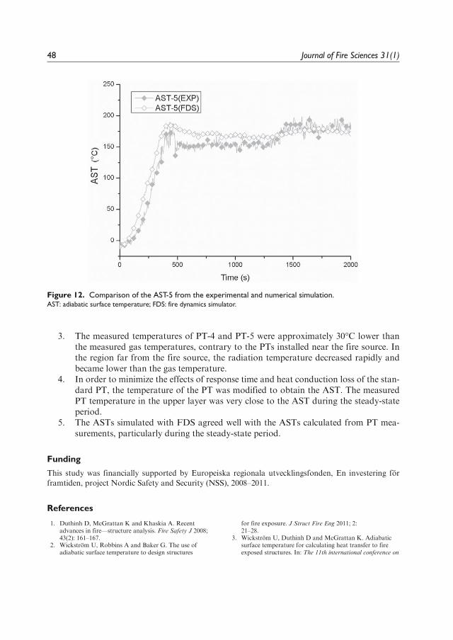
3. The measured temperatures of PT-4 and PT-5 were approximately 30�C lower thanthe measured gas temperatures, contrary to the PTs installed near the fire source. Inthe region far from the fire source, the radiation temperature decreased rapidly andbecame lower than the gas temperature.

4. In order to minimize the effects of response time and heat conduction loss of the stan-dard PT, the temperature of the PT was modified to obtain the AST. The measuredPT temperature in the upper layer was very close to the AST during the steady-stateperiod.

5. The ASTs simulated with FDS agreed well with the ASTs calculated from PT mea-surements, particularly during the steady-state period.

Funding

This study was financially supported by Europeiska regionala utvecklingsfonden, En investering forframtiden, project Nordic Safety and Security (NSS), 2008–2011.

References

1. Duthinh D, McGrattan K and Khaskia A. Recentadvances in fire—structure analysis. Fire Safety J 2008;43(2): 161–167.

2. Wickstrom U, Robbins A and Baker G. The use ofadiabatic surface temperature to design structures

for fire exposure. J Struct Fire Eng 2011; 2:21–28.

3. Wickstrom U, Duthinh D and McGrattan K. Adiabaticsurface temperature for calculating heat transfer to fireexposed structures. In: The 11th international conference on

Figure 12. Comparison of the AST-5 from the experimental and numerical simulation.AST: adiabatic surface temperature; FDS: fire dynamics simulator.


fire science and engineering, Interflam ’07, London, UK,3–5 September 2007.

4. Wickstrom U. The plate thermometer—a simpleinstrument for reaching harmonized fire resistance tests.Fire Technol 1994; 30(2): 195–208.

5. McGrattan K, McDermott R, Hostikka S, et al. Firedynamics simulator (version 5)—user’s guide. 2010. NISTSpecial Publication 1019-5. Washington: US GovernmentPrinting Office.

6. Ingason H and Wickstrom U. Measuring incident radiantheat flux using the plate thermometer. Fire Safety J 2007;42(2): 161–166.

7. Wickstrom U. Adiabatic surface temperature and the platethermometer for calculating heat transfer and controllingfire resistance furnaces. In: The 9th internationalsymposium on fire safety science, Beijing, China, 21–26September 2008.

8. Wickstrom U, Jansson R and Tuovinen H. Validation firetests on using the adiabatic surface temperature for

predicting heat transfer. SP Report 2009:19, 2009. Boras:SP Technical Research Institute of Sweden.

9. Wickstrom U. The adiabatic surface temperature and theplate thermometer. In: The 10th international symposiumon fire safety science, Maryland, USA, June 19–24 2011,pp. 1001–1011.

10. Bystrom A, Cheng XD, Wickstrom U, et al.Full-scaleexperimental and numerical studies on compartment fireunder low ambient temperature. Build Environ 2012; 51:255–262.

11. Haggkvist A. The plate thermometer as a mean ofcalculating incident heat radiation—a practical andtheoretical study. Master’s Thesis, Lulea University ofTechnology, Lulea, Sweden, 2009.

12. Quintiere JG. Fundamentals of fire phenomena. Chichester:John Wiley & Sons Ltd, 2006.

13. Hietaniemi J and Mikkola E. Design fires for fire safetyengineering. VTT working papers 139, 2010.

Appendix 1

Nomenclature

hc Convective heat transfer coefficient (W/m2 K)hASTc Convective heat transfer coefficient of adiabatic

surface (W/m2 K)hPTc Convective heat transfer coefficient of plate

thermometer (PT) (W/m2 K)hr Radiative heat transfer coefficient (W/m2 K)hASTr Radiative heat transfer coefficient of adiabatic

surface (W/m2 K)hPTr Radiative heat transfer coefficient of PT (W/m2 K)_q00con Convection heat flux at the surface (W/m2)_q00inc Incident heat flux at the surface (W/m2)_q00rad Radiation heat flux at the surface (W/m2)_q00tot Total heat flux at the surface (W/m2)C Heat capacity of PT (J/m2 K)K Heat conduction coefficient of PT (W/m2 K)Tg Temperature of hot gas (�C or K)Tr Blackbody radiation temperature (�C or K)Ts Surface temperature (�C or K)TAST Adiabatic surface temperature (�C or K)TPT Measured temperature of PT (�C or K)e Emissivity (—)s Stefan–Boltzmann constant (W/m2 K4)

Author biographies

Alexandra Bystrom is a Phd student in Lulea University of Technology. Her research area includesstructure behavior in fire and heat transfer in fire engineering.

Xudong Cheng is a Associate Professor in University of Science and Technology of China. His researcharea includes compartment fire, fire risk evaluation and structure behavior in fire.

Bystrom et al. 49

Ulf Wickstrom is a Professor in SP Technical Research Institute of Sweden and Lulea University ofTechnology. His research area mainly focuses on heat transfer in fire engineering.

Milan Veljkovic is a Professor in Lulea University of Technology. His research area mainly includessteel structures, structure behavior in fire and steel tower for wind turbines.


Paper A3

Large Scale Test on a Steel Column Exposed to

Localized Fire

by Alexandra Byström, Johan Sjöström, Ulf Wickström,

David Lange, Milan Veljkovic

Journal of Structural Fire Engineering

Volume 5 · Number 2 · 2014

147

Large Scale Test on a Steel Column Exposed toLocalized Fire

Alexandra Byströma*, Johan Sjöströmb*, Ulf Wickströma,b, David Langeb and Milan Veljkovicb

aLuleå University of Technology, LTU, Swedene-mails: [email protected], [email protected].

bTechnical Research Institute of Sweden, SPe-mails: [email protected], [email protected], [email protected]

AbstractA localized fire is a fire which in a compartment is unlikely to reach flash-over anduniform temperature distribution. Designing for localized fires is generally more difficultthan for flash-over compartment fires because of the complexity of the problem. There isalso a lack of experimental data. We report here on a full scale test series on a steelcolumn exposed to localized fires. The setup is a 6 meters tall hollow circular column, f = 200 mm with a steel thickness of 10 mm. The unloaded column was hanging centrallyabove different pool fires. Temperatures of gas and steel were measured bythermocouples, and adiabatic surface temperatures at the steel surface were measured byplate thermometers of various designs. The results are compared with estimates based onEurocode 1991-1-2 which in all cases studied overestimate the thermal impact for thissetup. The input from plate thermometers was used to compute the steel temperaturesusing finite element methods. Excellent agreement was found if the radiation exchangewithin the column due to asymmetry of the exposure was taken into account.

Keywords: Localized fire, Plate thermometer, steel column, adiabatic surfacetemperature, TASEF.

ABBREVIATIONSA Surface area of the member which is exposed per unit length, [m2]C Correction factor for thermal storage, [J/m2K]D Diameter oft he burning source, [m]d Flame thickness, [m]DHc Heat of combustion for the evaporated gases, [J/kg]hc Convective heat transfer coefficient, [W/m2K]hr Radiative heat transfer coefficient, [W/m2K]K Correction factor for conductive losses, [W/m2K]k Absorption coefficient of radiant heat in the flame, [m-1]Lf Height of flame, [m]m. Mass burning rate, [kg/s]Q.

Heat release rate, [W]Q.

c Convective part of energy release rate, [W]q.�� Heat flux, [W/m2]T Temperature, [K]t Time, [s]ta Fire growth rate coefficient or time specified to reach Q

., = 1MW, [s]

V Volume of the member per unit length, [m3]z Height of the flame, [m]z0 Height of virtual origin of the flame, [m]

* These authors contributed equally to this work

148 Large Scale Test on a Steel Column Exposed to Localized Fire


Greeke Emissivity, [-]r Density, [kg/m3]s Stefan-Boltzmann constant, [s = 5.67·10-8 kg/ s3K4]c Combustion efficiency, [-]

Subscriptsabs AbsorbedAST Adiabatic Surface Temperaturecon Convectionemi Emittedfl Flameg Gasinc Incidentnet NetPT Plate Thermometerr Radiations Surface

1. INTRODUCTIONIn large enclosures like air terminals a fully developed fire with high uniform temperatures is unlikelyto occur. Still, an intense fire could locally expose structures to severe thermal conditions although themean temperature in the enclosure remains low. Usually structures are designed to resist the standardfire according to EN 1363-1 for a specified time. Alternatively, parametric fires as specified in theEurocode (EN 1991-1-2 - Annex A) could be applied but all these design fires are intended forrelatively small spaces where flashover with high and uniform temperatures can develop. We may forlarge enclosures instead assume localized fires, as specified in EN 1991-1-2 - Annex C, when designingstructures. The fire exposure then depends on the fuel and the dimensions of the flames. Often onlyparts of a structural element will be subjected to severe exposure which may influence the load-bearingcapacity in comparison to a uniform exposure. Asymmetric fires may make the exposure on slendercolumns more severe. More detailed analyses allow for taking into account better resolvedtemperatures which include variations along a structures length or its height.

Very little experimental data from full scale localised fire tests is available in the literature. Thiswork summarizes full-scale experiments on a steel column exposed to pool fires from heptane anddiesel in a large room. All the experimental data can be downloaded from the SP website [1]. For designpurposes, temperatures resulting from localized fires can be determined from plume theories [2, 3],such as that which has been implemented in the models of Eurocode 1.

2. BACKGROUNDThe heat transfer from the flame and hot gases to a surface consists of three independent components,absorbed radiation, emitted radiation and convective heat transfer. A surface absorbs a portion(depending on the surface emissivity/absorptivity) of the incident radiant flux against the surface, q

. ��abs.

Irrespective of the incident radiation, the surface also emits heat, q.��emi, proportional to the fourth power

of the surface temperature. Thus, the total heat flux at the surface, q.��to-t, also accounting for convective

heat flux, q. ��con, is given by:

q.��tot = q

. ��abs - q

.��emi + q

. ��con (1)

Normally in fire safety engineering surface emissivities are taken to be wavelength independent, andconvective heat transfer is assumed to be linearly proportional to the difference between the surface-and gas temperatures. When flames are adjacent to a structure the gas temperature is assumed to be

equal to the flame temperature Tfl. The total heat transfer to a surface exposed to a localized fire cantherefore be expressed as:

(2)

where the incident heat flux, .

(3)

where es is surface emissivity, efl is flame emissivity, s; is the Stefan-Boltzmann constant, Tfl and Ts arethe temperatures of flame and surface, respectively, and hc is the convective heat transfer coefficient.The flame emissivity, efl, is given by efl = 1 - exp(-kd), where d is flame thickness and k absorptioncoefficient of radiant heat in the flame. In Eq. 3 any radiation except directly from the flames isassumed negligible.

2.1. Basic Theory of ASTThe adiabatic surface temperature (AST) is defined as the temperature of a solid surface which doesnot gain or lose any heat by conduction. It can be obtained by solving eqn (4) (see Ref. [4]):

(4)

where Tg is the adjacent gas temperature.AST is a measure of the thermal exposure level which depends on the surface emissivity and

convective heat transfer coefficient. Knowing the AST enables one to calculate the heat transfer to asurface with only one effective fire temperature as given by the equation [5]:

(5)

Thus, measuring AST would give us sufficient information of the heat transfer without the detailedknowledge specified above. Measuring AST exactly is hard but a close approximation is achieved withthe use of plate thermometers (PT), originally invented to measure and control temperature in fireresistance furnaces. The PT is insulated (low losses to backside), large (convective heat transfer similar tostructural surfaces) and has one exposed side (it “sees” the same thing as a structural surface). Figure 1ashows a standard plate thermometer according to ISO 834. It is made of a shielded thermocouple weldedto the centre of a 0.7 mm thick metal plate which is insulated on its back side. The exposed front face is100 mm by 100 mm. On the back side of the metal plate there is a 10 mm thick insulation pad. For thisexperiment some of the PT had a curved surface and were embedded into the column surface, see Ref. [1]or Figure 1b below.

The temperature measured by PT is close to the AST. However, there are some differences betweenthem due to the response time and the heat conduction loss of the PT. The correction that is requiredhas been analysed both experimentally and through finite element analysis [5]. The heat balance at theexposed surface of a PT may be written as:

(6)

where the correction factor for conductive losses and thermal storage are K = 8 W/m2K and C = 4200J/m2K, respectively [5]. TPT is the temperature of the PT exposed surface.

� ε ( ) ( )′′ = − + −q T T h T Ttot s AST s c g AST4 4

�ε ε σ ( )= ′′ − + −q T h T T0 s inc s AST c g AST4

� ε σ ε( ) ( )′′ = − + −q T T h T Ttot s fl fl s c fl s4 4

ε σ′′ =q Tinc fl fl4�

� �ε ε σ ( )′′ = ′′ − + −q q T h T Ttot s inc s s c fl s4

�ε σ( ) ( ) ( )′′ − + − − − =q T h T T K T T CdT

dtPT inc PT c g PT g PTPT4

Alexandra Byström, Johan Sjöström, Ulf Wickström, David Lange and Milan Veljkovic 149


Combining eqns (4 and 6) allows us to calculate TAST from a series of consecutive PT measurementsby an iterative procedure presented in [6, 7]

(7)

2.2. Thermal action, according to the EN 1991-1-2According to the EN 1991-1-2 a localized fire is a design fire where flash-over is unlikely to occur andwhich involves only a limited area of the fire load of the compartment. Here we summarise thecalculation method of the thermal exposure from a localised fire as defined in the Eurocode 1. Theflame is defined through the Heskestad plume equations [2]. The height of flames is determined fromthe burning source size and heat release rate through the equation

, (8)

where D (m) is the burning source diameter and Q.(W) the heat release rate. The latter, according to the EN

1991-1-2, is time dependent with a t2-dependence such that it fits the time specified to reach Q = 1 MW.

(9)

ε σ

( )

( ) ( )

= +

⎡⎣⎢

⎤⎦⎥

− −

+

= + −

− −

−T TC

dT

dtK T T

h h

h T T T T

,

where

ASTi

PTi

PT

i

ASTi

PTi

ri

c

ri

PT ASTi

PTi

ASTi

PTi

1 1

1

2 2

�= − +L D Q1.02 0.0148f2 5

=⎛

⎝⎜

⎞

⎠⎟

α

Qt

t10

.6

2



a) The standard plate thermometer according to ISO 834 and EN 1363-1.

b) Special PT designed to be embedded at the surface of the circular column.

Figure 1. Two designs of plate thermometers used in the experiments.

For this study, we instead calculate the heat release rate based on the mass burning rate (taken fromthe experiments), the heat of combustion for the evaporated gases, DHc and the combustion efficiency,c using the following relation:

(10)

where DHc is taken from references [8, 9].When the flame is not impacting the ceiling of a compartment or in case of fire in open space, the

temperature T(z)[°C] in the plume along the symmetrical vertical flame axis at height z [m] is given by:

(11)

(12)

where z0 is the virtual origin and Qc = 0.8Q [W]. D is diameter of the burning source.There is no equation in the Eurocode for T(z) > 900. We therefore assume that the flame temperature

is constant at heights lower than the upper limit of eqn (11).On the fire exposed surfaces the net heat flux per unit surface area is determined according to the

Eurocode as:

(13)

where Tr is the effective radiation temperature of the fire environment efl should be set

to 1, es to 0.8 and hc to 25 W/m2K unless more detailed values are vailable. In our case, theconfiguration/view factor, F, can be set to unity. For an engulfing flame Tr can be set to the gastemperature.

Eqn (13) is different from eqn (3) in that both the flame emissivity and view factor are included forthe emitted radiation. The flame emissivity and the view factor are, however, irrelevant for the radiationemitted from the surface. For thick sooty flames, where the emissivity is close to one, completelyengulfing the structure, it makes a marginal difference. However, for cleaner fuels, like methanol, orfor a fire not directly adjacent to the structure, the equation of the Eurocode is not correct.

We use a one-dimensional model for calculating the steel temperature, assuming lumped heatcapacitance. The final expression for the steel/surface temperature increase at time step i, calculatedwith a time step of Dt, can, according to EN 1991-1-2, be expressed as:

(14)

where r is density, c specific heat, A is the surface area of the member which is exposed per unit length,and V is the volume of the member per unit length.

In the present study two scenarios of high and low thermal exposure are analysed. The high exposurescenario is for a complete combustion (c = 1 in eqn (10)) and fully radiant gas at heights above theflame height. The low exposure scenario is defined using c = 1 and no radiation to the structure abovethe flame height. The method described in the Eurocode for calculating plume temperatures will beused to evaluate the thermal exposure to a column for the range of scenarios.

2.3. Previous WorkThere are some experimental data from full scale fires available in the literature, such as the Murcia firetests conducted in the large scale atrium with heptane pools of two diameters [10]. The study presentsmeasurements of gas and wall temperature as well as airflow at the inlets during fire in the large scaleatrium. Limited experimental data on structural elements exposed to localized fires are available, such

ρ= +

Δ+T T

q AV t

csi

si net

i

1

q ,inc4 � σ( )≡ ′′

� φε ε σ ( ) ( )′′ = − + −q T T h T Tnet s fl r s c g s4 4

� χ= ΔQ m Hc

.

T z Q z z20 0.25 900,c2 3

0

5 3�( ) ( )= + − ≤−

�= − +z D Q1.02 0.0052402 5



as unprotected ceiling slab [11, 12] and a 2 meter unprotected steel column [13]. Steel temperatures andheat flux were measured for further analysis and correlation between experiment and simulations wasperformed.

A series of tests on a steel beam in a Room Corner test room (according to ISO 9705) was conductedat SP [14]. The beam was hanging 20 cm from the ceiling and a gas burner was placed in the cornerand under the beam. The result shows a very large difference in the temperatures probed by smallthermocouples and plate thermometers. The PTs are much less sensitive to convection as they have alower convective heat transfer coefficient relative the small thermocouples and will therefore adjust totemperatures dependent on the incident radiation to the specimen surface.

A similar concept to the localised fire is the travelling fire where a fire is moving over the floor plate,burning only a limited are at one time. A design methodology has been developed for those types offires and further work is on-going [15].

This work summarizes full-scale experiments on a steel column exposed to various pool fires in alarge room. All the experimental data can be downloaded from the SP website [1]. Heat release rate hasbeen calculated according to the theories described in [8, 9].

3. TEST PROCEDUREThe experiments were carried out in the large fire hall of SP, approximatively 20 m by 20 m, and 20 mhigh. A full size (6 m tall, 200 mm wide and 10 mm thick) circular, unprotected and unloaded steelcolumn was exposed to circular pool fires with various burning area. Its interior was empty. The columnwas hanging centrally, 20 cm over the fuel container in the middle of the fire hall under the mainexhaust hood. The lower and upper ends of the column were sealed and the column was fixed at theupper end.

To aid in discussion four positions are defined on the columns cross section, Figure 2. Thesenumbered positions are used to describe where different measurements were taken. At one position/side(see Figure 2) of the column (position 1) gas temperatures, steel temperatures and plate thermometer(PT) temperatures were measured at heights of 1, 2, 3, 4 and 5 meters along the column. Thus, theinstruments at e.g. 2 meters along the column are situated 2.2 meters above the fuel surface. Gastemperatures were measured using welded 0.25 mm thermocouples. Steel temperatures were measuredwith thermocouples fixed about 1 mm into the steel structures. The plate thermometers were standardplate thermometers as used in furnace testing according to EN 1363-1 but mounted only a few cm fromthe steel surface. In two positions, ±90º from position 1, curved PTs were mounted inside the steelcolumn on height 2 and 4 together with gas thermocouples, see figure 3. Opposite to position 1 gas andsteel temperatures were measured together with PTs at 2 and 4 meters height.

Three experiments were performed. Diesel and heptane were burned using a pool diameter of 1.1 m.An additional diesel fire was also run with a pool diameter of 1.9 m. The fuel container was placed ona balance to measure the mass loss rate. Two meters from the column was a vertical stone woolinsulation board, 6 m high and 1.2 m wide to protect instrumentation anchors and data collection.Further details on the experimental setup can be found in Ref. [1].

Table 1 shows the calculated fuel characteristics needed for calculations according to the Eurocodedescribed above.

4. RESULTS AND DISCUSSIONS4.1. Results from the ExperimentsFigure 4 shows a series of pictures from the smaller diesel fire of diameter 1.1 m. The flames were tiltedtowards position 1 of the column cross section due to uneven natural flow of air into the room. Theywere flickering to heights between 2 m and 3.5 m, and above 1 m the flame is preferentially leaning inthe direction of position 1.

By increasing the pool diameter to 1.9 m, the size of the flames increased considerably. The heightwas then constantly over 4 m, sometimes reaching well over 5 m. A movie of the larger fire can beviewed on SP’s web page [1]. Selected temperatures along the position 1 direction are presented in



Figure 5. It is quite evident that the small 0.25 mm TCs and the PTs display essentially the sametemperatures in this position. This is not the case for other positions, e.g. at position 2 at 4 metersheight, the PT temperature exceeds the gas temperature. All measured data can be downloaded fromRef. [1].

As the flame tilted towards position 1, the thermal exposure was also asymmetric which was clearlyindicated by the PTs. Figure 6 shows PT measurements around the column at 2 and 4 metres anddisplays a difference between positions 1, 2 and positions 3, 4 of 200 ºC. The asymmetry has naturalconsequences on the steel temperatures. From the movie [1] one can observe the curvature of thecolumn due to uneven thermal expansion.

The recorded steel temperatures for the larger diesel fire (Ø = 1.9 m) are shown in figure 7. Figure 8 and figure 9 show the equivalent temperatures for the smaller diesel fire (Ø = 1.1 m) and the



Insulation for instrumentationdistance = 2m

Pos 2{embedded PT,gas, steel}@ 2 & 4 m

Pos 1{PT, gas, steel}@ 1,2,3,4,5 m

Pos 4{embedded PT,gas, steel}@ 2 & 4 m

Pos 3{PT, gas, steel}@ 2 & 4 m

4 m

3 m

~6

m

2 m

1 m

5 m

Figure 2. Left: experimental setup seen from position 1. The grey squares indicate platethermometers. Right: cross section of the column from top view showing the differentinstrumentations in the different positions.

Figure 3. Thermocouples and PT setup.

Table 1. Fuel characteristics, mass loss rate, heat of combustion (DHc), Heat release rate(HRR) and flame height. HRR and flame height is calculated based on 70 % combustion

efficiency.

Fuel Mass loss rate DHc [8, 9], HRR (MW), Flame height (m), (kg/s) (MJ/kg) eqn. (10) eqn. (8)

Heptane 0.051 44.6 1.6 3.3Diesel, diameter 1.1 m 0.032 44.4 1 2.6Diesel, diameter 1.9 m 0.107 44.4 3.3 4.1

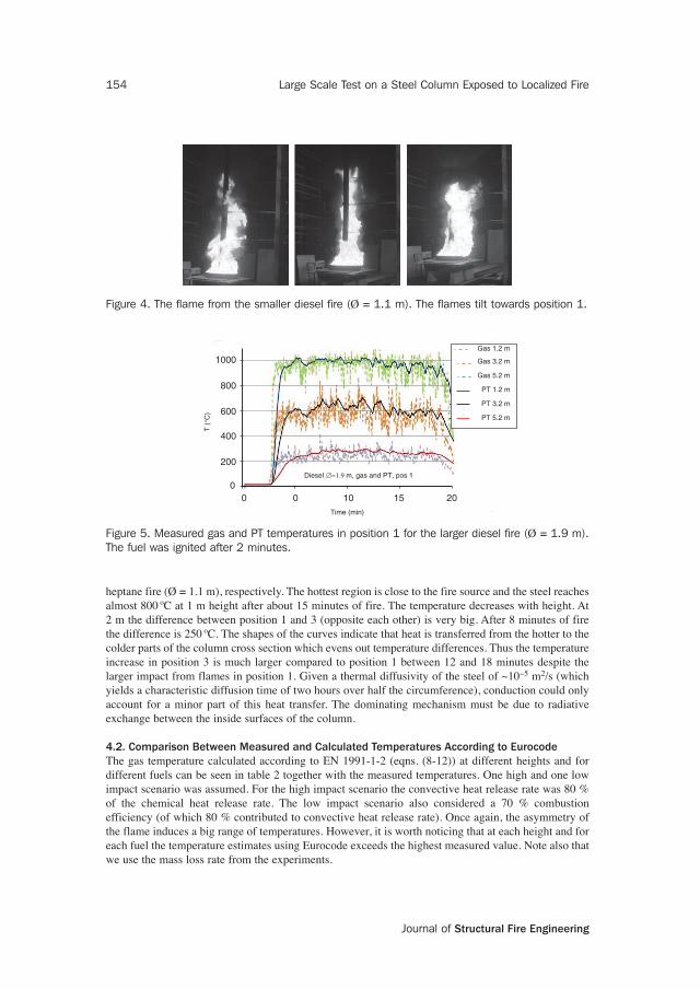
heptane fire (Ø = 1.1 m), respectively. The hottest region is close to the fire source and the steel reachesalmost 800 ºC at 1 m height after about 15 minutes of fire. The temperature decreases with height. At2 m the difference between position 1 and 3 (opposite each other) is very big. After 8 minutes of firethe difference is 250 ºC. The shapes of the curves indicate that heat is transferred from the hotter to thecolder parts of the column cross section which evens out temperature differences. Thus the temperatureincrease in position 3 is much larger compared to position 1 between 12 and 18 minutes despite thelarger impact from flames in position 1. Given a thermal diffusivity of the steel of ~10-5 m2/s (whichyields a characteristic diffusion time of two hours over half the circumference), conduction could onlyaccount for a minor part of this heat transfer. The dominating mechanism must be due to radiativeexchange between the inside surfaces of the column.

4.2. Comparison Between Measured and Calculated Temperatures According to EurocodeThe gas temperature calculated according to EN 1991-1-2 (eqns. (8-12)) at different heights and fordifferent fuels can be seen in table 2 together with the measured temperatures. One high and one lowimpact scenario was assumed. For the high impact scenario the convective heat release rate was 80 %of the chemical heat release rate. The low impact scenario also considered a 70 % combustionefficiency (of which 80 % contributed to convective heat release rate). Once again, the asymmetry ofthe flame induces a big range of temperatures. However, it is worth noticing that at each height and foreach fuel the temperature estimates using Eurocode exceeds the highest measured value. Note also thatwe use the mass loss rate from the experiments.



Figure 4. The flame from the smaller diesel fire (Ø = 1.1 m). The flames tilt towards position 1.

1000

800

600

400

200

00

0 10 15 20

Gas 1.2 m

Gas 3.2 m

Gas 5.2 m

PT 1.2 m

PT 3.2 m

PT 5.2 m

T (

°C)

Time (min)

Diesel ∅=1.9 m, gas and PT, pos 1

Figure 5. Measured gas and PT temperatures in position 1 for the larger diesel fire (Ø = 1.9 m).The fuel was ignited after 2 minutes.

The temperatures when calculated using the Eurocode method yields significant differences in steeltemperatures when compared against the measured values. The Eurocode temperature estimations werewithout exception higher than the measured, even when we compared the estimations to the side of the



800

600

400

200

1000

2m p1

2m p2

2m p4

2m p3

4m p3

4m p4

Diesel 1.9 m, PT

Time (min)

T (°

C)

4m p1

4m p2

0151050 20

Figure 6. Left: PT temperatures at 2.2 and 4.2 m height in all positions for the larger diesel fire(Ø = 1.9 m). “2m p4” indicate 2 meters height at position 4. Right: a photo of the same fire with>4 m flames and a characteristic asymmetry.

700

600

500

400

300

200

100

800Diesel 1.9 m

Time (min)

1 m pos 1

2 m pos 1

2 m pos 3

3 m pos 1

4 m pos 1

4 m pos 35 m pos 1

0151050 20

T (

°C)

Figure 7. Measured steel temperatures for the larger diesel fire (Ø = 1.9 m). Solid and dashedlines represent position 1 and 3, respectively. The fuel was ignited at 2 minutes.

700

600

500

400

300

200

100

800

0

T (

°C)

20151050 25Time (min)

Diesel 1.1 m1 m pos 1

2 m pos 1

2 m pos 3

3 m pos 14 m pos 14 m pos 35 m pos 1

Figure 8. Measured steel temperatures for the smaller diesel fire (Ø = 1.1 m). Solid and dashedlines represent position 1 and 3, respectively.



700

600

500

400

300

200

100

800

0

T (

°C)

20151050 25Time (min)

Heptane 1.1 m

1 m pos 1

2 m pos 1

2 m pos 3

3 m pos 1

4 m pos 14 m pos 35 m pos 1

Figure 9. Measured steel temperatures for the heptane fire (Ø = 1.1 m). Solid and dashed linesrepresent position 1 and 3, respectively.

Table 2. Temperatures after 10 minutes from ignition

HeightFuel and pan above fuel Tgas, measured Tgas calculated Tsteel, measured Tsteel calculateddiameter surface (m) (°C)1 Eurocode (°C) (°C) Eurocode (°C)Heptane, 1.2 900 900 584 747diameter 1.1 m 2.2 300-650 900 265-457 747

3.2 500 661-883 214 514-7064.2 150-280 353-442 76-122 204-2805.2 180 260-325 63 97-183

Diesel, 1.2 800 900 495 747diameter 1.1 m 2.2 250-500 720-900 175-281 583-747

3.2 250 363-455 96 212-2924.2 110-150 212-263 54-65 82-1415.2 120 162-200 44 66-104

Diesel, 1.2 950 900 711 747diameter 1.9 m 2.2 480-800 900 415-660 747

3.2 640 825-900 363 699-7474.2 220-400 464-583 144-261 301-4265.2 250 347-435 118 200-248

1 The measured gas temperatures are from position 1 if only one number is given. At heights where temperatures were measuredaround the column values are given in intervals.2 The Eurocode calculations are given as intervals between the high and low impact scenario.

column which was most severely exposed (position 1). Figure 10 shows the comparison of themeasured steel temperatures and the temperatures calculated according to the EN 1991-1-2 [16].

4.3. Finite element analysis based on PT measurementsTo calculate the steel temperatures from the results of PT measurements we used the finite element codeTASEF. At 2 and 4 metres along the column the AST for all four positions around the column iscalculated based on the PT measurements according to eqn (7). The heat transfer is thereafter evaluatedbased on a thermal boundary condition given by eqn (5). The column is approximated to a squaresection of 200 mm by 200 mm which is deemed reasonable as the influence of the tangential heat fluxby conduction in the steel is negligible in comparison to the heat flux from the fire. The materialproperties of steel were defined according to Eurocode 3. The convective heat transfer coefficientbetween the external gas and the steel was chosen to be 25 W/m2K on the outer surfaces. Heat transfer



by radiation was calculated assuming emissivity equal to 0.9 for both external and internal surfaces.Internal heat exchange in the steel section is assumed to occur by radiation and convection. The heatexchange by radiation between each of the internal steel element surfaces was then calculated. The convective heat transfer was calculated by first calculating the internal gas temperature as aweighted average temperature of the surrounding node temperatures. The heat transfer between theinternal gas and the steel surfaces was then calculated assuming a convective heat transfer coefficientequal to 1 W/m2K. Figure 11 shows the mesh structure and the thermal boundary condition on one sideof the section.

Using the PT and gas temperature readout, the AST can be calculated according to eqn. (7). Thesevalues are thereafter used as input to finite element simulations for the Ø = 1.9 m diesel fire at 2 and 4 meters along the column. Note that individual AST are calculated for each of the four positions aroundthe column periphery. AST is used as the effective fire temperature according to eqn. (4). Radiation and

700600500400300200100

800900

2 min

4

6

10

14

0

4321 5 6

Ste

el T

(°C

)Experimental

Heptane D=1.1 m

Height above fuel (m)

700600500400300200100

800900

2 min

4

6

10

14

0

4321 5 6

Ste

el T

(°C

)

EurocodeHeptane D=1.1 m


700600500400300200100

800900

2 min

4

6

10

14

0

4321 5 6

Ste

el T

(°C

)

ExperimentalDiesel D=1.1 m


700600500400300200100

800900

2 min

4

6

10

14

0

4321 5

Ste

el T

(°C

)

EurocodeDiesel D=1.1m


700600500400300200100

800900

2 min

4

6

10

14

0

4321 5 6

Ste

el T

(°C

)

ExperimentalDiesel D=1.9 m


700600500400300200100

800900

2 min

4

6

10

14

0

4321 5 6

Ste

el T

(°C

)

EurocodeDiesel D=1.9 m


Figure 10. Measured steel temperatures (left) and calculated steel temperature according to theEN 1991-1-2 (right) for the three different fires. The legends show time from ignition. The errorbars represent the spread in measured around the periphery for experimental data and the spreadbetween the high and low impact scenario for Eurocode data.


10 mm

157 mm

)(4.,

'', tTq iposASTradinc σ=�

( )siiposASTcconv TtThq −= )(.,''�

4''sisemi Tq σε=�

∑= 4''sisiinc TAq σε�

( )siinnergasinnercconv TThq −= ,,''�

4''sisemi Tq σε=�

Figure 11. Mesh distribution and thermal boundary conditions for the FEM simulations.

0

50

100

150

200

250

300

350

0 10 20

T(°

C)

Time (min)

4 m along the column

Steel (exp), p1

Steel (FEM), p1

Steel (exp), p3

Steel (FEM), p3

0

100

200

300

400

500

600

700

800

0 5 10 15 20

T(°

C)

Time (min)

2 m along the column

Steel (exp), p1

Steel (FEM), p1

Steel (exp), p3

Steel (FEM), p3

Figure 12. Steel temperatures of the column in position 1 and 3 as measured (dotted and dashedlines) and as obtained from the finite element simulation using eqn. (5) as boundary condition(solid lines). Left: 2 m along the column. Right: 4 m along the column.

convection exchange was taken into account between the inner surfaces of the steel section. Thecalculated steel temperatures and corresponding measured temperatures are found in figure 12.

The measured and simulated values match very well despite the unstable and inhomogeneous natureof the flame. This suggests that PT measurements yield very valuable data for expressing the intensityof thermal exposure (to a structure of similar emissivity) as was earlier shown for a beam [1][14].

5. CONCLUSIONSThis study gives unique reference data on steel, gas and PT temperatures for a full scale columnexposed to localized fires. The fires studied were two different sized diesel pool fires (Ø = 1.1 and 1.9m) and one heptane pool fire (Ø = 1.1 m). The data is available for downloading on the SP website [1].

In the test reported here, large parts of the column were at times engulfed in flames only on one side,introducing a temperature difference of up to 250ºC around the column periphery. This reduces the


temperature but may in practice have harmful effects on the load-bearing capacity of a column as itinduces a curvature of the column the thereby eccentric loading. The mechanical effects on a loadedbeam for these asymmetric exposure is investigated in [17].

The method described in Eurocode 1 for calculating plume temperatures and heat transfer to thecolumn gives conservative results for gas and steel temperatures when compared with the results of theexperiment, as expected.

This study also shows that the plate thermometer PT readouts, transformed to adiabatic surfacetemperature AST can be used to accurately calculate the temperature of the steel structure. In the casestudied here it is imperative to consider the internal cross section heat exchange by radiation andconvection as the column was asymmetrically fire exposed.

ACKNOWLEDGEMENTSThe authors gratefully acknowledge the financial support provided by The Swedish fire research board,Brandforsk, Sweden. B. Bogren and L. Gustavsson are also acknowledged for their valuable assistancecaring out the fire tests.

REFERENCES[1] http://www.sp.se/en/index/services/localized_fire/Sidor/default.aspx

[2] Heskestad, G., Fire Plumes, Flame height and Air entrainment, SFPE Handbook of FireProtection Engineering, 3nd edition, National Fire Protection Association, Quincy, MA 2002.

[3] McCaffrey, B.J., Purely Buoyant Diffusion Flames: Some Experimantal Results, Fire SafetyJournal, vol 3, pp 107–121, 1980.

[4] Wickström U, Duthinh D, McGrattan K., Adiabatic surface temperature for calculating heattransfer to fire exposed structures, The 11th International Conference on Fire Science andEngineering Interflam, Sept. 2007, 3–5.

[5] Häggkvist A, Sjöström J, Wickström U., Using plate thermometer measurements to calculateincident heat radiation, Journal of Fire Sciences.

[6] Byström A., Cheng X., Wickström U., Veljkovic M., Measurement and calculation of adiabaticsurface temperature in a full-scale compartment fire, Journal of Fire Sciences. 31 (2013), 35–50.

[7] Wickström U, Robbins A, Baker G., The use of adiabatic surface temperature to design structuresfor fire exposure, Journal of structural fire engineering, 2(2011), 21–28.

[8] Babrauskas V., Heat release rate, SFPE Handbook of Fire Protection Engineering, 3rd edition,National Fire Protection Association, Quincy, MA 2002.

[9] Karlsson B.,Quintiere J.G., Enclosure fire dynamics, CRC Press, Boca Raton, FL, 2000.

[10] Gutierrez-Montes C., Sanmiguel-Rojas E., Vied,a A., Rein G., Experimental data and numericalmodeling of 1.3 and 2.3 MW fires in a 20 m cubic atrium, Building and Environment, Vol: 44, i:9, pp 1827-1839.

[11] Hasemi Y., Yokobayashi Y., Wakamatsu T., Ptchelintsev A.V., Modeling of the heat mechanismand thermal response of structural components exposed to localized fires: A new application ofdiffusion flame modeling to fire safety engineering, 13th meeting of the UJNR panel of fireresearch and safety, Vol 1, March, 1996.

[12] Wakamatsu T., Hasemi Y., Ptchelintsev A.V., Heating mechanism of building componentsexposed to a localized fire. CFD prediction to a localized fire, Fire science & technology, Vol 20,No1, 2000.

[13] Li G.-Q., Zhang C., Thermal response of steel columns exposed to localized fires – numericalsolutions and comparison with experimental results, Journal of Structural fire engineering, Vol 2,No 4, 2011.

[14] Jansson R., Wickström U., Tuovinen H.,Validation fire tests on using the adiabatic surfacetemperature for predicting heat transfer, SP Report 2009:19.



[15] J Stern-Gottfried, G Rein, Travelling Fires for Structural Design. Part II: Design Methodology,Fire Safety Journal 54, pp. 96–112, 2012

[16] Franssen J.M. and Real P.V., Fire Design of Steel Structures, 1st edition, Ernst & Sohn, Berlin,2010, 17–45.

[17] Lange D., Sjöström J., Mechanical response of a partially restrained column exposed to localizedfires, Fire Safety Journal, 2014, DOI 10.1016/j.firesaf.2014.05.013.



Paper B1

Thermal analysis of a pool fire test in a steel

container

by Xudong Cheng, Alexandra Byström, Ulf Wickström,

Milan Veljkovic

Journal of Fire Science

Article

Journal of Fire Sciences

30(2) 170–184

� The Author(s) 2012

Reprints and permissions:

sagepub.co.uk/journalsPermissions.nav

DOI: 10.1177/0734904111432834

jfs.sagepub.com

Thermal analysis of a pool firetest in a steel container

Xudong Cheng1,2, Alexandra Bystrom1, Ulf Wickstrom1,3

and Milan Veljkovic1

Date received: 18 October 2011

AbstractA pool fire test was conducted in an uninsulated steel container under low ambient temperaturecondition, at 220�C. The heat balance of the enclosure fire was analyzed. The size of the con-tainer was 12 m3 2.4 m and 2.4 m high, and it was made of 3-mm-thick steel. During the fire test,the fuel mass loss rate was recorded and the temperatures at different positions were measuredwith high-temperature thermocouples and plate thermometers. The fire scenario was simulatedby using fire dynamics simulator software, and the simulated and measured results were com-pared. The coarse high-temperature thermocouple responded slower, and therefore, tempera-ture measured by the high-temperature thermocouple was corrected to eliminate the effect ofthe thermal inertia. Furthermore, a simple two-zone model was proposed for estimating gas tem-perature in the enclosure of the highly conductive steel walls assuming a constant combustionrate. The convective and radiative heat transfer resistances at the inside and outside surfaces ofthe enclosure were analyzed.

KeywordsThermal analysis, adiabatic surface temperature, pool fire, FDS

Introduction

Liquid pool fires are regarded as suitable fire sources for investigating the features of fires intunnels and other enclosures as well as for studying water mist suppression.1–3 The combus-tion characteristics of liquid pool fires have been studied in detail during the past decades.Thus, the experiments carried out by Blinov and Khudiakov4 showed that the burning rate

1Division of Structural and Construction Engineering, Lulea University of Technology, Lulea, Sweden2State Key Laboratory of Fire Science, University of Science and Technology of China, Hefei, China3SP Technical Research Institute of Sweden, Boras, Sweden

Corresponding author:

Xudong Cheng, Division of Structural and Construction Engineering, Lulea University of Technology, Lulea 971 87, Sweden.

Email: [email protected]

varied with the pool diameter before reaching the maximum value when the diameterreached a critical value. The study of Apte et al.5 indicated that increased wind speed woulddecrease the burning rate of aviation fuel. Experimental studies were conducted at high alti-tude to investigate the effect of atmospheric pressure on pool fire burning rate by Li et al.6

and Fang et al.7 The experimental data showed that for the same burning surface area, theburning rate, emitted radiation heat flux, and flame temperature at the high altitude werelower than those at the low altitude. The effects of ventilation in enclosure pool fire werealso investigated by Wang et al.8 and Hu et al.9 under natural ventilation and mechanicalventilation, respectively. Some other parameters, such as fuel location, thermal feedback,and initial fuel temperature, have also been studied experimentally by fire researchers.10–12

As computer processing power becomes more available at lower costs, computational fluiddynamics (CFD) programs are increasingly being used in all aspects of fire safety engineer-ing. Fire dynamics simulator (FDS),13 developed by National Institute of Standards andTechnology (NIST), has been frequently used for simulating various fire scenarios. Zou andChow14 simulated gasoline pool fires of different diameters in a compartment by using FDSand compared with experimental results, which showed that the predictions for temperatureand radiative heat flux were in reasonably good agreement with the experimental results.The study of Wen et al.15 also demonstrated the capability of FDS to deliver reliable predic-tions on the most important parameters of pool fires.

Despite the abundant studies on pool fires, including experimental and numerical studies,there still remains a lack of quantitative information of the pool fire temperature distributionunder low ambient temperature. Moreover, most of the studies on the gas temperature estima-tion in enclosure were only focused on normal walls but not on highly conductive walls. Theaim of this study was to investigate the temperature distribution of pool fire in a steel con-tainer experimentally and numerically and analyze the heat transfer process through the steelcontainer surfaces. Both hot smoke and adiabatic surface temperatures (ASTs)16,17 were mea-sured by different devices in the fire experiments under the ambient temperature of 220�C.The fire scenario was simulated numerically by using FDS to predict the temperature distribu-tion. The hot smoke temperature was also estimated based on a two-zone model, with theconsideration of the convective and radiative heat transfer on the inside and outside of thesteel container surfaces. The temperatures from different calculation methods were comparedwith measured temperatures and a brief analysis of the errors is provided in this article.

Experimental setup

The pool fire test was carried out in a steel container at the Lulea Emergency TrainingCenter, Sweden. The dimension of the long steel container is 12 m 3 2.4 m and 2.4 m high,as shown in Figure 1. The walls and roof are made up of steel with a thickness of 3 mm, andthe floor is made up of concrete. One end of the steel container is closed and the other isfully open. A door with the size of 0.8 m 3 2.0 m is located 2.0 m away from the open end.Another opening with the size of 0.3 m 3 1.0 m is located in the center position of the roof,which could be opened or closed manually. There are also some small gaps on the wall androof due to natural degrading for many years.

A steel fuel tank was located 1.0 m away from the closed end of the container. The size ofthe tank is 0.7 m 3 0.7 m and 0.2 m deep. During the fire test, the tank was positioned on ascale to monitor the mass loss rate of the fuel. The scale was protected from heat by

Cheng et al. 171

insulation. The mass data was transferred to the computer by using the RS-232 personalcomputer (PC) serial port and recorded synchronously. Seven temperature devices, includingfive high-temperature thermocouples (HTs) and two plate thermometers (PTs), wereinstalled on the wall.

The type of HTs with a ceramic protection tube is often used in combustion boilers andheat treatment furnaces. The diameter of the ceramic tube is 15 mm, as shown in Figure 2(a).The insertion probe is IEC 60584-2 class 1 type K Inconel thermocouple (TC) with a dia-meter of 6 mm. The PT was invented to measure and control temperature in fire resistancefurnaces by fire researchers at SP Technical Research Institute of Sweden.18 The temperaturemeasured by the PT lies between radiation and gas temperatures and is called AST. The PTis a simple and robust instrument, which can be used much as ordinary TCs. A TC (type K)is welded to an Inconel plate on the side exposed to fire and insulated (with 10 mm of insula-tion material) on the back side, as shown in Figure 2(b). The insulation minimizes the radia-tive influence from the surrounding specimens or construction elements. The PT is sensitiveto convection and radiation in a way similar to a real specimen. Therefore, it yields an effec-tive temperature, which can be used for predicting the heat transfer to surfaces exposed toradiation and convection.

The detailed position information of these temperature devices can be seen in Figure 1.Three HTs were fixed at the height of 1.8 m to measure hot smoke temperatures. The dis-tances between the closed end and these three TCs, denoted as HT-1, HT-2, and HT-3, were

Figure 2. Structure design of (a) HTand (b) PT.HT: high-temperature thermocouple; PT: plate thermometer.

Figure 1. Plane layout of the container and the positions of temperature devices.


1.5, 4.0, and 6.0 m, respectively. The other two HTs, denoted as HT-4 and HT-5, wereinstalled at the height of 0.6 m to measure ambient air temperatures. They were locatedexactly under HT-1 and HT-3. Due to the inherent length of HTs, the probe end is 0.4 maway from the steel wall. Two PTs, denoted as PT-1 and PT-2, were fixed at the height of 1.8m to obtain the AST. They were located at the same positions of HT-1 and HT-2. Figure 3shows the viewpoints from outside and inside the steel container before ignition.

The fire test was carried out on 7 February 2011, in Lulea in the north of Sweden. Theambient temperature was about 220�C, which was much lower than that of most other fireexperiments. The roof was covered by snow with the thickness of approximately 0.1 m dur-ing the tests. The opening on the roof was opened 5 min after ignition to investigate the effectof ventilation condition. In order to obtain repeatable results, the fire scenario was carriedout twice. Jet fuel was used in these fire tests.

Numerical simulation

The FDS version 5.5.3 was used in this study. The computational domain of FDS model forthe steel container includes the thin steel walls and the boundary to the cold environment tofully consider the heat losses to the enclosure surfaces. Detailed information19 of steel andconcrete properties is shown in Table 1. Seven temperature devices are modeled at the samepositions as in the fire test for comparison of measured and simulated temperatures. Five ofthem are defined by using the FDS output quantity TC with a diameter of 15 mm, as thetemperature of a modeled TC. The measured and simulated TC temperatures lag the true gastemperature by an amount determined mainly by its bead size. The other two are defined byusing AST, a quantity that is representative of the thermal exposure level of a solid surface.In this FDS simulation, the cover on the roof opening was removed after 5 min to changethe ventilation conditions, and the ambient temperature was assumed to be220�C.

FDS has several approaches for describing the pyrolysis of solids and liquids. In this study,the pool fire is modeled by specifying a given heat release rate (HRR). The input HRR curvefor FDS model is taken according to the experimental HRR of the pool fire test, which willbe discussed in detail later. The size of the calculation grid can directly affect the simulationresults. In this study, the grid size of computational domain near the fire source is 25 mm 325 mm 3 25 mm, while the grid size far from the fire source is 50 mm 3 50 mm 3 50 mm.

Figure 3. (a) Outside and (b) inside of a steel container before ignition.

Cheng et al. 173

The computational domain in FDS model is divided into eight parts for applying parallelcomputing.

Results and discussion

Experimental results of the fire test

The pool fire tests were carried out in the steel container to investigate the temperature distri-bution under low ambient temperature. The experimental results from the two repeating firetests agree well. Figure 4 gives the measured mass variation of jet fuel during the fire test.The initial masses of the fire test before ignition, including the steel tank, insulated material,and jet fuel, were about 53.0 kg. The mass decreased linearly within 1000 s to a final mass ofapproximately 39 kg. The experimental HRR is calculated from mass loss rate and multi-plied by the effective heat of combustion of jet fuel, which is assumed to be 43,000 kJ/kg.20

The burning rate increased rapidly during the initial 60 s and then it was relatively steadyuntil 1000 s. The burning rate then decreased very rapidly, and the fuel was completely con-sumed within approximately 30 s. Although the ventilation condition was changed after 5min, the burning rate did not change noticeably. The input HRR curve for the FDS

Figure 4. Measured fuel mass loss rate and calculated heat release rate in the experiment and as used asinput to the FDS simulation.FDS: fire dynamics simulator.

Table 1. Properties of the materials used in the FDS model

Property Value

Concrete Steel

Emissivity 0.85 0.80Density (kg/m3) 2300 7850Heat conductivity (W/m K) 1.7 45.8Specific heat capacity (J/kg K) 900 460Thickness (mm) 200 3


simulation, shown in Figure 4, is taken according to the experimental HRR. It is assumed tobe almost constant during the long steady-state period with a mean HRR of 610 kW.

Figure 5 shows the temperatures measured by HT during the fire test. All the measuredtemperatures increased very slowly due to the large mass of HT. The diameter of the inser-tion probe is 6 mm, and the diameter of the protective ceramic tube is 15 mm. In addition tothe large diameter of HT, the measured temperature is influenced by the irradiance and notonly the gas temperature. Thus, the temperatures measured by the HT are different from thegas temperature, especially during the initial period due to the above two reasons.

The measured temperature of HT-1, positioned near the fire source in the upper smokelayer, raised gradually to about 250�C until the fire was burnt out. Although both HT-2 andHT-3 were fixed at the same height with HT-1, the measured temperatures of HT-2 and HT-3 were obviously lower than that of HT-1, which indicated that the temperature distributionin the upper smoke layer decreased by the distance from the fire source. The maximum tem-peratures of HT-2 and HT-3 were only approximately 130�C and 80�C, respectively. As HT-4 and HT-5 were located in the lower air layer at the height of 0.6 m, the measured tempera-tures were much lower than those of HT-1 and HT-3. The maximum temperature of HT-4reached nearly 80�C due to the short distance from the fire source, while the maximum tem-perature of HT-5 was only around 0�C. The measured temperatures were modest, becausethe fire test was conducted in an uninsulated steel container, and the ambient temperaturewas extremely low, about 220�C. The heat loss through the thin steel walls and roof to thecold environment was considerable. In addition, it was observed that the removal of thecover on the roof after 5 min did not considerably change the temperatures measured byHT, probably due to the long time delay of the measurements.

The time response characteristics of TCs are very important when measuring gas tem-peratures during fire experiments, especially for TCs with a large diameter, such as the HTused in this case. All TCs respond to the thermal exposure with a time delay depending onthe response characteristic and thermal environment. The time derivative of the TC tempera-ture may be expressed as equation (1) at any arbitrary time assuming lumped heat capacity.

Figure 5. Temperatures as recorded by HT during the fire test.HT: high-temperature thermocouple.

Cheng et al. 175

dTTCdt

=Tg � TTC

tð1Þ

The time constant could be estimated by equation (2) for a typical cylindrical end of theTC with the hot junction.

t =D

4rTCcTC=hTC:tot ð2Þ

Given a series of TC recordings, the true exposure level temperature can be approximatedby the corresponding differential between two consecutive TC recordings. The followingexpression can be used to eliminate the effect of the time delay.

Tj+ 1g = 1+

t

Dt

� �Tj + 1TC � t

DtTj

TC ð3Þ

For temperatures measured by HT in the pool fire test, the time constant depends on theconvective and radiative heat transfer coefficients at the surface of HT. To simplify the esti-mation of the time constant, the effect of protective tube of HT is ignored, and the naturalconvective heat transfer coefficient of the HT with a diameter of 15 mm in this case isapproximated to be 30 W/m2 K by using the calculation method.21 The radiative heat trans-fer coefficient is strongly dependent on the cube of thermal environment temperature.Therefore, the time constant needs to be updated at each time step, and the equation (3)could be rewritten as

Tj+ 1g = Tj+ 1

TC +D4rTCcTC

Dt hTC:conv + 4es Tjg

� �3h i Tj+ 1TC � T

jTC

� �ð4Þ

The density and specific heat capacity of Inconel are approximately 8500 kg/m3 and 460J/kg K, respectively. In this study, the time step of measurement is 2 s. Figure 6 shows theoriginal measured temperatures and the corrected temperatures according to equation (4). Itcan be seen that the corrected temperatures increased much more rapidly than the measuredtemperatures during the initial period. The difference between measured and corrected tem-peratures decreased gradually and finally disappeared. Moreover, the corrected temperatureof HT-2 decreased suddenly after 5 min due to the removal of roof opening cover, as HT-2was installed near the roof opening. This phenomenon could not be observed directly fromthe measured temperatures. The corrected temperature of HT-3 also decreased graduallyafter 5 min. Although the corrected temperature of HT-1 increased all the time as it wasnear the fire source, the increasing rate was obviously affected by the ventilation conditionchange. The comparisons of temperatures show that the corrected temperatures were in bet-ter agreement with the fire development.

The temperatures measured by PT-1 and PT-2 are shown in Figure 7. After 5 min, the mea-sured temperature of PT-1 reached a steady state and remained at a temperature of approxi-mately 290�C until the fire burnt out. The measured temperature of PT-2 suddenly decreased,corresponding with the removal of the cover on the roof and then remained at 120�C after 10min, because the position of PT-2 was very close to the roof opening, and the ventilationchange obviously affected the measured results. Compared with the corrected temperature ofHT-1, the measured temperature of PT-1 was much higher, and the final difference was nearly


50�C. The PT measures the AST, a weighted mean of the radiation temperature, and the gastemperature. PT-1 was exposed to a high radiation temperature near the fire source. At PT-2,the radiation and the gas temperatures were similar. Thus, no noticeable difference wasobserved between the measured PT-2 and the corrected HT-2 temperatures.

Numerical results and comparison

The liquid fire test, which lasted approximately 18 min, was simulated with FDS. The inputHRR curve was calculated from the measured fuel mass loss rate. The cover of the roof

Figure 6. Temperatures corrected for the time delay compared with the directly recorded HTtemperatures.HT: high-temperature thermocouple.

Figure 7. Temperatures as recorded by PT compared with corrected temperatures of HT.PT: plate thermometer; HT: high-temperature thermocouple.

Cheng et al. 177

opening was removed to change the ventilation condition after 5 min. The temperature of amodeled TC and ideal AST were obtained from the numerical simulation.

Figure 8 shows the FDS-simulated and recorded HT temperatures at three positions inthe upper hot smoke layer. The FDS-simulated results indicated that the temperature distri-bution in the upper layer varied and was not uniform as assumed in the two-zone fire mod-els. The simulated temperatures of HT-1, HT-2, and HT-3 during the steady-state periodwere approximately 220�C, 125�C, and 75�C, respectively. Although the intensity of the poolfire increased rapidly during the initial period, the simulated temperatures increased muchmore slowly. The FDS simulation took the effect of response characteristic into account.Then the FDS-simulated temperatures were in good agreement with those measured withHT during the fire test. The differences between them were not more than 20�C. The com-parison results show that FDS could well predict the temperatures measured by the TCs witha long response time.

Figure 9 shows the FDS-simulated temperatures of HT-4 and HT-5 in the lower cold airlayer. The simulated temperature of HT-4 increased slowly to nearly 100�C due to the radia-tion from the fire source, while the simulated temperature of HT-5 only reached approxi-mately 10�C. Compared with the measured HT temperatures, the simulated temperature isdeemed to agree well during the whole process, although the simulated temperature of HT-4was approximately 15% higher than the measured temperature.

AST was also simulated by the FDS model to compare with the measured results of PT,as shown in Figure 10. It could clearly be observed that the simulated AST agreed well withthe temperatures measured by PT during the long steady-state period, although the simu-lated AST increased a little more rapidly during the initial growth period. It is partly causedby the time delay of the PT. The mean temperatures of AST-1 and AST-2 during the steady-state period were approximately 280�C and 130�C, respectively. The measured temperatureof PT-1, positioned close to the fire source, was nearly the same as the simulated tempera-ture of AST-1 during the long steady-state period.

Figure 8. Comparisons of numerically FDS-simulated and recorded HT temperatures in the upper smokelayer.FDS: fire dynamics simulator; HT: high-temperature thermocouple.


Gas temperature estimation based on a two-zone model

Estimation of the gas temperature should be based on the enclosure energy balance. Themass balance must also be considered, since the mass flow into and out of the enclosure hasan effect on the energy balance. The two-zone model concept, with the assumption of a uni-form upper gas region and a lower region at ambient temperature, is used to predict theupper gas temperature in the steel container during the steady-state period. Applying theconservation of energy to the upper layer yields

_Q= _mgcp Tg � T‘� �

+ _qloss ð5Þ

The first term on the right-hand side is the heat loss from the upper layer in the gas flowout through the door and roof openings. The second term is the net rate of radiative and con-vective heat transfer from the upper layer. The heat loss through the enclosure boundary inthe lower layer is relatively small and is therefore ignored in this analysis.

During the steady-state period, the hot gases flow out through the door and roof open-ings, as shown in Figure 11. The mass flow rate of these two parts can be written as22

_mg, d =2

3CdWor‘ 2g

T‘

Tg1� T‘

Tg

� �� 1=2Ho � HNð Þ3=2 ð6Þ

_mg, r =CdArr‘ 2gT‘

Tg1� T‘

Tg

� �� 1=2H � HNð Þ1=2 ð7Þ

In general, the heat loss through the enclosure boundary is mainly determined by the heatconduction and the thermal density (specific heat capacity time density) of the walls androof. However, for highly conductive single sheet uninsulated steel walls, the heat loss is

Figure 9. Comparisons of numerically FDS-simulated and recorded HT temperatures in the lower airlayer.FDS: fire dynamics simulator; HT: high-temperature thermocouple.

Cheng et al. 179

determined by the heat transfer conditions by convection and radiation at the inside andoutside surfaces. The total heat resistance is mainly made up of two parts. The heat radia-tion coefficients are strongly dependent on the temperatures of the hot gas, steel wall, andambient air, as shown in equations (8) and (9).

hinside = hin, conv + hin, rad = hin, conv + es T2g + T

2st

� �Tg + Tst� � ð8Þ

houtside = hout, conv + hout, rad = hout, conv + es T2st + T

2‘

� �Tst + T‘ð Þ ð9Þ

The heat balance of the steel walls can be written, as shown in equation (10).

cstrstdstdTstdt

= hinside(Tg � Tst) + houtside(T‘ � Tst) ð10Þ

Figure 10. Comparisons of numerically FDS-simulated ASTand recorded PT temperatures.FDS: fire dynamics simulator; AST: adiabatic surface temperature; PT: plate thermometer.

Figure 11. Schematic diagram of the two-zone model in the steel container.


The conduction heat resistance of the steel wall in this case is so low that the temperaturedistribution over the steel wall thickness could be assumed to be uniform. Under steady-stateconditions, with the heat balance of the steel wall as shown in equation (11), the temperatureof the steel wall can be obtained, as shown in equation (12). It can be deduced that the tem-perature of the steel wall is a weighted mean temperature of the gas temperature and ambienttemperature depending on the heat transfer coefficients at the two surfaces.

dTstdt

= 0 ð11Þ

Tst =hinsideTg + houtsideT‘

hinside + houtsideð12Þ

The heat loss under steady-state conditions to the ambient from the upper layer can bewritten as

_qloss =Ast

1=hinsideTg � Tst� �

=Ast

1=houtsideTst � T‘ð Þ ð13Þ

Combining equations (5) to (13), the energy balance equation could be expressed as equa-tion (14). In equations (12) and (14), there are only two unknown parameters, gas and steelwall temperatures, which are affected by each other. These two equations could be solved byusing a mathematical two-step iteration approach.

_Q

Tg � T‘= _mgcp +

Ast

1=hk= _mg, d + _mg, r

� �cp +

Ast

1=hinside + 1=houtside

=Cdr‘cp 2gT‘

Tg1� T‘

Tg

� �� 1=22

3Wo Ho � HNð Þ3=2 +Ar H � HNð Þ1=2

�

+Ast

1

hin, conv + es T 2g + T

2st

� �Tg + Tst� � +

1

hout, conv + es T 2st + T

2‘

� �Tst + T‘ð Þ

ð14Þ

The above theoretical method of estimating gas temperature is applicable for the fire sce-narios in an enclosure with highly conductive thin boundaries when the convection andradiation heat transfer conditions are governing the wall losses. In the pool fire test, in thisstudy, the HRR of the fire source is approximately 610 kW calculated from the measuredmass loss rate. The height of the steel container is 2.4 m, and the area of the roof opening is0.3 m2. The area and height of the door opening are 1.6 m2 and 2.0 m, respectively. For pre-flashover fires in compartments with typical doors and windows, the neutral plane and inter-face can be approximately at the midlevel of the opening.23 Therefore, the height of neutralplane is assumed as 1.0 m, which is close to what was observed during the fire test. The areaof the steel walls and roof in the upper smoke layer is approximately 62 m2. The ambient airtemperature is 253 K, and the density of the ambient air is about 1.39 kg/m3. The naturalheat convection coefficients of the inside and outside surfaces for a typical fire scenariocould be assumed as 25 and 10 W/m2 K, respectively.

By using the above input parameters and a mathematical iteration procedure, the follow-ing output parameters were obtained. The then calculated heat transfer coefficients on theinside and outside surfaces were approximately 43 and 18 W/m2 K, respectively. The

Cheng et al. 181

temperature of the steel wall was about 137�C, and the estimated gas temperature wasapproximately 200�C in the upper layer. The estimated gas temperature is deemed to be ingood agreement with the measured temperatures. The difference between them may be dueto several reasons. First, the heat loss through the steel walls in the lower layer, and the heatloss through the door and roof openings by radiation are ignored, which makes the esti-mated gas temperature a little higher. Second, besides the door and roof openings, there aresome gaps due to damages of the steel container, which is not taken into account when cal-culating the gas mass flow. Third, the estimation is based on a two-zone model, with theassumption of uniform temperature distribution in the upper layer, which is not in goodagreement with the measurements.

Conclusion

A liquid pool fire test was carried out in an uninsulated steel container under the ambienttemperature of 220�C. Approximately 14 kg of jet fuel was used, and the pool fire lastedfor 18 min. Mass loss measurement of the fuel showed that the intensity of the pool fireincreased rapidly to a steady-state burning rate of approximately 610 kW. Temperaturesmeasured with HTs and PTs were analyzed and compared with the FDS results. The mainconclusions were

1. The HT measured temperatures indicated that the enclosure was divided into anupper hot smoke layer and a lower cool air layer. The temperature distribution in theupper layer was, however, not uniform as assumed in most two-zone fire models.

2. Due to the slow response of HT, the measured temperatures of HT were correctedwith a procedure outlined in the article to eliminate the effect of the thermal inertia.Compared with the measured temperatures of the HT, the corrected temperatureswere in better agreement with the observed fire development.

3. The temperature measured by PT was approximately 40�C higher than the correctedtemperature of the HT at the position near the fire source, while they were similar atthe position 2.5 m away from the fire source. The difference is deemed to be causedby the fact that the radiation temperature was higher than the gas temperature nearthe fire source. At longer distances from the fire source, the temperature differencesvanish.

4. The analyses with FDS clearly showed a nonuniform temperature in the upper layer.Good agreements were obtained between experimentally measured and FDS calcu-lated temperatures of the large diameter HTs. The FDS calculated ASTs at the twopositions, near the fire source and near the roof opening, were approximately 280�Cand 130�C, respectively, which agreed well with the temperatures measured by thePT.

5. A theoretical method of estimating gas temperature in an enclosure with highly con-ductive thin boundaries was proposed. The estimated gas temperature based on atwo-zone model showed that the wall heat loss mainly depends on the heat transferconditions by convection and radiation at the inner and outer surfaces of the steelcontainer. The estimated steady-state gas temperature in this case, about 200�C, wasin good agreement with the measured temperatures.


Nomenclature

Ast Area of steel walls and roof in the upper hot smoke layer (m2)Ar Area of the roof opening (m2)Cd Flow coefficient (–)cp Specific heat at constant pressure (J/kg K)cst Specific heat capacity of steel (J/kg K)cTC Specific heat capacity of TC (J/kg K)D Diameter of TC (m)dst Thickness of the steel walls and roof (m2)g Acceleration due to gravity (m/s2)H Height of the steel container (m)Ho Height of opening (m)HN Height of neutral layer (m)hTC, conv Heat convection coefficient of the TC (W/m2 K)hk Effective heat transfer coefficient (W/m2 K)hinside Heat transfer coefficient on the inside surface (W/m2 K)hin, conv Heat convection coefficient on the inside surface (W/m2 K)hin, rad Heat radiation coefficient on the inside surface (W/m2 K)houtside Heat transfer coefficient on the outside surface (W/m2 K)hout, conv Heat convection coefficient on the outside surface (W/m2 K)hout, rad Heat radiation coefficient on the outside surface (W/m2 K)hTC:tot Effective heat transfer coefficient of the TC (W/m2 K)_mg Total gas flow rate out the openings (kg/s)_mg, d Gas flow rate out the door opening (kg/s)_mg, r Gas flow rate out the roof opening (kg/s)_Q HRR of the fire source (W)_qloss Net radiative and convective heat transfer from the upper gas layer (kW)TTC Measure temperature of the TC (�C or K)T‘ Ambient air temperature (�C or K)Tg Temperature of hot gas (�C or K)Tst Temperature of steel wall and roof (�C or K)Wo Width of opening (m)t Time constant of TC (s)rTC Density of the TC (kg/m3)rst Density of steel (kg/m3)r‘ Ambient air density (kg/m3)e Emissivity (–)s Stefan-Boltzmann constant (W/m2 K4)Dt Time step of measurement (s)

Acknowledgment

The authors gratefully acknowledge the financial support provided by Europeiska regionala utveck-lingsfonden, En investering for framtiden, project NSS, Nordic Safety and Security, 2008–2011.

Cheng et al. 183

References

1. Roh JS, Yang SS and Ryou HS. Tunnel fires: experimentson critical velocity and burning rate in pool fire duringlongitudinal ventilation. J Fire Sci 2007; 25(2): 161–176.

2. Utiskula Y, Quintiere JG, Rangwala AS, et al.Compartment fire phenomena under limited ventilation.Fire Saf J 2005; 40(4): 367–390.

3. Cong BH and Liao GX. Experimental studies on watermist suppression of liquid fires with and without additives.J Fire Sci 2009; 27(2): 101–123.

4. Blinov IV and Khudiakov GN. Diffusive burning ofliquids. Report No. T-1490a-c, ASTIA, AD296762, USArmy Engineering and Research Laboratories, Virginia,USA, 1961.

5. Apte VB, Green AR and Kent JH. Pool fire plume flow ina large-scale wind tunnel. In: Fire safety science—Proceeding of the third international symposium, 8–12 July,Elsevier Applied Science, London, UK, 1991, pp.425–434.

6. Li ZH, He YP, Zhang H, et al. Combustion characteristicsof n-heptane and wood crib fires at different altitudes.Proc Combust Inst 2009; 32: 2481–2488.

7. Fang J, Tu R, Guan JF, et al. Influence of low air pressureon combustion characteristics and flame pulsationfrequency of pool fires. Fuel 2011; 90(8): 2760–2766.

8. Wang YF, Jiang JC and Zhu DZ. Diesel oil pool firecharacteristic under natural ventilation conditions intunnels with roof openings. J Hazard Mater 2009; 166(1):469–477.

9. Hu LH, Huo R, Wang HB, et al. Experimental andnumerical studies on longitudinal smoke temperaturedistribution upstream and downstream from the fire in aroad tunnel. J Fire Sci 2007; 25(1): 23–43.

10. Thomas IR, Moinuddin KAM and Bennetts ID. Theeffects of fuel quantity and location on small enclosurefires. J Fire Protect Eng 2007; 17(2): 85–102.

11. Poulsen A and Jomaas G. Experimental study on theburning behavior of pool fires in rooms with different walllinings. Fire Technol 2011. DOI: 10.1007/s10694-011-0230-0.

12. Chen B, Lu SX, Li CH, et al. Initial fuel temperatureeffects on burning rate of pool fire. J Hazard Mater 2011;188(1–3): 369–374.

13. McGrattan K, McDermott R, Hostikka S, et al. Firedynamics simulator (version 5): user’s guide. NIST SpecialPublication 1019-5, 2010.

14. Zou GW and Chow WK. Evaluation of the field model,fire dynamics simulator, for a specific experimentalscenario. J Fire Protect Eng 2005; 15(2): 77–92.

15. Wen JX, Kang K, Donchev T, et al. Validation of FDS forthe prediction of medium-scale pool fires. Fire Saf J 2007;42(2): 127–138.

16. Wickstrom U. Adiabatic surface temperature and the platethermometer for calculating heat transfer and controllingfire resistance furnaces. In: Fire safety science—Proceedingof the ninth international symposium, 21–26 September,The International Association for Fire Safety Science,Karlsruhe, Germany, 2008, pp.21–26.

17. Wickstrom U, Robbins A and Baker G. The use ofadiabatic surface temperature to design structures for fireexposure. In: Structures in fire—Proceedings of the sixthinternational conference, 2–4 June, DEStech PublishingInc,, Lancaster, PA, USA 2010, pp.951–958.

18. Ingason H and Wickstrom U. Measuring incident radiantheat flux using the plate thermometer. Fire Saf J 2007;42(2): 161–166.

19. Quintiere JG. Ignition of solids. In: Fundamentals of firephenomena. ch. 7. Chichester: John Wiley & Sons Ltd.,2006, pp.159–190.

20. Fuel properties and combustion data, Appendix C. In:DiNenno PJ, Drysdale D, Beyler CL, et al. (eds) SFPEhandbook of fire protection engineering. 3rd ed. Boston MA:NFPA, 2002, pp. A/34-43.

21. Holman JP. Natural convection systems. In:Heat transfer.8th ed., ch. 7. New York: McGraw-Hill, 2001, pp. 336–356.

22. Karlsson B and Quintiere JG. Pressure profiles and ventflows for well-ventilated enclosures. In: Enclosure firedynamics. ch. 5. New York: CRC Press LLC, 2000.

23. Walton WD and Thomas PH. Estimating temperatures incompartment fires. In: DiNenno PJ, Drysdale D, BeylerCL, et al. (eds) SFPE handbook of fire protectionengineering. 3rd ed., section 3, ch. 6. Boston MA: NFPA,2002, pp.3/177–188.

Xudong Cheng is a Post-doc in Lulea University and Technology, and University of Science andTechnology of China. His research area includes compartment fire, fire risk evaluation and structurebehavior in fire.

Alexandra Bystrom is a Phd student in Lulea University of Technology. Her research area includesstructure behavior in fire, and heat transfer in fire engineering

Ulf Wickstrom is a Professor in SP Technical Research Institute of Sweden and Lulea University ofTechnology. His research area mainly focuses on heat transfer in fire engineering

Milan Veljkovic is Professor in Lulea University of Technology. His research area mainly includes steelstructures, structure hehavior in fire, and steel tower for wind turbines.


Paper B2

Compartment Fire Temperature – A New

Simple Calculation Method

by Ulf Wickström, Alexandra Byström

Proceedings of 11th International Symposium on Fire Safety Science, University ofCanterbury, New Zealand, February 10 14,289 301, 2014

Compartment fire temperature – a new simple calculation method

ULF WICKSTRÖMa,b and ALEXANDRA BYSTRÖMa

aDivision of Structural and Construction Engineering / Department of Civil, Environmental and Natural resources engineering Luleå University of Technology, Sweden bFire Technology, SP, Sweden

ABSTRACT

In this paper a new simple calculation method for compartment temperatures is derived. The method is applicable to post-flashover ventilation controlled fires. A parameter termed the ultimate compartment fire temperature is defined as the temperature obtained when thermal equilibrium is reached and thick compartment boundaries cannot absorb any more heat from the fire gases. This temperature depends only on the product of the heat of combustion and the combustion efficiency over the specific heat capacity of air. It is, however, independent of the air mass flow rate, and of the fire compartment geometry and the thermal properties of the compartment boundary materials. These parameters on the other hand govern the rate at which the fire temperature is increasing towards the ultimate temperature. It is shown how the fire temperature development as a function of time in some idealized cases may be calculated by a simple analytical closed form formula. The fire temperature developments of two types of compartment boundaries are presented, semi-infinitely thick and thin structures. It is also shown that for the semi-infinite case, the solution resembles the standard ISO 834/EN 1363-1 curve and the parametric fire curves according to Eurocode 1, EN 1991-1-2.

KEYWORDS: one-zone fire model, compartment fire temperature, analytical solution.

NOMENCLATURE

Ao area of openings (m2) T temperature (ºC)

Atot

total surrounding area of enclosure (m2) Tg gas temperature (ºC)

c specific heat capacity (J/(kg K)) Tf fire temperature (ºC)

cp

specific heat at constant pressure (J/(kg K)) Ti initial temperature (ºC)

Ho height of the openings (m2) T ambient temperature (ºC) h heat transfer coefficient (W/m2K) t time (s) k thermal conductivity (W/(m K)) Greekma Mass flow rate of gases (kg/m2) 1 flow constant

ml Mass flow rate in compartment(kg/m2) 2

constant describing the combustion energy developed per unit mass of air

mo Mass flow rate out (kg/m2) combustion efficiency (-) O opening factor emissivity (-) R thermal resistance ((m2 K)/W) temperature increase (K) Rf fire heat transfer resistance ((m2 K)/W) density (kg/m3)

,h iRheat transfer thermal resistance at the fire exposed surface ((m2 K)/W)

Stefan-Boltzmann constant (W/(m2

K4))qw the heat transfer at surface (W/m2) time constant (sec) qc heat release rate by combustion (W)

ql

heat loss rate by the flow of hot gases out of compartment openings (W) f Fire

FIRE SAFETY SCIENCE-PROCEEDINGS OF THE ELEVENTH INTERNATIONAL SYMPOSIUM pp. 289-301 COPYRIGHT © 2014 INTERNATIONAL ASSOCIATION FOR FIRE SAFETY SCIENCE/ DOI: 10.3801/IAFSS.FSS.11-289

289

qr

heat radiation out through the openings (W) s fire exposed surface

qw losses to the surrounding structure (W) ult ultimate

INTRODUCTION

Fire engineering design of structures and structural elements are in most cases made with a procedure including a classification system and associated standard tests like ISO 834, EN 1363-1 or ASTM E-119 with defined time-temperature fire exposures. In these tests fully developed enclosure fires are simulated in fire resistance furnaces with a prescribed duration. Other design fires are obtained by making a heat and mass balance analysis of fully developed compartment fires. A number of significant simplifications and assumptions are then done to limit the number of input parameters and facilitate the calculations. Thus

1. The fire compartment is ventilated by natural convection at a constant rate independent of temperature.

2. The combustion rate is ventilation controlled, i.e. proportional to the ventilation rate. 3. The gas temperature is uniform in the fire compartment. 4. The energy of the fuel is released entirely inside the compartment. 5. The surface temperature of the enclosure structure is assumed equal to the gas temperature. 6. The fire duration is proportional to the amount of energy in the combustibles in the compartment,

i.e. the fuel load. The main purpose of this paper is not to suggest another set of design curves but rather to show and demonstrate how a well-defined analysis of the energy and mass balances of a fire compartment can lead in the end to relatively simple mathematical solutions which includes the key physical and chemical input parameters. In addition it is shown how the model relates to current standard time-temperature curves.

GENERAL THEORY OF ONE-ZONE MODELS

The theory and assumptions outlined below follows broadly the work of Magnusson and Thelandersson [1] who developed a numerical compartment fire model already in the early 1970’s. They then calculated fire temperature-time curves for compartments and compared with numerous experimental data. Their model and curves was then modified and reformulated according to later work by Wickström [2]. This work is the basis for the design fires referred to in Eurocode 1, EN 1991-1-2, Appendix A as ‘parametric temperature-time curves’[3]. The fundamentals of the theory are presented below. For details on the so called parametric fires the reader is referred to the EN standard. The here suggested values of model parameters are mainly taken from the original works of Magnusson and Thelandersson [1] or when possible from general adequate text-books. The heat balance of a fully developed fire as shown in Fig. 1 may be written as:

qc = ql + qw + qr(1)

where qc is the heat release rate by combustion, ql the heat loss rate by the flow of hot gases out of the

compartment openings, qw the losses to the surrounding structure and qr the heat radiation out through the openings. Other components of the heat balance equation are in general insignificant and not included in a simple analysis as this. Air and combustion products flow in and out of the compartment driven by buoyancy, i.e. the pressure difference developed between the inside and outside of the compartment due to temperature difference as indicated in Fig. 1. The mass flow rates in ml and out mo must be equal (the mass of the gases generated by the fuel is neglected) and is designated hereafter ma. The mass flow rates through vents are computed by applying the Bernoulli’s principle. Calculation methods for vertical openings can be found in the literature [4]. For vertical openings the flow rate can be derived as approximately proportional to the opening area times the square root of its height:

ma = 1Ao Ho(2)


290

where the proportionality constant 1 is a flow constant, oA and oH are the area and height of the openings of the compartment. The value of 1 at high uniform gas temperature can be found to be approximately 0.5 [4]. The dependence of 1 on the fire temperature level is assumed small over a wide range and is therefore neglected here as in most analyses of this kind. (For details on e.g. multiple openings and horizontal openings, see e.g. EN 1991-1-2 Appendix A)

Fig. 1. One-zone model of a fully developed compartment fire with a uniform temperature Tf.

As the fire is ventilation controlled the combustion rate qc inside the compartment is proportional to the air flow into the compartment, i.e.:

qc = 2ma = 2 1Ao Ho (3)

where is the combustion efficiency and 2 is a constant describing the combustion energy developed per unit mass of air. The latter varies very little for various fuels/materials [5]. This fact is also accounted for when measuring heat release rates by the so called oxygen depletion technique as in e.g. a cone calorimeter test according to ISO 5660. According to Tewarson [6], the combustion efficiency values are in the range of 3% to 30% for hard combustible materials and up to 93% for some liquid fuels. By narrowing the range of the efficiency, combustion can be assumed in the range 40%-70% [7]. To fit the existing parametric fire curve, the combustion efficiency for that model has been chosen about 0.5.The convection loss term is proportional to the mass flow times the fire temperature increase, i.e:

ql = cpma (Tf Ti ) = cp 1Ao Ho f (4)

where pc is the specific heat capacity of the combustion gases (usually assumed equal to that of air), fTand iT are the fire and the initial (and ambient) temperatures, respectively. f is the fire temperature increase, i.e:

f f iT T= (5)

The wall loss term qw is proportional to the total surrounding area of the enclosure totA :

qw = Atotqw(6)


291

where qw is the heat flux rate to the enclosure surfaces. This term constitutes the inertia of the system. It is significant in the beginning of a fire and then it decreases when the temperature of the surrounding structure increases along with the fire temperature. The heat radiation out through the openings may be calculated as:

qr = Ao (Tf4 T 4 ) (7)

DESCRIPTION OF THE NEW ONE-ZONE MODEL

The model is based on the theory described above. By inserting Eq. 3, Eq. 4, Eq. 6 and Eq. 7 into Eq. 1, and after rearranging the heat balance equation of a fire compartment may be written as:

qw = cp 1O2

cpf +

Ao

Atot

(T 4 Tf4 ) (8)

where O is named the opening factor defined as:

o o

tot

A HO

A= (9)

When the losses to the compartment boundaries qw and the radiation losses qr are negligible what is named the ultimate compartment fire temperature ult is obtained. It can be derived from Eq. 8 as:

2ult

pc= (10)

In general the compartment fire temperature reaches its maximum when qw is at its minimum value. This happens when the surrounding structures after some time have been fully heated and stationary thermal conditions can be assumed. Note that if the losses through the surrounding structure and the radiation out the window can be neglected, then the fire temperature depends only on the ratio between ( 2 ) and pc ,i.e. ratio between the effective heat of combustion per unit weight of air and the specific heat of the fire gases. Thus the ultimate fire temperature becomes independent of the opening factor and the thermal properties of the surrounding structure. The flow constant 1 may be derived for flow in and out through a vertical square opening due to the pressure differences between the inside and outside of the fire compartment due to the temperature differences [4], see Fig. 1. The combustion yield constant 2 is obtained from the knowledge that most organic materials yield about 13.1*106 Ws/kg oxygen under ideal combustion conditions [5]. The yield constant 2 is calculated assuming an oxygen content of 23 % in ambient air. When the combustion efficiency constant is assumed to be in the order of 50 %, to the calculated temperatures fit with the Eurocode parametric fire curves. The specific heat capacity of air at constant pressure pc is here taken from tabulated values at a temperature level of 800 ºC, i.e. pc =1.15*103 Ws/(kg K) [8]. The values of all the three constants introduced above vary only slightly with temperature (the value av

pc varies from 1.00*103 at 20 ºC to 1.68*103 at 2500 ºC [8]) and are therefore here assumed to remain unaffected with changing temperatures. Commonly assumed values are summarized in Table 2.

Analogious model

Eq. 8 is analogous to the heat transfer equation by convection between a gas and a solid surface. Under certain conditions as demonstrated below the fire temperature can then be obtained by analytical methods as shown below. Under other conditions numerical methods are needed. Then the parameter group 1pc O ,is analogous to a heat transfer coefficient. For clarity it is convenient to work with thermal resistances and


292

analogies with electrical resistances. Thus an artificial thermal resistance here named the fire heat transfer resistance is introduced:

1

1f

p

Rc O

= (11)

The thermal conditions may be seen as an analogous electrical model as shown in Figure 2. ,h iR in the figure denotes the heat transfer thermal resistance at the fire exposed surface. Then the heat transfer at the surface becomes:

qw = hi ( f s ) (12)

where

,

1i

h i

hR

= (13)

Now Eq. 8 may combined with Eq. 11, Eq. 12 and Eq. 13 to yield:

qw =1

Rf + Rh,iult s( )+ Ao

Atot

1

1+Rh,i

Rf

(T 4 Tf4 ) (14)

Fig. 2. Electrical analogy of fire model of thick structure assumed to be infinitely thick, and an indication of the temperature initially (t=0), after some time (0 t ) and after a very long time (t= ).

This relation can be interpreted as a boundary condition for the surrounding structure where the parameters can be identified as given in Table 1 and 2. In Figure 2 it is indicated that the fire temperature can be calculated by rule of proportion as:

,

,

s f ult h i s i ult ff

f h i f i

R R h hR R h h+ +

= =+ +

(15)

One observation is that this theory yields an instant fire temperature increase 0f :


293

Table 1. Analogue parameters

Parameter Analogue parameter Analogue notation

,

1

1 11 1f h i

p i

R Rc O h

=+ +

Convection heat transfer coefficient conh

2ult i i

p

T Tc

+ = + Ultimate fire temperature increase gT

.

1

1

o

tot h i

f

AA R

R+

Emissivity

T Ambient radiation temperature T

Table 2. Assumed values of parameters in the simple one-zone fire

Name Notation Value SI-units Flow constant 1 0.5 kg/(s m½)Combustion yield 2 3.013*106 Ws/kg Specific heat capacity of air pc 1150 Ws/(kg K)

Ultimate fire temperature increase (Eq. 10) 2ult

pc=1325 ( =0.505) K

Analogue heat transfer coefficient

1

11 1

p ic O h+

- W/(m2 K)

Analogue heat transfer coefficient given, , 0h iR = 1f ph c O= 575*O W/(m2 K

Analogue heat transfer resistance given, , 0h iR =1

1f

pR c O= 0.00174/O (m2 K)/W

,0

,

fh if ult ult

f h i f i

hRR R h h

= =+ +

(16)

This is of course only physically correct if the initial combustion developing process (i.e. the ignition and growth stages) is ignored. However, as soon as the combustion and the flow are established and flashover has occurred and stabilized the approximate predictions given by the above theory are expected to apply. The analogue parameters are summarized in Table 1 and typical parameter values in Table 2.

EXAMPLES OF USING OF THE NEW CALCULATION METHODS

Below two idealized cases of compartment boundaries will be presented, one assuming compartment boundaries being semi-infinitely thick, and one assuming compartment boundaries being thin where the heat capacity is concentrated in a core, so called lumped heat capacity. Analytical solution of the fire temperature can then be derived if constant properties including heat transfer coefficients are assumed.

Semi-infinitely thick compartment boundaries

For typical fire durations, the compartment boundaries may be considered thermally thick and heat transferred to the surfaces and stored in the surrounding structures. The heat flux to the compartment boundaries can be written as:


294

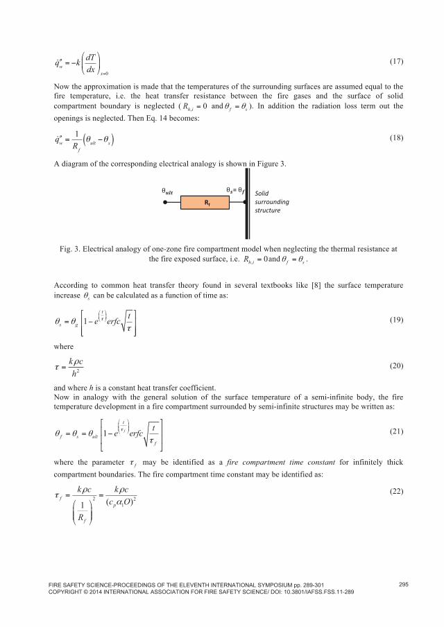
qw = k dTdx x=0

(17)

Now the approximation is made that the temperatures of the surrounding surfaces are assumed equal to the fire temperature, i.e. the heat transfer resistance between the fire gases and the surface of solid compartment boundary is neglected ( , 0h iR = and f s= ). In addition the radiation loss term out the openings is neglected. Then Eq. 14 becomes:

qw =1

Rfult s( ) (18)

A diagram of the corresponding electrical analogy is shown in Figure 3.

Fig. 3. Electrical analogy of one-zone fire compartment model when neglecting the thermal resistance at the fire exposed surface, i.e. , 0h iR = and f s= .

According to common heat transfer theory found in several textbooks like [8] the surface temperature increase s can be calculated as a function of time as:

1t

s gte erfc= (19)

where

2

k ch

= (20)

and where h is a constant heat transfer coefficient. Now in analogy with the general solution of the surface temperature of a semi-infinite body, the fire temperature development in a fire compartment surrounded by semi-infinite structures may be written as:

1 f

t

f s ultf

te erfc= = (21)

where the parameter f may be identified as a fire compartment time constant for infinitely thick compartment boundaries. The fire compartment time constant may be identified as:

2 21( )1

fp

f

k c k cc O

R

= = (22)


295

The relation to standard design time-temperature curves may be demonstrated by prescribing a maximum

temperature increase 2 1325ultpc= = (ºC) as derived above. Then if a fire compartment time constant

1200f = s is assumed, Eq.21 yields the fire temperature as an analytical solution as:

12001325 11200

t

fte erfc= (23)

Figure 4 shows the fire temperatures according to this analytical solution (Eq. 23). For comparison the standard fire curve according to ISO 834 and EN 1363-1 and the parametric temperature-time curve for a gamma value of unity according to Eurocode 1 (EN 1991-1-2) are also shown. Note that the three time-temperature curves are almost identical for the first three hours. The difference between the standard curve and the parametric curves is so small that it is not visible in this diagram. The analytically curve goes asymptotically to the ultimate temperature 1325 ºC while the ISO curve is defined by a log function and goes to infinity for long fire durations.

Fig. 4. Comparison between fire temperature rise according to the analytical expression (Eq.23) and the standard ISO 834/EN 1363 curve

In reality the heat transfer resistance between the fire gases and the surfaces of the compartment boundaries must be considered. If it is assumed constant it may be included in this type of simple linear analysis by adding the two resistances fR and hR , see Figure 2. The fire compartment time constant then becomes:

2

2 ( )1

f f h

f h

k c R R k c

R R

= = +

+

(24)

The surface temperature s may be obtained from Eq. 21 and the fire temperature f from Eq. 15. Below is an example to illustrate how fire temperatures of a compartment surrounded by infinitely thick structures with constant properties may be calculated as a function of time.

Example 1

Calculate the fully developed fire temperature increase after 60 min in a compartment surrounded by concrete.

a) Neglecting the effects of heat transfer resistance b) Considering the effects of heat transfer resistance


296

Assume an opening factor of 0.04 m½, a heat transfer coefficient of 70toth = W/(m2 K), and other fire compartment properties according to Table 2. For concrete assume the conductivity k=1.7, the density

=2300 kg/m3and the specific heat capacity c=900 J/(kg K)

Solution:

a) Eq. 11 yields 1 0.0435575 0.04fR = = (m2 K) /W

and Eq. 21 yields( )2

3530000 6673s575 0.04

f = = .

Thus 3600 0.546673f

t= =

Eq. 21 yields 0.541325 1 0.54 646f s e erfc C= = = °

b) Thermal resistance 1 1 0.014370h

tot

Rh

= = = (m2 K) /W

Eq. 24 yields 2

3530000 11793sec1

0.0435 0.0143

f = =

+

.

Thus 3600 0.30511793f

t= =

Eq. 21 yields 0.3051325 1 0.305 544s e erfc C= = °

and the fire temperature can be obtained from Eq. 15 as

544 0.0435 1325 0.0143 7370.0435 0.0143f C+

= = °+

(Thus the fire temperature is 90 C° higher when the heat transfer resistance is considered.)

Thin compartment boundaries

An analytical solution of the fire temperatures may also be obtained when the fire compartment is surrounded by structures consisting of a metal core where the all the heat capacity is concentrated. Thus the capacity per unit area coreC may be approximated as lumped into the core as indicated in Figure 5. In the analyses below the heat capacity of any insulating material are either neglected or considered as included in the heat capacity of the core. Figure 6 shows an electrical analogy of how the fire temperature and the core and the surface temperature can be calculated. Figure 6 indicates also the relative temperature increase initially, after some finite time and after a very long time. Since according to the model all inertia is lumped into the core and no inertia is assumed in the insulation layers, the temperature differences between various positions will always be proportional to the corresponding thermal resistances. In the analyses in this section the heat loss by radiation through the opening is neglected. Otherwise an analytical solution is not possible.


297

Fig. 5. A fire compartment surrounded by a structure with its heat capacity C assumed concentrated/lumped to a metal core. Thermal resistances iR and oR are assumed on the

fire inside and outside, respectively, due to insulation and heat transfer resistance.

Fig. 6. Electrical analogy of fire compartment model with a thin surrounding structure assuming lumped heat. Temperatures at various points initially (t=0), after some time (0 t ) and after a

very long time (t= ).

The thermal resistance on the inside (fire exposed side) iR of the core may be obtained as the sum of thermal heat transfer resistance and the conductive resistance as:

, ,i h i ins iR R R= + (25)

and correspondingly on the outside (unexposed fire side) as:

, ,o h o ins oR R R= + (26)

The total thermal resistance of the structure then becomes:

tot i oR R R= + (27)

The conduction resistance of the core is neglected. Then the maximum fire temperature rise may be derived from Eq. 8 as

max 2

1

1tot

f ultf tot

ptot

RR Rc

OR

= =++

(28)

and


298

max ocore ult

f tot

RR R

=+

(29)

where ult may be obtained from Eq. 10. fR is defined by Eq. 11. In iR and oR both the heat transfer resistance and possibly the conduction resistance are included. Fig. 7 shows the maximum fire temperature in a non-insulated steel container as a function of the opening factor assuming surface emissivities equal 0.8 and convection heat transfer coefficients according to Eurocode, i.e. 25 W/(m2 K) and 4 W/(m2 K) at the fire exposed and the non-fire exposed sides, respectively.

Fig. 7. Maximum fire and steel temperature of a non-insulated steel container as a function of the opening factor [9].

If all the parameters are constant the core temperature increase may be written as a function of time as

1 ft

totcore ult

f tot

R eR R

=+

(30)

As the insulation is assumed to have negligible heat capacity, the compartment fire temperature increase can be calculated as a weighted average between the ultimate fire and the core temperatures as

1 ft

oi fult

i f f core tot ff ult

f i f tot

RR R eR R R R

R R R R

++ +

= =+ +

(31)

In a corresponding way the fire exposed surface temperature becomes

, ,,

( )ultins i f f h i core

s if i

R R RR R+ +

=+

(32)

The fire compartment time constant f is

1 1core

f

f i o

C

R R R

=+

+

(33)

where coreC is the heat capacity per unit area of the core.


299

Example 2

A fire compartment is surrounded by a 3 mm thick steel sheet structure with a 12 mm thick gypsum board mounted on both sides of the core. The opening factor is 0.08 m½. The total heat transfer coefficient at the fire exposed and the unexposed sides are assumed to be 200 W/(m2 K) and 40 W/(m2 K), respectively. a) Calculate the ultimate fire temperature increase ult

b) Calculate the maximum fire maxf

and core maxcore temperature increases.

c) Calculate the core core and fire f temperature increases after 300 s of flash-over.

Solution:Use fire parameter values as given in Table 2. The conductivity of gypsum is assumed to be 0.5 W/(m K) and the specific heat capacity of steel equal 460 J/(kg K) and the density 7850 kg/m3.Thena) Eq. 10 (or Table 2) yields 1325ult = ºC. b) The thermal resistance on exposed side 0.0121 0.029200 0.5iR = + = (m2 K)/W

and the thermal resistance on unexposed side 0.0121 0.04940 0.5oR = + = (m2 K)/W.

The fire heat transfer resistance yields 1 0.0221150 0.5 0.08fR = = (m2 K)/W.

Then the maximum fire temperature increase (Eq. 28) will be

6max

3

1.52 10 103411.15 10

0.5 0.08 (0.029 0.049)

f = =+

+

ºC

and Eq.29 yields max 0.049 1325 6490.022 0.049 0.029core = =

+ + ºC.

c) Eq.33 yields 270f = s and temperature increase after 300 s can be obtained from Eq.30 as

3002700.0491325 1 1325 0.494 0.67 439

0.021 0.049 0.29core e= = =+ +

ºC

and from Eq.31 max 0.029 1325 0.021 439 9530.021 0.029f

+= =

+ ºC.

Numerical solutions of one-zone model fires

When the heat transfer model includes parameters varying with temperature including heat radiation through openings or layered compartment boundaries, a numerical procedure must be used. The finite element program Tasef [10] developed for calculating temperature in fire exposed structures allows for mixed boundary conditions and is therefore suitable for such purposes. For this type of calculations the heat transfer resistances have to be assumed constant or neglected.

qw =1

Rf + Ri

2

cps +

Ao

Atot

1

1+Rh,i

Rf

(T 4 Tf4 ) (14)

The surface temperature can now be calculated with, for example, the finite element code Tasef [10]with the analogue assumptions according to Table 1. A one-dimensional model of the surrounding structure is then assumed. This may then contain several layers of materials, materials with properties varying with


300

temperature, structures containing voids or anything that is possible to model with the code available. Work with these type of assumptions are under way at Luleå University of Technology, Sweden.

CONCLUSIONS

In this paper a new simple calculation method for analytically calculating compartment temperature when flashover is reached has been described. This new method introduces the so called ultimate fire temperature, the maximum temperature which can be reached when there is no energy lost in the compartment surroundings and no radiation lost through the openings. This temperature depends only on the combustion yield 2, combustion efficiency and the specific heat capacity of air cp, but it is independent of the air mass flow rate, and of the fire compartment geometry and the thermal properties of the compartment boundaries. A value in the order of 1325ult = ºC can then be deducted for a combustion efficiency of 50 % and the analytically derived time-temperature development is approximately the same as given in Eurocode 1 (EN 1991-1-2) as parametric temperature-time curves. In reality the heat is lost by radiation through the openings and the combustion efficiency is likely to be higher than 50 %. The first fact reduces the maximum temperature possible to reach while the latter would lead to increased temperatures.

In this paper the ultimate temperature for a compartment with semi-infinitely thick walls as well as with thin walls with a steel core and finite insulation has been used to calculate analytically compartment fire temperature. It has been shown that for semi-infinite case the solution match very well with the standard ISO 834/EN 1363-1 curve and with the parametric curves according to EN 1991-1-2. It has also been shown how the maximum fire temperature of a compartment with thin wall depends on the ultimate compartment fire temperature and the total thermal resistance of the surrounding structure.

ACKNOWLEDGEMENTS

The authors gratefully acknowledge the financial support provided by The Swedish fire research board, Brandforsk, Sweden.

REFERENCES

[1] Magnusson, S.E., Thelandersson, S., Temperature-Time Curves for the Complete Process of Fire Development - A Theoretical Study of Wood Fuels in Enclosed Spaces, Acta Politechnica Scandinavica, Ci 65, Stockholm, 1970.

[2] Wickström, U., Application of the Standard Fire Curve for Expressing Natural Fires for Design Puposes , Fire Safety: Science and Engineering, ASTM STP 882, T.Z. Harmathy, Ed., American Society of Testing and Materials, Philadelphia, 1985, pp.145-159.

[3] EN 1991-1-2, Eurocode 1: Actions on structures – Part 1-2: General actions – Actions on structures exposed to fire

[4] Babrauskas, V., Williamsson, R.B. Post-flashover compartment fires: basic of a theoretical model, Fire and materials, vol 2, No. 2, 1978, pp 39-53.

[5] Huggett,C., Estimation of rate of heat release by means of oxygen consumption measurements, Fire and Materials, volume 4, issue2, 1980, pp.61-65

[6] Tewarson, A.. Heat release in fires, Fire and Materials, 4, 1980, pp. 185-191.

[7] Drysdale D. An introduction to fire dynamics. Second edition. John Wiley & Sons publisher, 1998, p180.

[8] Holman, J.P. Heat transfer, McGraw-Hill Science/Engineering/Math, 10 edition, 2009.

[9] Sundström, O., Gustavsson, S., Simple temperature calculation models for compartment fires, Bachelor thesis, Luleå University of technology, 2012.

http://pure.ltu.se/portal/files/41431736/LTU-EX-2012-41368234.pdf

[10] Wickström, U., TASEF-2 – A Computer Program for Temperature Analysis of Structures Exposed to Fire”, Lund Institure of Technology, Department of Structural Mechanics, Report NO. 79-2 (doctoral thesis), Lund, 1979.


301

Paper B3

Temperature of post flashover compartment

fire –calculations and validation

by Alexandra Byström, Ulf Wickström

Journal of Fire and Materials, 2017

*Corresponding authour:Alexandra Byström, Division of Structural and Fire Engineering, Luleå University of Technology, Luleå 971 87. Sweden. Email: [email protected]

TEMPERATURE OF POST-FLASHOVER COMPARTMENT FIRES – CALCULATIONS AND

VALIDATION

Alexandra Byström*a & Ulf Wickströma

a Luleå University of Technology, Department of Civil, Environmental and Natural Resources Engineering, Luleå, Sweden

ABSTRACT

This paper describes and validates by comparisons with tests a one-zone model for computing temperature of fully developed compartment fires. Like other similar models, see overview [1], the model is based on an analysis of the energy and mass balance assumingcombustion being limited by the availability of oxygen, i.e. a ventilation controlledcompartment fire. However, the mathematical solution techniques in this model have been altered. To this end, a maximum fire temperature has been defined depending on combustion efficiency and opening heights only. This temperature together with well-defined fire compartment parameters was then used as a fictitious thermal boundary condition of the surrounding structure. The temperature of that structure could then be calculated with various numerical and analytical methods as a matter of choice and the fire temperature could be identified as a weighted average between the maximum fire temperature and the calculated surface temperature of the surrounding structure as a function of time.

It is demonstrated that the model can be used to predict fire temperatures in compartmentswith boundaries of semi-infinitely thick structures as well as with boundaries of insulated and non-insulated steel sheets where the entire heat capacity of the surrounding structure is assumed to be concentrated to the steel core. With these assumptions, fire temperatures could be calculated with spread-sheet calculation methods. For more advanced problems, a general finite element solid temperature calculation code (TASEF) was used to calculate the temperature in the boundary structure. With this code it is possible to analyze surrounding structures of various kinds, for example structures comprising several materials with properties varying with temperature as well as voids.

The validation experiments were accurately defined and surveyed. In all the tests a propane diffusion burner was used as the only fire source. Temperatures were measured with thermocouples and plate thermometers at several positions [2].

KEYWORDSPost-flashover compartment fire, fire temperature, validation, fire modelling.

INTRODUCTION

Several researchers have studied compartment fires experimentally and several models havebeen published on estimating post-flashover compartment fire development, see e.g. [1,3]. In

1963, Kawago and Sekine [4] proposed one of the first time-temperature curves by assumingventilation controlled fires with constant heat release rates. In the 1970s, Magnusson and Thelandersson [5] calculated fire time-temperature curves based on heat and mass balance analyses. Their model is known as the Swedish opening factor method. It was later modified by Wickström [6] and became the Eurocode parametric fire curves, EN 1991-1-2, Annex A. Babrauskas developed a computer program for calculating post-flashover fire temperatures, COMPF2, [7] and used it to derive closed-form algebraic equations to estimate temperaturedevelopment in post flashover compartment fires [8]. Moreover, a comprehensive review of existing correlation models can be found in the SFPE Engineering Guide to Fire Exposures to Structural Elements [1] .

There are several computer models for calculating fire temperature [9]. In zone models such as CFAST [10] or BRANZFIRE [11], the enclosure is divided into two zones: the hot upper smoke layer and lower layer. Temperatures inside each layer are assumed to be uniform. Zone fire models are capable of predicting the environment in a multi-compartment structure subjected to a fire. For instance, CFAST calculates the time evolution distribution of smoke and fire gases and the temperature throughout a building during a user-prescribed fire [10].According to the user guide for CFAST [10], the thermo-physical properties of the boundaries are held at constant value. In addition, only one single layer of material per boundary is allowed (some earlier versions allowed up to three). It means that the effect ofmoisture content in the material cannot be taken into consideration, the same goes for temperature dependent material properties and voids.

The model presented here is based on the early work by Magnusson and Thelandersson [5].They developed graphical fire curves depending on ventilation and thermal properties of surrounding structures. Both their model and this new model are based on the energy balance of a single fire compartment. However, with a new way of analyzing the energy equations the fire temperature as a function of time may in some idealized cases be calculated by analytical closed form expressions [12]. An ultimate and a maximum fire temperature can also be defined depending on the combustion efficiency and opening heights only, while the rate of fire temperature increase depends on the thermal properties of the boundaries and on the relation between the mass flow rate and the total surrounding area of the compartment. The mass flow rate is assumed to be constant and proportional to the opening area times the square root of its height for fully developed fires when a uniform fire temperature is assumed.

The new approach presented in this paper may use finite element modelling for calculating fire temperature. It gives the opportunity to accurately consider boundary structures with several layers including materials with temperature dependent properties as well as voidswith radiation and convection heat exchange. Thus non-linear effects due to latent heat caused by water evaporation may for example be considered. Previous models are not able to accurately consider such effects. By making certain approximations, simple spread-sheet calculations may be used for calculating the fire temperatures and in some cases even closed form analytical solutions may be derived [12,13].

In this paper, fire temperatures of a series of experiments are compared with calculated temperatures. In all experiments referenced here a propane gas burner was used with a constant heat release rate of 1000 kW. The results of the entire test series is summarized and can be downloaded from the internet [6].

BACKGROUND

Heat balance of flashed over compartment fires

The heat balance of a fully developed fire compartment as indicated in Figure 1 may be written:

c l w rq q q q [1]

where cq is the heat release rate in the compartment by combustion of fuel, lq the heat loss rate due to the flow of hot gases out of the compartment openings, wq the losses to the compartment boundaries and rq the heat radiation out through the openings. Other components of the heat balance equation are in general insignificant and are not included in a simple analysis as this.

Figure 1. Heat balance for the post-flashover compartment fire.

One-zone fire model for flashed over fires

Due to conservation of mass, the gas flow rate out of the compartment om must be equal to the mass flow rate of the fresh air entering the compartment im (the mass of the gases generated by the fuel is neglected):

i o am m m [2]

For vertical openings, the flow rate is assumed to be proportional to the opening area times the square root of its height:

1a o om A h [3]

where 1 is a proportionality factor and, oA and oh are the area and height of the openings of the compartment, respectively. According to [15], when the gas temperature inside the compartment exceeds 800 K, the mass flow rate into the compartment will be proportional to the area and height of the opening. The proportionality constant 1 is called a flow constant.

Here it is assumed 512

kg0.5s m

.

The combustion rate cq inside a ventilation controlled compartment is proportional to the mass flow rate and can be written as:

wqwq

wq

wq

cqlq

rqom

im

Uniform temperature

fT T

2c aq m [4]

where is the combustion efficiency and 2 a constant describing the combustion energy developed per unit mass of air [12]. The combustion yield constant is assumed to be

62

Ws3.0 10 kg and is obtained from the knowledge that most organic materials yield

about 13.1·106 Ws per kg oxygen under ideal combustion conditions and this varies very little for different fuels [16]. The yield constant 2 is calculated assuming that the mass fraction of oxygen is 23 % in the ambient air.

The combustion efficiency is usually assumed to be in the range of 40 % - 70 % according to Drysdale [17]. A value of 60 % is assumed in the analyses of this paper. This gives goodcorrelations with experimental data. However, the efficiency is an uncertain parameter in any model. As a general rule it will decrease when fires become fuel rich or ventilation controlled, which have been reported by for example Tewarson in 1980 [18]. Unburnt fuel may then burn outside the fire compartment.

The convection loss term is proportional to the mass flow times the fire temperatureincrease, i.e:

( )l p a f iq c m T T [5]

where pc is the specific heat capacity of the combustion gases. Here pc is assumedtemperature independent having the same value as of air with temperature 800 ºC. According to Holman [19] the value of the specific capacity of air varies with temperature in the narrow range of 1.00·103 Ws/(kg K) at 20 ºC to 1.2·103 Ws/(kg K) at 1000 ºC. fT and iT are the fire and ambient temperatures, respectively.

The heat loss to the compartment surfaces wq is proportional to the total surrounding area of the enclosure, totA :

w tot wq A q [6]

where wq is the heat flux rate to the enclosure surfaces. This term constitutes the inertia of the system [12].

Finally the heat radiating out through the openings may be calculated as:

4 4( )r o fq A T T [7]

where T is the ambient temperature, which is assumed to be equal to the initial temperature,

iT T .

Ultimate fire temperature, ultT [12]

Consider a closed compartment without radiation losses through the openings and perfectlyinsulated boundaries, i.e. no heat loss through the boundaries. Then by inserting Eq. [4]andEq. [5] into the heat balance equation (Eq. [1]) and assuming 0wq and 0rq we get:

2 ( ) 0 0a p a f im c m T T [8]

In this case a very high temperature can be reached, the so called ultimate compartment fire temperature rise [12,13], ult , obtained from Eq.[8]:

2ult f i

p

T Tc

[9]

The ultimate compartment fire temperature, ult ult iT T , will not be obtained in reality as fire compartments have openings where heat will be lost by radiation. Exceptions may be furnaces and tunnels which have no openings directly to areas at ambient temperatures. Then very high temperatures might therefore develop. The ultimate compartment fire temperatureis introduced here to facilitate the derivation and explanation of the fire temperature development model.

Maximum fire temperature, maxT

Let us now assume that the compartment has perfectly insulated boundaries, i.e. no heat loss through the boundary ( 0wq ), but heat is lost by radiation out through the opening(s). Byinserting Eq.[4], Eq.[5] and Eq.[7] into the heat balance equation Eq.[1], we get:

4 42 ( ) 0 ( )a p a f i o fm c m T T A T T [10]

Solving Eq.[10] with respect to fT will give the maximum compartment fire temperature

maxT which can be reached when the losses to the walls vanishes.

Some simplification can here be made. Inserting Eq.[3] into Eq.[10] and dividing both sides by 1( )p o oc A h gives:

2 22

1

( )( )1 f f

fp p o

T T T Tc c h

[11]

where f is the fire temperature increase defined as:

f f iT T [12]

By inserting Eq.[9] and rearranging Eq.[12] with respect to f we get:

max 2 2

1

ˆ ˆ( )( )1

ult

f f

p o

T T T Tc h

[13]

Note that this equation, Eq.[13], is implicitly stated, since maxˆ

f iT T .

Also notice that the maximum fire temperature, fT in Eq[13]., depends on the square root of

the opening height, oH , but is independent of oA and totA .

Fire temperature in flashed over compartments, fT

By inserting Eq.[4]-[7] into Eq.[1] we get:4 4

2 ( ) ( )a p a f i tot w o fm c m T T A q A T T [14]

If we then replace am according to Eq.[3] and rearrange, we get

4 421 ( )o

w p f fp tot

Aq c O T Tc A

[15]

where O is the so called opening factor defined as

o o

tot

A hO

A[16]

Eq.[15] is analogous to the heat transfer equation by convection and radiation between a gas and a solid surface [13]. This may be seen as an analogous electrical model as shown in the left part of Figure 2. Eq. [15] can then be written as:

. .

1 1 ( )w ult f ff c f r

q T TR R

[17]

where the fire compartment artificial thermal resistance due to convective heat transfer is

.. 1

1 1f c

f c p

Rh c O

[18]

and the fire compartment artificial thermal resistance due to radiation heat transfer is

. 2 2.

1 1ˆf r

f r f f

Rh T T T T

[19]

in which the ratio o

tot

AA can be associated by analogy with an emissivity, i.e. ˆ o

tot

AA .

Figure 2. Electric circuit analogy of the fire compartment boundary according Eq. [17] and Eq. [21].

The total heat transfer to any surrounding surface by convection and radiation is

w con radq q q [20]

Thus the heat transfer at the exposed fire surface can be seen as an analogous electrical modeland Figure 2 (right side) can be written as:

. . .

1 1 1( )w f s f s f si c i r i tot

q T T T T T TR R R

[21]

where the total thermal resistance is identified as:

.

. .

11 1i tot

i r i c

RR R

[22]

and the thermal resistance due to convective heat transfer between fire temperature and surface temperature is:

..

1i c

i c

Rh

[23]

The convective heat transfer coefficient, .i ch , for the walls in the enclosure can be assumed to be in the order of 25 W/m2K on fire exposed sides as recommended in Eurocode (EN 1991-1-2).Moreover, the fire compartment thermal resistance due to radiation heat transfer is:

. 2 2.

1 1i r

i r s f s f s

Rh T T T T

[24]

where s is emissivity of the exposed surfaces which depending on material is in the order of 0.8.

The two temperatures ultT and T in Figure 2 may for calculation reasons be reduced to one resultant temperature maxT , which is a weighted mean value of the two, similar to the theory behind the adiabatic surface temperature [13]. Then the electric circuit of Figure 2 can be simplified as shown in Figure 3.

.f cR.i cR

ultT

fT sT

wq


.i rR.f rRT

According to Figure 3 and the heat transfer theory described above, the fire temperature fTcan be obtained as a weighted mean temperature of maxT , Eq.[13], and sT , as

. max .

. .

s f tot i totf f i

f tot i tot

T R T RT T

R R[25]

Figure 3. Electric circuit analogy of the fire compartment boundary, and a diagram indicating maximum, fire and surface temperatures, repectively, initially (t=0), after

[12,13].

Fire temperature in flashed over compartments – assumption for FE modeling with Tasef, fT

For the numerical analysis reported here the combustion efficiency is assumed to be 60 % as mentioned above. This will give a ultimate compartment fire temperature, Eq.[9], of

20 1592ult ultT [°C] and a maximum temperature according to the theory above, Eq.[13].

Eq.[15] can be interpreted as a boundary condition for a fictitious surface with a temperature fT exposed to radiation and convection where the heat transfer is expressed as:

4 4.( ) ( )w f f c ult fq T T h T T [26]

T.f totR .i totR

maxTfT sT

maxT ( )fT t ( )sT t

(0 )sT t

(0 )fT t

( 0)fT t

( 0)sT t

ultT

T

wq


The heat flux to the compartment surrounding structure by convection and radiation depending on fT is then calculated according to Eq[21]. As there is no inertia the temperature fT can be calculated as a weighted average as indicated in Figure 3.

The above theory will be used for the numerical analysis with parameters defined in Table 1.All parameters which have been used in the model are collected in Table 2. Both ambient and initial temperatures are assumed to be 20 °C.

Table 1. Analogue artificial heat transfer parameters for FE-modelling with Tasef.

Emissivity Convection heat transfer coefficient

Ultimate fire temperature

ˆ o

tot

AA . 1f c ph c O 2

ult ip

T Tc

Table 2. Values of physical parameters.

Parameter Notation, value, units

Flow constant2.51 0.5kg

m s

Combustion yield coefficient 62 3.01 10 Ws

kg

Specific heat capacity of the combustion gases 1150pWsc kg K

EXPERIMENTAL SETUP

The experiments were conducted at the SP Fire Research. For more data and information about the experimental setup and result, see the report [2].

The enclosure was intended to represent a 3/4-scale version of an office room. The inner dimensions of tests series A, C and D were 1800 mm by 2700 mm and 1800 mm high.Centrally on one of the short ends was a 600 mm by 1500 mm high doorway opening, see Figure 4. The materials and thicknesses of the walls were changed between the test series.The same materials were used in floor, ceiling and walls for each set of experiments.

Figure 4. Inner dimensions of the enclosure.

A diffusion propane burner (300 mm by 300 mm) was placed in the middle of the enclosure.The gas burner was filled to half its volume with gravel (~10-20 mm stones). The heat release rate was kept constant at rate of 1000 kW in the tests analyzed in this paper.

Light weight concrete (LWC) boundaries. The first experiment (Test A1) was conducted in a compartment with the structures containing its original moisture. The density of the material was measured before testing to be around 760 kg/m3, containing 39 % of moisture (mass of water/mass of dry material). The second experiment (Test A5) was conducted in the same compartment after a series of four experiments. Then it can be assumed that the concrete had dried out. More details for the original concrete as well as after exposure in a furnace heated to 105 °C during 24 h are found in Table 3.

Insulated steel boundaries. Test series B (Test B2) was conducted in a 3 mm thick steel structure. The inner dimensions of the steel enclosure were as shown in Figure 4. However, the width/length/height of the inner surfaces in test series B were 100 mm smaller as the inside was covered with 50 mm stone wool boards, i.e. the inner dimensions were then 1700by 2600 by 1700 mm. Test series D (Test D2) was conducted on the same steel structure as test series B but with the stone wool insulation on the outside. So the inner dimension was the same as presented in Figure 4. The stone wool had a nominal density of 200 kg/m3 and a nominal room temperature conductivity of 0.04 W/mK.

Non-insulated steel boundaries. Test series C (Test C2) was conducted in the same steel structure as test series B but without any insulation.

1800 mm

1500

mm

600 mm

Table 3. Nominal thermal material properties at room temperature [2].

Material Specific heat, (J/kgK)

Thermal conductivity at room temperature, (W/mK)

Density, (kg/m3)

Light weight concrete, original(before heating)

851 0.330 760

Light weight concrete, dried (exposed to 105°C for 24 h)

835 0.166 -

Stone wool 800 0.04 200

Several thermocouple trees were installed to measure gas temperatures at various heights [2].A total of more than 50 insulated Plate Thermometers (insPT) [20] and thermocouples were mounted inside the compartment and in the door opening. In this paper only the insPT temperatures were selected for analyses and comparisons with calculated temperatures.

NUMERICAL ANALYSIS

To calculate surface temperatures according to the theory described above, the finite element code Tasef [21] was used.

A one-dimensional heat transfer FE analysis was carried out as indicated by Figure 5. For the Tasef analysis, the total heat transfer resistance between the fire gases and the exposed surface, .i totR (Eq.[22]) was modelled as an artificial element with a thermal resistance according to the relation:

.. . .

ˆ1 1ˆi tot

i c i r i tot

lRh h h k

[27]

The value of conductivity for the artificial element with size of ˆ 1l mm is indicated in Figure 6. The specific heat capacity and density were kept at a very low value to not disturb the accuracy of the thermal model. The convective heat transfer coefficient, .i ch , for the walls in the enclosure was assumed equal to 25 W/m2K on exposed to fire sides and the radiative heat transfer coefficient, .i rh , was calculated according to Eq.[28]

3. 4i r sh T [28]

The heat transfer coefficient by convection on the unexposed side, conh , was assumed equal to 4 W/m2K. The emissivities of the surfaces, s , were assumed equal to 0.8 on both the exposed and the unexposed sides, see Figure 5.

Figure 5. Electric circuit analogy model of heat transfer analysis with Tasef according to the new model, and finite element model inluding an artifical boundary element modelling the heat transfer

conditions at the fire exposed side.

Figure 6. Total heat transfer coefficient translated to thermal conductivity of the artificial element with thickness of 1 mm, according to Eq.[27].

The measured light-weight concrete properties of the enclosure boundaries, as mentioned above, were applied in the FE-analysis. The material properties of steel were assumed according to Eurocode 4 and producer available data for stone wool, respectively [22]. The data was extrapolated for higher temperatures, as shown in Figure 7. For the concrete, the

,f cRultT

fT .i sT

wq


,f rRT ,i totR

ˆ

.f ch

T

ultT

Convective heat

Radiation heat

Convective heat

Radiation heatArtif

icia

lele

men

t (k

(T)~

hi,to

t(T))

k, , c

T s

T conh

,o cR

,o rR

.o sT T


structure

(k, , c)

0

0.2

0.4

0.6

0.8

1

1.2

0

200

400

600

800

1000

1200

0 300 600 900 1200 1500

Cond

uctiv

ity o

f art

ifici

al e

lem

ent,

[[W

/mK]

Tota

l hea

t tra

nsfe

r coe

ffici

ent,

[W/m

2K]

Temperature, [°C]

effects of water evaporation were considered by the input of the specific volumetric enthalpy [21] to TASEF.

Figure 7. Thermal conductivity of the stone wool used for the FE-modeling.

The specific volumetric enthalpy (material input parameter in TASEF) or the heat content of the material at a specific temperature T above zero [13] is expressed by Eq.[29]:

0( )

T

ii

e T cdT l [29]

where and c are density and specific heat capacity, respectively. The last term ii

l refers

to latent heats due to for example of evaporation moisture [13].

NUMERICAL ANALYSIS USING FDS

Additional simulations were performed using the Fire Dynamics Simulator (FDS) version 6.0 [23] to analyse the conducted experiments. The FDS software solves the Navier-Stokes equations in the limit of low-speed, thermally-driven flow with an emphasis on smoke and heat transport from fires.

In this work, the simulations were done in accordance with the experimental setup [2] using the same heat release rates, geometrical set-up and location of devices and extracting similar outputs as in the experimental scenarios described earlier in [2]. The material data is taken from measurements, as described above. In the model, a propane diffusion burner is introduced that supplies the same constant heat release rates as in the experiment. Plate thermometers are introduced as physical objects to be able to account for the time delay due to inertia of the plate thermometer. This model has been described in [24].A 5 cm mesh resolution was chosen [25]. The heat release was kept constant as in the experiment.

RESULTS AND DISCUSSIONS

Plate thermometers (PT) measure approximately the adiabatic surface temperature (AST), an effective temperature which can used as a third kind or Robin boundary condition [13] when calculating heat transfer by radiation and convection to structures exposed to fire, see e.g.[26–28]. These temperatures are therefore deemed to be the most relevant for representing the

0

0.1

0.2

0.3

0.4

0.5

0.6

0 200 400 600 800 1000 1200

The

rmal

con

duct

ivity

[W/m

K]

Temperature [°C]

Taken from KIMMCOStonewool

Assumed/Extrapolate

fire compartment temperatures. Maximum and minimum temperatures measured with PT are given in Appendix.

Approximately the same final/maximum temperatures were measured in all the insulated cases (A5 – LWC, B2 – insulation inside and D2 – steel insulation outside), see Figure 11and Figure 12. The maximum temperature which can be computed from the theory above,Eq.[13], (1207 ºC) agreed very well with the maximum measured temperature during the experiments. The temperature increase rate, i.e. the time history to reach the final temperature is, however, very different in the three cases. The compared to mineral wool high density ofthe LWC requires a long time to reach the final temperature, whereas in the B-series, the insulation inside the enclosure reaches final temperatures after only a few minutes. When the insulation is on the outside of the steel, the inertia of the fire exposed steel significantly delays the time to reach equilibrium. With non-insulated steel, the final temperature is several hundred degrees lower than the final temperatures of all the other cases as a considerable amount of heat is then lost through the surrounding structure even when equilibrium is reached.

The numerically calculated fire temperature histories have been compared with measured temperatures. Two fire experiments conducted in the light weight concrete compartment,moist (as originally) (Test A1) and dry (Test A5), respectively, are shown in Figure 8. The agreement between measured and calculated temperatures is deemed satisfactory for bothcases. Note – in Figure 8 that the effect of moisture evaporation on the temperature development is considered very accurately by the numerical analysis. The moisture content makes the temperature development rate remarkably slower.

Figure 8. Measured and calculated fire temperatures in the LWC compartment (Tmax calculated with Eq.[13]) . Left: Originally moist concrete, test A1. Right: Dry concrete, test A5.

The same type of calculation was done for the steel sheet compartment without insulation (Test C2) and with insulation on the inside (Test B2) and on the outside (Test D2), respectively. The measured maximum temperature was compared with the temperature calculated with Eq.[13], see Figure 9. For the non-insulated steel sheet compartment, the calculated fire temperatures were compared with the measured mean temperature, see Figure 10. The material properties of the insulation were assumed temperature dependent as shown in Figure 7. Good agreements between measured and calculated temperatures were obtained

0

200

400

600

800

1000

1200

1400

0 10 20 30 40 50

Tem

pera

ture

, [ºC

]

Time, [min]

Test A1, measured Test A1, calculated

Tmax

0

200

400

600

800

1000

1200

1400

0 10 20 30 40 50

Tem

pera

ture

, [ºC

]

Time, [min]

Test A5, measured Test A5, calculated

EN 1991-1-2 Tmax

as shown in the diagrams of Figure 9 and Figure 10. Observe that the fire temperature of the steel compartment with insulation on the inside rises much faster to the maximum temperature than when the insulation is on the outside. The calculated fire temperature in the non-insulated steel compartment depends very much on the assumed heat transfer conditions on both the exposed and unexposed surfaces as these constitutes the only thermal resistances between the inside and outside of the fire compartment. The maximum temperature measured, 800 ºC, is significantly lower than the maximum temperatures measured in all the insulated compartments.

Figure 9. Measured and calculated fire temperatures in the steel sheet compartment (Tmax calculated with Eq.[13]). B2-insulated inside, C2-non-insulated and D2-insulated outside.

Figure 10. Measured and calculated fire temperatures in the non-insulated steel compartment.

The fire temperature reaches about 1200 °C (Eq.[13]) max 1207T °C) during test A, test B and Test D, see Figure 8 and Figure 9, while for the non-insulated case the final measured temperature reaches only around 800 °C, see Figure 10.

0

200

400

600

800

1000

1200

1400

0 10 20 30 40 50

Tem

pera

ture

, [ºC

]

Time, [min]

Test B2, measured Test B2, calculated

EN 1991-1-2 Tmax

0

200

400

600

800

1000

1200

1400

0 10 20 30 40 50

Tem

pera

ture

, [ºC

]

Time, [min]

Test D2, measured Test D2, calculated

EN 1991-1-2 Tmax

0

200

400

600

800

1000

1200

1400

0 10 20 30 40 50

Tem

pera

ture

, [ºC

]

Time, [min]

Test C2, measured_ T_MAX

Test C2, calculated

Test C2, measured_T_Mean

Note that this calculation model yields good predictions particularly in terms of the qualitative development of the fire temperature, i.e. the influences of the thermal properties of the various compartment boundaries on the maximum temperatures and temperature rise rates are well predicted.

A corresponding parametric fire temperature curve according to EN 1991-1-2 was also plotted. As can be seen in Figure 8 and Figure 9, it overestimates in these cases the fire temperature increase for the concrete structure beyond 10 minutes. For the insulated steel structure the fire temperature reaches its maximum within seconds both according to this new model and to the Eurocode parametric curve.

Temperatures calculated with FDS agreed impressively well with measured temperatures for all cases, see Figure 11 and Figure 12 in Appendix. However, in comparison with the model presented here, it requires extensive input data such as prescribed HHR, detailed geometry, etc. and the computing time is extensive. As an example, a simulation of test series A1 with amesh size of 5 cm and a duration of 60 minutes takes around 24 hours on a modern PC. On the other hand, a much more detailed temperature output is obtained as well as other parameters like species concentrations and smoke densities.

CONCLUSIONS

With this new compartment fire model formulation, the maximum temperatures of post-flashover fires as well as the temperature rise rate can be predicted depending on a variety oftypes of boundary structures. One-dimensional FE analyses of this type of problems are very fast and results are computed within a second on modern PCs. This novel mathematical formulation has made it possible to use FE temperature analyses for accurately predicting compartment fire temperatures. Use of FE software gives the possibility for considering combinations of materials and non-linearities like material properties varying with temperature and latent heat due to moisture evaporation.

Two important temperatures for the general understanding of compartment fires were identified:

1. Ultimate temperature, Eq.[9] – the highest temperature that can be reached in acompartment where heat loss by radiation and heat loss by conduction into the boundary can be neglected.

2. Maximum temperature, Eq.[13] - the highest temperature that can be reached in acompartment where the heat loss by conduction into the boundary can be neglected.

A new formulation of a one-zone fire model has been validated with experiments conducted in compartments of light weight concrete and steel sheets, insulated on the outside and on the inside as well as non-insulated. The overall conclusions from the validation tests were:

1. Maximum temperature reached after a long time (Eq. [13]) is in good agreement with measurements.

2. Fire temperature vs time calculated with this new model is in good agreement with the highest temperatures measured in the compartment.

3. Effects of moisture in the boundary structure (Test A1 and Test A5) are predicted very well.

4. Parametric fire temperature curves according to EN 1991-1-2 over-estimate the temperature for the LWC structure and the insulated steel sheet structures (not relevant for the non-insulated case).

5. FDS predicted the fire temperatures impressively well for all the cases, see Appendix.

The main uncertainty parameter in this model is combustion efficiency of the fuel. The value of 60 % is used here for all cases.

APPENDIX. COMPARTMENT FIRE TEMPERATURESExperimentally measured and calculated with FDS

The mean temperature from the experiments and FDS simulations is calculated from theaverage temperature to the fourth power (the radiative potential) from all readouts of the PT measurements around the whole compartment, see Eq.[30].

4. .

4.

PT i PT iPT mean

tot

T AT

A[30]

In test series A, there were 26 PTs in total and for the rest of experiments, 19. To compensate for “missing data” for the tests series B, C and D, some assumptions were made, see Table 4.For more detailed information of the location of PT, see report [2].

Table 4. Location of the PTs.

Position of PT Test series A Test series B, C and DRight wall Five PTs, see[2]Left wall Five PTs, see[2].

Symmetric positions to right wall

Two PTs on the upper positionAdditional three PTs in the center and lower

positions – right wallCeiling Five PTs, see[2]Floor Four PTs, see [2] Two PTs on the right position

Additional two PTs – assumed symmetric Front wall Four PTs, see [2] Two PTs on the right position

Additional two PTs – assumed symmetricBack wall Three PTs, see [2]

Figure 11. Experimental results vs FDS simulation of the light weight concrete tests: A1 and A5,showing compartment maximum, mean and minimum measured and calculated PT temperatures.

0200400600800

10001200

0 10 20 30 40 50

Tem

pera

ture

, [°C

]

Time, [min]

Concrete, Test A1Max. Temp., measured Max. Temp., FDS

Mean Temp., measured Mean Temp., FDS

Min. Temp., measured Min. Temp., FDS

0200400600800

10001200

0 10 20 30 40 50

Tem

pera

ture

, [°C

]

Time, [min]

Concrete, Test A5Max. Temp., measured Max. Temp., FDS

Mean Temp., measured Mean. Temp., FDS


Figure 12. Experimental results vs FDS simulation of the steel compartment tests, insulated on the inside -B2 and outside -D2, non-insulated – C2, showing compartment maximum, mean and minimum

measured and calculated PT temperatures.

ACKNOWLEDGMENTS

The authors are grateful to Johan Sjöström at SP Research for managing and conducting the fire tests. The Swedish fire research board, Brandforsk is gratefully acknowledged for providing financial support for this work.

REFERENCES[1] SFPE, SFPE Engineering Guide to Fire Exposures to Structural Elements, Society of

Fire Protection Engineers, Bethesda, MD, 2004.

0200400600800

10001200

0 10 20 30 40 50

Tem

pera

ture

, [°C

]

Time, [min]

Steel insulated on the inside, Test B2

Max. Temp., measured Max. Temp., FDS



0200400600800

10001200

0 10 20 30 40 50

Tem

pera

ture

, [°C

]

Time, [min]

Steel insulated outside,Test D2




0200400600800

10001200

0 10 20 30 40 50

Tem

pera

ture

, [°C

]

Time, [min]

Uninsulated steel, Test C2




[2] J. Sjöström, U. Wickström, A. Byström, Validation data for room fire mo

background, Borås, Sweden, 2016.[3] W.D. Walton, P.H. Thomas, Estimating Temperature in Compartment Fires, in: SFPE

Handbook of Fire Protection Engineering, Third Edit, National Fire Protection Association, Quincy, Massachusetts, 2002.

[4] K. Kawagoe, T. Sekine, Estimation of Fire Temperature-Time Curve in Rooms, Tokyo, Japan, 1963.

[5] S.E. Magnusson, Thelandersson, Temperature-Time curves of complete process of fire development, Stockholm, 1970.

[6] U. Wickström, Application of the standard fire curve for expressing natural fires for design purposes, Fire Safety: Science and Engineering. 882 (1985) 145–157. doi:10.1520/stp35295s.

[7] V. Babrauskas, COMPF-2 - A program for calculating post-flashover fire temperatures. Technical note 991, Washington, DC, 1979.

[8] V. Babrauskas, A closed-form approximation for post-flashover compartment fire temperatures, Fire Safety Journal. 4 (1981) 63–73. doi:10.1016/0379-7112(81)90005-9.

[9] S.M. Olenick, D.J. Carpenter, An Updated International Survey of Computer Models for Fire and Smoke, Journal of Fire Protection Engineering. 13 (2003) 10–12. doi:10.1177/104239103033367.

[10] R.D. Peacock, P. a. Reneke, G. Forney, CFAST - consolidated model of fire growth and smoke trasport (Version 7). Volume 2: User’s guide, National Institute of Standards and Technology, 2015.

[11] C.A. Wade, A User’s Guide to BRANZFIRE 2004, 2004.[12] U. Wickström, A. Byström, Compartment fire temperature - a new simple calculation

method, in: Fire Safety Science - Proceedings of the Eleventh International Symposium, 2014: pp. 289–301. doi:10.3801/IAFSS.FSS.11-289.

[13] U. Wickström, Temperature calculation in fire safety engineering. 1st Edition, Springer International Publishing, 2016. doi:10.1007/978-3-319-30172-3.

[14] Validation data for room fire models, (2016). https://www.researchgate.net/publication/303862845_Validation_data_for_room_fire_models.

[15] V. Babrauskas, R.B. Williamson, Post-flashover compartment fires: Basis of a theoretical model, Fire and Materials. 2 (1978) 39–53. doi:10.1002/fam.810020202.

[16] C. Huggett, Estimation of rate of heat release by means of oxygen consumption measurements, Fire and Materials. 4 (1980) 61–65. doi:10.1002/fam.810040202.

[17] D. Drysdale, An introduction to fire dynamics. Second Edition, John Wiley & Sons, Ltd, England, 1998.

[18] A. Tewarson, Heat release rate in fires, Fire and Materials. 4 (1980) 185–191. doi:10.1002/fam.810040405.

[19] J.P. Holman, Heat Transfer. Tenth Edition., 10th Editi, McGram-Hill Science/Engineering/Math, 2009.

[20] J. Sjöström, U. Wickström, Different Types of Plate Thermometers for Measuring Incident Radiant Heat Flux, in: 13 Th International Conference and Exhibition on Fire Science and Engineering, Interflam, Royal Holloway College, Nr Windsor, UK, 2013: pp. 363–371.

[21] U. Wickström, TASEF-2 – A Computer Program for Temperature Analysis of Structures Exposed to Fire, Lund Institute of Technology, 1979.

[22] KIMMCO Facade insulation (KFI), (2014).

http://www.kimmco.com/kimmco/english/glasswool-kfi.asp.[23] K. McGrattan, S. Hostikka, R. Mcdermott, J. Floyd, C. Weinschenk, K. Overholt,

NIST Special Publication 1019. 6th Edition. Fire Dynamics Simulator User’s Guide, 2015. doi:10.6028/NIST.SP.1019.

[24] R. Jansson, J. Anderson, Experimental and numericla investigation of fire dynamics in facade test RIG., in: International Congress on Fire Computer Modeling, Santander, Spain, 2012.

[25] A. Byström, J. Sjöström, J. Anderson, U. Wickström, Validation of a one-zone room fire model with well-defined experiments, Luleå, Sweden, 2016.

[26] U. Wickström, A. Robbins, G. Baker, The Use of Adiabatic Surface Temperature to Design Structures For Fire Exposure, Journal of Structural Fire Engineering. 2 (2011) 21–28. doi:10.1260/2040-2317.2.1.21.

[27] A. Byström, X. Cheng, U. Wickström, M. Veljkovic, Measurement and calculation of adiabatic surface temperature in a full-scale compartment fire experiment, Journal ofFire Sciences. 31 (2012) 35–50. doi:10.1177/0734904112453012.

[28] A. Byström, J. Sjöström, U. Wickström, D. Lange, M. Veljkovic, Large Scale Test on a Steel Column Exposed to Localized Fire, Journal of Structural Fire Engineering. 5 (2014) 147–160. doi:10.1260/2040-2317.5.2.147.

Paper B4

Pre flashover compartment fires – calculations

and validations

by Alexandra Byström, Ulf Wickström

Pre-flashover compartment fire temperature: a new calculation model validated with experiments

ALEXANDRA BYSTRÖM and ULF WICKSTRÖM Division of Structural and Fire Engineering/ Department of Civil, Environmental and Natural Resources Engineering Luleå University of Technology, 971 87, Luleå, Sweden [email protected]@ltu.seABSTRACT A new two-zone model for computing temperature of pre-flashover compartment fires is introduced. It is validated by comparisons with very accurately defined and controlled experiments. This model predicts upper layer fire temperatures in compartments with semi-infinitely thick boundaries as well as with boundaries of insulated or non-insulated steel sheets. The mass flows of air and fire gases are assumed controlled by the plume entrainment depending on a prescribed heat release rate and plume height. The combustion is limited by the rate at which gaseous fuel (pyrolysis gases) is released. The model is based on the assumption that the heat release rate is equal to the heat lost by convection of air and radiation out through the opening(s) and by losses to the surrounding structures.

For a constant heat release rate, this model yields the maximum upper layer temperature a fire would reach when lasting for a very long time as well as the fire temperature as a function of time depending on the inertia, on the design of the surrounding structure and on the ventilation conditions of the compartment.

KEYWORDS: two-zone fire model, flashover, compartment fire temperature, model validation.

NOMENCLATURE LISTING A area [m2]

oA area of openings [m2] C capacity per unit area [J/( m2.K)] c specific heat capacity [J/(kg.K)]

pc specific heat capacity at constant pressure [J/(kg.K)] d core thickness [m] H height of enclosure [m]

oh height of openings [m] h heat transfer coefficient [W/(m2.K)] k conductivity [W/(m.K)] L length of enclosure [m] l thickness of material [m]

mass flow rate of gases [kg/s] R heat resistance [m2.K/W] T temperature [K or ºC]

iT initial temperature [K or ºC] t time [s]

heat flux [W/m2] cq heat release rate by combustion [W]

W width of enclosure [m] oW width of openings [m]

z effective height of the plume [m]

Greek symbols 1 flow constant [kg/(s.m2.5)]

2 constant describing the combustion energy developed per unit mass of air [W.s/kg]

3 correlation factor [kg/(s.W1/3.m5/3)] combustion efficiency [-]

emissivity [-] temperature difference [K] density [kg/m3]

time constant [s] Stefan–Boltzmann constant [W/(m2.K4)]

Superscripts * pre-flashover model . per unit time " per unit area

Subscripts

ambient a air AST Adiabatic Surface Temperature c convection core core of structure f fire F.O flashover i inside/in ins insulation k conduction L air replacement LWC light weight concrete max maximum o outside/out p plume PT plate thermometer r radiation s surface t total tot total ult ultimate w wall

1. INTRODUCTIONDuring the ignition and growth phases of a fire, temperatures in the compartment are generally moderate and are not a threat to structures. The fire intensity is then limited by the amount of available pyrolysed gaseous fuel and can be defined as a fuel-controlled or pre-flashover fire.

So called two-zone numerical models, e.g. CFAST [2] or BRANZFIRE [3] and more sophisticated computerized fluid dynamics, CFD, codes such as the Fire Dynamics Simulator, FDS, [4] may be used for analyzing pre-flashover fires. In two-zone models, the temperature of the hot gas layer or zone depends on the amount of heat being released and on the thermal properties of the surrounding structure.

Evegren and Wickström [5] presented a new numerical model for estimating temperatures in pre-flashover container fires where the heat capacity of the fire enclosure boundaries are assumed to be lumped in the surrounding steel. Their model is applicable for structures of non-insulated and insulated steel sheets. This pre-flashover model is derived using the same

approach as for the ventilation controlled fire model presented in [6,7] but is based on the assumption of a prescribed heat release fuel controlled fire [5] and that the mass flow depends on fire plume entrainment of air. Evegren and Wickström described their model by an electric circuit analogy with the steel core as a capacitor and the heat resistances of the boundaries and the insulation as electrical resistances. Their model was implemented in an MS-Excel application.

Models for predicting temperature of hot gases in fuel-controlled or pre-flashover compartment fires are generally empirical. For example, the frequently used model of McCaffrey, Quintiere and Harkleroad, known as the MQH model [8], was derived based on comparisons with tests and on the assumptions that the heat losses to surrounding structures depend on the structures’ thermal properties.

The model for pre-flashover as presented here is based on the theory described by Wickström [6]. It resembles the model developed for post-flashover fires [6,7].

2. TWO-ZONE FIRE MODEL FOR PRE-FLASHOVER FIRES

2.1 Conservation of mass

In pre-flashover models, the heat release rate cq is an input parameter. All combustion is assumed to occur inside the fire compartment boundaries and is limited by the rate at which gaseous fuel (pyrolysis gases) is being released from burning objects. As shown in figure (Fig. 1), an upper layer uniform temperature fT is then supposed to develop. Below, the lower layer gas temperature remains at the ambient temperature T . In this paper it is assumed that the ambient, T , and initial, iT , temperatures are equal, i.e. iT T

Hot gases generated by the combustion enter the upper layer via the fire plume, i.e. ambient air is continually entrained over the plume height. The flow rate pm at which mass is entering the upper layer is assumed equal to the mass flows in im and out om of the compartment, i.e.

p i om m m (1)

The plume mass flow rate is calculated as a function of the heat release rate cq and of the height between the fuel surface and the upper smoke layer interface. This is in contrast to post-flashover fires where the heat release rate inside the compartment is assumed to depend only on the flow rate of the air into the compartment which in turn depends on the size and height of the opening(s).

wq

wq

wq

, pmcq om

im

fT

T

wqlq

rq

Fig. 1. Two-zone model of a pre-flashover room fire with uniform temperature fT in the upper

layer and ambient gas temperature T in the lower layer.

The mass flow rate can be obtained by an iteration procedure from correlation models of the ideal plume flow rate by Zukoski et al, Thomas or Heskestad [9]. The plume flow rate pm by Zukoski [10] was used for this analysis, thus:

513 3

3p cm q z (2)

where z is the effective height of the plume above the burning area and is usually assumed to be the height of the smoke layer interface above the floor. The constant

3 5 13 3

0.0071 kg

m W s was experimentally determined by Zukoski, [10].

The flow rate for vertical openings in a fully developed compartment fire is the maximum flow rate that can be reached, i.e. . .p a F Om m , where pm comes from Eq.(2) and

. . 1a F O o om A h , [7]. This gives us an expression for the maximum effective height of the plume above the burning area:

31 5

31 3 c o oz q A h (3)

2.2 Heat balance The energy balance for a fire compartment can be written:

c l w rq q q q (4)

where cq is the heat release rate in the compartment by combustion of fuel, lq the heat loss rate due to the flow of hot gases out of the compartment openings, wq the losses to the compartment boundaries and rq the heat radiation out through the openings. This is similar to the situation for the post-flashover compartment fire models described by e.g Wickström [6]. The last term is less significant for pre-flashover fires due to lower fire temperatures and is therefore very often not taken into consideration [8,9]. Other components of the heat balance equation are in general insignificant and are not included in a simple analysis as this.

The combustion rate cq inside a fuel controlled compartment is an input parameter. It must not exceed the maximum combustion rate for a ventilation controlled compartment fire [7,9],

which is proportional to the mass flow rate for a fully developed fire [7,11] and can be written as:

1 2c o oq A H (5)

where is the combustion efficiency and 2 a constant describing the combustion energy developed per unit mass of air [7]. The combustion efficiency is usually assumed to be in the range of 40% - 70% according to Drysdale [12]. Tewarson [13] suggested, however, that combustion efficiency values can be up to 99% for methanol.

Flashover is generally defined as the transition from a growing fire, a so called pre-flashover fire, to a fully developed fire, a post-flashover fire [14]. In this study, flashover is supposed to occur when the combustible fuel gases balance the amount of oxygen available for combustion. Then the Heat Release Rate needed for flashover is:

. . 2 . . . 1 2F O a F O o oq m A H (6)

Observe that according to this definition, the occurrence of flashover depends only on the opening but is independent on the size and thermal properties of the surrounding structure.

The convection loss term is proportional to the mass flow rate out through the opening, om , times the fire temperature increase, i.e:

( )l p o fq c m T T (7)

where pc is the specific heat capacity of the combustion gases (usually assumed equal to that of air), here 1150pc (W·s)/(kg·K) and fT and T are the fire and ambient temperatures, respectively.

By using Eq.(1) and inserting Eq.(2) into Eq.(7), we get: 51

3 33 ( )l p c fq c q z T T (8)

The heat lost to the compartment surfaces wq is proportional to the total surrounding area of the exposed enclosure (without openings), totA :

w tot wq A q (9)

where wq is the heat flux rate to the enclosure surfaces. This term constitutes the inertia of the system [7]. Energy/heat is stored in the surrounding structure as it gradually heats up, therefore the heat losses to the surrounding structures decrease as the surrounding surfaces heats up.

As shown in Fig. 1, the upper layer is then supposed to develop a uniform fire temperature fT . In the lower layer, the gas temperature remains at the ambient temperature T . The heat is assumed lost to all compartment boundaries uniformly. This is justified by the fact that the heat transfer to the surrounding surfaces is dominated by radiation which is independent of gravity.

Finally the heat radiating out through the openings can be calculated as: 4 4( )r o f fq A T T (10)

where the emissivity f is here a reduction coefficient considering that not the entire opening is radiating in contrary to the one-zone fire model.

2.3 Fire temperature By going back to the definition of heat balance and by inserting Eq.(8), Eq.(9) and Eq.(10) into Eq.(4), we get:

51 4 43 33 ( ) ( )c p c f i tot w o f fq c q z T T A q A T T (11)

The heat balance equation of a compartment fire can be rearranged to be analogous to the heat transfer equation by convection and radiation between a gas and a solid surface [6,7].

Then Eq.(11) gives the general formulation of the new model for pre-flashover compartment fire:

51 23 3 33 4 4

53

3

( )p c o fcw f f

tot totp

c q z Aqq T TA Ac z

(12)

By assuming natural/mixed boundary conditions [6], the heat transfer wq to any surface can be expressed in terms of the radiation, gas and surface temperatures:

'' 4 4( ) ( )w c g s s r sq h T T T T (13)

where in this equation ch , gT , s and rT are boundary input constants and sT is an unknown surface temperature. Eq.(12) is analogous to this equation as described in the details below.

2.4 New calculation model

Ultimate fire temperature

Assume a compartment without radiation losses through the openings and with perfectly insulated boundaries, i.e. no heat loss through the boundaries. By inserting Eq.(8), 0wq and

0rq in the heat balance equation, Eq.(4) , we get:

513 3

3 ( ) 0 0c p c f iq c q z T T (14)

In this case, the ultimate pre-flashover compartment fire temperature rise *ult is reached. By

assuming a constant prescribed heat release rate, Eq.(14) yields: 2

3*

53

3

cult f i

p

qT Tc z

(15)

The ultimate compartment fire temperature, * *ult ult iT T , will in reality not be obtained since

fire compartments have openings where heat will be lost by radiation. The ultimate pre-flashover compartment fire temperature is introduced here to facilitate the derivation and explanation of the fire temperature development model. Notice that the ultimate temperature used in this model is not the same as the ultimate temperature defined for the post-flashover compartment fire model [7], which is the highest temperature that can be reached in that

compartment, 2. .ult F O

pc .

Maximum fire temperature

Let us now assume that the compartment has perfectly insulated boundaries, i.e. no heat losses through the boundary. By inserting Eq.(8), Eq.(10) and 0wq in the heat balance equation, Eq.(4), we get:

51 4 43 33 ( ) 0 ( )c p c f i o f fq c q z T T A T T (16)

Solving Eq.(16) with respect to fT gives the maximum compartment fire temperature *maxT

that can be reached when the losses to the walls are neglected.

Analogous electrical model

Eq.(12) is analogous to the heat transfer equation by convection and radiation between a gas and a solid surface. This may be seen as an analogous electrical model, see Fig. 2. Eq.(12) can here be rewritten as:

*

. .

1 1w ult f f

f c f r

qR R

(17)

where iT T and f f iT T are the ambient and fire temperature rise, respectively. The fire compartment thermal resistance due to convective heat transfer can be identified from Eq.(12) and Eq.(16) as:

. 513 3. 3

1 totf c

f c p c

ARh c q z

(18)

and the fire compartment thermal resistance due to radiation heat transfer is:

. 2 2.

1 1ˆf r

f r f f

Rh T T T T

(19)

in which the ratio o f

tot

AA can be defined as an analogous emissivity, i.e. ˆ o f

tot

AA .

The two temperatures *ultT and T can be reduced to a single resultant temperature *

maxT . Here *

maxT is the maximum temperature a compartment fire can reach in a pre-flashover compartment fire for a given cq , when the losses to the walls vanish. It can be defined as a

weighted mean value of *ultT and T , see Eq.(16). This can be done in a similar way as in the

theory behind the adiabatic surface temperature [6]. The electric circuit representing the heat transfer that can be seen in Fig. 2 can now be reduced to the one in Fig. 3.

* *. .*

max *. .

f c f r ult

f c f r

R T R TT

R R (20)

where by analogy with the theory behind the adiabatic surface temperature, the fire compartment thermal resistance due to radiation heat transfer is

*. * 22 * *. max max

1 1

ˆf r

f r

Rh T T T T

(21)

.f cR .i cR*

ultT

fT sT

wq

.i rR.f rRT

Fig. 2. Electric circuit analogy model of a fire compartment boundary according to the new model.

Heat transfer at the surface

The total heat transfer to any surrounding surface by convection and radiation is: w con radq q q , which according to [6] and Fig. 2, can be written as:

. . .

1 1 1( )w f s f s f si c i r i tot

q T T T T T TR R R

(22)

where the total thermal resistance is identified as

.

. .

11 1i tot

i r i c

RR R

(23)

where the thermal resistance due to convective heat transfer between the fire and the surrounding surfaces is:

..

1i c

i c

Rh

(24)

The convective heat transfer coefficient, .i ch , for the walls in the enclosure can be assumed to be around 25 W/m2K on exposed to fire sides and around 4 W/m2K on unexposed sides (EN 1991-1-2).

Moreover, the fire compartment thermal resistance due to radiation heat transfer is:

. 2 2.

1 1i r

i r s f s f s

Rh T T T T

(25)

where s is the emissivity of the exposed surfaces.

By inserting Eq.(25) and Eq.(24) into Eq.(23) we get that the thermal resistance between the fire temperature fT and the surface sT , is:

. 2 2

.

11i tot

s f s f si c

RT T T T R

(26)

As there is no thermal heat capacity involved, the heat flux may also be written, see Fig. 3, as: **

maxmaxmax max

. . . .

f f ssw

f tot i tot f tot i tot

T T T TT TqR R R R

(27)

where the total artificial fire compartment thermal resistance from *maxT and fT is

max.

max..

11 1f tot

f cf r

RRR

(28)

in which .f cR , Eq.(17), is the artificial fire compartment thermal resistance due to convection

and max.f rR is the artificial fire compartment thermal resistance due radiation heat transfer from

maxT to fT :

max. 2* 2 *

max max

1

ˆf r

f f

RT T T T

(29)

max.f totR .i totR

*maxT fT sT

.f cR.i cR

fT sT

wq


.i rRmax.f rR

*maxT


wq

Fig. 3. Modified electric circuit analogy model of a fire compartment boundary, based on the definition of the maximum fire temperature.

3 UPPER LAYER FIRE TEMPERATURE In combination with the boundary conditions defined by Eq.(27), Eq.(20) and Eq.(4), the temperature of a surrounding structure may be calculated in a similar way as for one-zone models [6,7], where the boundary condition on sides exposed to fire is defined as two heat transfer resistances in series, as indicated in Fig. 3: one artificial between *

maxT and fT and one physical between fT and sT .

According to the lower electrical chart of Fig. 3, the boundary condition may be expressed by two thermal boundary resistances in a series. These can be combined into one by adding them together and thus it becomes a third kind of boundary condition [6] by definition. A third kind of boundary condition (sometimes called a natural or Robin boundary condition) means that the heat flux to the boundary depends on the difference between a specified surrounding gas temperature and a surface temperature. In its simplest form, the heat flux is proportional to the difference between the surrounding gas temperature and the surface temperature. The proportionality constant is denoted the heat transfer coefficient h and thus the heat flux at the boundary can be expressed as:

0w g x

x

Tq h T T kx

(30)

In the case of compartment fires, we generally need numerical methods that can be modelled in MS-Excel or finite element methods in order to compute the surface temperature. The fire temperature is then calculated as a weighted mean temperature of *

maxT and sT (see Fig. 3) as: max *

. max .max

. .

s f tot i totf

f tot i tot

T R T RT

R R (31)

where max.f totR , Eq.(28), is the artificial thermal resistance between *

maxT and the fire temperature

fT , and .i totR is the real thermal resistance between the fire temperature fT and the surface

sT , Eq.(26).

The surface temperatures may be calculated by analytical and numerical means depending on whether the model parameters may vary with temperature. When either heat transfer coefficients/resistances or material properties are assumed to vary with temperature, the problem becomes non-linear and numerical tools such as finite element programs need to be used. Boundary structures of several layers of different materials etc. may then also be considered.

Analytical closed form expressions can be derived for two types of boundary constructions: structures assumed either semi-infinitely thick or having a core where the thermal mass is concentrated (lumped heat), and both the real .i totR and artificial boundary conditions max

.f totR are assumed constant.

4.1 Semi-infinite thick compartment boundary Compartment boundaries can in most cases be assumed thermally thick for the short durations of most fires.

Analytical solution Given all parameters being assumed constant, an analytical closed form solution of the surface temperature may be derived. This solution is based on the above general formulation of a pre-flashover compartment fire model Eq.(12) and on the analogy with the solution of the surface temperature of a semi-infinite body that can be found in text-books like [15]. Then the surface temperature of a semi-infinite structure may be written as:

*max 1 f

t

sf

te erfc (32)

where * *max max iT T must be assumed constant, maxT is defined by Eq.(20) or Eq.(16) and

depends on that cq must be constant for the analytical solution to be valid. Here the surface temperature rise is s s iT T , t is time and f may be identified as a fire compartment time constant for infinitely thick compartment boundaries that can be calculated as

2max.. .2max.co

. .

const constf f tot i totnst const

f tot i tot

k c k c R RR R

(33)

By Eq(32), the surface temperature can be obtained at any time, t , with the assumptions of constant heat release rate, constant material properties ( , ,k c ) and constant thermal heat transfer coefficients/resistances, as

max.. 3

max* max. ..

1 11 1 1ˆ4

constf tot

f c f cf r

RTR RR

(34)

. 3.

. ..

1 1 1ˆ1 1 1(4 )

consti tot const

i tot const s fi c i ci r

Rh TR RR

(35)

where ..

1i c

i cR h is the thermal resistance by convection heat transfer on unexposed sides of

the enclosure and ˆfT is a representative value of the fire temperature fT and the surface

temperature sT . Hence the total thermal resistance according to Eq.(35) depends on the

representative temperature ˆfT and can be obtained from the diagram of Fig. 4. With an

increase of the temperature, the resistance between the fire temperature fT and the surface temperature sT becomes insignificant. Moreover, the upper layer fire temperature can be calculated as a weighted average between sT and *

maxT according to Eq.(31).

0

0.01

0.02

0.03

0.04

0 200 400 600 800 1000

Tota

lhea

ttra

nsfe

rres

ista

nse,

[m2.

K/W

]

Representative temperature [ºC]

Ritot

Fig. 4. Relation between temperature and resistance .

consti totR , according to Eq.(35).

Numerical solution The surface temperature of semi-infinitely thick compartment boundaries with boundary conditions according to Eq.(27) may also be solved numerically with e.g. finite element methods. Then the material and heat transfer conditions may vary with temperature.

4.2 Insulated and non-insulated steel compartment boundaries A system which may be considered uniform in temperature can be analysed by the lumped heat capacity method. In general, the smaller the physical size of a body and the higher the conductivity (like metals), the more realistic the assumption of uniform temperature throughout [15].

Analytical solution Analytical solutions of fire temperatures may be obtained when the fire compartment is assumed surrounded by structures consisting of a metal core where all the heat capacity is assumed concentrated, i.e. the heat capacity per unit area coreC is lumped into the core, see Fig. 5. In addition, the heat capacity of any insulating material is either neglected or assumed included in the heat capacity of the core.

T

.f cR

*maxT

T

*ultT

T

wq

( )coreT t

(0 )coreT t

.i insRmax

.f rR

.o cR

.o rR

.i cR

.i rR.o insR*

maxT T

.s oT.s iT coreTfT

*ultT

T

T

( 0)coreT t Fig. 5. Electric circuit analogy model of a fire compartment boundary surrounded by

structures consisting of a metal core, according to the new model. As the temperature of the core is uniform, the heat transfer to the core is:

corecore core

dTq c ddt

(36)

and since the heat balance of the core yields, core i oq q q , the increase in the core temperature over a time step t may be written as

1i icore core i o

core

tT T q qc d

(37)

where based on the electrical circuit analogy model of the heat flux to the core (see Fig. 5), iq and oq can be defined as:

*max

max.. . .

icore

i const constf tot i tot i ins

T TqR R R

(38)

. .

icore

o consto ins o tot

qR R

(39)

in which max..

constf totR is the artificial thermal resistance between *

maxT and the fire temperature

fT . In a similar way as for semi-infinite surroundings, the thermal heat transfer resistances

can be assumed constant according to Eq.(34). Here .consti totR is the thermal resistance between

the fire temperature fT and the surface temperature .s iT and can also be kept constant according to the theory described above for semi-infinite surroundings, Eq.(35) and Fig. 4.

insins

ins

lR k is the thermal resistance of the insulation material and .consto totR is the thermal

resistance between the unexposed surface .s oT and the fire ambient temperature T :

. 2 2. . .

. ..

1 1 11 1 1

consto tot const

o tot const s s o s oo c o co r

Rh T T T TR RR

(40)

where the thermal resistance by convection heat transfer ..

1o c

o cR h , in which the convective

heat transfer coefficient, .o ch , for the walls on unexposed sides of the enclosure can be assumed to be around 4 W/m2K (EN 1991-1-2).

By using the general solution of Eq.(36) for the lumped-heat capacity of the metal core, see [6,15] and Fig. 5, and by inserting Eq.(38) and Eq.(39), the core temperature rise can be calculated analytically at time t as:

* . .max max. *

. . . . .

1 expconst

o ins o totcore const const const

f tot i tot i ins o ins o tot f

R R tR R R R R

(41)

As the insulation is assumed to have negligible heat capacity, the compartment fire temperature increase can be calculated as a weighted average between the maximum fire temperature and the core temperature, see Fig. 5, as:

*max . . . .

max. * max.. . . . . . . .

max..

1 exp1

const consto ins o tot i tot i ins

f const const const const consti tot i ins f tot i tot i ins o ins o tot f f tot

constf tot

R R R RtR R R R R R R R

R (42)

where the temperature rise iT T , *maxT is defined from Eq.(20) or Eq.(16) and the time

constant *f is calculated as

*

max.. . . . .

1 1core

f

const const constf tot i tot i ins o ins o tot

C

R R R R R

(43)

where core coreC c d is the heat capacity per area of the core.

The surface temperatures .s iT , Eq.(44), and .s oT , Eq.(45), may then be calculated from:

max. max.

. . .

cores i const const

f tot i tot i ins

T TTR R R

(44)

.. .

cores o const

o tot i ins

T TTR R

(45)

Numerical solution More accurate solutions for the core temperature and the fire compartment temperature can be obtained by the step-by-step numerical procedure according to Eq.(46) and Eq.(47), whereby the material and in particular the heat transfer conditions can be updated at each time step Thus the core and fire temperature rise can be calculated numerically by the forward difference method:

1 max*.

. . . . .

i ii i core corecore core i i i i i

core f tot i tot i ins o ins o tot

tC R R R R R

(46)

11 1 max

. .*.. . .

ii i i icoref core i tot i insi i i

f tot i tot i ins

R RR R R

(47)

where the thermal resistances are updated at each time increment depending on the temperature. By analogy with the analytical solution, the surface temperature on exposed and unexposed sides of the structure may be calculated from:

11 max

. max.. . .

ii core

s i i if tot i tot i ins

T TTR R R

(48)

11

.. .

ii core

s o io tot i ins

T TTR R

(49)

4 EXPERIMENTAL SETUP A set of experiments in reduced scale was conducted at the SP Fire Research [1]. In most of them, the effect needed for flashover to occur was reached. However, two experiments did not reach flashover and were therefore chosen for the analyses here. One took place in a compartment with 100 mm light weight concrete boundaries and one in a compartment with 3 mm non-insulated steel sheets.

The inner dimensions of the tested compartments were 1800 mm by 2700 mm and a height of 1800 mm representing an office room in scale 3:4. Centrally on one of the short ends was a 600 mm by 1500 mm high doorway opening, see Fig. 6. The same materials were used for the floor, ceiling and walls for each set of experiments. For more data and information about the experimental setup and result, see the report [1].

A propane diffusion burner (300 mm by 300 mm) was placed in the middle of the enclosure. The gas burner was filled to half its volume with gravel (~10-20 mm stones). The heat release rate (HRR) was kept constant at 500 kW, which did not cause any flashover.

1800 1500

1800600

Fig. 6. Left: inner dimensions of the enclosure. Right: test object of lightweight concrete,

from [1]. For the calculations, the density of the dried concrete material used was assumed to be 547 kg/m3, the specific heat capacity 835 J/(kg·K) and the thermal conductivity 0.166 W/(m·K). The density and heat capacity of the steel were assumed to be 7850 kg/m3 and 460 J/(kg K), respectively.

Several thermocouple trees were installed to measure gas temperatures at various heights [1]. Insulated Plate Thermometers (insPT) [16] together with thermocouples were mounted both inside the compartment and in the door opening. In total, more than 50 measuring devices were installed. In this paper, only the readout from the insulated Plate Thermometers (insPT) measurements were selected and compared with calculated temperatures.

5 SOLUTION OF COMPARTMENT FIRE TEMPERATURE WITH NEW MODEL For estimating the compartment fire temperature, some assumptions were introduced:

1. The emissivities of the surfaces, s , were assumed equal to 0.8 on both the exposed and unexposed sides.

2. The convective heat transfer coefficient .i ch for the walls in the enclosure was assumed equal to 25 W/m2K on sides exposed to fire.

3. The heat transfer coefficient, .o ch , for the walls outside the enclosure was assumed to be around 4 W/(m2K) as recommended in EN 1991-1-2.

4. The emissivity of the fire f was assumed to be 0.5.

5. The effective plume height z was assumed to be depending on the opening height and in this analysis equal to / 2oH , i.e. 0.75z m

6. The ultimate temperature for the pre-flashover fire, according to Eq.(15), is 22 3 33

*5 5

3 33

500 1020 1266

0.0071 1150 0.75c

ult i

p

qT Tc z

ºC

7. The maximum temperature for the pre-flashover fire, according to Eq.(20) or Eq. (16), max 1064T ºC

5.1 Analytical and simplified numerical solutions

Light weight concrete (LWC) semi-infinite boundaries

To compute the fire temperature as a function of time t analytically when the surrounding structures are assumed semi infinitely thick, the thermal heat transfer coefficient/resistance must be kept constant according to Eq.(34). The constant fire resistance value that can be calculated according to Eq.(34) is max.

.1

25.8const

f totR (m2K)/W. In the case of a semi-infinite

structure, a high value of the representative fire temperature ˆfT can be assumed. For this study

the value of ˆ 800fT °C (see Fig. 4) was used, which gives the constant thermal resistance

between the fire and the exposed surface according to Eq. (35), .1

250consti totR (m2K)/W.

Hence the fire compartment time constant for infinitely thick compartment boundaries

according to Eq.(33) becomes: 21 10.166 547 835 13925.78 250f s. The fire

temperature and the surface temperature at any time t can then be calculated by Eq.(31) and Eq.(32), accordingly.

Uninsulated steel boundaries A similar procedure for analytical calculation was done for non-insulated steel boundaries. On the exposed side, a lower value of the representative fire temperature ˆ

fT can be assumed. For

this study, a value of ˆ 470ofT C (see Fig. 4) was used, which gives the constant value of the

thermal resistance between the fire and exposed surface according to Eq.(35), .1100

consti totR

(m2K)/W. The thermal heat transfer resistance on the unexposed side of the structure in the case of a non-insulated steel structure is assumed to be .

125

consto totR (m2K)/W, according to

Eq.(40) for a representative constant surface temperature on the unexposed side of . 370o

s oT C .

In this case, the fire compartment time constant according Eq.(43) becomes: 1

1 1460 7850 0.003 2201 1 10 025.78 100 25f s. The fire temperature and the

surface temperature at any time t can then be calculated by Eq.(42) and Eq.(41), accordingly.

5.2 Spread sheet modelling In addition, the steel core and fire temperatures were calculated numerically according to Eq.(46) and Eq.(47), respectively with MATLAB. The fire temperature at step (i+1) was obtained using the thermal resistances for step (i).

5.3 FE-modelling The purpose of using finite element modeling is to consider boundary and material properties varying with temperature. More complex surrounding structures can accurately be considered including effects of voids [11] and of moisture [17].

To calculate surface temperatures according to the theory described above, the finite element code TASEF [18] was used. Due to the experimental setup (the same material of the walls, ceiling and floor), a one dimensional FE analysis was used, see Fig. 6. Material properties for the LWC and steel were assumed constant and not temperature dependent. For the FE analysis, the boundary conditions according to Eq. (17) can be described as boundary conditions by heat exchange due to convection and radiation as:

* 4 4. ˆw f c ult f fq h (50)

where the input values for the FE analysis according to Eq.(50) are presented in Table 1. The values presented in Table 1 are calculated based on a constant HRR of 500 kW and on the assumptions of an effective height 0.75z m and a fire emissivity of 0.5f .

For the numerical analysis with TASEF, the total heat transfer resistance between the fire gases and the exposed surface, .i totR , Eq.(26), was introduced as an artificial element with

thermal conductivity material properties according to the relation ..

ˆ1ˆi tot

i tot

lRh k

. The

specific heat capacity and density were kept at the lowest possible values allowing the code to run smoothly. The radiative heat transfer coefficient .i rh was calculated according to Eq.(25).

Table 1. Parameters for the FE-analysis, according to Fig. 7.

Emissivity, ˆ o f

tot

AA

Convective heat transfer coefficient,

Eq.(18)51

3 33

.p c

f ctot

c q zh

A [W/mK],

Ultimate temperature Eq.(15), *

ultT [ºC]

0.018 16 1266

,f cR*

ultT

fT .i sT

wq


,f rRT ,i totR

ˆ

.f ch

T

*ultT

Convective heat

Radiation heat

Convective heat

Radiation heatArtificial

elem

ent

(k(T

)~hi

,tot(T

))

k, , c

T s

T conh

,o cR

,o rR

.o sT T


structure

(k, , c)

Fig. 7. Electric circuit analogy of the heat transfer TASEF analysis.

6 RESULTS AND DISCUSSIONS Both experiments analyzed and discussed in this paper were pre-flashover compartment fires with a constant HRR of 500 kW, which does not cause flashover according to Eq.(6) .

Calculated temperatures according to the new model were compared with Plate Thermometer (PT) measurements as they were deemed to yield the most representative temperatures. Thus, measured maximum and mean temperatures were compared with the numerically calculated fire temperatures. The mean temperatures were calculated based on the average temperature to the fourth power (the radiative potential) from all readouts of the PT measurements around the whole compartment. For details on the measurements, see [19].

PTs measure approximately the adiabatic surface temperature (AST), which is an effective temperature when calculating heat transfer by radiation and convection to structures exposed to fire, see e.g. [20–22]. The differences between temperatures measured with PTs compared to the AST are due to response time and heat conduction loss. The difference can be compensated for by the expression [21] :

PTPT

AST PT PT PTr c

dTCdtT T

h h (51)

where PTC [J/m2K] is the heat capacity coefficient of the PT, PTch and PT

rh are the convective and radiation heat transfer coefficients, respectively, where

2 2PTr AST PT AST PTh T T T T (52)

The plate thermometer is sensitive to convection and radiation in a similar way as a real specimen, due to a large sensor surface, in this case 100 mm by 100 mm. Therefore the value of PT

ch is assumed equal to the convective heat transfer coefficient for the walls in the enclosure, i.e. 25PT

ch W/(m2K). However, the value of PTrh is small in comparison to PT

ch , see Eq.(52). The difference in the initial stage of the experiment (the first 3 minutes) between the calculated AST and the corresponding mean value of the PT measurements during the non-insulated steel container experiment is shown in Fig. 8.

0

100

200

300

400

500

600

700

0 10 20 30

Tem

pera

ture

,[ºC

]

Time, [min]

T_AST

T_PT

Fig. 8. AST from PT measurement corrected according to Eq.(51) in the non-insulated steel

compartment. LWC compartment: Approximately the same final temperatures were measured as those calculated with the new model assuming semi-infinite surrounding structures analytically according to Eq.(31) as well as those calculated numerically with TASEF, see Fig. 9 a). For the calculations presented in this paper, values of 0.5f and 0.75z m were assumed. For these assumptions the calculated maximum temperature, see Fig. 9 a), max 1064T ºC, agreed well with the maximum measured temperature of about 1000 ºC after one hour.

However, the effective height of the plume, z , and the emissivity of the fire/opening, f , are uncertain parameters in this model. To estimate the effect of these parameters on the compartment fire temperature, the fire temperature was also calculated with the maximum effective height according to Eq.(3), 0.9z m, and with the assumption that heat radiates out through the opening based on a uniform fire temperature, 1f . The temperatures thus obtained are shown in Fig. 9 b), denoted ‘Calculated_analytical_modified’. They can be seen as lower bounds of the analytical solutions and correlate very well with the mean measured temperature by PTs, see Fig. 9 (right). This is a very crude sensitivity analysis, but it indicates the relative influences of various parameters as well as the robustness of the calculation model of the fire compartment temperature.

0

200

400

600

800

1000

1200

0 10 20 30 40 50 60

Tem

pera

ture

,[ºC

]

Time, [min]

Tmax_Eq.(16)

Measured_max_temp

Calculated_TASEF

Calculted_analytical_Eq.(31)

0

200

400

600

800

1000

1200

0 10 20 30 40 50 60

Tem

pera

ture

,[ºC

]

Time, [min]

Tmax_Eq.(16)_modified

Measured_mean_temp.

Calculated_analytical_modified

a) b)

Fig. 9. Calculated and measured fire temperatures in the LWC compartment. Non-insulated steel container: In the compartment with non-insulated steel boundaries, the final temperatures reached after 30 minutes were about 800 °C [1], which is several hundred degrees lower than the final temperatures reached in the LWC compartment.

Calculated temperatures with the new model compared with the AST according to Eq.(51) based on the mean PT measurements are shown in Fig. 8. As shown in Fig. 10, there is good agreement between the AST and calculated temperatures, both analytically, Eq.(42), and numerically, Eq.(47), as well as with TASEF.

0

100

200

300

400

500

600

700

0 10 20 30

Tem

pera

ture

,[ºC

]

Time, [min]

T_AST

Calculated_TASEF

Calculated_analytical_Eq.(42)

Calculated_numerical_Eq.(47)

Fig. 10. Fire temperatures in the non-insulated steel compartment.

7 CONCLUSIONS This paper demonstrates a new model for estimating temperature development in pre-flashed over fires. The model is based on heat and mass balance analyses of fire compartments in a similar way as for post-flashover fires as presented in [6,7]. The main differences are that the mass flow rate is governed by the plume entrainment, rather than the opening size and height, and that the heat release rate is an input parameter. This model was validated with experiments with a constant heat release rates from a gas diffusion burner conducted in compartments of light weight concrete and non-insulated steel, respectively. The fire temperature as a function of time calculated with this new model was in good agreement with corresponding measured temperatures.

Alternative numerical solutions with MS-EXCEL or MATLAB and with the finite element code, TASEF, gave almost identical results. By using FE methods, combinations of materials

and non-linearities due to material properties varying with temperature and moisture content (latent heat) can be considered. The only input data needed for this new simple model is geometry of the enclosure including openings and material properties of enclosure boundaries and a prescribed HRR.

This new model yields good predictions particularly in terms of the qualitative development of the fire temperature as function of time, i.e. the final maximum temperature as well as the temperature rise rate. Although the model is simple and the calculations are fast, it still clearly takes into account the basic physics of heat transfer and thermodynamics and is therefore an interesting alternative and complement to traditional two-zone modelling and CFD calculations.

8 FUTURE RESEARCH The model needs to be further validated with more experiments. Thus, influences of uncertain parameters such as fire emissivity and effective plume height should be further studied.

There is also a need for further developments of the models. For example, a constant heat release rate was assumed. It is deemed that the model can be extended to work also when the heat release rates vary with time by applying a super-position technique but that has not been investigated yet.

ACKNOWLEDGMENTS The Swedish fire research board, Brandforsk, is gratefully acknowledged for providing financial support for conducting experiments used in this work.

REFERENCES [1] J. Sjöström, U. Wickström, A. Byström, Validation data for room fire models :

Experimental background Validation data for room fire models : Experimental background, Borås, Sweden, 2016.

[2] R.D. Peacock, P. a. Reneke, G. Forney, CFAST - consolidated model of fire growth and smoke trasport (Version 7). Volume 2: User’s guide, National Institute of Standards and Technology, 2015.

[3] C. a Wade, BRANZFIRE Technical Reference Guide 2004. BRANZ Study Report 92 (Revised)., Building. (2004) 76.

[4] K. McGrattan, S. Hostikka, R. Mcdermott, J. Floyd, C. Weinschenk, K. Overholt, NIST Special Publication 1019. 6th Edition. Fire Dynamics Simulator User’s Guide, 2015. doi:10.6028/NIST.SP.1019.

[5] F. Evegren, U. Wickström, New approach to estimate temperatures in pre-flashover fires: Lumped heat case, Fire Safety Journal. 72 (2015) 77–86. doi:10.1016/j.firesaf.2015.02.008.

[6] U. Wickström, Temperature calculation in fire safety engineering. 1st Edition, Springer International Publishing, 2016. doi:10.1007/978-3-319-30172-3.

[7] U. Wickström, A. Byström, Compartment fire temperature - a new simple calculation method, in: Fire Safety Science - Proceedings of the Eleventh International Symposium, 2014: pp. 289–301. doi:10.3801/IAFSS.FSS.11-289.

[8] B.J. McCaffrey, J.G. Quintiere, M.F. Harkleroad, Estimating room temperatures and the likelihood of flashover using fire test data correlations, Fire Technology. 17 (1981) 98–119. doi:10.1007/BF02479583.

[9] B. Karlsson, J.G. Quintiere, Enclosure Fire Dynamics, CRC Press LLC, 2000.

[10] E. Zukoski, Mass Flux In Fire Plumes, Fire Safety Science. 4 (1994) 137–147. doi:10.3801/IAFSS.FSS.4-137.

[11] A. Byström, Fire Temperature Development in Enclosures: Some Theoretical and Experimental Studies, Luleå University of Technology, Sweden, 2013.

[12] D. Drysdale, An introduction to fire dynamics. Second Edition, John Wiley & Sons, Ltd, England, 1998.

[13] A. Tewarson, Experimental Evaluation of Flammability Parameters of Polymeric Materials, in: M. Lewin, S.M. Atlas, E.M. Pearce (Eds.), Flame - Retardant Polymeric Materials: Volume 3, Springer New York, Boston, MA, 1982: pp. 97–153. doi:10.1007/978-1-4757-0112-8_3.

[14] W.D. Walton, P.H. Thomas, Estimating Temperature in Compartment Fires, in: SFPE Handbook of Fire Protection Engineering, Third Edit, National Fire Protection Association, Quincy, Massachusetts, 2002.

[15] J.P. Holman, Heat Transfer. Tenth Edition., 10th Editi, McGram-Hill Science/Engineering/Math, 2009.

[16] J. Sjöström, U. Wickström, Different Types of Plate Thermometers for Measuring Incident Radiant Heat Flux, in: 13 Th International Conference and Exhibition on Fire Science and Engineering, Interflam, Royal Holloway College, Nr Windsor, UK, 2013: pp. 363–371.

[17] A. Byström, U. Wickström, Influence of surrounding boundaries on fire compartment temperature, in: ASFE, Applications of Structural Fire Engineering, Dubrovnik, 2015: pp. 386–391. doi:10.14311/asfe.2015.061.

[18] U. Wickström, TASEF-2 – A Computer Program for Temperature Analysis of Structures Exposed to Fire, Lund Institute of Technology, 1979.

[19] A. Byström, J. Sjöström, J. Anderson, U. Wickström, Validation of a one-zone room fire model with well-defined experiments, Luleå, Sweden, 2016.

[20] U. Wickström, A. Robbins, G. Baker, The Use of Adiabatic Surface Temperature to Design Structures For Fire Exposure, Journal of Structural Fire Engineering. 2 (2011) 21–28. doi:10.1260/2040-2317.2.1.21.

[21] A. Byström, X. Cheng, U. Wickström, M. Veljkovic, Measurement and calculation of adiabatic surface temperature in a full-scale compartment fire experiment, Journal of Fire Sciences. 31 (2012) 35–50. doi:10.1177/0734904112453012.

[22] A. Byström, J. Sjöström, U. Wickström, D. Lange, M. Veljkovic, Large Scale Test on a Steel Column Exposed to Localized Fire, Journal of Structural Fire Engineering. 5 (2014) 147–160. doi:10.1260/2040-2317.5.2.147.

Alexandra BystrÃ¶m Print III - DiVA...

Documents

Transcript of Alexandra BystrÃ¶m Print III - DiVA...