ADCP Data

Quality

Control Juliane Wihsgott 06/12/2011

2

Table of Contents Introduction ............................................................................................................................................ 3

Liverpool Bay ADCP Measurements ................................................................................................... 3

Aim ...................................................................................................................................................... 3

ADCP (Acoustic Doppler Current Profiler) .......................................................................................... 3

Quality control method ........................................................................................................................... 4

1. Corrections .................................................................................................................................. 4

a) Correction for magnetic declination errors ................................................................................ 4

b) Remove bins above the surface .................................................................................................. 4

(i) Using backscatter intensity ..................................................................................................... 4

Side lobe contamination ................................................................................................................. 4

c) Correct for compass errors ......................................................................................................... 6

i) Correction for mean error offset ............................................................................................ 8

d) Move of mooring (site B) ............................................................................................................ 9

2. Visual check ................................................................................................................................. 9

Cataloguing ........................................................................................................................................... 11

1. COBS ADCP Data Catalogue ...................................................................................................... 11

2. Declinations............................................................................................................................... 12

References ............................................................................................................................................ 13

3

Introduction

Liverpool Bay ADCP Measurements

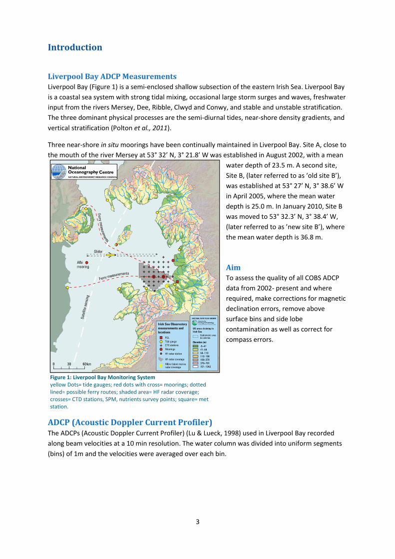
Liverpool Bay (Figure 1) is a semi-enclosed shallow subsection of the eastern Irish Sea. Liverpool Bay

is a coastal sea system with strong tidal mixing, occasional large storm surges and waves, freshwater

input from the rivers Mersey, Dee, Ribble, Clwyd and Conwy, and stable and unstable stratification.

The three dominant physical processes are the semi-diurnal tides, near-shore density gradients, and

vertical stratification (Polton et al., 2011).

Three near-shore in situ moorings have been continually maintained in Liverpool Bay. Site A, close to

the mouth of the river Mersey at 53° 32’ N, 3° 21.8’ W was established in August 2002, with a mean

water depth of 23.5 m. A second site,

Site B, (later referred to as ‘old site B’),

was established at 53° 27’ N, 3° 38.6’ W

in April 2005, where the mean water

depth is 25.0 m. In January 2010, Site B

was moved to 53° 32.3’ N, 3° 38.4’ W,

(later referred to as ’new site B’), where

the mean water depth is 36.8 m.

Aim

To assess the quality of all COBS ADCP

data from 2002- present and where

required, make corrections for magnetic

declination errors, remove above

surface bins and side lobe

contamination as well as correct for

compass errors.

ADCP (Acoustic Doppler Current Profiler) The ADCPs (Acoustic Doppler Current Profiler) (Lu & Lueck, 1998) used in Liverpool Bay recorded

along beam velocities at a 10 min resolution. The water column was divided into uniform segments

(bins) of 1m and the velocities were averaged over each bin.

Figure 1: Liverpool Bay Monitoring System yellow Dots= tide gauges; red dots with cross= moorings; dotted lined= possible ferry routes; shaded area= HF radar coverage; crosses= CTD stations, SPM, nutrients survey points; square= met station.

4

Quality control method A quality control was required to correct the data for magnetic declination errors, remove bins

above the surface and contaminated near surface bins as well as correct for compass errors. Any

changes made to the data during the quality control are noted as comments in the header of each

file and are also remarked in the COBS_ADCP_Data_Catalogue.xls.

1. Corrections

a) Correction for magnetic declination errors Magnetic declination is the angle between magnetic and true north. It varies spatially and with time

due to the change of earth’s magnetic field. Since the previous correction was a fixed value for the

start of the observing period the variation over time was needed.

For each site declinations were calculated using Geomag 7.0 (International Association of

Geomagnetism and Aeronomy, Working Group V-MOD, 2010). The declinations calculated using this

software can be found in the accompanying documentation.

b) Remove bins above the surface The sea surface was calculated using CSIRO seawater toolbox ver.3.2 (Morgans, 2006) from the

pressure. The ADCP pressure record was used for most files, however sometimes this was not

available or faulty then pressure of an alongside ADCP or of a different pressure recording

instrument on the same frame was used. The bins above the surface were blanked with non values

(NaN).

(i) Using backscatter intensity

If no pressure records were available or it could not be used the intensity backscatter was used to

calculate the surface. Backscatter data are collected for each beam thus the average of the four data

sets was used. The sea surface is a relatively hard surface hence it can be detected looking for the

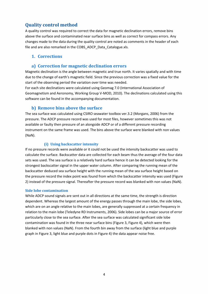
strongest backscatter signal in the upper water column. After comparing the running mean of the

backscatter deduced sea surface height with the running mean of the sea surface height based on

the pressure record the index point was found from which the backscatter intensity was used (Figure

2) instead of the pressure signal. Thereafter the pressure record was blanked with non values (NaN).

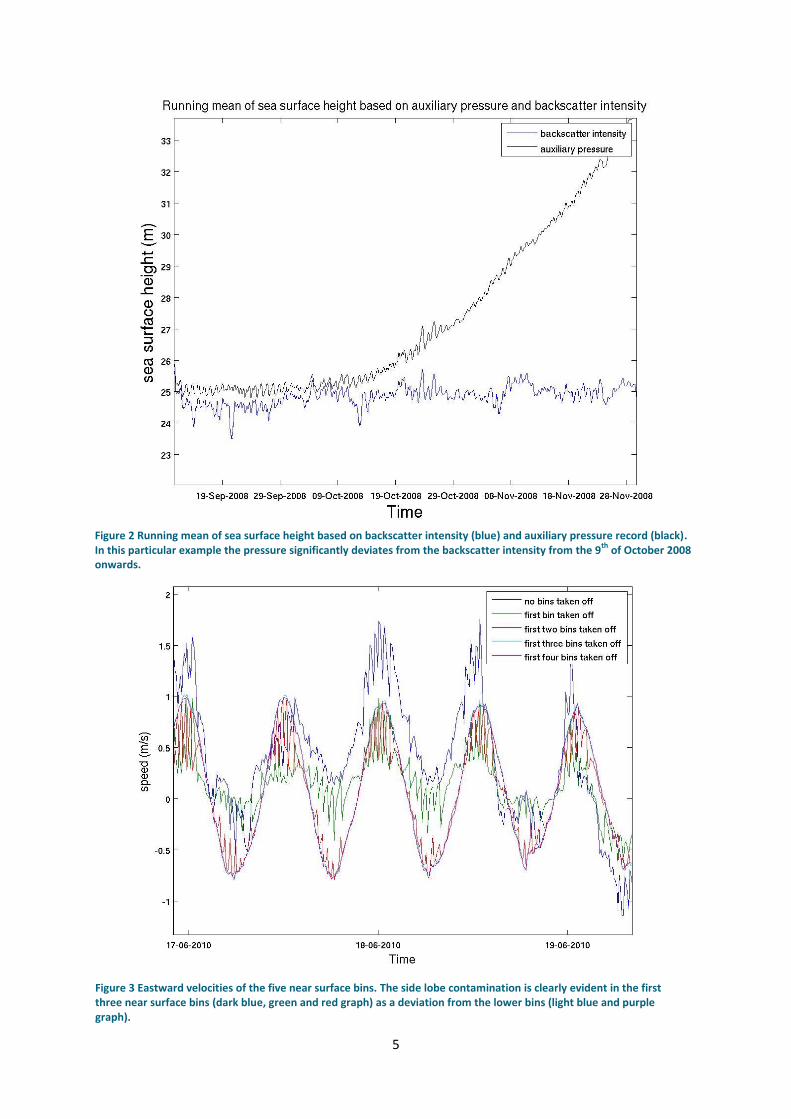
Side lobe contamination

While ADCP sound signals are sent out in all directions at the same time, the strength is direction

dependent. Whereas the largest amount of the energy passes through the main lobe, the side lobes,

which are on an angle relative to the main lobes, are generally suppressed at a certain frequency in

relation to the main lobe (Teledyne RD Instruments, 2006). Side lobes can be a major source of error

particularly close to the sea surface. After the sea surface was calculated significant side lobe

contamination was found in the three near surface bins (Figure 3, Figure 4), which were then

blanked with non values (NaN). From the fourth bin away from the surface (light blue and purple

graph in Figure 3, light blue and purple dots in Figure 4) the data appear noise free.

5

Figure 2 Running mean of sea surface height based on backscatter intensity (blue) and auxiliary pressure record (black). In this particular example the pressure significantly deviates from the backscatter intensity from the 9

th of October 2008

onwards.

Figure 3 Eastward velocities of the five near surface bins. The side lobe contamination is clearly evident in the first three near surface bins (dark blue, green and red graph) as a deviation from the lower bins (light blue and purple graph).

6

c) Correct for compass errors The ADCP is affected by local magnetic fields of batteries, other instruments and the frame it is

mounted on. The data were corrected using measurements that were free of such errors. These data

were available from the HF Radar system (WERA), which observes sea surface currents and waves in

the Liverpool Bay and is also part of the Liverpool Bay Coastal Observatory. Two sites point out on

Liverpool Bay and have a maximum range of nearly 100 km and the resolution for sea surface

currents is 2 km. One site is located at Llanddulas/Abergele, North Wales pointing northwards,

whereas the second site is located at Formby, Merseyside pointing approximately west-south-west.

Sound pulses are sent out and the response is measured every 20 min. Using data from these two

sites enough information is available to calculate sea surface currents and their direction.

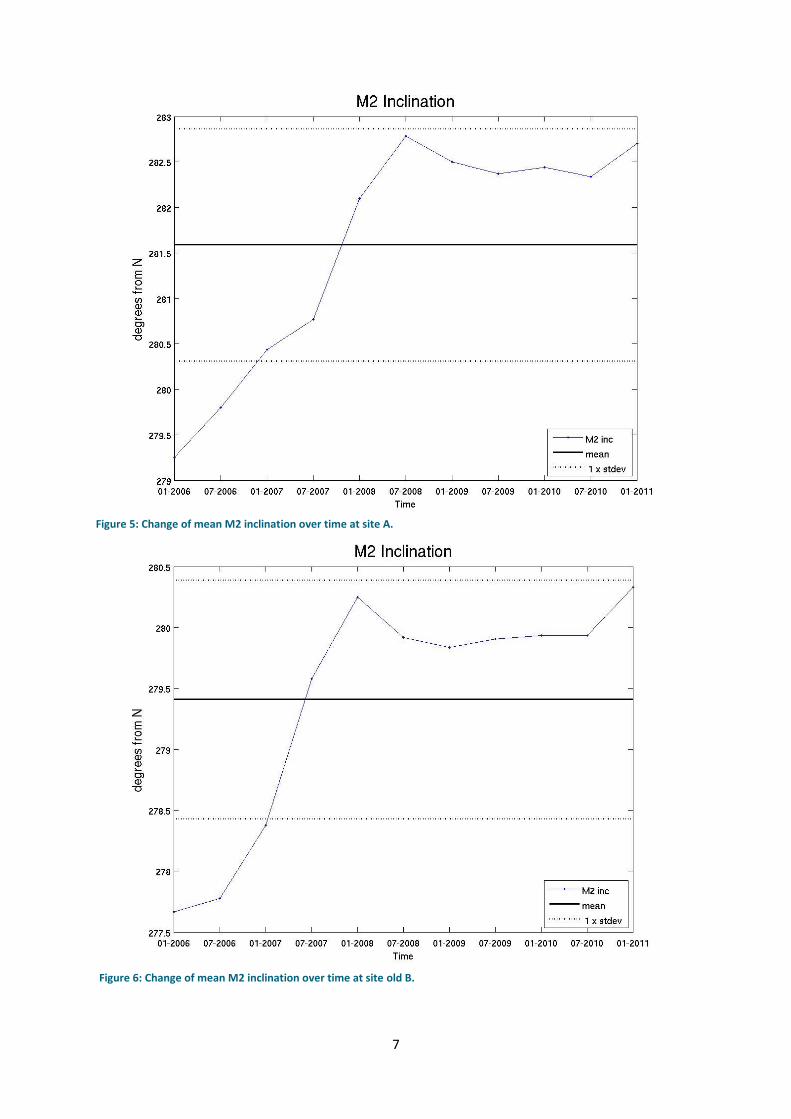
A tidal harmonic analysis (T-tide, Pawlowicz et al., 2002) was used to calculate the ellipse

characteristics of the major tidal current constituent in the radar data. In Liverpool Bay this is the M2

component, which is the principal lunar semi-diurnal tidal constituent. Although the inclination

increases over a period of five years (2006 - 2011) at all three sites this variation is within one

standard deviation (Figure 5, Figure 6, Figure 7), and therefore smaller than the compass accuracy of

2 ° (Teledyne RD Instruments, 2008), which justifies using a mean value as reference for each site.

Figure 4 Current ellipse of near surface bins. First three near surface bins (dark blue, green and red dots) are scattered over the whole profile and show side lobe noise. The current ellipse shows the expected east-west direction only from the fourth bin away from the surface (light blue and purple dots).

7

Figure 5: Change of mean M2 inclination over time at site A.

Figure 6: Change of mean M2 inclination over time at site old B.

8

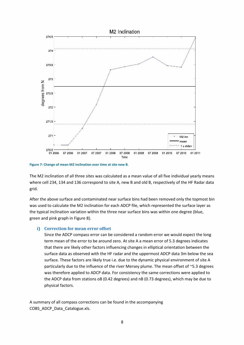
The M2 inclination of all three sites was calculated as a mean value of all five individual yearly means

where cell 234, 134 and 136 correspond to site A, new B and old B, respectively of the HF Radar data

grid.

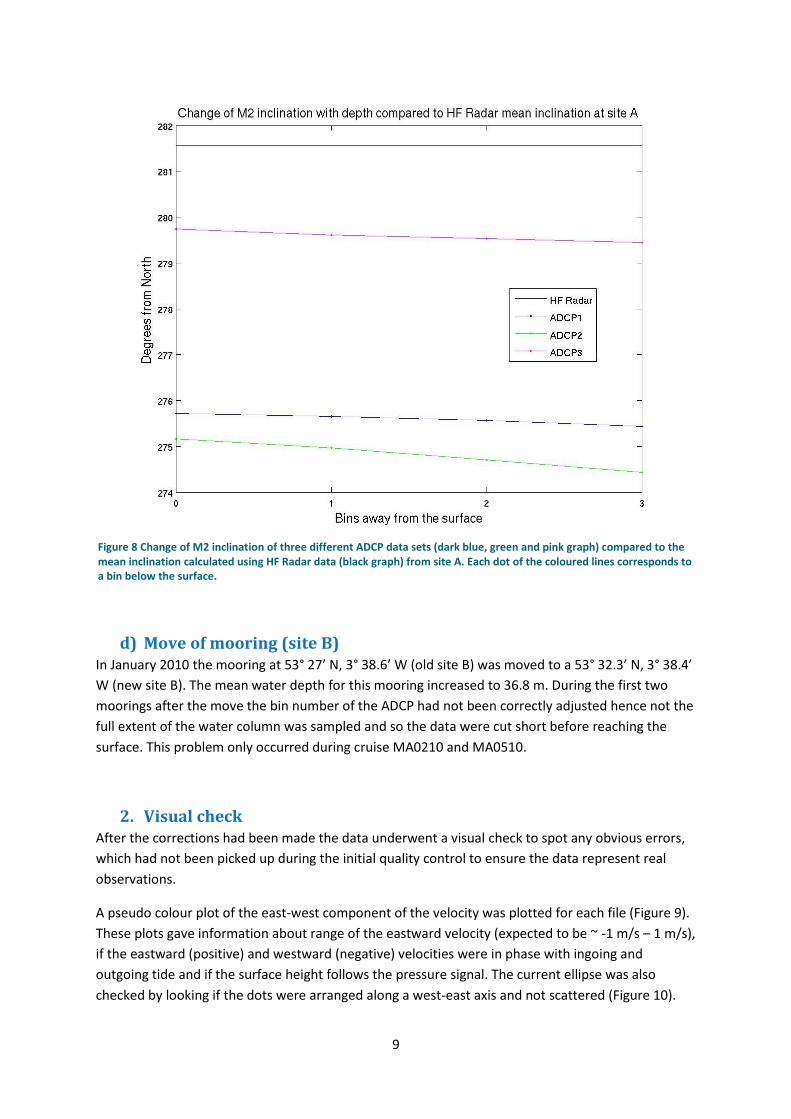
After the above surface and contaminated near surface bins had been removed only the topmost bin

was used to calculate the M2 inclination for each ADCP file, which represented the surface layer as

the typical inclination variation within the three near surface bins was within one degree (blue,

green and pink graph in Figure 8).

i) Correction for mean error offset

Since the ADCP compass error can be considered a random error we would expect the long

term mean of the error to be around zero. At site A a mean error of 5.3 degrees indicates

that there are likely other factors influencing changes in elliptical orientation between the

surface data as observed with the HF radar and the uppermost ADCP data 3m below the sea

surface. These factors are likely true i.e. due to the dynamic physical environment of site A

particularly due to the influence of the river Mersey plume. The mean offset of ~5.3 degrees

was therefore applied to ADCP data. For consistency the same corrections were applied to

the ADCP data from stations oB (0.42 degrees) and nB (0.73 degrees), which may be due to

physical factors.

A summary of all compass corrections can be found in the accompanying

COBS_ADCP_Data_Catalogue.xls.

Figure 7: Change of mean M2 inclination over time at site new B.

9

d) Move of mooring (site B) In January 2010 the mooring at 53° 27’ N, 3° 38.6’ W (old site B) was moved to a 53° 32.3’ N, 3° 38.4’

W (new site B). The mean water depth for this mooring increased to 36.8 m. During the first two

moorings after the move the bin number of the ADCP had not been correctly adjusted hence not the

full extent of the water column was sampled and so the data were cut short before reaching the

surface. This problem only occurred during cruise MA0210 and MA0510.

2. Visual check After the corrections had been made the data underwent a visual check to spot any obvious errors,

which had not been picked up during the initial quality control to ensure the data represent real

observations.

A pseudo colour plot of the east-west component of the velocity was plotted for each file (Figure 9).

These plots gave information about range of the eastward velocity (expected to be ~ -1 m/s – 1 m/s),

if the eastward (positive) and westward (negative) velocities were in phase with ingoing and

outgoing tide and if the surface height follows the pressure signal. The current ellipse was also

checked by looking if the dots were arranged along a west-east axis and not scattered (Figure 10).

Figure 8 Change of M2 inclination of three different ADCP data sets (dark blue, green and pink graph) compared to the mean inclination calculated using HF Radar data (black graph) from site A. Each dot of the coloured lines corresponds to a bin below the surface.

10

Figure 9: Eastward velocity component and pressure record in db.

Figure 10: Current ellipse of the ADCP data. Same coloured dots are data points from the same bin. All dots are arranged along a west-east axis.

11

Cataloguing When a new set of cruise data is available on the Coastal Observatory Website, it is quality

controlled and added to the COBS_ADCP_Data_Catalogue.xls.

The model output of Geomag 7.0 that calculated the declinations can be found in Declinations.doc.

1. COBS ADCP Data Catalogue This document was created to catalogue all recorded and quality controlled ADCP data from 2002 to

present cruises.

The table is designed to show the meta data of ADCP data

collected from 2002 – present.

For each ADCP file, the table shows:

Cruise number and ID

Location of mooring by using the station colour

code (Figure 11).

Applied magnetic declination in N

Applied correction for compass error in N

If the data have been three beam corrected

Figure 11: ADCP Data Catalogue. Header and some quality controlled ADCP data from 2009-2011.

Figure 2: Station colour code.

12

If the auxiliary pressure was used to detect the surface

o And if not what was the source of the replacement pressure or signal to indentify

the surface.

Comments regarding problems that were encountered during the quality control, or why

certain corrections could not be made.

The first sheet is a summary of all processed data from 2002 - present and the following sheets are

yearly summaries.

2. Declinations This document was created to record the full output of Geomag 7.0, which was used to determine

the declinations at site A, old B and new B from 2002 to 2011.

The output of the model shows the model coefficients used, the position in degrees, minutes,

seconds, the altitude, the range of interest and the time steps used. The parameters are:

D: Declination I: Inclination H: Horizontal field strength X: North component Y: East component Z: Vertical component F: Total field strength dD,dI, change per year of

The results are listed for the chosen starting time increasing with the time steps to the end of the

period of interest (Figure 12).The yearly change is also given at the end of the table.

Figure 12: Screenshot of Declinations document.

13

References

International Association of Geomagnetism and Aeronomy, Working Group V-MOD. Participating

members: Finlay, C.C., Maus, S., Beggan, C.D., Bondar, T.N., Chambodut, A., Chernova, T.A.,

Chulliat, A., Golovkov, V.P., Hamilton, B., Hamoudi, M., Holme, R., Hulot, G., Kuang, W Langlais, B.

Lesur, V., Lowes, F.J., Luhr, H., Macmillan, S., Mandea, M., McLean, S., Manoj, C., Menvielle, M.,

Michaelis, I., Olsen, N., Rauberg, J., Rother, M., Sabaka, T.J., Tangborn, A., Toffner-Clausen, L.,

Thebault, E., Thomson, A.W.P., Wardinski, I., Wei, Z., T. I. Zvereva, T.I., (2010). International

Geomagnetic Reference Field: the eleventh generation, Geophys. J. Int., 183, 3, 1216-1230. DOI:

10.1111/j.1365-246X.2010.04804.x.

Lu, Y. and Lueck, R.G. (1999): Using a Broadband ADCP in a Tidal Channel. Part I: Mean Flow and

Shear. Journal of Atmospheric and Oceanic Technology, 16, 1556 – 1567.

Morgan, P. (2006): CSIRO Seawater toolbox ver. 3.2.

Pawlowicz, R., Beardsley, B. and Lentz, S (2002): Classical Tidal Harmonic Analysis Including Error

Estimates in MATLAB using T_TIDE, Computers and Geosciences, 28, 929-937.

Polton J.A., Palmer, M.R. and Howarth, M.J. (2011): Physical and Dynamical Oceanography of

Liverpool Bay. Ocean Dynamics 62, 9, 1421-1439. DOI: 10.1007/s10236-011-0431-6

Teledyne RD Instruments, 2006 : Acoustic Doppler Current Profiler Principles of Operation A Practical Prime

Teledyne RD Instruments, 2008: Workhorse Monitor ADCP Datasheet.